Negative Kaons in Dense Baryonic Matter

Abstract

Kaon polarization operator in dense baryonic matter of arbitrary isotopic composition is calculated including s- and p-wave kaon-baryon interactions. The regular part of the polarization operator is extracted from the realistic kaon-nucleon interaction based on the chiral and $1/N_{c}$ expansion. Contributions of the $\Lambda(1116)$, $\Sigma(1195)$, $\Sigma^{*}(1385)$ resonances are taken explicitly into account in the pole and regular terms with inclusion of mean-field potentials. The baryon-baryon correlations are incorporated and fluctuation contributions are estimated. Results are applied for $K^{-}$ in neutron star matter. Within our model a second-order phase transition to the s-wave $K^{-}$ condensate state occurs at $\rho_{c}\stackrel{{\scriptstyle\scriptstyle>}}{{\phantom{}{}_{\sim}}}4\rho_{0}$ once the baryon-baryon correlations are included. We show that the second-order phase transition to the p-wave $K^{-}$ condensate state may occur at densities $\rho_{c}\sim 3\div 5\rho_{0}$ in dependence on the parameter choice. We demonstrate that a first-order phase transition to a proton-enriched (approximately isospin-symmetric) nucleon matter with a p-wave $K^{-}$ condensate can occur at smaller densities, $\rho\stackrel{{\scriptstyle\scriptstyle<}}{{\phantom{}{}_{\sim}}}2\rho_{0}$. The transition is accompanied by the suppression of hyperon concentrations.

I Introduction

Strangeness modes in compressed hadronic matter stay in the focus of interest over the last decade. Strangeness is considered as a good probe for dynamics of heavy-ion collisions. The vast amount of data is accumulated for different collision energy regimes at GANIL, GSI, CERN and BNL facilities hic . New data are in advent advent . Understanding of strangeness production requires a systematic study of the evolution of virtual strangeness modes in the quark-gluon plasma and in the soup of virtual hadrons. At break-up stage these virtual modes are redistributed between real strange particles which can be observed in experiment.

Other interesting topic is a strangeness content of neutron stars. With density increase strangeness can be liberated and face up in the filling of the hyperon Fermi seas and/or in the creation of kaon condensates. Both mentioned topics need a better knowledge of the kaon-baryon interaction in dense baryonic matter. Question on principal possibility of the kaon condensation in dense nucleon matter was risen in Refs. krive and swave . Occurrence of the kaon condensation in neutron star interiors may have interesting observational consequences: (i) The softening of the equation of state (EoS), due to the appearance of a kaon condensate phase, lowers the maximum neutron star mass and could induce transformation of neutron stars into low-mass black holes bb . (ii) Kaon condensation is predicted to be accompanied with the change of the nucleon isospin composition from the neutron-enriched star ($N>>Z$) to the ’nuclear’ star ($N\sim Z$) or even to the ’proton’ star ($N\stackrel{{\scriptstyle\scriptstyle<}}{{\phantom{}{}_{\sim}}}Z$), where the electric charge of protons is compensated by the charge of the condensed kaons kvk95 . (iii) The enhanced neutrino-emission processes, occurring on protons in the proton-enriched matter and on the kaon condensate field, lead to substantially more rapid cooling of the star nscool .

The $K^{-}$ condensate is created in neutron stars due to weak multi-particle processes

$$e^{-}+X\to K^{-}+X^{\prime}\,,\qquad n+X\to p+K^{-}+X^{\prime},$$ (1)

in which electrons are replaced by $K^{-}$ mesons, and neutrons are converted into protons and $K^{-}$ swave-1 . The symbolic writing (1) assumes that surrounding baryons ($X,X^{\prime}$) assure the momentum conservation, therefore the critical point is determined by the energy balance only. These processes become possible, if the electron chemical potential $\mu_{e}$ exceeds the minimal $K^{-}$ energy,

$$\omega^{\rm min}(\boldsymbol{k}_{m})=\min_{\boldsymbol{k}}\{\omega^{\rm min}(\boldsymbol{k})\}\,,$$

where $\omega^{\rm min}(|\boldsymbol{k}|)$ is the $K^{-}$ energy at the lowest (index ”$\rm min$”) quasiparticle spectrum branch of $K^{-}$ excitations in neutron star matter. The works swave ; swave-1 ; swave-2 and subsequent ones have postulated that there is only one kaon branch, for which $\omega(\boldsymbol{k}=0)\rightarrow m_{K}$ ($m_{K}$ is the kaon mass) for the baryon density $\rho\rightarrow 0$, and the minimum is achieved at $\boldsymbol{k}_{m}=0$. Then the critical point of the s-wave $K^{-}$ condensation in a second-order phase transition is determined by the condition $\omega(\boldsymbol{k}=0)=\mu_{e}$. The first-order phase transition to the kaon condensate state was investigated in Ref. tpl94 applying the Maxwell construction principle and in Ref. gs according to Gibbs criteria. The p-wave kaon-nucleon interaction, which changes the momentum dependence of the kaon spectrum, was disregarded in those works. The p-wave $\Lambda(1116)$-nucleon hole and $\Sigma(1195)$-nucleon hole contributions to the kaon polarization operator were introduced in Ref. pw in the framework of the chiral SU(3) symmetry. However then authors focused on the discussion of the s-wave kaon condensation and considered the polarization operator at zero momentum.

Ref. kvk95 worked out a possibility of the p-wave kaon condensation. The kaon polarization operator was constructed with inclusion of the $\Lambda(1116)$–nucleon-hole and $\Sigma(1195)$–nucleon-hole contributions in the p-wave part of the kaon polarization operator and the kaon-pion and kaon-kaon interactions. The multi-branch spectrum of $K^{-}$ mesons was found and the possibility of the p-wave kaon condensation related to the population of hyperon–nucleon-hole modes was demonstrated. Possibilities of first-order phase transitions in neutron star interiors to a proton-enriched matter with a p-wave $K^{-}$ condensate and to a neutron-enriched matter with a p-wave $\bar{K}^{0}$ condensate were suggested.

Ref. muto considered the case of a large hyperon admixture in the neutron star core. In such a medium both $K^{-}$ and $K^{+}$ spectra possess extra branches associated with the particle-hole excitations $\Xi-\Lambda^{-1}$, $\Xi-\Sigma^{-1}$ for $K^{-}$ and $N-\Lambda^{-1}$, $N-\Lambda^{-1}$ for $K^{+}$ (hole states are labeled here by tense (-1)). At quite large kaon momenta the branches of $K^{+}$ and $K^{-}$ spectra merge, that signals an instability with respect to $K^{+}K^{-}$ pair creation.

The analyses kvk95 ; muto relied heavily on the pole approximation for the particle-hole diagrams. The final width effects were thereby disregarded too. Question on the presence or absence of the quasiparticle branches in the $K^{-}$ spectrum depends on the kaon energy and on the strength of the s- and p-wave attraction kv99 . The short-range baryon-baryon correlations, which, as a rule, suppress attraction, were disregarded in kvk95 ; muto for simplification. A particular role of the correlations for the p-wave has been taken over in Ref. kv98 . However, the relative strength of s- and p-wave attraction remained model dependent because no systematic investigation of the kaon-nucleon interaction including s- and p-waves has been available that time.

Recently, the $K^{-}$-nucleon scattering has been studied in the framework of the relativistic chiral SU(3) Lagrangian imposing constraints from the $K^{+}$-nucleon and pion-nucleon sectors lk01 . The covariant coupled-channel Bethe-Salpeter equation was solved with the interaction kernel truncated to the third chiral order including the terms which are leading in the large $N_{c}$ limit of QCD. All SU(3) symmetry-breaking effects are well under control by combined chiral and large $N_{c}$ expansions. This analysis gives an opportunity to extend results of  kvk95 ; kv98 taking into account off-pole (regular background) contributions to the kaon self-energy. The accurate fit of experimental data achieved in Ref. lk01 fixes the values of the kaon-nucleon-hyperon coupling constants. Particularly, the $\Sigma^{*}(1385)$-pole contribution to the kaon-nucleon scattering was proved to be sizable, being not included in works Ref. kvk95 ; muto .

The discussion of the s-wave and, especially, of the p-wave kaon-baryon interactions in nuclear matter is important for the kaon production in heavy ion collisions kvk96 . The momentum dependence of kaon yields is experimentally measured kaos . Also, the multi-branch $K^{-}$ spectrum can be tested via $\bar{\nu}$-scattering on atomic nuclei kv98 . Peculiarities of the $K^{-}$-nucleon interaction near mass shell are of great importance for the physics of $K^{-}$ atoms LF01 ; Oset .

In this work we continue the study of the s- and p-wave $K^{-}$-baryon interactions in dense baryonic matter of arbitrary isotopic composition. In particular, we present our results for the composition typical for the core of neutron stars. Our strategy to verify possibilities of s- and p-wave condensations is as follows. For given total baryon density and the composition of the neutron star matter we find the $K^{-}$ energy at lowest branch of the dispersion equation as a function of the momentum and then find the minimum in respect to momenta. At density, when $\omega^{\rm min}(\boldsymbol{k}_{m})$ meets the electron chemical potential $\mu_{e}$, the reactions (1) become to be possible and the system undergos a second-order phase transition developing a classical field with the $K^{-}$ quantum numbers. If this state is realized for $\boldsymbol{k}_{m}=0$, we deal with the s-wave kaon condensation and, if $\boldsymbol{k}_{m}\neq 0$, we deal with the p-wave condensation.

Since solutions depend on many rather uncertain parameters, we study possibilities of s- and p-wave condensations separately. For instance, discussing possibility of the s-wave condensation we put $\boldsymbol{k}=0$ in the solution $\omega^{\rm min}(\boldsymbol{k})$, assuming that parameters of the p-wave interaction are such that they do not allow for the p-wave condensation at the critical density for the s-wave condensation. Then, trying to find a most appropriate parameter choice we investigate how the possibility of the s-wave condensation depends on a parameter variation. Next, in the same manner we study a possibility of the p-wave condensation. Then we find the energy and pressure of the system with the kaon condensate at different spin-isospin compositions and densities. The system selects the spin-isospin composition corresponding to the minimum of the energy. We compare the pressure of the system with the kaon condensate with the pressure of the neutron star matter without condensate. If at some density the pressure and the nucleon chemical potential of the system with the kaon condensate coincide with those values of the neutron star matter (other density and isospin composition) without the condensate the system may come to the condensate state by the first order phase transition. Such a transition starts at a density described by the Maxwell construction. It occurs if an effective surface tension parameter is rather large. Otherwise, if an effective surface tension parameter is not too large, a mixed phase is realized starting from even smaller densities.

In this paper we describe the baryon matter in terms of the relativistic mean-field model (Sec. II). In Sec. III we introduce the kaon-nucleon interaction in vacuum, as it follows from the partial wave analysis of Ref. lk01 . Then we separate the pole contributions of $\Lambda(1116)$, $\Sigma(1195)$ and $\Sigma^{*}(1385)$ hyperons in p-waves. Sections IV through VII are devoted to the construction of the kaon polarization operator. We start in Sec. IV with the polarization operator in the gas approximation but including the mean-field potentials acting on baryons. Besides the $\Lambda(1116)$, $\Sigma(1195)$ and $\Sigma^{*}(1385)$-nucleon-hole contributions it contents a regular attractive part, weakly dependent on the kaon energy. In Sec. V we separate s- and p-wave parts of the kaon polarization operator. Occupation of hyperon Fermi seas is incorporated in Sec. VI. Repulsive baryon-baryon correlations are evaluated and included in the hyperon-nucleon particle-hole channels and in the regular part of the polarization operator in Sec. VII. In each section above we illustrate the strength of new terms included into the polarization operator and suggest effective parameterizations. We relegate the discussion of contributions from kaon fluctuations (baryon self-energies, multi-loop corrections) to Appendix D. We argue that these effects do not modify substantially the kaon polarization operator at zero temperature in the region of small kaon energies and momenta, which is of our interest here. In Sect. VIII we analyze different possibilities of second- and first-order phase transitions to the s- and p-wave $K^{-}$ condensate states. In particular, we argue for the p-wave $K^{-}$ condensation at $\rho\stackrel{{\scriptstyle\scriptstyle<}}{{\phantom{}{}_{\sim}}}2\rho_{0}$ ($\rho_{0}\simeq 0.17$ fm^-3 is density of nuclear saturation) arising via a first-order phase transition. In this phase transition all the hyperon Fermi seas are melted and neutron star matter becomes proton-enriched (with approximately symmetric isospin composition, $N\simeq Z$). Dependence of the results on the specifics of the EoS and the corresponding particle composition is illustrated in Appendix  A. Some technical information on the Green’s functions and the Lindhard’s function is deferred to Appendices  B and C.

Throughout the paper we use units $\hbar=c=1$.

II Baryon Interaction in Relativistic Mean Field Model

II.1 Lagrangian of the Model

We consider a dense system consisting of baryons and leptons, which we describe by the Lagrangian density containing the baryon and the lepton contributions, respectively: ${\cal L}={\cal L}_{B}+{\cal L}_{l}$ .

The baryon matter at densities relevant for neutron star interiors is convenient to describe by the mean-field solution of the Lagrangian walecka :

$${\cal L}_{B}=\sum_{B}\!\bar{B}\!\left(i\,\partial\!\!\!/-g_{\omega B}\omega\!\!\!/-g_{\rho B}\,\boldsymbol{\rho}\!\!\!/\cdot\boldsymbol{t}_{B}-m_{B}+g_{\sigma B}\sigma\right)\!B$$

$$+\frac{\partial_{\mu}\sigma\partial^{\mu}\sigma}{2}-\frac{m_{\sigma}^{2}\sigma^{2}}{2}-\frac{m_{N}b(g_{\sigma N}\sigma)^{3}}{3}-\frac{c(g_{\sigma N}\sigma)^{3}}{4}$$

$$-\frac{\omega_{\mu\nu}\,\omega^{\mu\nu}}{4}+\frac{m_{\omega}^{2}\omega_{\mu}\,\omega^{\mu}}{2}-\frac{\rho_{\mu\nu}\,\rho^{\mu\nu}}{4}+\frac{m_{\rho}^{2}\boldsymbol{\rho}_{\mu}\boldsymbol{\rho\,}^{\mu}}{2},$$ (2)

where all states of the baryon ($J^{P}=\frac{1}{2}^{+}$) octet $B=(n,p,\Lambda\,,\Sigma^{\pm,0}\,,\Xi^{-0})$, interact via exchange of scalar, vector and isovector mesons $\sigma$ , $\omega_{\mu}$ , $\boldsymbol{\rho}_{\mu}$. Heavier baryons do not appear at the baryon densities under consideration ($\rho\leq 6\rho_{0}$) and are not included, therefore. In (2) $\boldsymbol{t}_{B}$ denotes isospin operator acting on the baryon $B$. The field strength tensors for the vector mesons are given by $\omega_{\mu\nu}=\partial_{\mu}\,\omega_{\nu}-\partial_{\nu}\,\omega_{\mu}$ for omega mesons and $\rho_{\mu\nu}=\partial_{\mu}\,\boldsymbol{\rho}_{\nu}-\partial_{\nu}\,\boldsymbol{\rho}_{\mu}$  for rho mesons. The equations of motion for baryons following from (2) give

$$E_{B}(\boldsymbol{p})=\epsilon_{B}(\boldsymbol{p})+V_{B}\,,\qquad\epsilon_{B}(\boldsymbol{p})=\sqrt{m_{B}^{*2}+\boldsymbol{p}^{2}}\,,$$ (3)

where $m_{B}^{*}=(m_{B}-g_{\sigma B}\,\sigma)$ is the baryon effective mass, and $V_{B}=g_{\omega\,B}\,\omega_{0}+g_{\rho\,B}\,\rho_{03}\,t_{3\,B},$ with $\sigma,\omega_{0},\rho_{03}$ being the mean field solutions of equations of motion for the meson fields. The composition of the cold neutron star matter at baryon density $\rho$ is determined by the $\beta$-equilibrium conditions $E_{B}(p_{{\rm F}B})=\mu_{n}-q_{B}\,\mu_{e}$. Here $p_{{\rm F}B}$ is the Fermi momentum, $q_{B}$ is the electric charge of the given baryon species $B$, and $\mu_{n}$ , $\mu_{e}$ are chemical potentials of neutrons and electrons fixed by the total baryon density $\rho$ and the electroneutrality condition.

The lepton Lagrangian density is the sum of the free electron and $\mu^{-}$ meson contributions ${\cal L}_{l}={\cal L}_{e}+{\cal L}_{\mu}$ . The $\beta$-equilibrium requires that the muon chemical potential equals to the electron one, $\mu_{\mu}=\mu_{e}$, and, therefore, muons appear in the system when $\mu_{e}$ exceeds the muon mass, $m_{\mu}$ . Electrons can be considered as ultra-relativistic particles.

The energy density of the system is given by

$$E_{\rm tot} = E_{\rm mes}+\sum_{B}E_{B}^{\rm kin}(p_{{\rm F}B})+\sum_{l=e^{-},\mu^{-}}E_{l}(\mu_{e}),$$

$$E_{\rm mes} = \frac{1}{3}\,b\,m_{N}\,(g_{\sigma\,N}\,\sigma)^{3}+\frac{1}{4}\,c\,(g_{\sigma\,N}\,\sigma)^{4}$$

$$+ \frac{1}{2}\,m_{\sigma}^{2}\,\sigma^{2}+\frac{1}{2}\,m_{\omega}^{2}\,\omega_{0}^{2}+\frac{1}{2}\,m_{\rho}^{2}\,\rho_{03}^{2},$$

$$E_{B}^{\rm kin}(p_{{\rm F}B}) = \frac{1}{\pi^{2}}\,\intop_{0}^{p_{{\rm F}B}}\,dp\,p^{2}\,\epsilon_{B}(p)\,,\quad$$

$$E_{\rm lept}(\mu_{l}) = \frac{1}{\pi^{2}}\,\theta(\mu_{l}-m_{l})\intop_{m_{l}}^{\mu_{l}}\,d\epsilon\,\epsilon^{2}\,\sqrt{\epsilon^{2}-m_{l}^{2}},$$ (4)

where $\theta(x)$ is the step function.

II.2 Coupling Constants

The coupling constants are adjusted to reproduce properties of equilibrium nuclear matter: saturation density $\rho_{0}$, binding energy $E_{\rm bind}$, compressibility modulus $K$, and the effective nucleon mass $m_{N}^{*}(\rho_{0})$. In the following we take the value $\rho_{0}=0.17$ fm^-3, and the binding energy $E_{\rm bind}=-16$ MeV. For the nuclear compressibility modulus we take the value $K=$210 MeV, which follows from the variational calculation softeos . Following Ref. walecka we adopt the symmetry energy $a_{\rm sym}=36.8$ MeV which lies well in the interval allowed by the microscopic calculations Lombardo . We take the effective nucleon mass $m_{N}^{*}(\rho_{0})=0.85\,m_{N}$, cf. argumentation in Ref. MSTV90 . Of course, the values of the input parameters can be selected differently, in order to fit experimental data. We refer at this point to the recent work Piek discussing the uncertainties.

The corresponding coupling constants of the Lagrangian (2) are:

$$\frac{\displaystyle g_{\omega N}^{2}\,m_{N}^{2}}{\displaystyle m_{\omega}^{2}}=54.6041\,,\quad\frac{\displaystyle g_{\sigma N}^{2}\,m_{N}^{2}}{\displaystyle m_{\sigma}^{2}}=164.462\,,$$

$$\frac{\displaystyle g_{\rho N}^{2}\,m_{N}^{2}}{\displaystyle m_{\rho}^{2}}=121.690\,,\quad b=0.0202832\,,$$

$$c=0.0471633\,.$$

In order to verify the sensitivity of the results to the details of the EoS we explore in Appendix A another set of the nuclear matter parameters, which we fit to reproduce the microscopic calculations of Urbana-Argonne group Akmal .

Including hyperons, one also has to specify hyperon couplings to the meson fields. They are expressed via ratios to the nucleon couplings, $x_{MH}=g_{MH}/g_{MN}$ with $M=(\sigma,\omega,\rho)$ and $H=(\Lambda,\Sigma,\Xi)$. Couplings to the vector mesons are estimated from the quark counting as $x_{\omega\Lambda(\Sigma)}=x_{\rho\Sigma}=\frac{2}{3}$ and $x_{\omega\Xi}=x_{\rho\Xi}=\frac{1}{3}$. Alternatively, relying on SU(3) symmetry sbg one would find $x_{\rho\Sigma}=x_{\rho\Xi}=1$ for the $\rho$ meson couplings. The scalar meson couplings can be constrained by making use of hyperon binding energies in infinite nuclear matter at saturation glenmos , extrapolated from hyper-nucleus data. Denoting the binding energy of a hyperon by $E_{\rm bind}^{H}$ we derive the following relation between the scalar and vector couplings:

$$E_{\rm bind}^{H} = (g_{\omega N}^{2}\,\rho_{0}/m_{\omega}^{2})\,x_{\omega H}-(m_{N}-m_{N}^{*})\,x_{\sigma H}$$

$$= (80.73\,x_{\omega H}-140.70\,x_{\sigma H})~{}{\rm MeV}.$$

There is convincing evidence from the systematic study of hypernuclei that for $\Lambda$ particles $E_{\rm bind}^{\Lambda}\simeq-30$ MeV lnucl . For $\Sigma$ hyperons in nuclei, on the other hand, the data are still controversial, giving the broad band, $-10~{}{\rm MeV}<E_{\rm bind}^{\Sigma}<30~{}{\rm MeV}$ , from a slight attraction to a strong repulsion sbind . Following Ref. xibind we adopt for $\Xi$ the values $E_{\rm bind}^{\Xi}\simeq-18$ MeV advocated in Ref. sbg .

To cover different possibilities we consider four cases: (I) vector meson couplings are taken according to the quark counting, $x_{\omega\Lambda(\Sigma)}=x_{\rho\Sigma}=2\,x_{\omega\Xi}=2\,x_{\rho\Xi}=\frac{2}{3}$ and $E_{\rm bind}^{\Lambda}=-30$ MeV, $E_{\rm bind}^{\Xi}=-18$ MeV, $E_{\rm bind}^{\Sigma}=30$ MeV; (II) the same as in case (I) but $E_{\rm bind}^{\Sigma}=-10$ MeV; (III) the same as in case (I) but the rho meson couplings are taken according to SU(3) symmetry, i.e. $x_{\rho\Sigma,\Xi}=1$; (IV) the same as in case (III), but for $E_{\rm bind}^{\Sigma}=-10$ MeV.

II.3 Particle Concentrations

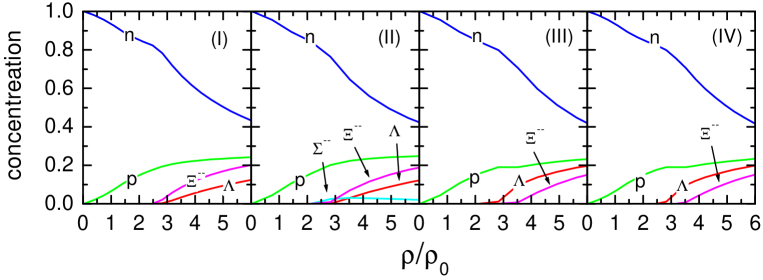
Figure 1: Concentration of baryon species in neutron star matter. Panels (I-IV) correspond to four choices of the hyperon-nucleon interaction constants specified in text.

In Fig. 1 we show the resulting concentrations of different baryon species, as function of the baryon density. Columns (I-IV) correspond to the four above choices of the hyperon-meson coupling constants. We see, that hyperons appear in neutron star matter in all cases at density $\rho>\rho_{{\rm c},H}\simeq 2.5\div 3\,\rho_{0}$. The latter critical value is rather insensitive to various choices of hyperon-nucleon interactions. However, the order, in which hyperons populate the Fermi seas, depends crucially on the details of hyperon-nucleon interactions. The $\Sigma^{-}$ hyperons do not appear, at least, up to $6\rho_{0}$ except for case II. However, even in this case their concentration is very small. The place of $\Sigma^{-}$ is readily taken by $\Xi^{-}$ and $\Lambda$ hyperons. This observation is in line with the results of work gcoupl . In case IV, we chose $E_{\rm bind}^{\Sigma}<0$, nevertheless the $\Sigma$ hyperons do not appear due to increasing repulsion mediated by $\rho$ meson with larger coupling constants than in case II. We see that in all cases I - IV the proton concentration and the electron chemical potential saturate with the filling of hyperon Fermi seas, in line with the results of previous works. We also see that all choices I - IV do not support effects observed in muto , where $\Lambda$ hyperons become more abundant than protons already at $3\rho_{0}$. Therefore, the p-wave $K^{+}K^{-}$ condensation discussed in muto does not show up in the framework of our model for all four parameter choices.

Although concentration of hyperons is rather small in all the cases, their presence may have significant consequences affecting critical densities of p-wave $K^{-}$ condensates.

III $K^{-}$-Nucleon Interaction in Vacuum

The kaon-nucleon interaction in vacuum results as the solution of the coupled-channel Bethe-Salpeter equation

$$\parbox{213.39566pt}{ \includegraphics[clip={true},width=213.39566pt]{t.eps}}\,,$$ (5)

where the triangle is the full meson-baryon scattering amplitude with strangeness (-1) and the circle stands for the interaction kernel. This equation involves rescatterings through all possible meson-baryon intermediate states allowed by the strangeness conservation. The interaction kernel can be derived from SU(3) chiral Lagrangians kaiser ; krippa ; or98 ; om01 or phenomenologically adjusted to fit the data within the K-matrix formalism kmatrix ; keil .

In view of the general interest to the s-wave kaon condensation prevailing in the literature so far, the most attention has been paid to the kaon-nucleon interaction in the s-wave. Although far below the threshold the s-wave kaon-nucleon scattering amplitude is rather smooth function of the kaon energy, close to the threshold the amplitudes vary strongly due to the $\Lambda(1405)$ resonance (see Fig. 2). Therefore, extrapolation of the scattering amplitude, adjusted to fit the data above the $K^{-}N$ threshold, into the subthreshold region crucially depends on the microscopic model applied. Its in-medium modification is a matter of debate, too smed ; RO00 ; ske ; tolos ; KL01 .

Up to recent, only a scarce information on the p-wave kaon-nucleon interaction was available. In the isospin-zero channel the small p-wave amplitudes were not separated from the large contribution of the $\Lambda(1405)$ resonance in the s-wave, which dominates near threshold energies. In the isospin-one channel determination of the p-wave amplitudes remained also uncertain due to a lack of direct experimental information on the $K^{-}n$ scattering at low energies. This gap has been filled by Ref. lk01 , where the relativistic chiral SU(3) Lagrangian imposed extra constrains from the $K^{+}$-nucleon and pion-nucleon sector. This analysis provides reliable estimates for both the s- and p-wave $K^{-}N$ scattering amplitudes, which we will use in the following.

III.1 Forward Scattering Amplitudes

The vacuum $\overline{K}N$ forward scattering amplitudes in the given isospin channel $I$ have contributions from s- and p-partial waves:

$$T^{\rm(I)}(s)=T_{\rm S}^{\rm(I)}(s)+T_{\rm P}^{\rm(I)}(s) = \frac{\bar{E}(s,m_{N}^{2},m_{K}^{2})+m_{N}}{2\,m_{N}}\,\left[F_{\rm S}^{\rm(I)}(s)+Q^{2}(s,m_{N}^{2},m_{K}^{2})\,F_{\rm P}^{\rm(I)}(s)\right]\,,$$

$$Q^{2}(s,p^{2},k^{2}) = \frac{(s-p^{2}-k^{2})^{2}-4\,k^{2}\,p^{2}}{4\,s}\,,$$ (6)

where $s=(p+k)^{2}$, and $p=(\epsilon_{N}(\boldsymbol{p\,}),\boldsymbol{p}\,)$, $k=(\omega,\boldsymbol{k\,})$ are 4-momenta of the incoming nucleon and kaon, respectively. For nucleons and kaons being on mass-shell, the quantity $Q^{2}(s,m_{N}^{2},m_{K}^{2})$ is nothing else but the square of the center-of-mass momentum in the kaon-nucleon channel, $\bar{E}(s,m_{N}^{2},m_{K}^{2})=\sqrt{m_{N}^{2}+Q^{2}(s,m_{N}^{2},m_{K}^{2})}$ is the nucleon energy in the center-of-mass frame,

$$\bar{E}(s,p^{2},k^{2})=\frac{s+p^{2}-k^{2}}{2\sqrt{s}}\,,$$

$m_{N}$ and $m_{K}$ are the free nucleon and kaon masses. We shall neglect the isospin symmetry breaking within kaon and nucleon isospin multiplets, which are irrelevant in dense nuclear matter.

The invariant partial-wave amplitudes $F_{\rm S}^{\rm(I)}$ and $F_{\rm P}^{\rm(I)}$ are related to the standard partial wave amplitudes (cf. Landoldt , section 3.1 for definitions) as

$$F_{\rm S}^{\rm(I)}(s) = \frac{8\,\pi\sqrt{s}}{m_{N}+\bar{E}(s,m_{N}^{2},m_{K}^{2})}\,f_{0+}^{\rm(I)}(s),$$

$$F_{\rm P}^{\rm(I)}(s) = \frac{8\,\pi\sqrt{s}/Q^{2}(s,m_{N}^{2},m_{K}^{2})}{m_{N}+\bar{E}(s,m_{N}^{2},m_{K}^{2})}$$ (7)

$$\times\left(f_{1-}^{\rm(I)}(s)+2\,f_{1+}^{\rm(I)}(s)\right)\,.$$

The partial amplitudes $f_{l\pm}=f_{l,\,J=l\pm\frac{1}{2}}$ in (7) are the scattering amplitudes for the given angular momentum $l$ and total momentum $J$. Real parts of the partial amplitudes $T_{\rm S}^{\rm(I)}$ and $T_{\rm P}^{\rm(I)}$ are shown in Fig. 2 and Fig. 3 by solid lines. Pronounced peak structures in the p-wave amplitude are due to the $\Lambda(1116)$ pole in the isospin-zero channel and the $\Sigma(1195)$ and $\Sigma^{*}(1385)$ poles in the isospin-one channel.

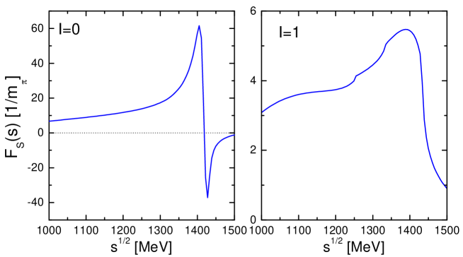
Figure 2: Real parts of the s-wave kaon-nucleon scattering amplitudes in isospin-zero and isospin-one channels lk01 .

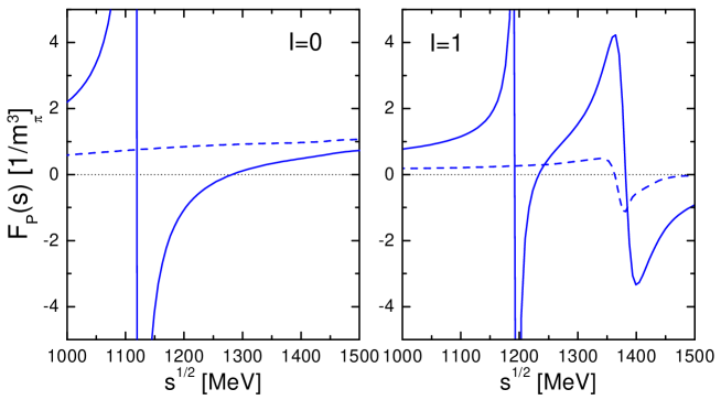
Figure 3: Real parts of the p-wave kaon-nucleon scattering amplitudes $F_{\rm P}$ in isospin zero and isospin one channels (solid lines) lk01 . The dash lines represent corresponding pole subtracted scattering amplitudes (8).

III.2 Separation of the Pole Terms

The hyperon s-channel exchanges are responsible for the most strong variation of the polarization operator at low frequencies and momenta. Therefore, they deserve a special consideration in view of the baryon modifications by the mean field-potentials. To treat them explicitly, we separate pole contribution from the p-wave amplitudes. Then we define the pole and pole-subtracted amplitudes

$$\delta F_{\rm P}^{({\rm I})}(s) = F_{\rm P}^{({\rm I})}-F_{\rm pole}^{({\rm I})}(s)\,,$$ (8)

$$F_{\rm pole}^{(0)}(s) = -2\,\frac{C_{KN\Lambda}^{2}\,2\,m_{\Lambda}\,}{(\bar{E}(s,p^{2},k^{2})+m_{N})^{2}}\frac{(m_{\Lambda}+m_{N})^{2}}{s-m_{\Lambda}^{2}+i\,0},$$ (9)

$$F_{\rm pole}^{(1)}(s) = -2\,\frac{C_{KN\Sigma}^{2}\,2\,m_{\Sigma}\,}{(\bar{E}(s,m_{N}^{2},m_{K}^{2})+m_{N})^{2}}\,\frac{(m_{\Sigma}+m_{N})^{2}}{s-m_{\Sigma}^{2}+i\,0}$$ (10)

$$-\frac{4}{3}\,\frac{2\,C_{KN\Sigma^{*}}^{2}\,(s/m_{\Sigma^{*}})}{s-m_{\Sigma^{*}}^{2}+\frac{i}{2}\,\gamma_{\Sigma^{*}}(s)}\,\frac{\bar{E}(m_{\Sigma^{*}}^{2},m^{2}_{N},m^{2}_{K})+m_{N}}{\bar{E}(s,m_{N}^{2},m_{K}^{2})+m_{N}}\,.$$

The $\Sigma^{*}$ width, $\gamma_{\Sigma^{*}}(s)=(\sqrt{s}+m_{\Sigma^{*}})\,(\gamma_{\pi\Lambda}(s)+\gamma_{\pi\Sigma}(s)+\gamma_{KN}(s))$, includes contributions of $\pi\Lambda$ , $\pi\Sigma$ and $KN$ channels, $\gamma_{\phi B}(s)=C_{\phi B\Sigma^{*}}^{2}\,(m_{B}+\bar{E}(s,m_{B}^{2},m_{\phi}^{2}))|Q(s,m_{B}^{2},m_{G}^{2})|^{3}/(12\,\pi\,\sqrt{s})\,$, where $m_{B}$ is the mass of the corresponding baryon $B=(n,p,\Lambda\,,\Sigma^{\pm,0}\,,\Xi^{-0})$ and $m_{\phi}$ is the mass of the corresponding light meson $\phi=(\boldsymbol{\pi},\boldsymbol{K})$. The coupling constants $C_{\pi\Lambda(\Sigma)\Sigma^{*}}$ can be extracted from the partial width of the $\Sigma^{*}$ hyperon. The values of the $KN\Lambda(\Sigma)$ coupling constants $C_{KN\Lambda}\simeq-0.68/m_{\pi}$, $C_{KN\Sigma}\simeq 0.34/m_{\pi}$ entering (9,10) follow directly from the amplitudes shown in Fig. 3. The values of $C_{KN\Lambda}$ and $C_{KN\Sigma}$ are defined as couplings of $\Lambda$ to $(K^{\dagger}N)$ and $\Sigma^{\alpha}$ to $(K^{\dagger}\tau^{\alpha}N)$ isospin states, where $K$, $N$ stand for isospin-doublets, $\Sigma^{\alpha}$ is the isospin-triplet, and $\tau^{\alpha}$ are the isospin Pauli matrices. Note that the value of $C_{KN\Lambda}$, obtained on basis of Ref. lk01 , is smaller than that fitted by Jülich group Julich and then used in Refs. pw ; kvk95 .

The scattering amplitude nearby the $\Sigma^{*}$ resonance can be only approximately described by the last term in (10), since the corresponding amplitude results from a multi-channel dynamics, which generates the energy dependent self-energy of the $\Sigma^{*}$ resonance to be included in the denominator. This self-energy, however, can be neglected at $\sqrt{s}$ relevant for calculations below. Ref. lk01 gives the value for the $\Sigma^{*}$ resonance coupling $C_{KN\Sigma^{*}}\simeq 0.84/m_{\pi}$ defined by the Lagrangian term $C_{KN\Sigma^{*}}\bar{\Sigma}^{*\alpha}_{\mu}\partial^{\mu}K^{\dagger}\tau^{\alpha}N$ .

The pole subtracted amplitudes $\delta F^{\rm(I)}(s)$ are shown in Fig. 3 by dash lines. We see that the amplitudes in both isospin channels are smooth functions of $\sqrt{s}$ in the subthreshold region $\sqrt{s}<1300$ MeV of interest.

Nevertheless, we would like to notice that procedure of the pole subtraction is not unambiguous. The forms (9,10), chosen here, will later exhibit themselves to be convenient, since they allow direct comparison with the analysis of Ref. kvk95 ; kv99 ; muto .

Considering further the kaon-nucleon interaction in dense matter, we also need to take into account the mean-field potentials acting on baryons according to the Lagrangian (2).

IV $K^{-}$ Polarization Operator from Scattering Amplitudes

IV.1 Gas Approximation and Baryonic Mean-Fields

Our further aim is to construct the retarded $K^{-}$ polarization operator in baryonic matter $\Pi_{R}^{\rm tot}(\omega,\boldsymbol{k})$ related to the propagator

$$D_{K}^{-1}(\omega,\boldsymbol{k})=\omega^{2}-\boldsymbol{k}^{2}-m_{K}^{2}-\Pi_{R}^{\rm tot}(\omega,\boldsymbol{k}).$$

The spectral function is given by $A_{K}(\omega,\boldsymbol{k})=-2{\rm Im}D_{K}(\omega,\boldsymbol{k})$. The quasiparticle branches of the spectrum appear in some energy-momentum region, if there the kaon width $\Gamma_{K}=-2{\rm Im\,}\Pi_{R}^{\rm tot}(\omega,\boldsymbol{k})$ is much smaller than any other typical energy scale. Then one can put $\Gamma_{K}\rightarrow 0$ in the kaon Green’s function and the quasiparticle branches are then determined by equation ${\rm Re\,}D_{K}^{-1}(\omega,\boldsymbol{k})=0$.

With the help of the scattering amplitudes in vacuum we may extract the causal polarization operator $\Pi_{C}^{(0)}(\omega,\boldsymbol{k})$ related to the partial wave amplitudes $F_{\rm S}^{\rm(I)}$ and $F_{\rm P}^{\rm(I)}$ in the gas approximation after integration over the nucleon occupation function:

$$\Pi_{C}^{(0)}(\omega,\boldsymbol{k}) = {\rm I}_{\rm s-wave}(\omega,\boldsymbol{k})+{\rm I}_{\rm p-wave}(\omega,\boldsymbol{k})\,,$$ (11)

$${\rm I}_{\rm s-wave}(\omega,\boldsymbol{k}) \equiv {\rm I}_{{\rm s-wave},p}(\omega,\boldsymbol{k})+{\rm I}_{{\rm s-wave},n}(\omega,\boldsymbol{k})$$ (12)

$$= -\intop\frac{2\,{\rm d}^{3}\boldsymbol{p}}{(2\,\pi)^{3}}\frac{\bar{E}(s,m_{N}^{2},k^{2})+m_{N}}{2\,\sqrt{m_{N}^{2}+\boldsymbol{p}^{2}}}\,\left\{\frac{1}{2}\,\Big{(}F_{\rm S}^{(0)}(s)+F_{\rm S}^{(1)}(s)\Big{)}\,n_{p}(\boldsymbol{p})+F_{\rm S}^{(1)}(s)\,n_{n}(\boldsymbol{p})\right\}\,,$$

$${\rm I}_{\rm p-wave}(\omega,\boldsymbol{k}) \equiv {\rm I}_{{\rm p-wave},p}(\omega,\boldsymbol{k})+{\rm I}_{{\rm p-wave},n}(\omega,\boldsymbol{k})$$ (13)

$$= -\intop\frac{2\,{\rm d}^{3}\boldsymbol{p}}{(2\,\pi)^{3}}\frac{\bar{E}(s,m_{N}^{2},k^{2})+m_{N}}{2\,\sqrt{m_{N}^{2}+\boldsymbol{p}^{2}}}\,Q^{2}(s,m_{N}^{2},k^{2})\left\{\frac{1}{2}\,\Big{(}F_{\rm P}^{(0)}(s)+F_{\rm P}^{(1)}(s)\Big{)}\,n_{p}(\boldsymbol{p})+F_{\rm P}^{(1)}(s)\,n_{n}(\boldsymbol{p})\right\}\,,$$

where $n_{i}(\boldsymbol{p})$ are the nucleon Fermi occupations, $i=(n,p)$, at zero temperature $n_{p}(\boldsymbol{p})=\theta(p_{{\rm F},p}-|\boldsymbol{p}|)$ and $n_{n}(\boldsymbol{p})=\theta(p_{{\rm F},n}-|\boldsymbol{p}|)$, $s=(\omega+\sqrt{m_{N}^{2}+\boldsymbol{p}^{2}})^{2}-(\boldsymbol{k}+\boldsymbol{p}\,)^{2}$.

There are simple relations between causal (“-,-”) and retarded (“R”) two-point functions, like Green functions and polarization operators, see eq. (B) in Appendix B. For zero temperature causal and retarded two-point functions coincide for positive frequencies. For $T\neq 0$ their real parts continue to coincide, whereas imaginary parts are different, but can be interrelated. Bearing this in mind, we will further suppress for brevity the subscripts $R$ and $C$, if it does not lead to ambiguity.

Exploiting decomposition (8) of the p-wave scattering amplitude we present

$${\rm I}_{\rm p-wave}(\omega,\boldsymbol{k})={\rm I}_{\rm p-wave}^{\rm pole}(\omega,\boldsymbol{k})+{\rm I}_{\rm p-wave}^{\rm reg}(\omega,\boldsymbol{k})\,,$$ (14)

as the sum of the pole and regular parts. The pole part is generated by the hyperon exchanges

$${\rm I}_{\rm p-pole}^{\rm pole}(\omega,\boldsymbol{k}) = {\rm I}_{\Lambda}^{\rm pole}(\omega,\boldsymbol{k})+{\rm I}_{\Sigma}^{\rm pole}(\omega,\boldsymbol{k})+{\rm I}_{\Sigma^{*}}^{\rm pole}(\omega,\boldsymbol{k}),$$

$${\rm I}_{\Lambda}^{\rm pole}(\omega,\boldsymbol{k}) = -C_{KN\Lambda}^{2}\,\intop\frac{2\,{\rm d}^{3}\boldsymbol{p}}{(2\,\pi)^{3}}\frac{\bar{E}(m_{\Lambda}^{2},m_{N}^{2},k^{2})-m_{N}}{2\,\sqrt{m_{N}^{2}+\boldsymbol{p}^{2}}}\frac{(m_{\Lambda}+m_{N})^{2}}{s^{2}-m_{\Lambda}^{2}+i\,0}\,2\,m_{\Lambda}\,n_{p}(\boldsymbol{p}),$$ (15)

$${\rm I}_{\Sigma}^{\rm pole}(\omega,\boldsymbol{k}) = -C_{KN\Sigma}^{2}\,\intop\frac{2\,{\rm d}^{3}\boldsymbol{p}}{(2\,\pi)^{3}}\frac{\bar{E}(m_{\Sigma}^{2},m_{N}^{2},k^{2})-m_{N}}{2\,\sqrt{m_{N}^{2}+\boldsymbol{p}^{2}}}\frac{(m_{\Sigma}+m_{N})^{2}}{s^{2}-m_{\Sigma}^{2}+i\,0}\,2\,m_{\Sigma}\,(n_{p}(\boldsymbol{p})+2n_{n}(\boldsymbol{p})),$$ (16)

$${\rm I}_{\Sigma^{*}}^{\rm pole}(\omega,\boldsymbol{k}) = -\frac{4}{3}\,C_{KN\Sigma^{*}}^{2}\,\intop\frac{2\,{\rm d}^{3}\boldsymbol{p}}{(2\,\pi)^{3}}\frac{\bar{E}(m_{\Sigma^{*}}^{2},m_{N}^{2},k^{2})+m_{N}}{2\,\sqrt{m_{N}^{2}+\boldsymbol{p}^{2}}}\,\frac{s}{m_{\Sigma^{*}}}\,\frac{Q^{2}(s,m_{N}^{2},k^{2})}{s-m_{\Sigma^{*}}^{2}+\frac{i}{2}\,\gamma_{\Sigma^{*}}(s)}\,(n_{p}(\boldsymbol{p})+2n_{n}(\boldsymbol{p}))\,.$$ (17)

The regular part, ${\rm I}_{\rm p-wave}^{\rm reg}$, can be expressed as

$${\rm I}_{\rm p-wave}^{\rm reg}(\omega,\boldsymbol{k})=\bar{\rm I}_{\rm p-wave}^{\rm reg}(\omega,\boldsymbol{k})+\delta{\rm I}^{\rm reg}_{\rm p-wave}(\omega,\boldsymbol{k}),$$ (18)

including the part of integral (13) evaluated with $\delta F_{\rm P}^{(\rm I)}$ from (8),

$$\bar{\rm I}_{\rm p-wave}^{\rm reg}(\omega,\boldsymbol{k}) = -\intop\frac{2\,{\rm d}^{3}\boldsymbol{p}}{(2\,\pi)^{3}}\frac{\bar{E}(s,m_{N}^{2},k^{2})+m_{N}}{2\,\sqrt{m_{N}^{2}+\boldsymbol{p}^{2}}}\,Q^{2}(s,m_{N}^{2},k^{2})$$ (19)

$$\times\left\{\frac{1}{2}\,\Big{(}\delta F_{\rm P}^{(0)}(s)+\delta F_{\rm P}^{(1)}(s)\Big{)}\,n_{p}(\boldsymbol{p})+\delta F_{\rm P}^{(1)}(s)\,n_{n}(\boldsymbol{p})\right\},$$

and the non-pole contributions from the hyperon exchanges

$$\delta{\rm I}^{\rm reg}_{\rm p-wave}(\omega,\boldsymbol{k})=\delta{\rm I}_{\Lambda}(\omega,\boldsymbol{k})+\delta{\rm I}_{\Sigma}(\omega,\boldsymbol{k})\,,$$ (20)

$$\delta{\rm I}_{\Lambda}(\omega,\boldsymbol{k})=-C_{KN\Lambda}^{2}\!\intop\frac{2\,{\rm d}^{3}\boldsymbol{p}}{(2\,\pi)^{3}}\frac{m_{\Lambda}\,\sqrt{s}-m_{N}^{2}+k^{2}}{2\,\sqrt{s}\,\sqrt{m_{N}^{2}+\boldsymbol{p}^{2}}}\frac{(m_{\Lambda}+m_{N})^{2}}{\sqrt{s}+m_{\Lambda}}\,n_{p}(\boldsymbol{p})\,,$$ (21)

$$\delta{\rm I}_{\Sigma}(\omega,\boldsymbol{k})=-C_{KN\Lambda}^{2}\!\intop\frac{2\,{\rm d}^{3}\boldsymbol{p}}{(2\,\pi)^{3}}\frac{m_{\Sigma}\,\sqrt{s}-m_{N}^{2}+k^{2}}{2\,\sqrt{s}\,\sqrt{m_{N}^{2}+\boldsymbol{p}^{2}}}\frac{(m_{\Sigma}+m_{N})^{2}}{\sqrt{s}+m_{\Sigma}}\,(n_{p}(\boldsymbol{p})+2n_{n}(\boldsymbol{p}))\,.$$ (22)

To obtain the last relation we used

$$\bar{E}(s,m_{N}^{2},k^{2})-\bar{E}(m_{H}^{2},m_{N}^{2},k^{2})=\frac{m_{H}\sqrt{s}-m_{N}^{2}+k^{2}}{2m_{H}\sqrt{s}}(\sqrt{s}-m_{H}),\,\,\,H=\{\Lambda,\Sigma\}.$$ (23)

The above construction of the polarization operator, corresponding to the gas approximation, does not take into account mean-field potentials acting on baryons, vertex corrections due to the baryon-baryon correlations, and possible modification of the scattering amplitudes in the medium. The modification of the baryon propagator on the mean-field level can be easily incorporated in the integrals (12,13) by the replacement $m_{N}\to m_{N}^{*}$. Effects induced by this modification in the kinematic prefactors in (12,13) can be easily traced, as we will demonstrate below. Scaling of nucleon mass in $s$ is more subtle. Solving the coupled-channel Bethe-Salpeter equation one sums all the two-particle reducible diagrams for the part of the $s$-plane corresponding to $K^{-}N$ scattering. This approach is explicitly crossing non-invariant and continuation of amplitudes far below $K^{-}N$ threshold can generate artificial singularities in the scattering amplitude. In Ref. lk01 , from where we borrow the amplitudes, the approximation scheme for solution of the Bethe-Salpter equation, was furnished in such a way that the $K^{-}N$ and $K^{+}N$ scattering amplitudes exhibit the approximate crossing symmetry, smoothly matching each other for $\sqrt{s}\sim m_{N}$. Therefore, amplitudes depicted in Fig. 2 and Fig. 3 are still physically well constrained in the corresponding intervals of $\sqrt{s}$ shown there. However for somewhat smaller $\sqrt{s}$ the $K^{-}N$ s-wave scattering amplitude gets unphysical poles. To cure this problem the complete solution of the Bethe-Salpeter equation for $K^{-}N$ scattering has to be redone with the medium modified baryon masses. Fortunately, there are some indications that it would not change the results drastically. For the integral with the s-wave scattering amplitude we will demonstrate that the final results can be nicely modeled with the polarization operator following from the leading-order chiral Lagrangian, which has now explicit dependence on the baryon masses. The loop corrections due to iteration of the interaction kernel should be suppressed for small kaon frequencies to keep approximate crossing invariance of the amplitude. The pole subtracted p-wave amplitude is rather smooth function of $\sqrt{s}$, as it is shown in Fig. 3, being mainly determined by contact terms of the chiral Lagrangian and, thus, has a weak baryon effective mass dependence. Hence, extrapolating the amplitude to somewhat smaller $\sqrt{s}$, we do not expect its strong variation. Opposite, the part of the polarization operator generated by the hyperon poles, ${\rm I}_{\rm P}^{\rm pole}$, depends strongly on baryonic mean fields changing the pole positions in the amplitude. Therefore, this part will be treated explicitly in the course of our consideration.

IV.2 Pole Part of Polarization Operator

Here, we find contributions to the $K^{-}$ polarization operator from the hyperon poles in the $K^{-}N$ scattering amplitude determined by (15,16,17). Relying on explicit calculations of Refs kvk95 ; kv98 we can easily incorporate scalar and vector mean-fields acting on baryons. The scalar field is taken into account with the help of the replacement $m_{B}\to m_{B}^{*}$ and the baryon vector potentials are included in the pole terms by the shift of the kaon frequency $\omega\to\omega+\delta v_{iH}$, with $\delta v_{iH}=V_{i}-V_{H}$, $i=\{n,p\}$, $H=\{\Lambda,\,\Sigma\}\,$, that immediately follows from the difference of the baryon energies, see (3). Please notice that this energy shift is obvious only for the pole contribution to the polarization operator. Generally, due to the absence of the gauge invariance for the massive vector fields such a shift is not motivated for more complicated diagrams.

Writing down explicitly all contributions we cast

$$\Pi^{({\rm pole},0)}(\omega,\boldsymbol{k})\equiv{\rm I}_{\rm p-wave}^{\rm pole}(\omega,\boldsymbol{k})$$

$$\quad=\Pi_{p\Lambda}^{({\rm pole},0)}(\omega,\boldsymbol{k})+\Pi_{p\Sigma^{0}}^{({\rm pole},0)}(\omega,\boldsymbol{k})+2\,\Pi_{n\Sigma^{-}}^{({\rm pole},0)}(\omega,\boldsymbol{k})$$

$$\quad+\Pi_{p\Sigma^{*0}}^{({\rm pole},0)}(\omega,\boldsymbol{k})+2\,\Pi_{n\Sigma^{*-}}^{({\rm pole},0)}(\omega,\boldsymbol{k})\,,$$ (24)

where each term is equivalent to the pole contribution of the hyperon particle - nucleon hole loop diagram (Schrödinger picture)

$$\parbox{85.35826pt}{ \includegraphics[clip={true},width=85.35826pt]{loop.eps}}\,,$$ (25)

written in terms of the Lindhard’s function  as

$$\Pi_{iH}^{({\rm pole},0)}(\omega,\boldsymbol{k})=C_{KNH}^{2}\,\left[(m_{H}^{*}-m_{N}^{*})^{2}-(\omega+\delta v_{iH})^{2}+\boldsymbol{k}^{\,2}\right]\,\eta_{NH}^{2}\,\Phi_{iH}(\omega,\boldsymbol{k})\,,$$

$$\Pi_{i\Sigma^{*}}^{({\rm pole},0)}(\omega,\boldsymbol{k})=C_{KN\Sigma^{*}}^{2}\eta_{i\Sigma^{*}}^{2}(\omega,\boldsymbol{k})\,\boldsymbol{k}^{\,2}\,\Phi_{i\Sigma^{*}}(\omega,\boldsymbol{k})\,,$$

$$\eta_{NH}=\frac{m_{N}^{*}+m_{H}^{*}}{2\,m_{N}^{*}}\,,\quad\eta_{i\Sigma^{*}}^{2}(\omega,\boldsymbol{k})=\frac{(m_{\Sigma^{*}}^{*}+m_{N}^{*})^{2}-(\omega+\delta v_{iH})^{2}+\boldsymbol{k}^{\,2}}{6\,m_{\Sigma^{*}}^{*2}}\,.$$ (26)

We reserved the superscript ”$(0)$” for each term in (24) indicating that neither further self-energy of baryons beyond the mean field nor the vertex corrections due to the baryon-baryon correlations are included. The (retarded) Lindhard’s function $\Phi$ accounting the relativistic kinematics is defined as

$$\Phi_{iH}(\omega,\boldsymbol{k})=\intop\,\frac{2\,{\rm d}^{3}p}{(2\,\pi)^{3}\,2\,\epsilon_{i}(p)}\,\frac{4\,m_{N}^{*2}}{s-m_{H}^{2}+i\,0}n_{i}(\boldsymbol{p}).$$ (27)

For the case of zero temperature, on which we will concentrate further

$$\Phi_{iH}(\omega,\boldsymbol{k})=\frac{m_{N}^{*2}}{2\,\pi^{2}\,|\boldsymbol{k}|}\,\intop_{0}^{p_{{\rm F}i}}\frac{{\rm d}pp}{\epsilon_{i}(p)}\ln\left[\frac{\Delta_{iH}^{+}(\omega,\boldsymbol{k},\boldsymbol{p})}{\Delta_{iH}^{-}(\omega,\boldsymbol{k},\boldsymbol{p})}\right],$$

$$\Delta_{iH}^{\pm}(\omega,\boldsymbol{k},\boldsymbol{p})=[\omega+\delta v_{iH}+\epsilon_{i}(\boldsymbol{p})]^{\,2}-\epsilon_{H}^{2}(|\boldsymbol{p}|\mp|\boldsymbol{k}|)\,,$$ (28)

where $p_{{\rm F}i}$ is the Fermi momentum for the given nucleon species. Non-relativistic form of the Lindhard’s function used e.g. in Ref. MSTV90 (in different normalization), is recovered with the help of expansion $\epsilon_{B}(p)\approx m_{B}^{*}+p^{2}/(2\,m_{B}^{*})$ in (28).

The imaginary part of the (retarded) Lindhard’s function is obtained as an analytical continuation $\ln(x)=\ln|x|+i\,\pi\,\theta(-x)$ leading to a non-zero contribution for

$$\omega_{iH}^{-}(\boldsymbol{k})<\omega<\omega_{iH}^{+}(\boldsymbol{k}).$$ (29)

Here $\omega_{iH}^{\pm}$ are the upper and lower borders of the corresponding particle-hole continuum

$$\omega_{iH}^{+}(\boldsymbol{k}) = \left\{\begin{array}[]{lcl}\sqrt{(m_{H}^{*}-m_{N}^{*})^{2}+\boldsymbol{k}^{2}}+\delta v_{iH}&,&k<p_{{\rm F}i}\,(\frac{m_{H}^{*}}{m_{N}^{*}}-1)\\ E_{H}(|\boldsymbol{k}|+p_{{\rm F}i})-E_{i}(p_{{\rm F}i})&,&k>p_{{\rm F}i}\,(\frac{m_{H}^{*}}{m_{N}^{*}}-1)\end{array}\right.$$ (32)

$$\omega_{iH}^{-}(\boldsymbol{k}) = E_{H}(|\boldsymbol{k}|-p_{{\rm F}i})-E_{i}(p_{{\rm F}i}).$$ (33)

Baryon energies include vector potentials according to (3). Properties of ${\rm Im}\,\Phi$ are discussed in Appendix C.

An approximate expression for $\Phi_{iH}$ renders

$$\Phi_{iH}(\omega,\boldsymbol{k})\approx-\frac{m_{N}^{*2}}{8\,\pi^{2}\,|\boldsymbol{k}|^{3}\,\epsilon_{{\rm F}i}}\left[\frac{\widetilde{\Delta}_{iH}^{+}\,\widetilde{\Delta}_{iH}^{-}}{2}\,\ln\left[\frac{\widetilde{\Delta}_{iH}^{+}}{\widetilde{\Delta}_{iH}^{-}}\right]-\frac{(\widetilde{\Delta}_{iH}^{+})^{2}-(\widetilde{\Delta}_{iH}^{-})^{2}}{4}\right],$$

$$\widetilde{\Delta}_{iH}^{\pm}=\Delta_{iH}^{\pm}(\omega,\boldsymbol{k},p_{{\rm F}i})\,,\quad\epsilon_{{\rm F}i}=\epsilon_{i}(p_{{\rm F}i}),$$ (34)

being valid for $\omega<(\omega_{iH}^{+}+\omega_{iH}^{-})/2$. The accuracy of this approximation is illustrated by Fig. 4.

For completeness we also quote here the low momentum limit of (34),

$${\rm Re\,}\Phi_{iH}(\omega,\boldsymbol{k})\approx\frac{2\,\rho_{i}\,m_{N}^{*2}}{\epsilon_{{\rm F}i}\,\Delta_{iH}}\left[1+\frac{\boldsymbol{k}^{\,2}}{\Delta_{iH}}\,\left(1+\frac{4}{5}\,\frac{p^{2}_{{\rm F}i}}{\Delta_{iH}}\right)\right],$$

$$\Delta_{iH}=\Delta_{iH}^{\pm}(\omega,0,p_{{\rm F}i}),\,\,\,|\boldsymbol{k}|\ll|\Delta_{iH}(\omega,0,p_{{\rm F}i})|/(2\,p_{{\rm F}i}).$$ (35)

where $\rho_{i}$ is the density of the given nucleon species $n$ or $p$.

Figure 4: The real part of the relativistic Lindhard’s function (28) is shown by solid lines as a function of energy for different momenta. Dashed lines correspond to the approximate relation (34). The curves labeled with (1) are calculated for the Fermi momentum $p_{\rm F}=300$ MeV and those labeled with (2) stand for $p_{\rm F}=400$ MeV.

V S- and p-wave Parts of the Polarization Operator

In our discussion we would like to put a particular emphasis to in-medium effects, which modify the $K^{-}$ spectrum at finite momenta. For this purpose we define the momentum independent part, called s-wave part of the polarization operator, and the momentum dependent part, called p-wave part of the polarization operator,

$$\Pi^{(0)}_{C}(\omega,\boldsymbol{k}) = \Pi_{\rm S}^{(0)}(\omega)+\Pi_{\rm P}^{(0)}(\omega,\boldsymbol{k})$$

$$\equiv \Pi_{C}^{(0)}(\omega,0)+\Big{[}\Pi_{C}^{(0)}(\omega,\boldsymbol{k})-\Pi_{C}^{(0)}(\omega,0)\Big{]}\,.$$

The term $\Pi_{C}^{(0)}(\omega,0)$ does not depend on $\boldsymbol{k}$, whereas the term $\Big{[}\Pi_{C}^{(0)}(\omega,\boldsymbol{k})-\Pi_{C}^{(0)}(\omega,0)\Big{]}$ depends on $\boldsymbol{k}$, vanishing at $|\boldsymbol{k}|=0$. In order to avoid misunderstanding we point out that the s- and p-wave scattering amplitudes contribute to both the parts (12), (13) of the polarization operator, namely,

$$\Pi_{\rm S}^{(0)}(\omega) = {\rm I}_{\rm s-wave}(\omega,0)+{\rm I}_{\rm p-wave}(\omega,0),$$ (36)

$$\Pi_{\rm P}^{(0)}(\omega,\boldsymbol{k}) = [{\rm I}_{\rm s-wave}(\omega,\boldsymbol{k})-{\rm I}_{\rm s-wave}(\omega,0)]$$ (37)

$$+ [{\rm I}_{\rm p-wave}(\omega,\boldsymbol{k})-{\rm I}_{\rm p-wave}(\omega,0)]\,.$$

Next two subsections are devoted to discussion of the s-and p-wave parts of the polarization operator.

V.1 P-wave Part

Following decomposition (14) we split the p-wave part of the polarization operator into the pole and the regular contributions

$$\Pi_{\rm P}^{(0)}(\omega,\boldsymbol{k})=\Pi^{(\rm pole,0)}_{\rm P}(\omega,\boldsymbol{k})+\Pi^{(\rm reg,0)}_{\rm P}(\omega,\boldsymbol{k}).$$ (38)

For the pole p-wave part we have

$$\Pi^{({\rm pole},0)}_{\rm P}(\omega,\boldsymbol{k})={\rm I}_{\rm P}^{({\rm pole})}(\omega,\boldsymbol{k})-{\rm I}_{{\rm P}}^{({\rm pole})}(\omega,0)$$

$$\quad={\Pi}^{({\rm P},0)}_{p\Lambda}(\omega,\boldsymbol{k})+{\Pi}^{({\rm P},0)}_{p\Sigma^{0}}(\omega,\boldsymbol{k})+2\,{\Pi}^{({\rm P},0)}_{n\Sigma^{-}}(\omega,\boldsymbol{k})$$

$$\quad+{\Pi}^{({\rm P},0)}_{p\Sigma^{*0}}(\omega,\boldsymbol{k})+2\,{\Pi}^{({\rm P},0)}_{n\Sigma^{*-}}(\omega,\boldsymbol{k}),$$ (39)

$${\Pi}^{({\rm P},0)}_{iH}(\omega,\boldsymbol{k})=\Pi_{iH}^{({\rm pole},0)}(\omega,\boldsymbol{k})-\Pi_{iH}^{({\rm pole},0)}(\omega,0)\,,$$ (40)

where we used (IV.1)-(17) and (24). The contribution of $\Sigma^{*}$–nucleon-hole term is rather sensitive to the values of the mean-field potentials acting on $\Sigma^{*}$ which are unknown. Therefore, we investigate two choices in further. First, we assume that $\Sigma^{*}$ couples to the mean field with the same strength as the $\Sigma$ hyperon ($V_{\Sigma^{*}}=V_{\Sigma}$, $g_{\sigma\Sigma^{*}}=g_{\sigma\Sigma}$). In the second case, we detached $\Sigma^{*}$ from the mean field potentials ($V_{\Sigma^{*}}=0$, $g_{\sigma\Sigma^{*}}=0$).

Expanding the p-wave pole part of the polarization operator in small kaon momenta we have

$$\Pi_{iH}^{({\rm P},0)}(\omega,\boldsymbol{k})=C_{KNH}^{2}\,\boldsymbol{k}^{2}\,\phi_{iH}^{\rm P}(\omega)+\mathcal{O}(\boldsymbol{k}^{4})\,,$$

$$\phi_{iH}^{\rm P}(\omega)=\eta_{NH}^{2}\,\Phi_{iH}(\omega,0)+\eta_{NH}^{2}\big{(}(m_{H}^{*}-m_{N}^{*})^{2}-(\omega+\delta v_{iH})^{2}\big{)}\,\frac{\partial\Phi_{iH}(\omega,\boldsymbol{k})}{\partial\boldsymbol{k}^{2}}\Big{|}_{|\boldsymbol{k}|=0},$$ (41)

$$\Phi_{i\Sigma^{*}}(\omega,\boldsymbol{k})=C_{KN\Sigma^{*}}^{2}\,\boldsymbol{k}^{2}\,\eta^{2}_{i\Sigma^{*}}(\omega,0)\,\Phi_{i\Sigma^{*}}(\omega,0).$$ (42)

The regular part of the p-wave polarization operator is defined by

$$\Pi_{\rm P}^{({\rm reg},0)}(\omega,\boldsymbol{k}) = [{\rm I}_{\rm s-wave}(\omega,\boldsymbol{k})-{\rm I}_{\rm s-wave}(\omega,0)]$$

$$+ [{\rm I}_{\rm p-wave}^{\rm reg}(\omega,\boldsymbol{k})-{\rm I}^{\rm reg}_{\rm p-wave}(\omega,0)]\,.$$

At small kaon momenta the real part of $\Pi_{\rm P}^{(\rm reg,0)}$ can be written as

$${\rm Re\,}\Pi_{\rm P}^{({\rm reg},0)}(\omega,\boldsymbol{k}) = \boldsymbol{k}^{\,2}\,\Big{(}b_{p}(\omega)\,\frac{\rho_{p}}{\rho_{0}}+b_{n}(\omega)\frac{\rho_{n}}{\rho_{0}}\Big{)}+\mathcal{O}(\boldsymbol{k}^{4})\,,$$

$$b_{i}(\omega) = b_{i}^{\rm(S)}(\omega)+b_{i}^{\rm(P)}(\omega),$$ (43)

$$b_{i}^{\rm(S)}(\omega) = \frac{\rho_{0}}{\rho_{i}}\,\frac{\partial}{\partial\boldsymbol{k}^{\,2}}\,{\rm I}_{{\rm s-wave},i}(\omega,\boldsymbol{k})\Bigg{|}_{\boldsymbol{k}=0},$$ (44)

$$b_{i}^{\rm(P)}(\omega) = \frac{\rho_{0}}{\rho_{i}}\,\frac{\partial}{\partial\boldsymbol{k}^{\,2}}\,{\rm I}_{{\rm p-wave},i}^{\rm reg}(\omega,\boldsymbol{k})\Bigg{|}_{\boldsymbol{k}=0},\,\,\,$$ (45)

where we used that the real part of the kaon polarization operator is even function of the kaon momentum.

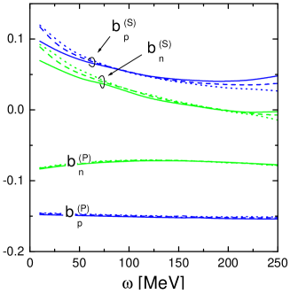
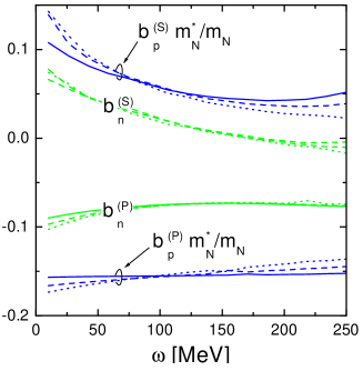
Figure 5: Left panel: Coefficients (44) and (45) of expansion (43) of the regular p-wave part of the polarization operator. Solid, dash and dotted lines show calculations done for nucleon densities $\rho_{n,p}=1,3$, and $5\rho_{0}$, respectively. Right panel: the same as in the left plane but integrals are evaluated with the effective nucleon mass in kinematical prefactors and coefficients $b_{p}^{(S,P)}$ are scaled by $m_{N}^{*}/m_{N}$.

The quantities $b_{n}^{\rm(S,P)}$ and $b_{p}^{\rm(S,P)}$ are shown in Fig. 5 (left plane) for $T=0$ as functions of the kaon energy for several values of the densities $\rho_{i}$. In these calculations integrals ${\rm I}_{\rm S}$ and ${\rm I}_{\rm P}$ have been evaluated with the free nucleon masses. We see that these coefficients are almost density independent and only weakly dependent on the kaon energy in the interval $100~{}{\rm MeV}<\omega<250~{}{\rm MeV}$ of our interest. As we have discussed in the beginning of this section, we replace the baryon masses by the effective masses, as they follow from the mean field solutions, only in the kinematical prefactors in (12,13). The results are shown in the right plane of Fig. 5. The coefficients $b_{n}^{\rm(S,P)}$ depend moderately on the density, as before, whereas the coefficients $b_{p}^{\rm(S,P)}$ exhibit a stronger density dependence, which can be parameterized by the factor $m_{N}/m_{N}^{*}$, as it is demonstrated in Fig. 5. Energy dependence remains to be weak in the interval $100~{}{\rm MeV}<\omega<250~{}{\rm MeV}$ of our interest.

Our result (43) is derived for rather small values of kaon momenta, $\mid\boldsymbol{k}\mid\ll m_{K}$. In order to find the actual value of the p-wave $K^{-}$ condensate amplitude in most general case one needs to deal with momenta up to $\mid\boldsymbol{k}\mid\sim p_{{\rm F},n}\sim m_{K}$. To satisfy the latter general case we extrapolate our result for the regular part of the polarization operator to such momenta. Luckily, within our approach critical points of s- and p-wave condensations deviate not as much from each other, as we will show it, and in this case the kaon condensate momentum in the vicinity of the critical density has extra smallness. Also, the main contribution to the kaon polarization operator comes from the pole terms, which are written explicitly for arbitrary momenta (24). Thereby, ambiguity of mentioned interpolation should not significantly affect our conclusions.

V.2 S-wave Part

The kaon-nucleon interaction determines the following contributions to the s-wave part of the $K^{-}$ meson polarization operator,

$$\Pi_{\rm S}^{(0)}(\omega)={\rm I}_{\rm s-wave}(\omega,0)+\bar{\rm I}_{\rm p-wave}^{\rm reg}(\omega,0)$$

$$+\delta\Pi^{({\rm reg},0)}(\omega)+\Pi^{({\rm pole},0)}(\omega,0)\,,$$ (46)

where the last two terms correspond to non-pole and pole parts of the hyperon exchange terms in the amplitude, respectively. The term $\Pi^{({\rm pole},0)}$ is given by (24). Using (20) we present $\delta\Pi^{({\rm reg},0)}$ as follows

$$\delta\Pi^{({\rm reg},0)}(\omega)\equiv\delta{\rm I}^{\rm reg}_{\rm p-wave}(\omega,0)=\delta{\Pi}_{p\Lambda}^{({\rm reg},0)}(\omega,0)+\delta{\Pi}_{p\Sigma^{0}}^{({\rm reg},0)}(\omega,0)+2\,\delta{\Pi}_{n\Sigma^{-}}^{({\rm reg},0)}(\omega,0),$$

with

$$\delta{\Pi}_{iH}^{({\rm reg},0)}(\omega,0)=-C_{KNH}^{2}\,\times\intop\frac{2{\rm d}^{3}\boldsymbol{p}}{(2\,\pi)^{3}}\frac{(m_{H}^{*}\,\sqrt{s_{0}}-m_{N}^{*\,2}+\omega^{2})(m_{H}^{*}+m_{N}^{*})^{2}}{2\,\epsilon_{i}(p)\sqrt{s_{0}}\,(\sqrt{s_{0}}+m_{H}^{*})}n_{i}(\boldsymbol{p})\,,$$ (47)

where $s_{0}=(\omega+\epsilon_{i}(\boldsymbol{p}))^{2}-\boldsymbol{p}^{2}$, and we also included dependence of effective masses on the mean field. For $T=0$ and for small kaon energies, the integral (47) can be well approximated by the following expression

$$\delta{\Pi}_{iH}^{({\rm reg},0)}(\omega,0)\approx-C_{KNH}^{2}\,\left(\frac{m_{H}^{*2}-m_{N}^{*2}}{2\,m_{N}^{*}}\,\rho^{\rm scal}_{i}+\omega\,\rho_{i}-\frac{\omega^{2}}{m_{H}^{*}+m_{N}^{*}}\,\rho_{i}\right)\,,$$ (48)

where $\rho^{\rm scal}_{i}$ stands for the scalar density of nucleons defined by

$$\rho^{\rm scal}_{i}=\intop_{0}^{p_{{\rm F},i}}\frac{2\,{\rm d}^{3}\boldsymbol{p}}{(2\,\pi)^{3}}\frac{m_{N}^{*}}{\epsilon_{i}(\boldsymbol{p})}\,.$$ (49)

According to (26), (28), the last term in (46) can be cast as

$$\Pi^{({\rm pole},0)}(\omega,0) = {\Pi}_{p\Lambda}^{({\rm pole},0)}(\omega,0)+{\Pi}_{p\Sigma^{0}}^{({\rm pole},0)}(\omega,0)+2\,{\Pi}_{n\Sigma^{-}}^{({\rm pole},0)}(\omega,0),$$ (50)

$$\Pi^{({\rm pole},0)}_{iH}(\omega,0) = C_{KNH}^{2}\,\Big{(}(m_{H}^{*}-m_{N}^{*})^{2}-(\omega+\delta v_{iH})^{2}\Big{)}\,$$

$$\times \frac{(m_{N}^{*}+m_{H}^{*})^{2}}{2\,\pi^{2}}\,\intop\frac{{\rm d}pp^{2}}{\epsilon_{i}(p)[\Delta_{iH}^{+}(\omega,0,\boldsymbol{p})+i0]}n_{i}(\boldsymbol{p}),$$

that follows from (28) at $|\boldsymbol{k}|\rightarrow 0$. The imaginary part, ${\rm Im\,}\Pi^{({\rm pole},0)}_{iH}(\omega,0)$, is given by

$${\rm Im\,}\Pi^{({\rm pole},0)}_{iH}(\omega,0)=-iC_{KNH}^{2}\,\left((m_{H}^{*}-m_{N}^{*})^{2}-(\omega+\delta v_{iH})^{2}\right)\,$$

$$\times\frac{(m_{N}^{*}+m_{H}^{*})^{2}}{8\pi(\omega+\delta v_{iH})^{2}}\sqrt{m_{H}^{*2}-(m_{N}^{*}+\omega+\delta v_{iH})^{2}}\,,$$ (51)

being non-zero for energies $\omega_{iH}^{-}(0)=E_{H}(p_{{\rm F}i})-E_{i}(p_{{\rm F}i})<\omega<\omega_{iH}^{+}(0)=E_{H}(0)-E_{i}(0)$ .

V.3 Energy of the Lowest Branch of the Dispersion Equation at $\boldsymbol{k}\,=0$

In this sub-section we illustrate strength of different terms in (46) applying it to the problem of the s-wave kaon condensation.

The neutron star matter becomes unstable with respect to reactions (1) with the production of the zero-momentum $K^{-}$ meson, when solution ($\omega_{\rm S}=\omega^{\rm min}(\boldsymbol{k})$ at $\boldsymbol{k}=0$) of the dispersion equation

$$\omega_{\rm S}^{2}-m_{K}^{2}-{\rm Re\,}\Pi_{\rm S}(\omega_{\rm S})=0\,$$ (52)

related to the lowest branch of the spectrum, meets the electron chemical potential. Then the s-wave $K^{-}$ condensation may occur by the second-order phase transition.

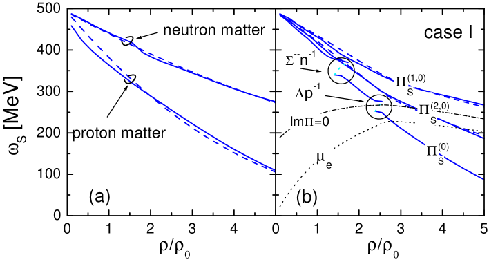
Figure 6: Panel (a): The energy of the lowest $K^{-}$ branch of the dispersion equation (52) at $\boldsymbol{k}=0$ calculated with $\Pi_{\rm S}^{(1,0)}$ (solid lines) for proton and neutron matter. Dash lines present approximate spectra given by (56). Plane (b): The energy of the lowest $K^{-}$ branch of (52) at $\boldsymbol{k}=0$ for real neutron star matter (case I of the hyperon-nucleon interaction) for the s-wave polarization operators $\Pi_{\rm S}^{(1,0)},\Pi_{\rm S}^{(2,0)},\Pi_{\rm S}^{(0)}$ given by (53,54,55) (solid lines). Dash lines are solutions obtained with approximate relations (48,57). Dotted line shows the electron chemical potential. Dash-dotted line depicts the border of the imaginary part of the $K^{-}$ polarization operator (border of hyperonization). Short-dashes show the boarders of the regions of non-physical solutions of (52) characterizing by negative sign residues.

In Fig. 6 we present the energy at the lowest $K^{-}$ branch of the dispersion equation (52), as function of the density at the momentum $\boldsymbol{k}=0$ . The hyperon interaction is taken according to case I. In order to illustrate the strength of different contributions to the s-wave part of the polarization operator (46) we consider several test polarization operators

$$\Pi_{\rm S}^{(1,0)}(\omega) = {\rm I}_{\rm s-wave}(\omega,0)+\bar{\rm I}_{\rm p-wave}^{\rm reg}(\omega,0),$$ (53)

$$\Pi_{\rm S}^{(2,0)}(\omega) = \Pi_{\rm S}^{(1,0)}(\omega)+\delta\Pi^{(\rm reg,0)}(\omega),$$ (54)

$$\Pi_{\rm S}^{(0)}(\omega) = \Pi_{\rm S}^{(2,0)}(\omega)+\Pi^{({\rm pole},0)}(\omega,0).$$ (55)

In panel (a) of Fig. 6 solid lines show the energy of the lowest branch solution of (52) with $\Pi_{\rm S}^{(1,0)}$ for the cases of pure proton and neutron matter. The contribution of $\bar{{\rm I}}_{\rm p-wave}^{\rm reg}(\omega,0)$ is found to be very small, at the level of few percent. It is instructive to compare this our result with that given by the frequently used parameterization of the $K^{-}$ spectrum motivated by the leading-order chiral perturbation theory ($\chi{\rm PT}$) expansion of $K^{-}N$ interaction, cf.  swave-1 ,

$$\omega_{\rm S}^{\chi{\rm PT}}(\rho_{n},\rho_{p})=\sqrt{m_{K}^{2}-S_{K}+V_{K}^{2}}-V_{K}\,,$$

$$S_{K}=\frac{1}{f^{2}}\left(\Sigma_{KN}\,(\rho^{\rm scal}_{p}+\rho^{\rm scal}_{n})+C\,(\rho^{\rm scal}_{p}-\rho^{\rm scal}_{n})\right)\,,\,\,\,\,$$

$$V_{K}=\frac{(2\,\rho_{p}+\rho_{n})}{4\,f^{2}}\,,$$ (56)

where $f\simeq 90$ MeV is the pion decay constant in the chiral limit lk01 , and $\Sigma_{KN}$ and $C$ stand for the isoscalar and isovector kaon-nucleon $\Sigma$-terms related to the explicit chiral symmetry breaking. The SU(3) symmetry predicts $C=m_{K}^{2}\,(2\,m_{\Xi}-3\,m_{\Sigma}+m_{\Lambda})/(16\,(m_{K}^{2}-m_{\pi}^{2}))\approx 66$ MeV, cf. swave . The model polarization operator leading to the dispersion relation (56) can be written as, cf. swave-1 ,

$$\Pi_{\rm S}^{(\chi{\rm PT},0)}(\omega) = -\frac{\Sigma_{KN}}{f^{2}}\,(\rho^{\rm scal}_{p}+\rho^{\rm scal}_{n})-\frac{C}{f^{2}}\,(\rho^{\rm scal}_{p}-\rho^{\rm scal}_{n})$$ (57)

$$- \frac{2\,\rho_{p}+\rho_{n}}{2\,f^{2}}\,\omega\,.$$

Spectrum (56), calculated using $\Sigma_{KN}=150$ MeV, is shown in Fig. 6 (panel (a)) by the dash lines. We observe a good agreement of the model spectrum with that follows from numerical evaluation of the integrals $\Big{[}{\rm I}_{\rm s-wave}(\omega,0)+\bar{{\rm I}}_{\rm p-wave}^{\rm reg}(\omega,0)\Big{]}$. Note, that obtained value of the effective kaon-nucleon $\Sigma$-term is 2–3 times smaller than that used as an ad-hoc parameter in Ref. swave-1 , where the same parameterization (57) has been exploited.

The results for the realistic composition of neutron star matter, shown in Fig. 1, are presented in panel (b) of Fig. 6 for case I of the hyperon-nucleon interaction as a representative example. The solid lines depict the energy at the lowest branch of the dispersion equation calculated for $\boldsymbol{k}=0$ with $\Pi^{(1,0)}_{\rm S}$, $\Pi^{(2,0)}_{\rm S}$ and $\Pi_{\rm S}^{(0)}$. Dash lines show solutions obtained with the approximate expressions (57) in $\Pi_{\rm S}^{(1,0)}$ and (48) for $\delta\Pi^{(\rm reg,0)}$ in $\Pi_{\rm S}^{(2,0)}$. Excellent coincidence of the curves justifies the accuracy of (57) and (48).

Crossing point of the solid and dotted lines corresponds to the critical density of the s-wave condensation for the case of a realistic neutron star composition. We observe that the lines corresponding to $\Pi_{\rm S}^{(1,0)}$ do not meet the chemical potential (dotted line). Therefore, the s-wave kaon-nucleon interaction, following from Ref. lk01 , would not support a second-order phase transition into the s-wave $K^{-}$ condensate state due to the small value of the kaon-nucleon sigma term following from the analysis  lk01 . However, an additional attraction comes from the term $\delta{\rm I}_{\rm p-wave}^{\rm(reg)}$ included in $\Pi_{\rm S}^{(2,0)}$. It makes the reactions (1) possible at density $\geq 4.5\rho_{0}$. Another attractive piece is the pole term ${\rm I}_{\rm p-wave}^{\rm pole}(\omega,0)$ taken into account in $\Pi_{\rm S}^{(0)}$. The significance of these terms, originating both from the hyperon exchange diagram in $\overline{K}N$ interaction, was pointed in Ref. kvk95 . Both mentioned contributions were, however, disregarded in works swave-1 ; swave-2 ; bb ; nscool ; tpl94 ; gs ; pw discussing s-wave $K^{-}$ condensation.

The curves $\omega_{\rm S}$ calculated with the full s-wave polarization operator $\Pi_{\rm S}^{(0)}$ have cuts. In the region between the cuts equation (52) has no solutions with positive residues, cf. kvk95 . The dash-dotted line depicts the border of the imaginary part of the $K^{-}$ polarization operator. We see that, fortunately, within our approach the curve calculated with $\Pi_{\rm S}^{(0)}$ and $\mu_{e}$ meet at energy below the region of the imaginary part. Thus, with the full polarization operator (46), (55) we recovered statement of previous works swave-1 ; swave-2 ; bb ; nscool ; tpl94 ; gs ; pw (where, however, the $2\div 3$ times larger $\Sigma$ term was used) on the possibility of the $K^{-}$ condensate production in reaction (1) at rather moderate densities, $\rho_{\rm c,S}\simeq 2.7\rho_{0}$ in our case. The reader should bear in mind that baryon-baryon correlations are still not included in the above analysis. They will increase $\rho_{\rm c,S}$. This issue will be addressed in section VII.

VI Contributions of the Hyperon Fermi-seas to the Polarization Operator

When nucleon density exceeds the critical density of hyperonization $\rho_{{\rm c},H}$, the Fermi sea of the hyperon $H$ begins to grow, and the $K^{-}$ polarization operator receives new contributions.

VI.1 Pole Terms

New contributions to the $K^{-}$ polarization operator relate to the diagrams (in Schrödinger picture)

$$\parbox{85.35826pt}{ \includegraphics[clip={true},width=85.35826pt]{hyploop.eps} }\,,$$ (58)

where the hyperon and the nucleon interchange their roles compared to the above discussed the hyperon–nucleon-hole $NH$ terms. At finite temperatures these diagrams contribute for all densities. But this contribution is exponentially suppressed for $\rho<\rho_{{\rm c},H}$ and small temperatures.

Account of the hyperon contribution to the pole part of the polarization operator $\Pi^{({\rm pole},0)}$ is simply done with the help of the replacement in (26)

$$\eta^{2}_{iH}\Phi_{iH}(\omega,\boldsymbol{k})\rightarrow\eta^{2}_{NH}\Phi_{iH}(\omega,\boldsymbol{k})+\eta^{2}_{HN}\Phi_{Hi}(-\omega,-\boldsymbol{k})\,,$$ (59)

where the last term implies interchange of all indices $i\leftrightarrow H$ in (27), (28), (34). This replacement results in appearance of an extra term

$$\delta\Pi_{\rm hyp}^{(\rm pole,0)}(\omega,\boldsymbol{k}) = \Pi_{\Lambda p}^{(\rm pole,0)}(-\omega,-\boldsymbol{k})+\Pi_{\Sigma^{0}p}^{(\rm pole,0)}(-\omega,-\boldsymbol{k})$$ (60)

$$+ 2\,\Pi_{\Sigma^{-}n}^{(\rm pole,0)}(-\omega,-\boldsymbol{k}),$$

to be added to the total polarization operator. This term depends on the hyperon density and contributes only at densities $\rho>\rho_{{\rm c},H}$.

VI.2 Regular Terms

There are no any experimental constraints on the hyperon contribution to the regular part of the polarization operator so far. As a rough estimation we may suggest an extension of the model polarization operator (57) to the hyperon sector according to the leading order terms of the chiral Lagrangian

$$\delta\Pi_{{\rm S,hyp}}^{(\chi{\rm PT},0)}(\omega) = -\frac{\Sigma_{KN}}{f^{2}}\,(\rho^{\rm scal}_{\Lambda}+\rho^{\rm scal}_{\Sigma^{-}}+\rho^{\rm scal}_{\Xi^{-}})$$ (61)

$$- \frac{C}{f^{2}}\,(\frac{1}{3}\,\rho^{\rm scal}_{\Lambda}-\rho^{\rm scal}_{\Sigma^{-}}+\rho^{\rm scal}_{\Xi^{-}})$$

$$+ \frac{C_{\Lambda}}{f^{2}}\,\rho^{\rm scal}_{\Lambda}+\frac{\rho_{\Sigma^{-}}+2\,\rho_{\Xi^{-}}}{2\,f^{2}}\,\omega.$$

In this expression we utilize the value of $\Sigma_{KN}$ from the fit with the formula (56) to the numerical results in Fig. 6 ($\Sigma_{KN}\simeq 150$ MeV), whereas the values of coefficients $C\approx 66$ MeV and $C_{\Lambda}=m_{K}^{2}\,(m_{\Xi}-m_{\Lambda})/(12\,(m_{K}^{2}-m_{\pi}^{2}))\approx 34$ MeV and $f\simeq 90$ MeV are predicted by the chiral SU(3) symmetry. To estimate the non-pole contribution from the nucleon u-channel exchange (analogous to $\delta\Pi^{(\rm reg,0)}$) we use approximate relations (48)

$$\delta\Pi_{\rm S,hyp}^{({\rm reg},0)}(\omega)=-C_{KN\Lambda}^{2}\,$$

$$\times\left[\frac{m_{N}^{*2}-m_{\Lambda}^{*2}}{2\,m_{\Lambda}^{*}}\,\rho^{\rm scal}_{\Lambda}-\omega\,\rho_{\Lambda}-\frac{\omega^{2}}{m_{\Lambda}^{*}+m_{N}^{*}}\,\rho_{\Lambda}\right]$$

$$\qquad\qquad\qquad\,\,-2\,C_{KN\Sigma}^{2}$$

$$\times\left[\frac{m_{N}^{*2}-m_{\Sigma}^{*2}}{2\,m_{\Sigma}^{*}}\,\rho^{\rm scal}_{\Sigma^{-}}-\omega\,\rho_{\Sigma^{-}}-\frac{\omega^{2}}{m_{\Sigma}^{*}+m_{N}^{*}}\,\rho_{\Sigma^{-}}\right]\,.$$ (62)

With this estimation we do not take into account contributions to the regular p-wave part of the polarization operator $\propto\boldsymbol{k}^{2}\,\rho_{H}$.

VI.3 Energy of the Lowest Branch of the Dispersion Equation at $\boldsymbol{k}=0$

Solutions related to the lowest branch of the dispersion equation (52) for $\boldsymbol{k}=0$ calculated with the polarization operator

$$\Pi_{{\rm S},{\rm hyp}}^{(0)}(\omega) = \Pi_{\rm S}^{(0)}(\omega)+\delta\Pi_{{\rm S},{\rm hyp}}^{(0)}(\omega),$$

$$\delta\Pi_{{\rm S},{\rm hyp}}^{(0)}(\omega) = \delta\Pi_{{\rm S},{\rm hyp}}^{(\chi{\rm PT},0)}(\omega)+\delta\Pi^{({\rm reg},0)}_{\rm hyp}(\omega)$$ (63)

$$+ \delta\Pi^{({\rm pole},0)}_{\rm hyp}(\omega,0)\,$$

are shown in Fig. 7 by solid lines in comparison with corresponding solutions obtained without inclusion of hyperons (dash lines). Calculations are done for hyperon coupling constants corresponding to case I. We see that presence of hyperons produces an additional small attraction only at rather high densities ($>4\rho_{0}$). The reasons are partial cancellation of the attractive $\Pi_{{\rm S},{\rm hyp}}^{(\chi{\rm PT},0)}$ term and the repulsive $\delta\Pi^{(\rm reg,0)}_{\rm hyp}$ term and that in the framework of our model for description of the neutron star matter hyperon concentrations are much smaller than the neutron concentration and even smaller than the proton one. Thus, population of the hyperon Fermi seas only slightly affects the s-wave part of the polarization operator.

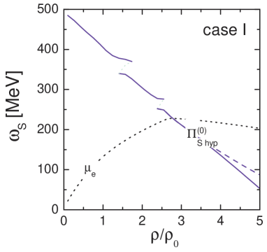
Figure 7: The energy of the lowest branch of the dispersion equation at $\boldsymbol{k}=0$ calculated with the polarization operator $\Pi_{\rm S,hyp}^{(0)}$ given by (63) is depicted by solid lines. Dashed line shows the corresponding solution with the polarization operator (55). The dotted line depicts the electron chemical potential.

This allows us not to care much about the hyperon Fermi sea occupations considering $\boldsymbol{k}=0$ case.

VII Baryon-Baryon Correlations

Operating with the polarization operator constructed by integrating the meson-nucleon scattering amplitude over the nucleon Fermi sea, e.g., as in (12,13), one assumes that all multiple meson-nucleon interactions are independent from each other and have the same probability proportional to the nucleon local density $\rho(\boldsymbol{r\,})$. However the successive meson-nucleon scatterings in dense nuclear matter are not independent because of the core of nucleon-nucleon interactions and the Pauli exclusion principle Bruk ; jb78 . The probability to find two nucleons $i$ and $i^{\prime}$ at the positions $\boldsymbol{r}_{1}$ and $\boldsymbol{r}_{2}$, respectively, is proportional to the two-particle density

$$\rho_{ii^{\prime}}(\boldsymbol{r}_{1},\boldsymbol{r}_{2})=[1+C_{ii^{\prime}}(|\boldsymbol{r}_{1}-\boldsymbol{r}_{2}\,|)]\,\rho_{i}(\boldsymbol{r}_{1}\,)\,\rho_{i^{\prime}}(\boldsymbol{r}_{2}\,)$$

with the correlation function $C_{ii^{\prime}}(r)<0$ and is, therefore, reduced in comparison to the product of two single particle densities. The correlation function can be approximately written as

$$C_{ii^{\prime}}(r)\approx C^{\rm core}(r)+\delta_{ii^{\prime}}\,C^{\rm Pauli}_{i}(r)\,[1+C^{\rm core}(r)]$$ (64)

with contributions from the hard core, $C^{\rm core}$, and the Pauli exclusion principle, $C^{\rm Pauli}$, assuming that both correlations contribute multiplicatively. The former can be taken from the description of nuclear matter with the realistic nucleon-nucleon interaction. The convenient parameterization was suggested in Ref. bbow , $C^{\rm core}(r)\approx-j_{0}(m_{0}\,r)$ with $m_{0}\approx 5.6m_{\pi}$, where $j_{l}(x)$ stands for the spherical Bessel function. For the Pauli correlation we use expression for the ideal fermion gas FW , $C^{\rm Pauli}_{i}(r)=-9\,j_{1}^{2}(p_{{\rm F}i}r)/(2\,p_{{\rm F}i}^{2}r^{2})$ .

VII.1 Correction of s-wave and Regular p-wave Terms

General derivation of the corrections to the meson propagation in dense nuclear matter due to the nucleon-nucleon correlations (so-called Ericson-Ericson-Lorentz-Lorenz corrections) can be found in Ref. ee66 ; f73 for pions. In Ref. corr-pand ; wrw97 it was extended for kaons.

In diagrams, correlation processes can be presented by symbolic equation

$$\parbox{170.71652pt}{ \includegraphics[width=170.71652pt,clip={true}]{reg-cor-B.eps}}\quad,$$ (65)

where the wavy line relates to the kaon, the sum goes over the baryon species. The line without arrow means that both particles and holes are treated on equal footing (the conservation of charges, e.g. strangeness, baryonic number etc., in each vertex is implied). The hatched triangle is the bare scattering amplitude (scattering on the particle or on the hole) and the full triangle stands for the amplitude including baryon-baryon correlations. The dotted line symbolically depicts the two-baryon correlation function $C_{BB^{\prime}}$ due to the $BB^{\prime}$ correlations through the core and the Pauli principle. There are nor experimental information neither theoretical estimations for the hyperon-nucleon and hyperon-hyperon correlations. Since the latter ones are less relevant for our discussion below we will neglect them. Thus we actually include only minimal correlations given by $C_{ii^{\prime}}$ nucleon-nucleon correlation functions.

We consider first the correlation corrections to the s-wave part of the kaon polarization operator, $\Pi_{\rm S}^{(0)}$ given by (46), and the regular p-wave part , $\Pi_{\rm P}^{({\rm reg},0)}$ from (43). We separate contributions induced by the scattering on a nucleon of a given isospin species $i=\{n,p\}$.

$$\Pi_{\rm S}^{(0)}(\omega) = \Pi_{{\rm S},n}^{(0)}(\omega)+\Pi_{{\rm S},p}^{(0)}(\omega)\,,$$

$$\Pi_{{\rm S},i}^{(0)}(\omega) = {\rm I}_{{\rm s-wave},i}(\omega,0)+{\rm I}_{{\rm p-wave},i}(\omega,0),$$

cf. (12,13). Then, adopting results of Refs. w77 ; wrw97 we may present the polarization operator terms corrected by baryon-baryon correlations as

$$\Pi_{\rm S}(\omega)=\frac{\widetilde{\Pi}_{{\rm S},n}(\omega)+\widetilde{\Pi}_{{\rm S},p}(\omega)+2\,\widetilde{\Pi}_{{\rm S},n}(\omega)\,\widetilde{\Pi}_{{\rm S},p}(\omega)\,\xi_{pn}^{\rm(S)}(\omega)}{1-\widetilde{\Pi}_{{\rm S},n}(\omega)\,\widetilde{\Pi}_{{\rm S},p}(\omega)\,(\xi_{pn}^{\rm(S)}(\omega))^{2}}\,,\qquad\widetilde{{\Pi}}_{{\rm S},i}(\omega)=\frac{{\Pi}_{{\rm S},i}^{(0)}(\omega)}{1-\xi_{ii}^{\rm(S)}(\omega)\,{\Pi}_{{\rm S},i}^{(0)}(\omega)}\,,$$ (66)

$$\Pi_{\rm P}^{\rm reg}(\omega,\boldsymbol{k})=\boldsymbol{k}^{2}\,\frac{\widetilde{b}_{p}(\omega)+\widetilde{b}_{n}(\omega)\,+2\,\widetilde{b}_{p}(\omega)\,\widetilde{b}_{n}(\omega)\xi^{\rm(P)}_{np}(\omega)}{1-\widetilde{b}_{p}(\omega)\,\widetilde{b}_{n}(\omega)(\xi_{np}^{\rm(P)}(\omega))^{2}}\,,\qquad\widetilde{b}_{i}(\omega)=\frac{b_{i}(\omega)\,(\rho_{i}/\rho_{0})}{1-b_{i}(\omega)\,\rho_{i}\,\xi_{ii}^{\rm(P)}(\omega)/\rho_{0}}\,.$$ (67)

Functions, $\xi_{ii^{\prime}}^{\rm(S)}$ and $\xi_{ii^{\prime}}^{\rm(P)}$ are defined as, cf. Ref. wrw97 ,

$$\xi_{ii^{\prime}}^{\rm(S)}(\omega) = \intop{\rm d}^{3}rC_{ii^{\prime}}(r)\,D_{K}^{0}(\omega,r)\,,$$ (68)

$$\xi_{ii^{\prime}}^{\rm(P)}(\omega) = \frac{1}{3}\,\intop{\rm d}^{3}rC_{ii^{\prime}}(r)\,\nabla^{2}\,D_{K}^{0}(\omega,r)$$ (69)

$$= -\frac{1}{3}\,\Big{(}C_{ii^{\prime}}(0)-(m_{K}^{2}-\omega^{2})\,\xi_{ii^{\prime}}^{\rm(S)}(\omega)\Big{)}\,,$$

containing Pauli and core contributions following (64), $i,i^{\prime}=\{n,p\}$, and $D_{K}^{0}(\omega,r)=-\exp(-\sqrt{m_{K}^{2}-\omega^{2}}\,r)/(4\,\pi\,r)$, as the free kaon propagator in the ”mixed” representation.

Using (65) one finds that the repulsive core contributes with

$$\xi_{ii^{\prime}}^{\rm(P,\,core)}=\xi_{K}^{\rm(P,\,core)}(\omega)=\frac{1}{3}\,\frac{m_{0}^{2}}{(m_{0}^{2}+m_{K}^{2}-\omega^{2})}$$ (70)

to the p-wave $\xi$’s and with

$$\xi_{ii^{\prime}}^{\rm(S,\,core)}=\xi_{K}^{\rm(S,\,core)}(\omega)=\frac{1}{(m_{0}^{2}+m_{K}^{2}-\omega^{2})}$$ (71)

to the s-wave ones. The contribution from Pauli spin-correlation (second term in $C_{ii^{\prime}}$) to the p-wave correlation function $\xi^{\rm(P)}_{ii}$ is shown in Fig. 8 (left panel) as a function of the Fermi momentum for different kaon energies. We see that the correlation parameter decreases with density since the baryon-baryon correlations hold baryons apart from each other and suppress, thereby, effect of the Pauli exclusion principle. The right panel of Fig. 8 presents the values of the correlation function (68, 69) calculated for $\omega=\mu_{e}$ in the neutron star matter with the hyperon coupling constants according to case I.

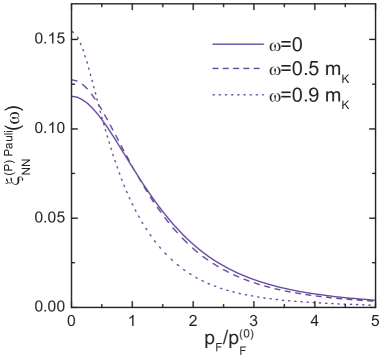
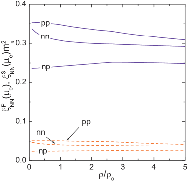
Figure 8: Left panel: contribution of the Pauli spin-correlations to the p-wave correlation function (69) vs. the Fermi momentum for different kaon energies, $p_{\rm F}^{(0)}$ is the Fermi momentum for $\rho=\rho_{0}$. Right Panel: the s-wave (dash lines) and p-wave (solid lines) correlation functions (68,69) evaluated for $\omega=\mu_{e}$ in neutron star matter (case I) as function of the total baryon density.

We leave the contributions from the hyperon Fermi seas to the regular part of the polarization operator, $\delta\Pi_{\rm S,hyp}^{(0)}$, without corrections due to the baryon-baryon correlations in view of their small contributions.

VII.2 Correction of p-wave Pole Terms

We turn now to consideration of effect of correlations in the particle-hole channel.

If we approximate the free $\overline{K}N$ scattering amplitude (hatched triangle) in (65) by the hyperon-exchange diagram, the same one, which produces the particle-hole diagrams (25), we can see that the account of correlations via (65) is equivalent to the replacement 

(72)

with a modified vertex (fat point) obeying equation

$$\parbox{219.08612pt}{ \includegraphics[clip={true},width=219.08612pt]{vert.eps}}\,,$$ (73)

where the particle-hole irreducible box ${T}_{HN^{\prime}}^{\rm loc}$ (light square) can be expressed in terms of $\xi^{\rm P}$ and kaon-nucleon-hyperon coupling constants.

Below we would like to put the discussion on a more phenomenological level. According to the argumentation of the Fermi-liquid theory tkfs , the particle-hole irreducible box ${T}_{HN^{\prime}}^{\rm loc}$ has a weak dependence on incoming energies and momenta and can be, therefore, parameterized in terms of phenomenological Landau-Migdal parameters:

$${T}_{\Lambda{N}}^{\rm loc} = \parbox{56.9055pt}{ \includegraphics[width=56.9055pt,clip={true}]{diag-tln.eps}}=C_{0}\,f^{\prime}_{\Lambda}\,s_{12}\,,\qquad\qquad{T}_{\Sigma{N}}^{\rm loc}=\parbox{56.9055pt}{ \includegraphics[width=56.9055pt,clip={true}]{diag-tsn.eps}}=C_{0}\,g^{\prime}_{\Sigma}\,s_{12}\,{P}_{\Sigma{\rm N}}^{(1/2)}\,,$$

$${T}_{\Lambda\Sigma^{\alpha}}^{\rm loc} = \parbox{56.9055pt}{ \includegraphics[width=56.9055pt,clip={true}]{diag-tls.eps}}=C_{0}\,f^{\prime}_{\Lambda\Sigma}\,s_{12}\,\tau^{\alpha}\,,\qquad{T}_{\Sigma^{*\alpha}\rm N}^{\rm loc}=\parbox{56.9055pt}{ \includegraphics[width=56.9055pt,clip={true}]{diag-tssn.eps}}=C_{0}\,g^{\prime}_{\Sigma^{*}}\,S_{12}\,{P}_{\Sigma^{*}{\rm N}}^{(1/2)}\,,$$ (74)

with $\alpha=1,2,3$. The amplitudes are normalized with $C_{0}=300\,{\rm MeV}\cdot{\rm fm}^{3}$, that allows to compare the values for the hyperon-nucleon correlation parameters with those for the nucleon-nucleon correlations introduced in Ref. MSTV90 . In (74) ${P}_{\Sigma N}^{(1/2)}=(1-\boldsymbol{t}_{\Sigma}\cdot\boldsymbol{\tau})/3$ is the projection operator onto the given $\Sigma N$ state with isospin $1/2$, $\boldsymbol{t}_{\Sigma}$ are the isospin-1 matrices and $\boldsymbol{\tau}$ are the Pauli matrices of the nucleon isospin, as above. The projector ${P}_{\Sigma^{*}{\rm N}}^{(1/2)}$ is defined analogously. The spin-spin operators in the particle-hole channel are given by $s_{12}=(\boldsymbol{\sigma}_{1}\boldsymbol{\sigma}_{2})$, and $S_{12}=(\boldsymbol{S}_{1}\boldsymbol{S_{2}}^{\dagger})$, with $\boldsymbol{S}$ standing for spin-operator, which couples spin 1/2 and 3/2 states.

The inclusion of correlations according to (73) brings the pole polarization operator (24) into the form

$${\Pi}^{\rm pole}(\omega,\boldsymbol{k}) = \frac{\widetilde{\Pi}_{p\Lambda}(\omega,\boldsymbol{k})+\widetilde{\Pi}_{\Sigma}(\omega,\boldsymbol{k})+2\,c\,f^{\prime}_{\Lambda\Sigma}\,\widetilde{\Pi}_{p\Lambda}(\omega,\boldsymbol{k})\,\widetilde{\Pi}_{\Sigma}(\omega,\boldsymbol{k})/3}{1-c^{2}\,f^{{}^{\prime}2}_{\Lambda\Sigma}\,\widetilde{\Pi}_{p\Lambda}(\omega,\boldsymbol{k})\,\widetilde{\Pi}_{\Sigma}(\omega,\boldsymbol{k})/3}+{\Pi}_{\Sigma^{*}}(\omega,\boldsymbol{k})\,,$$

$$\widetilde{\Pi}_{p\Lambda}(\omega,\boldsymbol{k}) = \frac{\Pi^{\rm(0)}_{p\Lambda}(\omega,\boldsymbol{k})}{1-f^{\prime}_{\Lambda}\,C_{0}\,\Phi_{p\Lambda}(\omega,\boldsymbol{k})}\,,\qquad c=C_{0}/(C_{KN\Lambda}\,C_{KN\Sigma}),$$

$$\widetilde{\Pi}_{\Sigma}(\omega,\boldsymbol{k}) = \frac{\Pi^{\rm(0)}_{p\Sigma^{0}}(\omega,\boldsymbol{k})+2\,\Pi^{\rm(0)}_{n\Sigma^{-}}(\omega,\boldsymbol{k})}{1-g^{\prime}_{\Sigma}\,C_{0}\,(\Phi_{p\Sigma^{0}}(\omega,\boldsymbol{k})+2\,\Phi_{n\Sigma^{-}}(\omega,\boldsymbol{k}))/3}\,,$$

$${\Pi}_{\Sigma^{*}}(\omega,\boldsymbol{k}) = \frac{\Pi^{\rm(0)}_{p\Sigma^{*0}}(\omega,\boldsymbol{k})+2\,\Pi^{\rm(0)}_{n\Sigma^{*-}}(\omega,\boldsymbol{k})}{1-g^{\prime}_{\Sigma^{*}}\,C_{0}\,(\Phi_{p\Sigma^{*0}}(\omega,\boldsymbol{k})+2\,\Phi_{n\Sigma^{*-}}(\omega,\boldsymbol{k}))/3}\,.$$ (75)

VII.3 Correlation Parameters

To our best knowledge there is no direct experimental information on the values of the Landau-Migdal parameters for the hyperon-nucleon interactions $f^{\prime}_{\Lambda}$, $g^{\prime}_{\Sigma(\Sigma^{*})}$, and $f^{\prime}_{\Lambda\Sigma}$. In principle, this information could be extracted from the data on multi-strange hyper-nuclei, which, however, are rather poor, if not absent. In the work kv98 the Landau-Migdal parameter $f^{\prime}_{\Lambda}$ was estimated in line with Refs. correst , where Landau-Migdal parameters of the nucleon-nucleon interaction were calculated within Ericson-Ericson-Lorentz-Lorenz approach. We will follow this approach, estimating these parameters. Further corrections can be computed, as in Ref. bbow .

Following correst we assume that the squared block in (74) is determined by exchanges of the kaon and the heavy strange vector meson $K^{*}$ with the mass $m_{K^{*}}\simeq 892$ MeV. This can be shown in diagrams as

$$\parbox{199.16928pt}{ \includegraphics[width=199.16928pt,clip={true}]{tloc.eps}}\,\,.$$ (76)

Intermediate states in the processes (76), (65) involve large momenta suppressing medium effects. In this approximation, correlation parameters are equal for $HN^{-1}$ and $NH^{-1}$, for the nucleon and the hyperon of given species. Then, including hyperon Fermi seas, the pole term of the polarization operator is corrected with the help of the replacement (59) in (75). The block (76), being evaluated at zero momentum and energy transfer, contributes to the local interaction in (74) as

$$T_{HN}^{\rm loc} \approx C_{KNH}\,C_{KNH}\,\xi^{\rm(P,\,core)}_{K}(0)$$

$$+ C_{K^{*}NH}\,C_{K^{*}NH}\,\xi^{\rm(P,\,core)}_{K^{*}}(0)\,,$$

$$\qquad H=\Lambda,\Sigma,\Sigma^{*}\,,$$

$$T_{\Lambda\Sigma}^{\rm loc}(\omega) \approx C_{KN\Lambda}\,C_{KN^{\prime}\Sigma}\,\xi^{\rm(P,\,core)}_{K}(0)$$ (78)

$$+ C_{K^{*}N\Lambda}\,C_{K^{*}N^{\prime}\Sigma}\,\xi^{\rm(P,\,core)}_{K^{*}}(0)\,\,.$$

For shortness we do not write here explicitly the spin and isospin operators which are exactly the same as in (74). The vector meson coupling constants $C_{K^{*}NH}$ in (VII.3) correspond to the non-relativistic vertex $\propto[\boldsymbol{\sigma}\times\boldsymbol{k}]$. Coupling constants can be, e.g., taken from the analysis of the Jülich model of the hyperon-nucleon interaction via the meson exchange Julich : $C_{K^{*}N\Lambda}=-\frac{1.3}{m_{\pi}}$ , $C_{K^{*}N\Sigma}=\frac{0.07}{m_{\pi}}$ , and $C_{K^{*}N\Sigma^{*}}=\frac{0.7}{m_{\pi}}$ . These values account for the form-factors used in Julich . In particular, the form-factor related to a very soft energy range is responsible for a strong suppression of the $C_{K^{*}N\Sigma}$ vertex.

Thus, the Landau-Migdal correlation parameters (74) can be cast as

$${C_{0}}f^{\prime}_{\Lambda} = {C_{KN\Lambda}^{2}}\,\left[\xi_{K}^{\rm(P,\,core)}(0)+R_{\Lambda\Lambda}\,\xi_{K^{*}}^{\rm(P,\,core)}(0)\right]\,,$$

$${C_{0}}g^{\prime}_{\Sigma} = 3\,{C_{KN\Sigma}^{2}}\,\left[\xi_{K}^{\rm(P,\,core)}(0)+R_{\Sigma\Sigma}\,\xi_{K^{*}}^{\rm(P,core)}(0)\right]\,,$$

$${C_{0}}f^{\prime}_{\Lambda\Sigma} = {C_{KN\Lambda}\,C_{KN\Sigma}}\,\left[\xi_{K}^{\rm(P,\,core)}(0)+R_{\Lambda\Sigma}\,\xi_{K^{*}}^{\rm(P,\,core)}(0)\right]\,,$$

$${C_{0}}g^{\prime}_{\Sigma^{*}} = 3\,{C_{KN\Sigma^{*}}^{2}}\,\left[\xi_{K}^{\rm(P),\,core}(0)+R_{\Sigma^{*}\Sigma^{*}}\,\xi_{K^{*}}^{\rm(P),\,core}(0)\right)]\,,$$

where the first term was introduced in (70), $\xi_{K}^{\rm(P,\,core)}(0)\simeq 0.24$, the second one is equal to $\xi_{K^{*}}^{\rm(P,\,core)}(0)=\frac{2}{3}\,m_{0}^{2}/(m_{0}^{2}+m_{K^{*}}^{2})\simeq 0.28$, cf. correst , $R_{HH^{\prime}}=C_{K^{*}NH}\,C_{K^{*}NH^{\prime}}/(C_{KNH}\,C_{KNH^{\prime}})$ with $R_{\Lambda\Lambda}\simeq 3.7$, $R_{\Sigma\Sigma}\simeq 0.04$, $R_{\Lambda\Sigma}\simeq 0.39$, and $R_{\Sigma^{*}\Sigma^{*}}\simeq 0.69$. Additional factor 2 in $\xi^{\rm(P,\,core)}_{K^{*}}$ compared to $\xi^{\rm(P,\,core)}_{K}$, originates from the reduction $[\boldsymbol{\sigma}_{2}\times\boldsymbol{k}]\,[\boldsymbol{\sigma}_{1}\times\boldsymbol{k}]\to s_{12}$. Finally, we estimate the following values of the correlation parameters in (74) as

$$f^{\prime}_{\Lambda}\simeq 0.9\,,\quad g^{\prime}_{\Sigma}\simeq 0.1\,,\quad f^{\prime}_{\Lambda\Sigma}\simeq-0.1\,,\quad g^{\prime}_{\Sigma^{*}}\simeq 1.2\,.$$ (79)

Compared to kv98 we obtained a smaller value of the corresponding parameter $C_{0}f^{\prime}_{\Lambda}\simeq 0.6/m_{\pi}^{2}$, since we included here the form-factors mentioned above .

VII.4 Energy of the Lowest Branch of the Dispersion Relation at $\boldsymbol{k}\,=0$.

Fig. 9 illustrates how much baryon-baryon correlations affect the terms of the bare polarization operator. For case I we show the energy of the lowest branch of the dispersion equation at $\boldsymbol{k}=0$ calculated with the polarization operator ${\Pi}_{\rm S}^{(2)}$ constructed from ${\Pi}_{\rm S}^{(2,0)}$ according to (66) and the polarization operator ${\Pi}_{\rm S}(\omega)={{\Pi}}_{\rm S}^{(2)}(\omega)+{\Pi}^{\rm pole}(\omega,0)$, where ${\Pi}^{\rm pole}(\omega,0)$ follows from (75) with parameters (79).

At $\rho>\rho_{c,H}$ we have to include correlations in the term $\delta\Pi_{\rm S,hyp}^{(0)}$ in (63). The pole term $\delta{\Pi}^{(\rm pole,0)}_{\rm hyp}(\omega,0)$ is included in (75) with the help of the replacement (59). The other terms $\delta\Pi_{\rm S,hyp}^{(\chi{\rm PT},0)}(\omega)$ and $\delta{\Pi}_{{\rm S},h}^{(0)}$ can be corrected in the same manner as the ${\Pi}_{{\rm S}}^{(0)}$ term. However these terms are rather small as it is demonstrated by Fig. 7. Therefore we omit correlations in them in further.

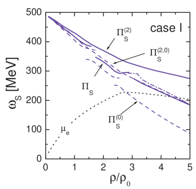
Figure 9: Solid lines present the energy of the lowest branch of the dispersion equation at $\boldsymbol{k}=0$ calculated with the polarization operators ${\Pi}_{{\rm S}}^{(2)}$ and ${\Pi}_{{\rm S}}$ including effects of baryon-baryon correlations. Dash-dotted continuations of solid curves demonstrate effect of the filling of the hyperon Fermi seas on the s-wave polarization operator. Correlation parameters are taken according to Fig. 8 (right panel), (68) and (79). Dashed lines show solutions ${\Pi}_{\rm S}^{(2,0)}$ and ${\Pi}_{\rm S}^{(0)}$ without correlation effects, as in Fig 6, plane (b). The dotted line depicts the electron chemical potential.

From Fig. 9 we see that baryon-baryon correlations suppress the s-wave part of the polarization operator, in agreement with the statements corr-pand ; wrw97 . It results in an increase of the critical density of the s-wave condensation, from $2.7\rho_{0}$ to $4.3\rho_{0}$ for case I chosen by us for an illustration.

VIII $K^{-}$ Condensation in Neutron Stars

In sections IV-VII we have constructed the $K^{-}$ polarization operator. Now we use it to study a possible instability of the system with respect to a phase transition into a state with $K^{-}$ condensate.

For this aim we first investigate solutions of the $K^{-}$ dispersion relation

$$\omega^{2}-\boldsymbol{k}^{2}-m_{K}^{2}-{\rm Re\,}\Pi^{\rm tot}(\omega,\boldsymbol{k})=0,$$ (80)

where the complete polarization operator is given by

$$\Pi^{\rm tot}(\omega,\boldsymbol{k}) = \Pi_{{\rm S}}(\omega)+\Pi^{\rm reg}_{{\rm P}}(\omega,\boldsymbol{k})+\Pi^{\rm pole}_{\rm P}(\omega,\boldsymbol{k})$$ (81)

$$+ \delta\Pi_{\rm hyp}^{(\chi{\rm PT},0)}(\omega)+\delta\Pi_{\rm hyp}^{\rm reg,0}(\omega)\,.$$

It contains the s-wave part, regular p-wave and pole parts of the polarization operator given by (66,67) and (75), respectively, and the terms determined by the hyperon populations (61) and (62). The correlation parameters are taken according to (68,69) and (79).

There are two different possibilities. The $K^{-}$ condensation may occur in the neutron star matter via a second-order phase transition or a first-order phase transition. The dynamics of both phase transitions are quite different. Therefore, both possibilities might be realized at different physical conditions related to the different stages of neutron star evolution.

In the case of a second-order phase transition, at the moment, when the density in the neutron star center achieves the critical density $\rho_{c}^{\rm II}$, the reactions (1) come into the game. At this second order phase transition the isospin composition and the density may change only soothly. For typical times $\tau\propto\tau_{\rm react}\sqrt{\rho_{c}^{\rm II}}/\sqrt{\rho-\rho_{c}^{\rm II}}$ the system creates an energetically favorable condensate state, $\tau_{\rm react}$ is the typical time of weak processes (1). The condensate appears within the region where $\rho>\rho_{c}^{\rm II}$. If it happens during the supernova explosion, the typical size of the condensate region might become of the order of the neutron star radius. Due to the energy conservation the positive energy is released in such a transition. When the condensate region is heated up to the temperatures $T\geq T_{\rm opac}\sim(1\div 2)$ MeV neutrinos are trapped. At this stage the cooling time is determined by the neutrino heat transport from the condensate interior of the neutron star to its exterior MSTV90 . When the star cools down to smaller temperatures, $T<T_{\rm opac}$, the neutron star begins to be transparent for neutrinos. They can be directly radiated away. A part of the energy is radiated by photons from the star surface. In binary long lived systems the critical density in the neutron star center can be achieved by the accretion process. Then the transition is characterized by the typical large time of the accretion.

In the case of a first-order phase transition the final state might significantly differ from the initial one by its isospin composition and the density. Thus this new state can’t be prepared in microscopic processes. Too small droplets of the new phase are not energetically favorable due to a positive surface energy contribution. When the density in the star center begins to exceed the value $\rho_{c}^{\rm I}<\rho_{c}^{\rm II}$ the system arrives at a metastable state. When in a fluctuation a droplet of the new phase (with density $\rho_{c}^{\rm fin}>\rho_{c}^{\rm I}$) of rather large (overcritical) size is prepared it starts to grow. At zero temperature, the probability of the creation of such a droplet via quantum fluctuations is very small but increases greatly with the temperature MSTV90 . Thus, the first-order phase transition occurs most likely at an initial stage of the neutron star formation or cooling when the temperature is rather large. If the density in the center of a star exceeds the value $\rho_{c}^{\rm II}$, a second-order phase transition may also occur. In binary stellar systems, where the neutron star slowly accretes the mass from the star-companion and the temperature is small, the second-order phase transition might be a more probable one (depending on the accretion rate).

VIII.1 II Order Phase Transition to the s-wave Condensate State

Let us first analyze possibility of the s-wave $K^{-}$ condensation.

In Fig. 10, summarizing the results of sections V.3, VI.3, VII.4, we show the energy of the lowest $K^{-}$ branch of the kaon dispersion relation (80) for $\boldsymbol{k}=0$ together with the electron chemical potential. For the given parameter choice (see different panels), the crossing points of the lines indicate the critical density of the s-wave condensation via the second order phase transition.

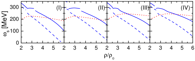
Figure 10: The energy of the lowest $K^{-}$ branch of the dispersion relation (80) for $\boldsymbol{k}=0$ is depicted by solid lines. The dotted lines show the electron chemical potentials. The dashed lines are calculated without baryon-baryon correlations. Different panels correspond to the interaction given by the cases I-IV.

We see that for all the models the neutron star matter is unstable with respect to reactions (1) in the density interval $(3\div 5.2)\rho_{0}$ in dependence on the choice of the correlation parameters and the parameters of the hyperon-nucleon interactions. Recall, that in the framework of our model the attraction due to the s-wave kaon-nucleon interaction corresponds to the effective kaon-nucleon sigma term $\Sigma_{KN}$ equal to 150 MeV, which is much smaller than the value $\Sigma_{KN}\simeq(300\div 400)$ MeV used in the previous works studying the s-wave $K^{-}$ condensation. Additional suppression comes from the nucleon-nucleon correlations. Nevertheless, we found also an extra attraction associated with $\delta\Pi^{\rm reg}$, $\Pi^{\rm pole}$ and $\delta\Pi_{h}$ terms. Thus, until correlations are not included, we support a conjecture of previous works on the possibility of the s-wave condensation at $\rho_{\rm c,S}^{\rm(II)}\sim 3\rho_{0}$. However, the baryon-baryon correlations additionally shift the condensation critical density to larger values than those ones discussed in Refs. swave-1 ; swave-2 ; bb ; nscool ; tpl94 ; gs ; pw .

Note that here we checked the necessary condition of the $s$-wave condensation but we did not yet minimize the energy of the lowest branch of the dispersion equation, $\omega^{\rm min}(\boldsymbol{k})$, over $|\boldsymbol{k}|$. Thus we still can’t conclude whether we deal with the s-wave or the p-wave condensation.

VIII.2 II Order Phase Transition to the p-wave Condensate State

In this section we are going to study the principal possibility of the p-wave $K^{-}$ condensation in neutron star matter at the assumption of the second order phase transition. We would like to investigate whether the p-wave condensation second order phase transition can occur at densities smaller than that for the s-wave condensation, and how much such a situation is sensitive to the parameter choices for hyperon-nucleon interactions and correlations.

Let us first assume that the s-wave $K^{-}$ condensation is indeed possible at some critical density $\rho_{\rm c,S}$. The lowest energy branch of the $K^{-}$ spectrum at small momenta is given by

$$\omega\approx\omega_{{\rm S}}+\alpha(\omega_{{\rm S}})\,Z_{\rm S}(\omega_{\rm S})\,\boldsymbol{k}^{\,2}\,,$$ (82)

where $\omega_{\rm S}$ is, as before, $\omega(\boldsymbol{k}=0)$ for the lowest energy branch of the dispersion law given by the solution of the equation $\omega_{\rm S}^{2}=m_{K}^{2}+{\rm Re\,}\Pi_{\rm S}(\omega_{\rm S},\boldsymbol{k}=0)$, and

$$Z^{-1}_{\rm S}(\omega) = \left(2\,\omega_{\rm S}-\frac{\partial{\rm Re\,}\Pi_{\rm S}(\omega,\boldsymbol{k})}{\partial\omega}\Big{|}_{\boldsymbol{k}=0}\right)>0\,,$$

$$\alpha(\omega) = 1+\frac{\partial{\rm Re\,}\Pi_{\rm P}(\omega,\boldsymbol{k})}{\partial\boldsymbol{k}^{\,2}}\Big{|}_{\boldsymbol{k}=0}\,.$$

If $\alpha(\omega_{\rm S})<0$ at $\rho_{\rm c,S}$, then instead of the s-wave condensation we, actually, have the p-wave condensation at a somewhat smaller density. The aim of this section is to find the value $\alpha(\omega_{\rm S})$ in (82) at the critical point of the s-wave condensation i.e., when $\omega_{\rm S}=\mu_{e}$.

Taking into account the p-wave kaon-baryon interaction which we have determined in Sect. V, we find

$$\alpha(\omega)=1+\alpha_{\rm pole}(\omega)+\alpha_{\rm reg}(\omega)\,.$$ (83)

Without baryon-baryon correlations, the contribution of the pole part is

$$\alpha_{\rm pole}^{(0)}=\frac{\partial}{\partial\boldsymbol{k}^{2}}\,{\rm Re\,}\Pi^{(\rm{pole},0)}(\omega,\boldsymbol{k})\Big{|}_{\boldsymbol{k}=0}=\alpha_{\Lambda p}^{(0)}+\alpha^{(0)}_{\Sigma}+\alpha^{(0)}_{\Sigma^{*}},$$ (84)

with $\alpha^{(0)}_{\Sigma}=\alpha^{(0)}_{\Sigma^{0}p}+2\,\alpha^{(0)}_{\Sigma^{-}n}$ and $\alpha_{\Sigma^{*}}^{(0)}=\alpha^{(0)}_{p\Sigma^{*0}}+2\,\alpha^{(0)}_{n\Sigma^{*-}}$ . From (41,42) we have

$$\alpha_{iH}^{(0)}(\omega) = C_{KNH}^{2}\,\Big{(}\eta_{NH}^{2}\,\phi_{iH}^{\rm P}(\omega)+\eta_{HN}^{2}\,\phi_{Hi}^{\rm P}(-\omega)\Big{)}\,,$$

$$\alpha_{i\Sigma^{*}}^{(0)}(\omega) = C_{KN\Sigma^{*}}^{2}\,\eta_{N\Sigma^{*}}^{2}\,\Phi_{i\Sigma^{*}}(\omega,0)\,,\quad H=\{\Lambda,\Sigma\},\,.$$

The term $\eta_{HN}^{2}\,\phi_{iN}^{\rm P}(-\omega)$ accounts for the contribution of the hyperon Fermi sea. Once the baryon-baryon correlations are included in the pole part of the polarization operator according to (75), $\alpha^{(0)}_{\rm pole}$ is to be replaced by

$$\alpha_{\rm pole}(\omega)=\frac{\partial}{\partial\boldsymbol{k}^{2}}\,{\rm Re\,}\Pi^{\rm pole}(\omega,\boldsymbol{k})\Big{|}_{\boldsymbol{k}=0}.$$

The regular part follows from (43), $\alpha^{(0)}_{\rm reg}(\omega)=b_{p}(\omega)\,\rho_{p}/\rho_{0}+b_{n}(\omega)\,\rho_{n}/\rho_{0}$, with the coefficients defined in (44,45). Suppression of the regular part $\alpha_{\rm reg}$ due to the baryon-baryon correlations can be taken into account according to (67)

$$\alpha_{\rm reg}(\omega) = \frac{\widetilde{b}_{p}(\omega)+\widetilde{b}_{n}(\omega)+2\,\widetilde{b}_{p}(\omega)\,\widetilde{b}_{n}(\omega)\xi_{np}^{\rm(P)}(\omega)}{1-\widetilde{b}_{p}(\omega)\,\widetilde{b}_{n}(\omega)(\xi_{np}^{\rm(P)})^{2}(\omega)},$$

$$\widetilde{b}_{p}(\omega) = \frac{b_{p}(\omega)\rho_{p}/\rho_{0}}{1-b_{p}(\omega)\,\rho_{p}\,\xi_{pp}^{\rm(P)}(\omega)/\rho_{0}}\,,$$

$$\widetilde{b}_{n}(\omega) = \frac{b_{n}(\omega)\,\rho_{n}/\rho_{0}}{1-b_{n}(\omega)\,\rho_{n}\,\xi_{nn}^{\rm(P)}(\omega)/\rho_{0}}.$$ (85)

Although the $\xi_{ii^{\prime}}^{\rm(P)}(\omega)$-functions can be evaluated as in (69), we will treat them here as free energy-independent parameters $\xi_{ii^{\prime}}$, in order to investigate the sensitivity of the results to them.

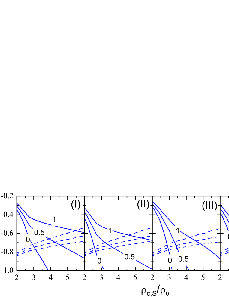
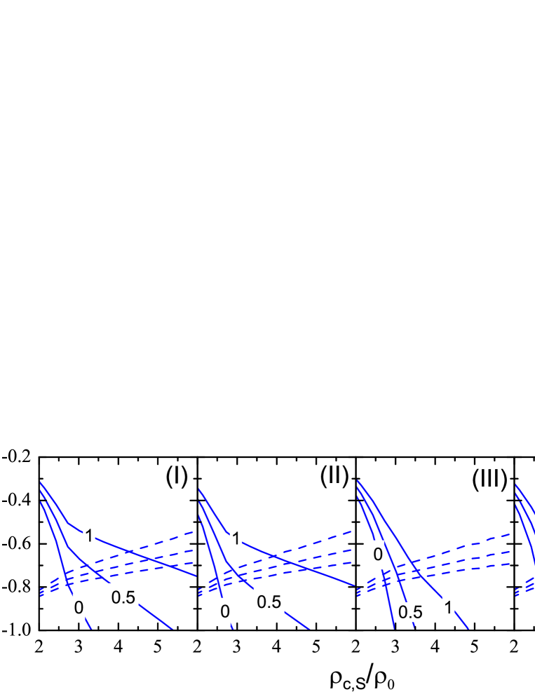
Figure 11: The quantities ${\alpha}_{\rm pole}(\mu_{e})$, $\omega_{\rm S}=\mu_{e}$, (solid lines) and $-1-\alpha_{\rm reg}$ (dash lines) are shown vs. critical density of a s-wave kaon condensation for various correlation parameter choices. Labels show values of $f^{\prime}_{\Lambda}=g^{\prime}_{\Sigma}$. Solid lines are drown for $f^{\prime}_{\Lambda\Sigma}=0$, and for $f^{\prime}_{\Lambda}=g^{\prime}_{\Sigma}=0,0.5,1$. Dashed lines are drown for three choices of the correlation parameters used in calculation of $\alpha_{\rm reg}$, $\xi_{nn}=\xi_{pp}=\xi_{np}=0,0.5,1$ (from the upper line to the lower one). Cases (I-IV) correspond to those in Fig. 1. In the upper plot the $\Sigma^{*}$ contributions are taken with $g^{\prime}_{\Sigma^{*}}=g_{\Sigma}$, $V_{\Sigma^{*}}=V_{\Sigma}$ and $g_{\sigma\Sigma^{*}}=g_{\sigma\Sigma}$. In the lower plot the $\Sigma^{*}$ is detached from the mean-field potentials $V_{\Sigma^{*}}=0$ and $g_{\sigma\Sigma^{*}}=0$. Hyperon populations are included in mean fields but not in the polarization operator.

In Figs. 11–12 we show values of $\alpha_{\rm pole}(\mu_{e})$ (solid lines) and $-1-\alpha_{\rm reg}$ (dash lines), calculated as a function of $\rho_{c,{\rm S}}$ for various baryon-baryon correlation parameters and for cases I–IV determining the hyperon couplings in (2). The $\Sigma$ hyperon contribution is proved to be very small and most part of the strength is due to the $\Lambda p^{-1}$ and $\Sigma^{*}n^{-1}$ contributions. Filling of the hyperon Fermi seas is not incorporated (we artificially suppress terms $\propto\Phi_{Hi}$ in $\Pi^{\rm pole}$). As we mentioned, embedding $\Sigma^{*}$ into the mean-field model (2) is quite uncertain due to the absence of any empirical constrain on the coupling constants. Therefore we consider two different cases. In the upper plot in Fig. 11 we assume that $\Sigma^{*}$ couples to the mean-field with the same strength as the $\Sigma$-hyperon ($V_{\Sigma^{*}}=V_{\Sigma}$, $g_{\sigma\Sigma^{*}}=g_{\sigma\Sigma}$), whereas in the lower plot in Fig. 11 we detach $\Sigma^{*}$ from the mean field potentials ($V_{\Sigma^{*}}=0$, $g_{\sigma\Sigma^{*}}=0$).

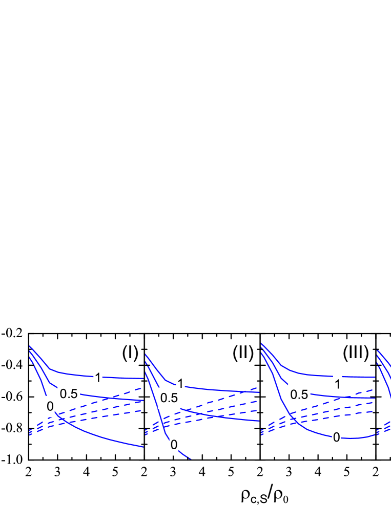
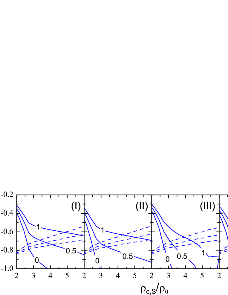
Figure 12: The same as in Fig. 11, but with account for the hyperon population in the polarization operator.

At the crossing point of the solid line with the corresponding dash line we have $\alpha_{\rm pole}=-1-\alpha_{\rm reg}$ and therefore $\alpha=0$, that means that given density is the critical density for both the s- and the p-wave condensations. When at the given value of $\rho_{\rm c,S}$ the solid line is below the corresponding dash line we have $\alpha_{\rm pole}<-1-\alpha_{\rm reg}$. This means that $\alpha<0$ and for such a parameter set $K^{-}$ condensation occurs in the p-wave state at somewhat smaller density than the assumed s-wave condensation.

The contributions from the hyperon Fermi seas are included in Figs. 12. From Figs. 11 and 12 we observe that $\Sigma^{*}$ contributes essentially to the $K^{-}$ polarization operator increasing attraction in the p-wave. The most favorable case for the p-wave condensation is realized if $\Sigma^{*}$ is detached from the mean field potentials. Comparing Figs. 11 and 12 we also see that the effects from the hyperon population on the $p$-wave terms are large.

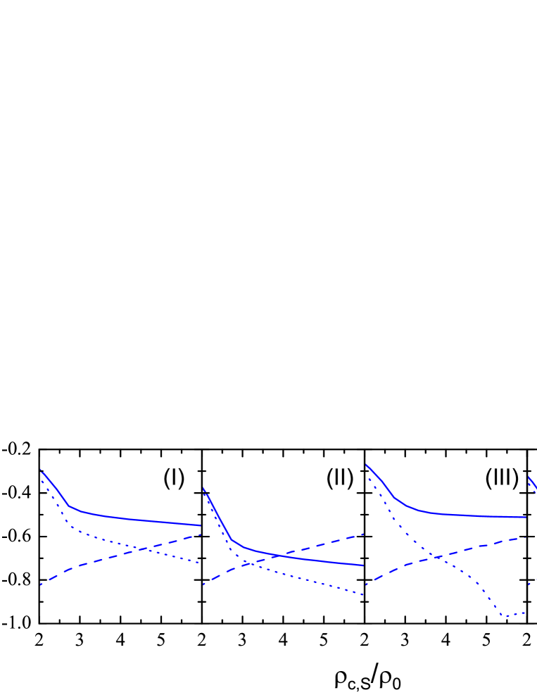
Figure 13: Values $\alpha_{\rm pole}$ (solid lines) and $-1-\alpha_{\rm reg}$ (dash lines), $\omega_{\rm S}=\mu_{e}$, calculated for the correlation parameters (79). Dotted lines present calculations with $\Sigma^{*}$ detached from mean field potentials. Planes correspond to the cases I-IV of hyperon couplings. Possibility of the hyperon population is also incorporated in the polarization operator.

In Fig. 13 we show the results of our calculations for the values of the correlation parameters, which we have evaluated in Sect. VII. For the $\Sigma^{*}$ detached from the mean-field potentials our model predicts a preference of the p-wave condensation. The p-wave condensation may occur already at $\rho\leq 3\rho_{0}$ for the cases II, IV, and for $\rho\simeq 4\rho_{0}$ and $\rho\simeq 4.5\rho_{0}$ for cases III and I provided the s-wave softening of the spectrum is also rather high. For $\Sigma^{*}$ coupled with the same strength as $\Sigma$ the s-wave condensation might be preferable compared to the p-wave condensation. Since a variation of other parameters, besides $\Sigma^{*}$ strength, is certainly also allowed the results are more uncertain in the latter case, cf. Figs  11 and 12.

VIII.3 I Order Phase Transition to the $K^{-}$ Condensate State

In the previous two sub-sections we have studied the possibility of the $K^{-}$ condensation assuming that it occurs by a second-order phase transition. Now we will investigate properties of $K^{-}$ excitations in the baryonic matter of different particle compositions, to figure out whether an abrupt ( of the first order) phase transition into a state with a new particle composition and another baryon density is energetically favorable.

We shall consider: (i) nucleon-hyperon matter (NHM) composition which we have discussed above, see Fig. 1; (ii) neutron-proton matter (NPM) composition, the matter consisting only of protons and neutrons assumed to be in $\beta$-equilibrium; (iii) isospin-symmetrical nuclear matter (ISM) composition consisting of protons and neutrons with $\rho_{p}=\rho_{n}$ and leptons, compensating the electric charge of the protons; and (iv) the proton-enriched matter (PEM) consisting of protons and neutrons with the concentration $Y_{p}=\rho_{p}/\rho=0.7$ and the charge compensated by the leptons. Thus in cases (ii)-(iv) we switch off the hyperons in our mean-field model (2) and in cases (iii), (iv) we also freeze the value of the proton concentration. For each case we shall calculate the total energy of the system with and without $K^{-}$ condensation. The idea behind this procedure is as follows. We consider the given configuration with the corresponding proton concentration and the condensate field as the most energetically favorable configuration until we did not prove the opposite. The full reaction balance is assumed to be recovered, thereby. Below we show that the first order phase transition occurs from NHM starting at the density $\rho^{\rm I}_{c}<\rho^{\rm II}_{c}$ to approximately ISM at $\rho^{\rm I}_{\rm fin}>\rho^{\rm I}_{c}$.

Figure 14: The energy of the lowest $K^{-}$ branch $\omega^{\rm min}(\boldsymbol{k}_{m},Y_{p},\rho)$ minimized in $|\boldsymbol{k}|$, and the electron chemical potential, calculated for the NHM, the NPM, ISM and PEM. In the right and left panels the results are presented with and without baryon-baryon correlation effects, respectively. In the NHM case interaction forces of case I are used and the $\Sigma^{*}$ contributions are taken with $g^{\prime}_{\Sigma^{*}}=g_{\Sigma}$, $V_{\Sigma^{*}}=V_{\Sigma}$ and $g_{\sigma\Sigma^{*}}=g_{\sigma\Sigma}$.

In Fig. 14 we show the energy of the lowest $K^{-}$ branch of the dispersion equation (80) $\omega^{\rm min}(\boldsymbol{k}_{m},Y_{p},\rho)$ minimized with respect to the momentum, as a function of the baryon density for different proton concentrations. We see that the more protons exist in the matter the smaller is the value of the density at which the minimal kaon energy $\omega^{\rm min}(\boldsymbol{k}_{m},Y_{p},\rho)$ meets the electron chemical potential. Therefore if the energy gain due to the condensation were large enough to compensate an energy loss in the fermion kinetic energies the system would undergo a first-order phase transition from the NHM state to the state with a proton enriched composition and a different density.

Let us first compare the energies of NHM, NPM, ISM and PEM taking into account a possibility of the $K^{-}$ condensation in each case. For densities, when $\omega^{\rm min}(\boldsymbol{k}_{m},Y_{p},\rho)>\mu_{e}$, there is no condensation and the energy density of the system is given by (4). When, at given $Y_{p}$ and $\rho$, we have $\omega^{\rm min}(\boldsymbol{k}_{m},Y_{p},\rho)<\mu_{e}$, the $K^{-}$ excitations appear, partially replacing the leptons. These excitations occupy single state and form a $K^{-}$ condensate. The electron chemical potential is fixed now as $\mu_{e}=\omega^{\rm min}(\boldsymbol{k}_{m},Y_{p},\rho)$. The energy density of the system with the $K^{-}$ condensate reads:

$$E_{\rm tot}^{(K)} = E_{\rm mes}+\sum_{B}E_{B}^{\rm kin}$$ (86)

$$+ \sum_{l=\mu\,e}E_{l}(\omega^{\rm min}(\boldsymbol{k}_{m},Y_{p},\rho))+E_{\rm cond}^{(K)}\,,$$

where $E_{\rm cond}^{(K)}$ is the energy density of the condensate field related to the mean field Lagrangian

$${\cal L}_{K} = \left(\omega^{2}-m^{2}_{K}-\boldsymbol{k}^{2}-\Pi(\omega,\boldsymbol{k})\right)|\phi_{\boldsymbol{k\,}}|^{2}.$$ (87)

The $\phi_{\boldsymbol{k}}$ is the $K^{-}$ condensate mean field with the wave vector $\boldsymbol{k}$. This field component should be found from the minimization of the appropriate thermodynamical potential. For simplicity we use here the linear model neglecting the higher order terms, as $\propto|\phi_{\boldsymbol{k\,}}|^{4}$, which incorporate an effective kaon-kaon interaction in dense baryonic matter. The effective kaon-kaon interaction depends on the structure of the mean field. In absence of the non-linear effective kaon-kaon interaction, within the variational procedure we obtain the field of the running plane wave type, $\phi_{\boldsymbol{k}}=\mbox{exp}(-i\omega^{\rm min}(\boldsymbol{k}_{m},Y_{p},\rho)t+i\boldsymbol{k}_{m}\boldsymbol{r})$. Using that the dispersion relation (80) is fulfilled for $\boldsymbol{k}=\boldsymbol{k}_{m}$ and $\omega=\omega^{\rm min}(\boldsymbol{k}_{m},Y_{p},\rho)$, and that the density of the charged kaon condensate $\rho_{K}$ is fixed by the electro-neutrality condition

$$\rho_{K}=\sum_{B}\,q_{B}\,\rho_{B}-\rho_{e}-\rho_{\mu^{-}}\,,$$

we find the energy density of the kaon condensate equal to

$$E_{\rm cond}^{(K)}=\omega^{\rm min}(\boldsymbol{k}_{m},Y_{p},\rho)\,\Big{(}\sum_{B}\,q_{B}\,\rho_{B}-\rho_{e}-\rho_{\mu^{-}}\Big{)}.$$

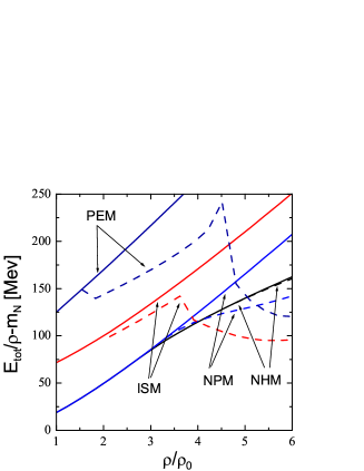
Figure 15: Total energy per baryon of the matter with different particle compositions: without a $K^{-}$ condensate (solid lines) and with the condensate (dashed lines). Abbreviations are the same, as in Fig. 14. The curves in the right and the left panels are drawn with and without inclusion of correlations. In the NHM case interaction forces of case I are used and the $\Sigma^{*}$ contributions are taken with $g^{\prime}_{\Sigma^{*}}=g_{\Sigma}$, $V_{\Sigma^{*}}=V_{\Sigma}$ and $g_{\sigma\Sigma^{*}}=g_{\sigma\Sigma}$.

In Fig. 15 we show the energy per baryon in the various baryonic systems, NHM, NPM, ISM, and PEM ($Y_{p}\simeq 0.7$), with and without the kaon condensate (dashed and solid lines, respectively). We see that for the density $\rho_{\rm c}\simeq 3\,\rho_{0}$ without baryon-baryon correlations and $\simeq 4\,\rho_{0}$ including correlations, the condensate state of ISM becomes to be energetically favorable compared to NHM. The transition to the new more symmetric isospin configuration would increase the Fermi energies of the leptons (the latter ones are needed to compensate a larger charge of protons), but reduce the symmetry energy of the nuclear matter and the total Fermi energy of nucleons. Without the $K^{-}$ condensate, the energy loss is larger than the gain and the system chooses the composition shown in Fig. 1 for the given EoS, cf. that in Fig. 14 the solid lines labeled ISM are lying above the NPM lines. With account for a possibility of the $K^{-}$ condensation one additionally gains on the kinetic energy of the leptons, which are replaced by kaons. The latter energy gain is large enough, leading to the preference of the ISM. The hyperon Fermi seas are not filled. It is more energetically preferable to create extra $K^{-}$ condensate mesons instead of a filling of a Fermi sea of the hyperons. From Fig. 15 we see that PEM ($Y_{p}\simeq 0.7$) has a larger energy than ISM. As it is also seen from Fig. 15 the resulting isospin composition can be only slightly above $Y_{p}=1/2$. Further on we neglect this difference considering ISM as the final configuration.

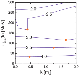
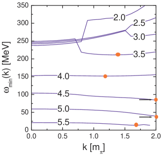
Figure 16: The energy of the lowest branch of the dispersion equation (80) as function of the momentum with the polarization operator (81) for the ISM at various densities (labels on the curves show the densities in $\rho_{0}$). Calculations, done without and with baryon-baryon correlations, are shown on left and right panels, respectively. Full circles mark the position of the minimum on the spectrum.

In Fig. 16 we plot the lowest branch of the $K^{-}$ excitation spectrum $\omega_{\rm min}(|\boldsymbol{k}|)$ in the ISM at various densities. In the left panel baryon-baryon correlations are switched off and in right panel, switched on. We see that for rather large densities ($\geq(2.5\div 3.5)\rho_{0}$) the spectra have minima (dots in Fig. 16) at finite values of the kaon momentum $\boldsymbol{k}_{m}\neq 0$. It signals that the transition from NHM to a dense ISM would occur as the first-order phase transition into the state with the p-wave kaon condensate. The calculations shown in Figs. 14-16 are done for $g^{\prime}_{\Sigma^{*}}=g_{\Sigma}$, $V_{\Sigma^{*}}=V_{\Sigma}$ and $g_{\sigma\Sigma^{*}}=g_{\sigma\Sigma}$. The results obtained with the $\Sigma^{*}$ detached from the mean field potentials are checked to be of minimal difference.

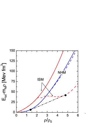
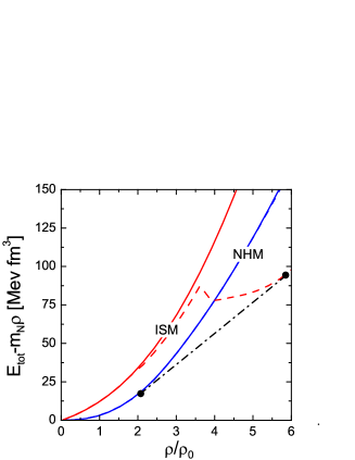
Figure 17: Energy densities of NHM and ISM with and without the $K^{-}$ condensate shown by dashed and solid lines, respectively. For NHM the forces of case I are used. Calculations with and without baryon-baryon correlations are shown in left and right panel respectively. The dash-dotted lines represent the double-tangent Maxwell constructions between two phases.

In the assumption that the surface tension is larger than a critical value the initial and final state densities are determined by the double-tangent Maxwell construction HPS93 ; VYT01 . In Fig. 17 we show the double-tangent construction between NHM and ISM states. We see that the critical density for the beginning of the first-order phase transition is equal to $\rho_{\rm c}^{\rm I}\simeq 1.4\rho_{0}$ without correlations and $\simeq 2.1\rho_{0}$ with correlations. The critical densities of the final state are $\rho_{\rm fin}^{\rm I}\simeq 5\rho_{0}$ and $\simeq 6\rho_{0}$, accordingly .

If surface tension is smaller than the critical value, the phase transition results in the mixed phase G92 ; HPS93 ; CGS00 ; VYT01 . Then the local charge-neutrality condition is relaxed being replaced to the global charge-neutrality condition. In this case the critical density for the appearance of the kaon condensate droplets within mixed phase is still smaller than that value given by the Maxwell construction. The presence of the mixed phase may have interesting observable consequences, see G01 and references therein.

Thus, relying on the analysis above, we argue that the actual critical density of the first-order phase transition can be even smaller than $2\rho_{0}$ and that this transition occurs into the p-wave condensate state.

IX Conclusion

In this work we constructed the $K^{-}$ polarization operator in dense baryonic matter of arbitrary isotopic composition, including both the s- and p-wave $K^{-}$-baryon interactions, and, using the relativistic mean field model to describe the baryon properties. We applied the derived polarization operator to the issue of the s- and p-wave $K^{-}$ condensations in neutron star interiors. We considered two different models of the equation of state, cf. Sect. II and Appendix A below. Finite temperature effects can be easily incorporated in our general scheme.

To describe the kaon - nucleon interaction we used the kaon-nucleon scattering amplitude obtained as a solution of the coupled-channel Bethe-Salpeter equation with the interaction kernel derived from the relativistic chiral SU(3) Lagrangian with the large $N_{c}$ constrains of QCD. We calculated explicitly the pole terms of the $K^{-}$ polarization operator related to $\Lambda p^{-1}$, $\Sigma N^{-1}$, $\Sigma^{*}N^{-1}$ excitations with $K^{-}$ quantum numbers and analyzed effects of the filling of the hyperon $H=(\Lambda,\Sigma,\Xi)$ Fermi seas at densities above the hyperonization point $\rho>\rho_{c,H}\simeq(2.5\div 3)\rho_{0}$.

In Fig. 6 we compared the s-wave regular part of our polarization operator with the simplified form, which is widely used in the literature. The $\Sigma$-term extracted from this comparison ($\Sigma\simeq 150$ MeV) is found to be two-three times smaller compared to that allows for the s-wave $K^{-}$ condensation in ordinary neutron star matter composed mostly of neutrons. However, we found the essential attractive support from the hyperon exchange terms of the p-wave scattering amplitude contributing to the s-wave part of the polarization operator, see (50). Inclusion of these terms, which were omitted in previous works, makes a second-order phase transition to the s-wave $K^{-}$ condensate state possible (at densities $\simeq 3\rho_{0}$ in given model, when the correlation effects are not included yet).

We evaluated baryon-baryon correlation parameters and corrected all the s- and p-wave terms of the polarization operator, accordingly. Inclusion of the correlations pushes the critical point of the second order phase transition to the s-wave $K^{-}$ condensate state up to larger densities ($\stackrel{{\scriptstyle\scriptstyle>}}{{\phantom{}{}_{\sim}}}(4\div 5)\rho_{0}$, cf. Figs. 10 and 20). We studied how much the results are sensitive to a variation of the correlation parameters. We estimated (see Appendix D) feed-back quantum fluctuation effects arguing that their contribution is not too large at the low kaon energies under consideration, and at zero temperature to the first approximation they can be neglected.

Our next observation (see Appendix D) is that at $\boldsymbol{k}=0$ the imaginary part of the pole term of the polarization operator is finite only in a rather narrow interval of kaon energies. Would the electron chemical potential cross the $K^{-}$ branch within this energy interval, the s-wave condensation would not occur. However this possibility is not realized for the parameter choice used in our model.

We checked the possibility of a second-order phase transition to the p-wave $K^{-}$ condensate state. We showed that, in the vicinity of the critical point of the s-wave $K^{-}$ condensation, the p-wave part of the polarization operator, induced mainly by $\Lambda$-proton holes and $\Sigma^{*}$-nucleon holes and some regular terms, is rather large and attractive. It may change the sign of the momentum derivative of the energy at the lowest $K^{-}$ spectrum branch at origin. If occurred, it would mean that we have p-wave condensate instead of the s-wave one at somewhat smaller density. We demonstrated that this statement, although being rather model dependent, holds for a wide range of varying parameters. The results essentially depend on the unknown value of the strength of the $\Sigma^{*}$ mean field potential. In most favorable case, when $\Sigma^{*}$ is detached from the mean field potentials, the second order phase transition to the p-wave condensate state may occur even at $\rho\sim 3\rho_{0}$ (with correlations included), cf. Fig. 13 and 21. This result is also sensitive to the details of the equation of state and the parameterization of the hyperon-nucleon interaction. For the equation of state with parameters (88) the critical density is increased compared to that one calculated with parameters (LABEL:lagconst).

We discussed the possibility of a first-order phase transition to a $K^{-}$ condensate state. We calculated the energies of the baryonic matter with different compositions with and without the inclusion of the $K^{-}$ condensation. We found that with account for a $K^{-}$ condensation, the isospin-symmetrical neutron-proton matter is more energetically favorable than the standard nucleon-hyperon-lepton matter at densities $\stackrel{{\scriptstyle\scriptstyle>}}{{\phantom{}{}_{\sim}}}3\div 4\rho_{0}$ (depending on the values of parameters of baryon-baryon correlations). The hyperon Fermi seas are melting at this phase transition. Hyperons are replaced by nucleons and electrons are replaced by the condensate $K^{-}$ mesons. We demonstrated that in dense isospin symmetrical $np$-matter the $K^{-}$ excitations are condensed in the p-wave state. With the help of the Maxwell construction we found that the critical density of the beginning of the phase transition is about $2\rho_{0}$ with the baryon-baryon correlations included, cf. Figs. 17 and 24. The final state density is about $(5\div 6)\rho_{0}$. Appearance of such a strong first order phase transition may have interesting observable consequences as blowing off a part of the exterior of the neutron star, a strong neutrino pulls, a gravitational wave, a strong pulsar glitch, etc. These consequences have been previously discussed in relation to the first order phase transition to the pion condensate state MSTV90 . Here we may expect a stronger energy release compared to the pion condensate phase transition since typical energy scale $m_{K}\gg m_{\pi}$.

Our derivations can be helpful not only for description of neutron star interiors, but also for discussion of kaonic effects in other nuclear systems, as atomic nuclei and heavy ion collisions. Therefore, of particular interest is the further more detailed analysis of the p-wave effects on $K^{-}$ spectra in nucleus-nucleus collisions motivated by present SIS and SPS experiments and the future SIS200 program.

In spite of a number of new effects was incorporated in our scheme, some other effects might be also important. Present calculations still suffer of many uncertainties, most of which are due to the lack of experimental information, e.g. on the coupling constants, the absence of unambiguous way for going off-mass shell and the lack of study of more complicated in-medium fluctuation effects, which we just roughly estimated in the present work. Among them, there are the pion softening effects MSTV90 , which can essentially affect the results at finite temperatures, and the contribution of the non-linear meson-meson interaction. The latter may partially suppress the condensate contribution to the energy beyond the critical point.

Diminishing of the uncertainties needs further theoretical and experimental work.

Appendix A Variation of the Parameters of the Baryon Interaction

In this section we investigate how much the results of Sec. VIII are sensitive to the particular choice of the EoS. For comparison with the results obtained within the relativistic mean-field model with the parameters (LABEL:lagconst) we use here the EoS in parameterization HH , which is a good fit to the optimal EoS of the Urbana–Argonne group Akmal up to a 4 times nuclear saturation density, smoothly incorporating the causality limit at higher densities.

The parameters of the mean-field model are adjusted to the following bulk parameters of the nuclear matter at saturation: $\rho_{0}=0.16$ fm^-3, binding energy $E_{\rm bind}=-15.8$ MeV, compression modulus $K=$250 MeV, symmetry energy $a_{\rm sym}=28$ MeV, and the effective nucleon mass $m_{N}^{*}(\rho_{0})=0.8\,m_{N}$. The corresponding coupling constants of the Lagrangian (2) are then as follows:

$$\frac{\displaystyle g_{\omega N}^{2}\,m_{N}^{2}}{\displaystyle m_{\omega}^{2}}=91.2506\,,\quad\frac{\displaystyle g_{\sigma N}^{2}\,m_{N}^{2}}{\displaystyle m_{\sigma}^{2}}=195.597\,,$$

$$\frac{\displaystyle g_{\rho N}^{2}\,m_{N}^{2}}{\displaystyle m_{\rho}^{2}}=77.4993\,,\quad b=0.0867497\,,$$

$$\quad c=0.0805981\,.$$ (88)

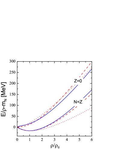
Figure 18: EoS for ISM ($N=Z$) and neutron ($Z=0$) matter calculated with the parameter set (LABEL:lagconst) (dotted lines) and with the parameter set (88) (dashed lines). The solid lines show the EoS from Ref. HH .

In Fig. 18 we show energies for the nucleon isospin-symmetrical matter (ISM) and the pure neutron matter for two choices of the mean-field EoS, the model (LABEL:lagconst), simulating a softer EoS and (88) simulating a stiffer Urbana-Argone EoS. In spite of the parameters (LABEL:lagconst) and (88) essentially deviate from each other, the energies and other thermodynamic characteristics of the neutron star matter are rather closed to each other in both the parameter choices in the absence of a $K^{-}$ condensate. For the ISM case the EoS with parameters (88) is significantly stiffer than the one calculated with parameters (LABEL:lagconst) at $\rho\stackrel{{\scriptstyle\scriptstyle>}}{{\phantom{}{}_{\sim}}}3\,\rho_{0}$.

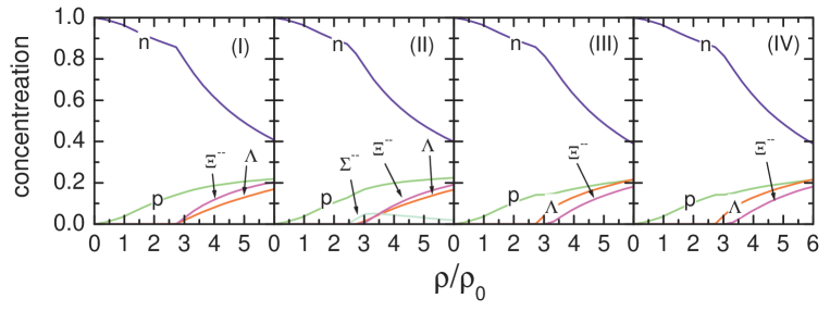
Figure 19: Concentration of baryon species in neutron star matter for EoS (88). Panels (I-IV) correspond to four choices of the hyperon-nucleon interaction parameters specified in text.

In Fig. 19 we show concentrations of the baryon species in neutron star matter corresponding to EoS given by the choice (88) for four choices of the hyperon-nucleon interaction (cases I - IV) which we are using in this paper. We see that the critical density of the hyperonization is approximately $3\rho_{0}$ for all the choices. General trends are the same as the ones shown by the corresponding curves discussed in the main text, see Fig. 1. The most essential difference is that the proton concentrations given by Fig. 19 are smaller than those in Fig. 1. This should have consequences for the neutrino cooling of the neutron star. Indeed, when the proton concentration enlarges $11\div 14\%$ the efficient cooling mechanism is switched on due to allowance of the direct Urca processes $p\rightarrow n+e+\bar{\nu}$. In principle, this difference may allow to select a more appropriate EoS in the future.

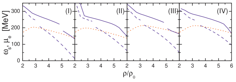
Figure 20: The same as in Fig. 10 but for the parameters (88).

Fig. 20 demonstrates the energy of the lowest $K^{-}$ branch of the dispersion equation (80) for $\boldsymbol{k}=0$ calculated with the mean field model with parameters (88). Dashed lines are computed without inclusion of correlations and solid lines, with inclusion of correlations. Comparing this figure with Fig. 10 presenting the same calculation but with the parameter choice (LABEL:lagconst) we see that the critical densities are increased for all the cases I-IV for the model (88). The second order phase transition to the s-wave $K^{-}$ condensate state occurs within the density interval $(3.5\div 6)\rho_{0}$ depending on the choice of the parameters. For the model (LABEL:lagconst) the corresponding interval of critical densities was $(3\div 5.5)\rho_{0}$.

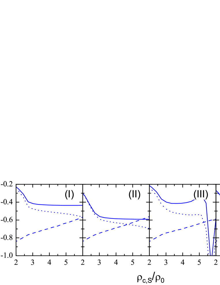
Figure 21: The same as in Fig. 13 but for the parameters (88).

In Fig. 21 we demonstrate the possibility of the second order phase transition to the p-wave state within the model with parameters (88) at the assumption that the system is in the vicinity of the critical point of the s-wave condensation. Solid curves relate to the model when $\Sigma^{*}$ is attached with the mean field potentials with the same strength as $\Sigma$ and dashed curves, when $\Sigma^{*}$ is detached from the mean field potentials. Comparing the curves with those curves presented in Fig. 13 for the parameter choice (LABEL:lagconst) we see that the general trends are the same in both cases. The second order phase transition to the p-wave state may occur in the model (88) for $\rho\geq(4.5\div 5.5)\rho_{0}$ in cases II - IV and it does not occur for case I up to $6\rho_{0}$.

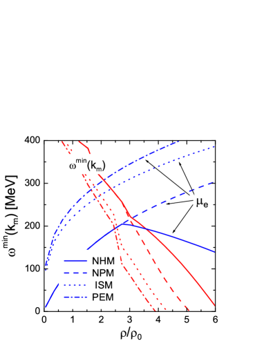
Figure 22: The same as in Fig. 14 but for the parameter set (88)

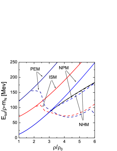
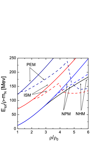
Figure 23: The same as in Fig. 15 but for the parameters (88).

Figs. 22, 23, 24 study the possibility of the first-order phase transition for the EoS with parameters (88). Again we see the same trends as given by corresponding Figs. 14, 15, 17. From Fig. 22 we see that the energy of the PEM crosses the electron chemical potential at a smaller density compared to ISM and NHM cases. Fig. 23 demonstrates that the energy of the ISM with the condensate (with correlations included) becomes to be lower than the energy of the NHM for $\rho\geq 4\rho_{0}$. This value ($4\rho_{0}$) is about the same as that for the EoS with parameters (LABEL:lagconst).

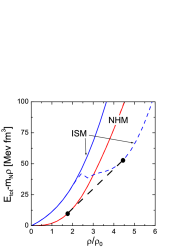
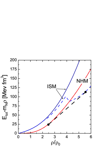
Figure 24: The same as in Fig. 17 but for the parameters (88).

In Fig. 24 we show the double-tangent construction for the EoS with parameters (88). The first order phase transition starts at the density $\rho^{\rm I}_{c}\simeq 2.5\rho_{0}$ (with correlations included). This value is only slightly larger than that ($2.1\rho_{0}$) given by the EoS with parameters (LABEL:lagconst). The final state density is $\rho^{\rm I}_{\rm fin}\simeq 5.5\rho_{0}$, i.e. slightly less than the value ($5.9\rho_{0}$) given by the model (LABEL:lagconst).

Thus the main conclusion, what we can do from the above comparison of the results obtained for two EoS with parameters (LABEL:lagconst) and (88), is that all the general trends in the behavior of the kaon condensation are the same. The critical densities of the s- and p-wave condensations are only slightly higher in the framework of the model with parameters (88).

Appendix B Non-Equilibrium Green’s functions

Two-point (2P) functions (a Green’s function or a self-energy) are introduced within the Schwinger-Baym-Kadanoff-Keldysh approach as, cf. IKV00 ,

$$iF(x,y)=\left(\begin{array}[]{ccc}iF^{--}(x,y)&&iF^{-+}(x,y)\\[8.53581pt] iF^{+-}(x,y)&&iF^{++}(x,y)\end{array}\right)$$ (91)

$$=\left(\begin{array}[]{ccc}\left<{\cal T}\widehat{A}(x)\widehat{B}(y)\right>&&\mp\left<\widehat{B}(y)\widehat{A}(x)\right>\\[14.22636pt] \left<\widehat{A}(x)\widehat{B}(y)\right>&&\left<{\cal T}^{-1}\widehat{A}(x)\widehat{B}(y)\right>\end{array}\right),$$ (94)

where ${\cal T}$ and ${\cal T}^{-1}$ are the usual time and anti-time ordering operators. Note that, compared to Green’s functions, “$\pm\,\mp$” self-energies would have extra sign $-$ since they include vertices $V^{-}=-iV_{0}$ and $V^{+}=+iV_{0}$.

Not all four components of $F$ are independent. The following relations between non-equilibrium and usual retarded and advanced functions are fulfilled

$$F^{R}(x,y) = F^{--}(x,y)-F^{-+}(x,y)$$

$$= F^{+-}(x,y)-F^{++}(x,y)$$

$$:= \theta(x_{0}-y_{0})\left(F^{+-}(x,y)-F^{-+}(x,y)\right),$$

$$F^{A}(x,y) = F^{--}(x,y)-F^{+-}(x,y)$$ (95)

$$= F^{-+}(x,y)-F^{++}(x,y)$$

$$:= \theta(y_{0}-x_{0})\left(F^{-+}(x,y)-F^{+-}(x,y)\right),$$

where $\theta(x_{0}-y_{0})$ is the step function of the time difference. For such 2P-functions complex conjugation implies

$$\left(iF^{-+}(x,y)\right)^{\rm C} = iF^{-+}(y,x)\quad\Rightarrow\quad iF^{-+}(X,p)=\mbox{real},$$

$$\left(iF^{+-}(x,y)\right)^{\rm C} = iF^{+-}(y,x)\quad\Rightarrow\quad iF^{+-}(X,p)=\mbox{real},$$

$$\left(iF^{--}(x,y)\right)^{\rm C} = iF^{++}(y,x)$$

$$\Rightarrow \quad\left(iF^{--}(X,p)\right)^{*}=iF^{++}(X,p),$$

$$\left(F^{R}(x,y)\right)^{\rm C} = F^{A}(y,x)$$

$$\Rightarrow \quad\left(F^{R}(X,p)\right)^{*}=F^{A}(X,p),$$ (96)

where the right parts specify the properties of the 2P-functions in the Wigner representation,

$$F(X,p)=\intop\frac{{\rm d}^{4}\xi}{(2\pi)^{4}}\,e^{-i\,(p\cdot\xi)}F(X+\xi,X-\xi)$$ (97)

with $X=\frac{1}{2}(x+y)$ and $p=(\epsilon,\boldsymbol{p}\,)$. The conjugation operation is defined as a $\big{(}\dots\big{)}^{\rm C}=\big{(}\dots\big{)}^{*}$ for bosons and $\big{(}\dots\big{)}^{\rm C}=\gamma_{0}\,\big{(}\dots\big{)}^{\dagger}\,\gamma_{0}$ for fermions.

We denote the fermionic Green’s function and self-energy as $\widehat{G}^{a,b}$ and $\widehat{\Sigma}^{a,b}$, respectively, and the bosonic ones as $D^{a,b}$ and $\Pi^{a,b}$. The hats on the fermionic 2P-functions point on their spin structure, e.g., $\widehat{G}^{R,A}=[p\!\!\!/-m_{\rm f}-\widehat{\Sigma}^{R,A}(p)]^{-1}$.

For systems in equilibrium, the “$-+$” Green’s functions, the spectral functions and occupation numbers are related by the Kubo-Schwinger-Martin condition:

$$i\widehat{G}^{-+}(p)=-\widehat{A}_{\rm f}(p)\,n^{\rm f}(\epsilon)\,,\,$$

$$i\widehat{G}^{+-}(p)=\widehat{A}_{\rm f}(p)\,[1-n^{\rm f}(\epsilon)]\,,$$

$$iD^{-+}(p)=A_{\rm b}(p)\,n^{\rm b}(\epsilon)\,,\,$$

$$iD^{+-}(p)=A_{\rm b}(p)\,[1+n^{\rm b}(\epsilon)]\,,$$ (98)

$$i\widehat{\Sigma}^{-+}(p)=\widehat{\gamma}_{\rm f}(p)\,n^{\rm f}(\epsilon)\,,\,$$

$$i\widehat{\Sigma}^{+-}(p)=-\widehat{\gamma}_{\rm f}(p)\,[1-n^{\rm f}(\epsilon)]\,,$$

$$i\Pi^{-+}(p)=-\gamma_{\rm b}(p)\,n^{\rm b}(\epsilon)\,,\,$$

$$i\Pi^{+-}(p)=-\gamma_{\rm b}(p)\,[1+n^{\rm b}(\epsilon)]\,,$$ (99)

where $\widehat{A}_{\rm f}(p)=-2{\rm Im\,}\widehat{G}^{R}_{\rm f}(p)$, $A_{\rm b}(p)=-2{\rm Im\,}D^{R}_{\rm b}(p)$ are the fermion and the boson spectral functions, $\widehat{\gamma}_{\rm f}(p)=-2{\rm Im\,}\widehat{\Sigma}^{R}_{\rm f}(p)$, $\gamma_{\rm b}=-2{\rm Im\,}\Pi^{R}_{\rm b}$ are the corresponding widths, and

$$n^{{\rm f,b}}(\epsilon)=\{\exp[(\epsilon-\mu_{{\rm f,b}}/T]\pm 1\}^{-1}$$ (100)

are fermion/boson occupation numbers, with $\mu_{\rm f,b}$ standing for the fermionic and bosonic chemical potentials.

In the quasiparticle approximation ($\gamma_{\rm b}\rightarrow 0$ in the bosonic Green’s functions) we have for bosons

$$A_{\rm b}(q) \approx 2\pi\delta[q_{0}^{2}-\boldsymbol{q}^{2}-m_{\rm b}^{2}-{\rm Re\,}\Pi^{R}(q_{0},\boldsymbol{q}\,)]$$

$$= \sum_{i}2\pi Z_{\boldsymbol{q}}^{{\rm b},i}\delta(q_{0}-\omega_{\rm b}^{i}({\boldsymbol{q}}))\,,$$

$${\rm Re\,}D_{\rm b}^{R}(q) \approx \sum_{i}\frac{Z_{\boldsymbol{q}}^{{\rm b},i}}{q_{0}-\omega_{\rm b}^{i}({\boldsymbol{q}})},$$ (101)

where $Z_{\boldsymbol{q}}^{{\rm b},i}=1/[2q_{0}-\partial\mbox{Re}\Pi^{R}/\partial q_{0}]_{q_{0}=\omega_{\rm b}^{i}(\boldsymbol{q})}$ are quasiparticle normalization corresponding to the given spectrum branch $\omega_{\rm b}^{i}(\boldsymbol{q}\,)$.

As a step to a non-relativistic limit it is convenient to approximate the spin structure of the fermionic Green’s functions as $\widehat{G}_{\rm f}^{R}(p)=(p\!\!\!/+m_{\rm f})\,G_{\rm f}^{R}(p)$ and $\widehat{A}_{\rm f}(p)=(p\!\!\!/+m_{\rm f})\,A_{\rm f}(p)$. In the quasiparticle approximation ($\gamma_{\rm f}\rightarrow 0$) we have

$$A_{\rm f}(p) \approx 2\pi\delta[\epsilon^{2}-\epsilon^{2}_{0}(\boldsymbol{p})-{\rm Re\,}\Sigma^{R}(\epsilon,\boldsymbol{p})]$$

$$= Z_{\boldsymbol{p}}^{\rm f}\,\frac{\pi}{\epsilon_{\boldsymbol{p}}}\,\delta(\epsilon-\epsilon_{\boldsymbol{p}}),\,$$

$${\rm Re\,}G_{\rm f}^{R}(\epsilon,\boldsymbol{p}\,) \approx \frac{1}{2\,\epsilon_{\boldsymbol{p}}}\,\frac{Z_{\boldsymbol{p}}^{\rm f}}{\epsilon-\epsilon_{\boldsymbol{p}}}$$

$$Z_{\boldsymbol{p}}^{\rm f} = \left[1-\partial{\rm Re\,}\Sigma^{R}/\partial\epsilon^{2}\Big{|}_{\epsilon=\epsilon_{\boldsymbol{p}}}\right]^{-1},$$ (102)

where $\epsilon_{\boldsymbol{p}}$ obeys the dispersion equation $\epsilon_{\boldsymbol{p}}^{2}=\epsilon^{2}_{0}(\boldsymbol{p})+{\rm Re\,}\Sigma^{R}(\epsilon_{\boldsymbol{p}},\boldsymbol{p})$ with $\epsilon_{0}(\boldsymbol{p})=\sqrt{m_{\rm f}^{2}+\boldsymbol{p}^{\,2}}$. The self-energy $\Sigma^{R}$ includes averaging over the spin structure, $\Sigma^{R}=\frac{1}{2}\,{\rm Tr}\{\widehat{\Sigma}^{R}\cdot(p\!\!\!/+m_{\rm f})\}$

The mean-field solutions (3) of the equation of motion for a baryon $B$, following from (2), can be parameterized by the self-energy $\Sigma^{R}(\epsilon,\boldsymbol{p}\,)=2\,V_{B}\,\epsilon+V_{B}^{2}-2\,m_{N}\,g_{\sigma}\,\sigma+g_{\sigma B}^{2}\,\sigma^{2}$. Then we have $\epsilon_{\boldsymbol{p}}=E_{B}(\boldsymbol{p}\,)$, with $E_{B}(\boldsymbol{p}\,)$ defined in (3) and $Z_{\boldsymbol{p}}^{B}=[1-V_{B}/E_{B}(\boldsymbol{p}\,)]^{-1}=1+V_{B}/\epsilon_{B}(\boldsymbol{p}\,)\approx 1$.

The in-medium distributions of particles of given species over the momenta are

$$\frac{{\rm d}^{3}N_{\rm b}}{{\rm d}^{3}X{\rm d}^{3}k/(2\pi)^{3}} = \int_{0}^{\infty}\frac{{\rm d}\epsilon}{2\pi}2\epsilon A_{\rm b}(n^{\rm b}_{\epsilon}+1/2),$$ (103)

$$\frac{{\rm d}^{3}N_{\rm f}}{{\rm d}^{3}X{\rm d}^{3}k/(2\pi)^{3}} = \int_{0}^{\infty}\frac{{\rm d}\epsilon}{2\pi}A_{\rm f}(n^{\rm f}_{\epsilon}-1/2).$$ (104)

The terms $\mp 1/2$ are due to quantum fluctuations and should be properly renormalized with the corresponding subtraction of the vacuum pieces. The contributions corresponding to the integration over the negative energies are to be included in the distribution of antiparticles.

Appendix C Imaginary part of the Lindhard’s function

The imaginary part of the Lindhard’s function (28) is determined by the integral

$${\rm Im\,}\Phi_{iH}(\omega,\boldsymbol{k}) = -\frac{m_{N}^{*}}{2\,\pi\,|\boldsymbol{k}|}\intop_{m_{N}^{*}}^{\epsilon_{i}(p_{{\rm F}i})}{\rm d}E\,\theta\Big{[}4\,\boldsymbol{k}^{2}\,(E^{2}-m_{N}^{*\,2})$$

$$- (2\,\omega\,E+\omega^{2}-\boldsymbol{k}^{2}+m_{N}^{*\,2}-m_{H}^{*\,2})^{2}\Big{]}\,.$$

For brevity of notations we omitted here the vector potentials of baryons which can be recovered at the very end by the gauge invariant substitution $\omega\to\omega+v_{iH}$. The area where the imaginary part is finite is determined by the inequality

$$4\,\boldsymbol{k}^{2}\,(E^{2}-m_{N}^{*\,2})-(2\,\omega\,E+\omega^{2}-\boldsymbol{k}^{2}+m_{N}^{*\,2}-m_{H}^{*\,2})^{2}>0,$$

which has solutions $E>E^{+}_{iH}(\omega,\boldsymbol{k})$ and $E<E^{-}_{iH}(\omega,\boldsymbol{k})$ for $\omega^{2}<\boldsymbol{k}^{2}$, and $E^{-}_{iH}(\omega,\boldsymbol{k})<E<E^{+}_{iH}(\omega,\boldsymbol{k})$ for $\omega^{2}<(m_{\Lambda}^{*}-m_{N}^{*})^{2}$ and $\omega^{2}>(m_{\Lambda}^{*}+m_{N}^{*})^{2}+\boldsymbol{k}^{2}$ with

$$E_{iH}^{\pm}(\omega,\boldsymbol{k})=\frac{\,\left(-\omega\,\bar{E}(k^{2},m_{N}^{*\,2},m_{H}^{*\,2})\pm|\boldsymbol{k}|\,Q(k^{2},m_{N}^{*\,2},m_{H}^{*\,2})\right)}{\sqrt{\omega^{2}-\boldsymbol{k}^{2}}}\,.$$

One can check that $E_{iH}^{-}(\omega,\boldsymbol{k})<m_{N}^{*}$, if $\omega^{2}<\boldsymbol{k}^{2}$, and $E_{iH}^{-}(\omega,\boldsymbol{k})>m_{N}^{*}$, if $\omega^{2}>\boldsymbol{k}^{2}$. Therefore, in the case $\omega^{2}<\boldsymbol{k}^{2}$ we obtain

$${\rm Im\,}\Phi_{iH}^{(1)}(\omega,\boldsymbol{k}) = -\frac{m_{N}^{*\,2}}{2\,\pi\,|\boldsymbol{k}|}\,\Big{(}\epsilon_{i}(p_{{\rm F}i})-E_{iH}^{+}(\omega,\boldsymbol{k})\Big{)}$$

$$\times \theta\Big{(}\epsilon_{i}(p_{{\rm F}i})-E_{iH}^{+}(\omega,\boldsymbol{k})\Big{)}.$$

The condition $\epsilon_{i}(p_{{\rm F}i})>E_{iH}^{+}(\omega,\boldsymbol{k})$ imposes the following restriction on the frequency:

$$\epsilon_{H}(p_{{\rm F}i}-|\boldsymbol{k}|)<\omega+\epsilon_{i}(p_{{\rm F}i})<\epsilon_{H}(p_{{\rm F}i}+|\boldsymbol{k}|)\,.$$ (105)

In the other case $\boldsymbol{k}^{2}<\omega^{2}<(m_{H}^{*}-m_{N}^{*})^{2}+\boldsymbol{k}^{2}$ we find

$${\rm Im\,}\Phi_{iH}^{(2)}(\omega,\boldsymbol{k})=-\theta\Big{(}\epsilon_{i}(p_{{\rm F}i})-E_{iH}^{-}(\omega,\boldsymbol{k})\Big{)}$$

$$\times\frac{m_{N}^{*\,2}}{2\,\pi\,|\boldsymbol{k}|}\,\Big{(}\min\{\epsilon_{i}(p_{{\rm F}i}),E_{iH}^{+}(\omega,\boldsymbol{k})\}-E_{iH}^{-}(\omega,\boldsymbol{k})\Big{)}.$$

For $\boldsymbol{k}^{2}<\omega^{2}$ the condition $\epsilon_{i}(p_{{\rm F}i})<E_{iH}^{-}(\omega,\boldsymbol{k})$ puts the same restriction on frequency, as (105). Within this interval we always have $\epsilon_{i}(p_{{\rm F}i})>E_{iH}^{+}(\omega,\boldsymbol{k})$ and hence

$${\rm Im\,}\Phi_{iH}^{(2)}(\omega,\boldsymbol{k}) = -\frac{m_{N}^{*\,2}}{\pi}\,\frac{Q(k^{2},m_{N}^{*\,2},m_{H}^{*\,2})}{\sqrt{\omega^{2}-\boldsymbol{k}^{2}}}$$

$$\times \theta\Big{(}\epsilon_{i}(p_{{\rm F}i})-E_{iH}^{-}(\omega,\boldsymbol{k})\Big{)}.$$

Appendix D Evaluation of Fluctuation Terms

Let us discuss corrections to the kaon polarization operator which we did not take into account yet. We mean the fluctuation terms, which describe changes of the baryon propagation due to radiation and capture of virtual mesons, analogous to the Lamb shift in QED. Calculating the corresponding diagrams we shall use the Schwinger-Baym-Kadanoff-Keldysh (SBKK) technique, albeit, for systems at equilibrium and zero temperature the standard Feynman technique is equally appropriate. In the SBKK technique together with usual causal Green’s functions $G^{--}$ there appear time-disordered objects $G^{-+}$ and $G^{+-}$ which have meaning of Wigner’s densities, cf. (94). In general non-equilibrium case these Wigner’s densities obey the generalized kinetic equation IKV00 , being therefore very convenient for description of the fluctuative effects. Some relations between non-equilibrium Green’s functions were introduced in Appendix B. We will estimate fluctuation effects to the baryon self-energies and feedback from the kaon modification in medium to the polarization operator.

D.1 Correction of the Baryon Green’s Functions Due to Kaon Fluctuations

In Refs. LF01 ; Oset ; smed ; RO00 ; ske ; KL01 it was argued that the fluctuation contributions to the hyperon self-energy are essential at low densities and at the kaon energies not far away from the mass-shell. This is, particularly, due to the presence of the dynamically generated $\Lambda(1405)$ resonance close the kaon-nucleon threshold. This resonance dominates the s-wave kaon polarization operator at $\omega\sim m_{K}$ and is very sensitive to the Pauli-blocking effect and to the modification of the kaon spectral density. At lower kaon frequencies, typical in our case, the influence of the $\Lambda(1405)$ resonance is small. Thus, there remains to analyze the self-energy contributions of $\Lambda(1116)$, $\Sigma(1195)$ and $\Sigma^{*}(1385)$ resonances. Here we will demonstrate that in the low energy region and at the proton-neutron densities of our interest these contributions are rather suppressed.

Let us first show this on example of the diagram

$$\Sigma=\parbox{85.35826pt}{\includegraphics[clip={true},width=85.35826pt]{hse-kn-E.eps}}\,\,\,.$$ (106)

This is the self-energy insertion to the full hyperon Green’s function due to the $KN$ intermediate states. In (106) we draw full vertices and the nucleon line represents the full Green’s function. To be specific let us concentrate on the kaon-proton self-energy insertion for the $\Lambda$ hyperon. This corresponds to $H=\Lambda$, $K=K^{+}$ (according to selected arrow direction), $N=p$ in the diagram (106).

Within the SBKK diagram technique, using relations (B) between the retarded and “$-,+$” Green’s functions and self-energies we obtain, cf. KV96 ,

$$-i\widehat{\Sigma}^{R}(p) = \int\widehat{V}\left[\widehat{G}^{-+}(p+q)D^{R}(q)\right.$$ (107)

$$+ \widehat{G}^{R}(p+q)D^{-+}(q)-i\widehat{G}^{-+}(p+q)2{\rm Im\,}D^{R}(q)$$

$$+ \left.\widehat{G}^{R}(p+q)\,D^{R}(q)\right]\,\widehat{V}\frac{{\rm d}^{4}q}{(2\pi)^{4}}.$$

Here $-i\widehat{V}=-i\widehat{V}_{0}\,\Gamma$ and $-i\widehat{V}_{0}$ are the full and bare “$-$” vertices, and $i\widehat{V}=i\widehat{V}_{0}\,\Gamma$, $i\widehat{V}_{0}$ are the corresponding “$+$” vertices, $\Gamma$ is a scalar form-factor, which includes short-range nucleon-baryon correlations and simulates, thereby, the difference between the bare and the full vertices.

The last term in (107) vanishes identically, since the both retarded Green’s functions have the pole in the same complex $q_{0}$-semi-plane.

To separate the contributions from particles $K^{+}$ and antiparticles $K^{-}$, we may use the following decompositions of the retarded Green’s functions and the Wigner’s densities

$$D^{R}(q) = \theta(q_{0})D^{R}_{K^{+}}(q)+\theta(-q_{0})D^{A}_{K^{-}}(-q)\,,$$ (108)

$$D^{-+}(q) = \theta(q_{0})D^{-+}_{K^{+}}(q)+\theta(-q_{0})D^{+-}_{K^{-}}(-q)\,.$$ (109)

This allows to reduce integration over $q_{0}$ in (107) to the positive values. for $\Lambda$ self-energy we have

$$\Sigma^{R}(p) = \frac{1}{2}\,{\rm Tr}\{\widehat{\Sigma}^{R}\,(p\!\!\!/+m_{\Lambda}^{*})\}=\int\frac{{\rm d}^{4}q\,\theta(q_{0})}{(2\pi)^{4}}\,2\,m_{\Lambda}^{*}\,\overline{V^{2}}$$ (110)

$$\times \Big{\{}iG^{-+}(p+q)\,[D^{R}_{K^{+}}(q)-2\,i\,{\rm Im\,}D_{K^{+}}^{R}(q)]$$

$$\quad+G^{R}(p+q)\,iD^{-+}_{K^{+}}(q)$$

$$\quad+iG^{-+}(p-q)\,[D^{R}_{K^{-}}(q)-2\,i\,{\rm Im\,}D_{K^{-}}^{R}(q)]$$

$$\quad+G^{R}(p-q)\,iD^{-+}_{K^{-}}(q)\Big{\}}\,,$$

where we used notation

$$\overline{V^{2}} = \overline{V_{0}}^{2}\,\Gamma^{2}(q)\,,\quad$$

$$\overline{V_{0}^{2}} = C^{2}_{KN\Lambda}\,$$ (111)

$$\times \frac{1}{2}{\rm Tr}\Big{\{}\frac{(p\!\!\!/+m^{*}_{\Lambda})}{2\,m^{*}_{\Lambda}}\,q\!\!\!/\gamma_{5}\,\frac{(p\!\!\!/-q\!\!\!/+m^{*}_{N})}{2m^{*}_{N}}\,q\!\!\!/\gamma_{5}\Big{\}}.$$

Having in mind that we are interested in the self-energy insertion to the $\Lambda-p^{-1}$ loop, expanding denominators of the fermionic Green’s functions near the poles, and assuming that fermions are nonrelativistic, we may put $(p\cdot q)\simeq m_{N}^{*}\omega$, $p^{2}\simeq m_{N}^{*2}$ and $\omega,|\boldsymbol{q}|,(m_{\Lambda}^{*}-m_{N}^{*})\ll m_{\Lambda}^{*},m_{N}^{*}$. Then we come to the non-relativistic p-wave vertex $\overline{V^{2}_{0}}\simeq v_{0}^{2}\boldsymbol{q}^{\,2}$, with $v_{0}^{2}=C_{KN\Lambda}^{2}\,m_{N}^{*}/m_{\Lambda}^{*}\simeq(0.3\div 0.5)/m_{\pi}^{2}$. For $\Sigma$ hyperon we would have $v_{0}^{2}=C_{KN\Sigma}^{2}\,m_{N}^{*}/m_{\Sigma}^{*}\simeq(0.07\div 0.09)/m_{\pi}^{2}$, and for $\Sigma^{*}$ the corresponding coupling is $v_{0}^{2}=\frac{2}{3}\,C_{KN\Sigma^{*}}^{2}\,m_{N}^{*}/m_{\Sigma^{*}}^{*}\simeq(0.3\div 0.5)/m_{\pi}^{2}$.

To evaluate $\mbox{Im}\Sigma^{R}$ and $\mbox{Re}\Sigma^{R}$ we use the quasiparticle approximation for the spectral functions (B). As we shall see below non-quasiparticle corrections to the intermediate fermion Green’s functions, although exist, produec small contributions to the self-energies at kaon energies of interest.

We first evaluate ${\rm Im\,}\Sigma^{R}$. Using (98), (B), (B) we get from (107)

$$\frac{{\rm Im\,}\Sigma^{R}(\epsilon,\boldsymbol{p})}{2m_{\Lambda}^{*}}=-\sum_{i}\frac{1}{2}\int\frac{{\rm d}^{3}q}{(2\pi)^{2}}\,v_{0}^{2}\boldsymbol{q}^{\,2}\Gamma^{2}$$

$$\times\Big{\{}Z_{\boldsymbol{q}}^{K^{-},i}\,[1-n^{p}_{\boldsymbol{p}-\boldsymbol{q}}]\,\delta(\Delta^{i}_{-}(\epsilon,\boldsymbol{p},\boldsymbol{q}\,))$$

$$+Z_{\boldsymbol{q}}^{K^{+},i}n^{p}_{\boldsymbol{p}+\boldsymbol{q}}\,\delta(\Delta^{i}_{+}(\epsilon,\boldsymbol{p},\boldsymbol{q}))\Big{\}},$$

$$\Delta^{i}_{\pm}(\epsilon,\boldsymbol{p},\boldsymbol{q}\,)=\epsilon\pm\omega_{K^{\pm}}^{i}(\boldsymbol{q})-E_{p}(\boldsymbol{p}\pm\boldsymbol{q}),$$ (112)

where $i$ runs over all the $K^{-}$ and $K^{+}$ branches. Here $\omega_{K}^{i}(\boldsymbol{q})$ are functions of $\boldsymbol{q}^{\,2}$, and $n_{\boldsymbol{p}}^{p}=\theta(p_{{\rm F},p}-|\boldsymbol{p}\,|)$ is the proton occupation function. Following Appendix B we put $Z_{\rm f}=1$. We used also that occupations of real $K^{+}$ and $K^{-}$ mesons are absent at $T=0$ (we do not consider here the processes on the kaon condensate field).

As it is seen from the $\delta$ functions in (D.1), in the interesting for us region $\omega_{K^{-}}\stackrel{{\scriptstyle\scriptstyle<}}{{\phantom{}{}_{\sim}}}E_{\Lambda}(0)-E_{p}(0)$ there is only the contribution of the lowest $K^{-}$ spectrum branch.

Further evaluation is easily done taking $\boldsymbol{p}=0$, for simplicity. Thus, we obtain that for positive $\epsilon$ the imaginary part differs from zero only for $\epsilon>\omega_{K^{-}}(0)+E_{p}(0)$ and is equal to

$$\frac{{\rm Im\,}\Sigma^{R}(\epsilon,0)}{2\,m_{\Lambda}^{*}}=-\frac{v_{0}^{2}}{4\pi\,\alpha}\,Z_{\bar{q}}^{K^{-}}\,\Gamma^{2}(\bar{q})\,\bar{q}^{3}\theta(\bar{q}-p_{{\rm F},p})\,,$$ (113)

where $\bar{q}$ is a solution of the equation $\Delta_{-}(\epsilon,0,\bar{q})=0$ and $\alpha=-\partial\Delta_{-}(\epsilon,0,\boldsymbol{q}\,)/\partial\boldsymbol{q}^{\,\,2}|_{\boldsymbol{q}^{2}=\bar{q}^{2}}>0$. If $\bar{q}$ is small, namely, $-\Delta_{-}(\epsilon,0,0)\,\frac{\partial\Delta_{-}(\epsilon,0,q)}{\partial\boldsymbol{q}^{2}}\Big{|}_{\boldsymbol{q}^{2}=0}\ll 1$, we may approximate $\bar{q}\approx\bar{q}_{0}=\sqrt{\Delta_{-}(\epsilon,0,0)/\alpha_{0}}$, where $\alpha_{0}=-\frac{\partial\Delta_{-}(\epsilon,0,q)}{\partial\boldsymbol{q}^{2}}\Big{|}_{\boldsymbol{q}^{2}=0}$ . As it follows from the $\theta$ function in (113), fluctuations contribute to the imaginary part of the given diagram only, if $\epsilon>\omega_{K^{-}}(0)+E_{p}(0)+p_{{\rm F},p}^{2}\alpha_{0}$.

From Fig. 16 we see that $\omega_{K^{-}}(\boldsymbol{q})$ is very flat function of $\boldsymbol{q}^{2}$, and we can, therefore, neglect the momentum dependence of the $K^{-}$ spectrum for $0<|\boldsymbol{q}|\stackrel{{\scriptstyle\scriptstyle<}}{{\phantom{}{}_{\sim}}}2~{}m_{\pi}$. Then we can estimate the imaginary part of the diagram at finite $\boldsymbol{p}$ as follows

$$\frac{{\rm Im\,}\Sigma^{R}(\epsilon,\boldsymbol{p})}{2\,m_{\Lambda}^{*}}=-v_{0}^{2}\!\!\intop_{||\boldsymbol{p}\,|-\bar{q}_{0}|}^{|\boldsymbol{p}\,|+\bar{q}_{0}}\!\!\frac{{\rm d}|\boldsymbol{q}|\,|\boldsymbol{q}|^{3}}{8\pi\,|\boldsymbol{p}|}\,Z_{\boldsymbol{q}}^{K^{-}}\,\Gamma^{2}\,$$

$$\times 2\,[m_{N}^{*}+\Delta_{-}(\epsilon,0,0)]\,\theta[\Delta(\epsilon,p_{{\rm F},p},0)]$$

$$\approx-\frac{v_{0}^{2}\,m_{N}^{*}}{2\pi}\,Z_{\bar{q}_{0}}^{K^{-}}\,\Gamma^{2}(\bar{q}_{0})\,\bar{q}_{0}\,(\bar{q}_{0}^{2}+\boldsymbol{p}^{2})\,\theta[\Delta(\epsilon,p_{{\rm F},p},0)]\,.$$

(114)

The energy and momentum of the $\Lambda$ within the $\Lambda p^{-1}$ loop contributing to the $K^{-}$ polarization operator at the zero external momentum $\boldsymbol{q}$ are $\epsilon=E_{p}(\boldsymbol{p})+\omega_{K^{-}}(0)$ with $|\boldsymbol{p}|\leq p_{{\rm F},p}$. Therefore the condition of non-zero $\theta$-functions in (113, 114) is not fulfilled within the momentum integration interval of the $\Lambda p^{-1}$ loop .

For ${\rm Re\,}\Sigma^{R}$ using (98), (B), (108), (D.1) from (107) we get

$$\frac{{\rm Re\,}\Sigma^{R}(\epsilon,\boldsymbol{p})}{2\,m_{\Lambda}^{*}} = -\sum_{i}\int\frac{{\rm d}^{3}\boldsymbol{q}}{(2\pi)^{3}}\,v_{0}^{2}\boldsymbol{q}^{\,2}\Gamma^{2}$$ (115)

$$\times \Big{\{}\frac{n^{\rm p}_{\boldsymbol{p}-\boldsymbol{q}}\,Z_{\boldsymbol{q}}^{K^{-},i}}{\Delta_{-}^{i}(\epsilon,\boldsymbol{p},\boldsymbol{q}\,)}+\frac{n^{\rm p}_{\boldsymbol{p}+\boldsymbol{q}}\,Z_{\boldsymbol{q}}^{K^{+},i}}{\Delta_{+}^{i}(\epsilon,\boldsymbol{p},\boldsymbol{q}\,)}\Big{\}}\,.$$

For relevant $\epsilon$ the main contribution is given by the first term with the lowest $K^{-}$ branch. For $|\boldsymbol{p}|=0$ the integral in (115) is determined by $|\boldsymbol{q}|\sim\bar{q}$, and we can expand $\Delta_{-}(\epsilon,0,\boldsymbol{q})\approx\alpha\,(\bar{q}^{2}-\boldsymbol{q}^{2})$. If we have

$$\frac{\partial Z_{\boldsymbol{q}}^{K,i}}{\partial{\boldsymbol{q}}^{2}}\Big{|}_{q=\bar{q}}\,p_{{\rm F},p}^{2}\ll Z_{\bar{q}}^{K,i}\,,\quad\frac{\partial\Gamma}{\partial{\boldsymbol{q}}^{2}}\Big{|}_{q=\bar{q}}\,p_{{\rm F},p}^{2}\ll\Gamma(\bar{q}),$$

the remaining integration is straightforward, and we obtain

$$\frac{{\rm Re\,}\Sigma^{R}(\epsilon,0)}{2\,m_{\Lambda}^{*}}\approx\frac{v_{0}^{2}\Gamma^{2}(\bar{q})Z_{\bar{q}}^{K^{-}}}{2\pi^{2}\,\alpha}\,$$

$$\times\left[\frac{p_{{\rm F},p}^{3}}{3}+\bar{q}^{2}\,p_{{\rm F},p}-\bar{q}^{2}\,|\bar{q}|\,\frac{1}{2}\ln\left|\frac{|\bar{q}|+p_{{\rm F},p}}{|\bar{q}|-p_{{\rm F},p}}\right|\right]\,.$$ (116)

The extension for finite $\boldsymbol{p}$ can be easily done if we neglect at all the $\boldsymbol{q}$ dependence of the kaon spectrum, that is minor, as it is justified by our numerical analysis for $|\boldsymbol{q}|\stackrel{{\scriptstyle\scriptstyle<}}{{\phantom{}{}_{\sim}}}2\,m_{\pi}$. Then we can approximate $\Delta_{-}(\epsilon,\boldsymbol{p}-\boldsymbol{q},0)\approx(\bar{q}_{0}^{2}-(\boldsymbol{p}-\boldsymbol{q}\,)^{2})/2\,m_{N}^{*}$ and the integration gives

$$\frac{{\rm Re\,}\Sigma^{R}(\epsilon,\boldsymbol{p})}{2\,m_{\Lambda}^{*}} \approx \frac{v_{0}^{2}\,m_{N}^{*}}{\pi^{2}}\,\Gamma^{2}(\bar{q}_{0})Z_{\bar{q}_{0}}^{K^{-}}\,\Bigg{[}\frac{p_{{\rm F},p}^{3}}{3}+(\bar{q}_{0}^{2}+\boldsymbol{p}^{2})\,p_{{\rm F},p}$$ (117)

$$- (\bar{q}_{0}^{2}+\boldsymbol{p}^{2})\,|\bar{q}_{0}|\,\frac{1}{2}\ln\left|\frac{|\bar{q}_{0}|+p_{{\rm F},p}}{|\bar{q}_{0}|-p_{{\rm F},p}}\right|\Bigg{]}\,.$$

Let us estimate the real part of the hyperon self-energy at $\boldsymbol{p}=0$ and $\epsilon=E_{p}(0)+\omega_{K^{-}}(0)$. We have then $\bar{q}_{0}\to 0$ and

$$\frac{{\rm Re\,}\Sigma^{R}}{2\,m_{\Lambda}^{*}}\approx c\equiv v_{0}^{2}\,m_{N}^{*}\,\Gamma^{2}(0)Z_{0}^{K^{-}}\rho_{p}\sim 0.3\,m_{\pi}\,\Gamma^{2}(0)\,\frac{\rho_{p}}{\rho_{0}}\,,$$

where we have used $m_{N}^{*}\simeq 0.6\,m_{N}$ and $Z_{0}^{K^{-}}=Z_{\bar{q}=0}^{K^{-}}\sim 1/(2\,\omega_{K^{-}}(0))\sim 1/(2\,\mu_{e})$ . Assuming that the modification of the p-wave $KN\Lambda$ vertex is determined by the graphical equation (73) with the $\Lambda p^{-1}$ intermediate states, we can use the corresponding part of (75) and write

$$\Gamma(0)\simeq\frac{1}{1-f^{\prime}_{\Lambda}\,C_{0}\,\Phi_{p\Lambda}(\omega_{K^{-}}(0),0)}\,.$$

In order to estimate the Lindhard’s function here, we use (35), having

$$\Phi_{p\Lambda}(\omega_{K^{-}}(0),0)$$

$$\approx\frac{2\,m_{N}^{*}\,\rho_{p}}{\Delta_{p\Lambda}^{-}(\omega_{K^{-}}(0),0,p_{{\rm F},p})}\simeq\frac{\rho_{p}}{\Delta},$$ (118)

$$\Delta=\omega_{K^{-}}(0)-E_{\Lambda}(0)+E_{p}(p_{{\rm F},p})\,.$$

The value of $E_{\Lambda}(0)-E_{p}(p_{{\rm F},p})$ can be estimated from Fig. 6 where it is shown by the dash-dotted line. Using it, we estimate $\Delta\sim-m_{\pi}$ and therefore $\Phi_{p\Lambda}\sim-0.5m_{\pi}^{2}\,\rho_{p}/\rho_{0}$. Thus, we obtain $\Gamma(0)\simeq 1/(1+0.3\,\rho_{p}/\rho_{0})$ and

$$\frac{{\rm Re\,}\Sigma^{R}}{2\,m_{\Lambda}^{*}}\stackrel{{\scriptstyle\scriptstyle<}}{{\phantom{}{}_{\sim}}}0.2m_{\pi}\,$$ (119)

for $\rho_{p}\stackrel{{\scriptstyle\scriptstyle<}}{{\phantom{}{}_{\sim}}}3\rho_{0}$. We conclude that absolute value of the fluctuation contribution is small at $\boldsymbol{p}\to 0$ and can be mimic by a variation of weakly constrained parameters of Lagrangian (2).

From (D.1) and (117) one can see that ${\rm Re\,}\Sigma^{R}$ is logarithmically divergent at $|\boldsymbol{p}|\to p_{{\rm F},p}$ when $\bar{q}\to p_{{\rm F},p}$. In order to analyze, which effects it can induce on the $\Lambda p^{-1}$ contribution to the polarization operator, we separate the leading divergent term

$$\left(\frac{{\rm Re\,}\Sigma^{R}}{2\,m_{\Lambda}^{*}}\right)_{\rm div} \simeq v_{0}^{2}\,m_{N}^{*}\,\Gamma^{2}(p_{{\rm F},p})Z_{p_{{\rm F},p}}^{K^{-}}\,\frac{p_{{\rm F},p}^{3}}{\pi^{2}}\,\ln\frac{p_{{\rm F},p}-|\boldsymbol{p}|}{p_{{\rm F},p}}$$ (120)

$$\simeq 3c\,\ln\frac{p_{{\rm F},p}-|\boldsymbol{p}|}{p_{{\rm F},p}}\,,\,\,$$

and estimate the variation of the Lindhard’s function (28):

$$\delta\Phi_{p\Lambda}\simeq\intop_{0}^{p_{{\rm F},p}}\frac{{\rm d}|\boldsymbol{p}|\,|\boldsymbol{p}|^{2}}{\pi^{2}}\,\left[\frac{1}{\Delta-3\,c\,\ln(1-p/p_{{\rm F},p})}-\frac{1}{\Delta}\right]\,.$$

Using estimation (119) we write

$$\frac{\delta\Phi_{p\Lambda}}{\Phi_{p\Lambda}}\simeq F\Big{(}\frac{3c}{\Delta}\Big{)}\,,\,\,F(a)=a\,\intop^{1}_{0}{\rm d}x\,\frac{(1-x)^{2}}{1-a\,\ln x}\,,$$ (121)

and find that

$$\left|\frac{\delta\Phi_{p\Lambda}}{\Phi_{p\Lambda}}\right|\stackrel{{\scriptstyle\scriptstyle<}}{{\phantom{}{}_{\sim}}}0.2\,\quad\mbox{for}\quad\left|\frac{3c}{\Delta}\right|\stackrel{{\scriptstyle\scriptstyle<}}{{\phantom{}{}_{\sim}}}0.6\,.$$

Thus, the above estimations prove that the self-energy corrections of the $\Lambda$ propagator induced by the kaon fluctuations (diagram (106)) do not modify properties of $K^{-}$ excitations with small energies and momenta, which we consider in the main part of this paper. The same estimation can be done also for $\bar{K}^{0}n$ contribution to the $\Lambda$ self-energy and for $\Sigma$ and $\Sigma^{*}$ self-energies. Note that the results (119,120) and (121) are the density-independent estimations from above.

D.2 Correction of the Baryon Green’s Functions Due to Pion Fluctuations

There is another type of diagrams

(122)

relating to pion fluctuations. Pions are rather soften in nucleon matter already at densities $\sim\rho_{0}$. This softening effect may result in the pion condensation at densities $\rho>\rho_{c\pi}$, where the critical density for the pion condensation, $\rho_{c\pi}$, might be smaller than that for the kaon condensation Migdal78 ; MSTV90 . However, concentrating in this work on the analysis of the kaon polarization effects we disregard such a possibility assuming $\rho<\rho_{c\pi}$.

Most essential contribution to (122) comes from the width of soft pions due to the Landau damping. Maximum of the pion spectral function is achieved at small pion energy $q_{0}<m_{\pi}$ and finite momentum $|\boldsymbol{q}|=|\boldsymbol{q}_{\rm m}|$ for soft pions. In the diagram with $\pi^{0}$ intermediate states typical momenta of the hyperons are $\sim p_{{\rm F}n}$, if this self-energy insertion enters the $\Sigma n^{-1}$, $\Sigma^{*}n^{-1}$ parts of the $K^{-}$ polarization operator, or they are $\sim p_{{\rm F}p}$, if this self-energy insertion enters the $\Lambda p^{-1}$, $\Sigma p^{-1}$, $\Sigma^{*}p^{-1}$ parts of the $K^{-}$ polarization operator. In a simplifying assumption $|\boldsymbol{q}_{\rm m}|\ll 2p_{{\rm F}n},2p_{{\rm F}p}$ the nucleon Green’s function can be factored out from the integral. The result is then reduced to the calculation of the pion tadpole Dyugaev

$$\parbox{85.35826pt}{\includegraphics[clip={true},width=56.9055pt]{hse-ptad-E.eps}}\,\,\,\,.$$ (123)

At zero temperature the in-medium contribution of pion fluctuations given by (123) is numerically small except for a narrow region near the pion condensation critical point, cf. Dyugaev ; MSTV90 . For finite temperature such contributions are substantially increased in the vicinity of the pion condensation critical point VM81 .

D.3 Fluctuation Contributions to the $K^{-}$ Polarization Operator

The fermion self-energy insertions discussed above, enter corresponding loop diagrams of the kaon polarization operator. Since we argued that these contributions are rather small we may still work with the quasiparticle fermion Green’s functions in the loop diagrams treating fermions on the mean-field level, as we did it in main part of the text.

One of important fluctuation processes in the kaon polarization operator is given by the diagram

$$-i\delta\Pi=\parbox{85.35826pt}{\includegraphics[clip={true},width=85.35826pt]{diag-pauli-E.eps} }\,.$$ (124)

The diagram with free vertices was under extensive discussion LF01 ; Oset in application to kaonic atoms. Both the vertices were for simplicity taken constants LF01 , being equal to $V_{0}\simeq 4\pi(1+m_{K}/m_{N})\sqrt{(a_{\overline{K}N}^{\rm I=0})^{2}+3(a_{\overline{K}N}^{\rm I=1})^{2}}$ for isospin symmetrical case, where $a_{\overline{K}N}^{\rm I}$ is the $\overline{K}N$ scattering length for isospin $I$. In the threshold region one obtains a large value of the vertex $V_{0}\sim 4\pi/m_{\pi}$. We will also use the energy independent bare vertex (hatched box) but estimate $V_{0}$ using our amplitudes of Figs. 2, 3 in the far off-mass shell region. As we see in this energy region $V_{0}\sim 1/m_{\pi}$, i.e. a much less value than that in the threshold region. Already due to this we expect significant suppression of the contribution of this diagram to the kaon polarization operator. Another suppression comes from short-range correlations taken into account in the full box (right vertex).

With the help of relations (B) from (124) we obtain

$$\delta\Pi^{A}(k)=\int\Big{[}-i\mathcal{P}^{+-}(k+q)\,D^{A}(q)$$

$$+\mathcal{P}^{A}(k+q)\,iD^{+-}(q)-\mathcal{P}^{+-}(k+q)2\,{\rm Im\,}D^{A}(q)$$

$$+i\mathcal{P}^{A}(k+q)\,iD^{A}(q)\Big{]}\frac{{\rm d}^{4}q}{(2\pi)^{4}},$$ (125)

where $\mathcal{P}$ corresponds to the $NN^{-1}$ loop (including vertices). The last term in (125) is equal to zero. For further convenience we use here the advanced rather than the retarded quantities.

Let us consider first the real part of the diagram. Using (98), (99), we obtain

$$\delta{\rm Re\,}\Pi^{A}(k)=\int\Big{[}[1+n^{K}({k_{0}-q_{0}})]\,\gamma_{\mathcal{P}}(k-q){\rm Re\,}D^{A}(-q)$$

$$+[1+n^{K}({q_{0}})]\,A_{K}(q){\rm Re\,}\mathcal{P}^{A}(k+q)\Big{]}\frac{{\rm d}^{4}q}{(2\pi)^{4}}\,,$$ (126)

where $\gamma_{\mathcal{P}}=2{\rm Im\,}\mathcal{P}^{A}$ and in the first term we have replaced $q\rightarrow-q$. Using relations $1+n^{\rm b}_{-q_{0}}=-n^{\rm b}_{q_{0}}$ and (108) we reduce integration in (D.3) to the positive energies:

$$\delta{\rm Re\,}\Pi^{A}(k)=\int\frac{{\rm d}^{4}q}{(2\pi)^{4}}\theta(q_{0})$$

$$\qquad\Big{[}[1+n^{K}({k_{0}-q_{0}})]\gamma_{\mathcal{P}}(k-q)\,{\rm Re\,}D^{A}_{K^{-}}(q)$$

$$\qquad\,\,+[1+n^{K}({k_{0}+q_{0}})]\gamma_{\mathcal{P}}(k+q)\,{\rm Re\,}D^{A}_{K^{+}}(q)$$

$$\qquad\,\,+[1+n^{K}({q_{0}})]\,A_{K^{+}}(q)\,{\rm Re\,}\mathcal{P}^{A}(k+q)$$

$$\qquad\,\,+n^{K}({q_{0}})\,A_{K^{-}}(q)\,{\rm Re\,}\mathcal{P}^{A}(k-q)\Big{]}.$$ (127)

The $NN^{-1}$ loop is suppressed at large frequencies $\omega>|\boldsymbol{k}|v_{{\rm F},N}+\boldsymbol{k}^{2}/2\,m_{N}^{*}$. Therefore, the second and the third terms give a small contribution in the energy region of our interest. The fourth term is identically zero ($n^{K}(q_{0})=0$ for $q_{0}>0$ at $T=0$). Thus we may keep only the first term in (127) and write

$$\delta{\rm Re\,}\Pi^{A}(k) \approx \int\frac{{\rm d}^{4}q}{(2\pi)^{4}}\theta(q_{0})\,V_{0}^{2}\,\Gamma^{2}\,[1+n^{K}({k_{0}-q_{0}})]$$ (128)

$$\times\gamma_{0}(k-q)\,{\rm Re\,}D^{A}_{K^{-}}(q)\,.$$

Here we introduced $\gamma_{\mathcal{P}}=V_{0}^{2}\,\Gamma^{2}\,\gamma_{0}$ using the structure of the correlation factor $\Gamma$ being expressed via the Lindhard’s function $\Phi^{A}$, that leads to the $\Gamma^{2}$ factor. In the space-like region the $\gamma_{0}(k)=\gamma_{0}(k_{0},\boldsymbol{k}\,)$ has a compact analytic presentation, cf. V95 , which is further simplified at $T=0$ of our interest:

$$\gamma_{0}(k_{0},\boldsymbol{k}\,)=\frac{m_{N}^{*2}\,k_{0}}{2\pi|\boldsymbol{k}|},\,0<k_{0}<\Omega_{-}(\boldsymbol{k})\,,$$ (129)

and

$$\gamma_{0}(k_{0},\boldsymbol{k}\,) = \frac{m_{N}^{*3}}{4\pi|\boldsymbol{k}|^{3}}\,(\Omega_{-}(\boldsymbol{k})+k_{0})\,(\Omega_{+}(\boldsymbol{k})-k_{0})\,,$$ (130)

$$0<\Omega_{-}(\boldsymbol{k})<k_{0}<\Omega_{+}(\boldsymbol{k})\,,$$

$$\Omega_{\pm}(\boldsymbol{k})=\frac{2\,|\boldsymbol{k}\,|p_{{\rm F},N}\pm\boldsymbol{k}^{2}}{2\,m_{N}^{*}}\,.$$

Let us discuss the low energy contribution (129) to the polarization operator which we label below by subscript “1”. Integration in $q_{0}$ is easily done using that

$$\max(\nu,0)<q_{0}<k_{0}\,,\,\nu=k_{0}-\Omega_{-}(\boldsymbol{k}-\boldsymbol{q})\,.$$

Then we get

$${\rm Re\,}\delta\Pi_{1}^{A}(k) \approx \frac{V_{0}^{2}\,m_{N}^{*2}}{(2\pi)^{2}}\int_{|\boldsymbol{k}-\boldsymbol{q}|<2\,p_{{\rm F},N}}\frac{{\rm d}^{3}\boldsymbol{q}}{(2\pi)^{3}}\frac{\Gamma^{2}Z_{\boldsymbol{q}}^{K^{-}}}{|\boldsymbol{k}-\boldsymbol{q}|}$$ (131)

$$\times\Big{[}(k_{0}-\omega_{K^{-}}(\boldsymbol{q}))\ln\frac{(k_{0}-\omega_{K^{-}}(\boldsymbol{q}))}{\max(\nu,0)-\omega_{K^{-}}(\boldsymbol{q})}$$

$$\quad-k_{0}+\max(\nu,0)\Big{]}\,.$$

This contribution can be easily estimated for $|k_{0}-\omega_{K^{-}}(0)|/k_{0}\ll\omega_{K^{-}}(0)$ and $\boldsymbol{k}=0$. We note that due to the flatness of the kaon spectrum we have $\omega_{K^{-}}(\boldsymbol{q})\simeq\omega_{K^{-}}(0)$ under the integral. Hence, $k_{0}$ is near the branch $\omega_{K^{-}}(\boldsymbol{q}\,)$ we can neglect the first term in (131). Then we have

$${\rm Re\,}\delta\Pi_{1}^{A}(k_{0},0)\simeq-\frac{V_{0}^{2}\,m_{N}^{*2}}{(2\pi)^{2}}$$

$$\quad\times\intop_{0}^{2\,p_{{\rm F},N}}\frac{{\rm d}|\boldsymbol{q}|\,|\boldsymbol{q}|}{2\pi^{2}}\Gamma^{2}Z_{\boldsymbol{q}}^{K^{-}}\,\min(k_{0},\Omega_{-}(\boldsymbol{q}))\,.$$ (132)

For $k_{0}\sim\omega_{K^{-}}(0)>p_{{\rm F},N}^{2}/(2m_{N}^{*})$ there is always $k_{0}>\Omega_{-}(\boldsymbol{q})$, and we find

$${\rm Re\,}\delta\Pi_{1}^{A}(k_{0},0) \simeq -\frac{V_{0}^{2}\,m_{N}^{*}}{4\,\pi^{2}}\Gamma^{2}(0)Z_{0}^{K^{-}}\rho_{N}\,p_{{\rm F},N}$$ (133)

$$\equiv -\frac{C\,p_{{\rm F},N}}{4\pi^{2}}\,.$$

For $k_{0}\sim\omega_{K^{-}}(0)<p_{{\rm F},N}^{2}/(2m_{N}^{*})$, inequalities $k_{0}>\Omega_{-}(\boldsymbol{q})$ or $k_{0}<\Omega_{-}(\boldsymbol{q})$ together with $0<|\boldsymbol{q}|<2p_{{\rm F},n}$ determine three regions of the momentum integration,

$${\rm Re\,}\delta\Pi_{1}^{A}(k_{0},0)\simeq-\frac{V_{0}^{2}\,m_{N}^{*2}}{(2\,\pi)^{2}}\Gamma^{2}(0)Z_{0}^{K^{-}}$$

$$\times\left[\left(\intop_{0}^{q_{-}(k_{0})}+\intop_{q_{+}(k_{0})}^{2\,p_{{\rm F},N}}\right)\frac{{\rm d}|\boldsymbol{q}|\,|\boldsymbol{q}|}{2\,\pi^{2}}\,\Omega_{-}(\boldsymbol{q})+\intop_{q_{-}(k_{0})}^{q_{+}(k_{0})}\frac{{\rm d}|\boldsymbol{q}|\,|\boldsymbol{q}|}{2\,\pi^{2}}\,k_{0}\right],$$

bordered by $q_{\pm}(k_{0})=p_{{\rm F},N}\pm\sqrt{p_{{\rm F},N}^{2}-2m_{N}^{*}k_{0}}$ satisfying $k_{0}=\Omega_{-}(q_{\pm})$ . Integration gives

$${\rm Re\,}\delta\Pi_{1}^{A}(k_{0},0)\simeq-\frac{C\,p_{{\rm F},N}}{4\pi^{2}}$$

$$\times\left[1-\left(1-\frac{2\,k_{0}\,m_{N}^{*}}{p^{2}_{{\rm F},N}}\right)^{3/2}\right]\,.$$ (134)

Now we discuss a contribution to the polarization operator from the energy region (130) which we indicate by subscript 2.

$${\rm Re\,}\delta\Pi_{2}^{A}(k_{0},0)\simeq\frac{V_{0}^{2}\,m_{N}^{*3}}{(2\,\pi)^{4}}\intop_{0}^{2p_{{\rm F},N}}\frac{{\rm d}|\boldsymbol{q}|}{|\boldsymbol{q}|}\,\Gamma^{2}\,Z^{K^{-}}_{\boldsymbol{q}}\,\theta(k_{0}-\Omega_{-}(\boldsymbol{q}))$$

$$\times\Big{[}\int_{k_{0}-\Omega_{+}(\boldsymbol{q}\,)}^{k_{0}-\Omega_{-}(\boldsymbol{q}\,)}{\rm d}q_{0}\frac{(\Omega_{-}(\boldsymbol{q}\,)+k_{0}-q_{0})\,(\Omega_{+}(\boldsymbol{q}\,)-k_{0}+q_{0})}{q_{0}-\omega_{K^{-}}}$$

For $k_{0}\sim\omega_{K^{-}}(0)$ and $\boldsymbol{k}=0$ it contributes as

$${\rm Re\,}\delta\Pi_{2}^{A}(k_{0},0)\simeq\frac{V_{0}^{2}\,m_{N}^{*3}}{(2\,\pi)^{4}}\intop_{0}^{2p_{{\rm F},N}}\frac{{\rm d}|\boldsymbol{q}|}{|\boldsymbol{q}|}\,\Gamma^{2}\,Z^{K^{-}}_{\boldsymbol{q}}\,$$

$$\times\theta(k_{0}-\Omega_{-}(\boldsymbol{q}))\,\Big{[}\Omega_{-}(\boldsymbol{q})\,\Omega_{+}(\boldsymbol{q})\,\ln\frac{\Omega_{-}(\boldsymbol{q})}{\Omega_{+}(\boldsymbol{q})}$$

$$\quad-\frac{3}{2}\Omega_{-}^{2}(\boldsymbol{q})+2\,\Omega_{-}(\boldsymbol{q})\Omega_{+}(\boldsymbol{q})-\frac{1}{2}\Omega_{+}^{2}(\boldsymbol{q})\Big{]}\,,$$

We have neglected the terms $\propto(k_{0}-\omega_{K^{-}}(\boldsymbol{q}))$ under integral, which are small due to the flatness of the $K^{-}$ spectrum. For $k_{0}\sim\omega_{K^{-}}(0)>p_{{\rm F},N}^{2}/(2m_{N}^{*})$ we find

$${\rm Re\,}\delta\Pi_{2}^{A}(k_{0},0)\simeq 3\frac{C\,p_{{\rm F},N}}{4\,\pi^{2}}\,G(0)\,,$$ (135)

and for $k_{0}\sim\omega_{K^{-}}(0)<p_{{\rm F}N}^{2}/(2m_{N}^{*})$ we have

$${\rm Re\,}\delta\Pi_{2}^{A}(k_{0},0)\simeq 3\,\frac{C\,p_{{\rm F},N}}{4\,\pi^{2}}\,G(x)\,,$$

$$x=\sqrt{1-{2k_{0}m_{N}^{*}}/{p^{2}_{{\rm F},N}}}\,,$$ (136)

where we introduce the function

$$G(x) = \frac{1}{16}\Big{(}\!\intop_{0}^{1-x}+\intop_{1+x}^{2}\!\Big{)}{\rm d}t\,t\,$$

$$\qquad\times\Big{[}(4-t^{2})\ln\frac{2-t}{2+t}-4\,t^{2}+4\,t\Big{]}\,,$$

$$= -\frac{2}{3}+\frac{3}{8}\,x+\frac{7}{24}\,x^{3}$$

$$- \frac{(1+x)(3-x)^{2}}{64}\,\ln\frac{1+x}{3-x}$$

$$+ \frac{(1-x)^{2}(3+x)^{2}}{64}\,\ln\frac{1-x}{3+x}\,,$$

$$G(0) = -\frac{2}{3}\,,\quad G(x\to 1)\approx-\frac{5}{4}\,(1-x)\,.$$ (137)

The suppression of the nucleon–nucleon-hole loop in the scalar-isoscalar channel can be taken into account as in Ref. MSTV90 (for recent review see Ref. V01 , eq. (4 - 8)) $\Gamma=1/[1-2\,(f+f^{\prime})\,C_{0}\,A_{NN}(\omega=0,q=p_{{\rm F},N})]$, where $A_{NN}$ is the nucleon-nucleon-hole loop (without spin degeneracy factor 2), and $A_{NN}(\omega=0,q=p_{{\rm F},N})\simeq-m_{N}\,p_{{\rm F},N}/(2\,\pi^{2})$. The Landau-Migdal parameters of $NN$ interaction are $f\simeq 0$ and $f^{\prime}\simeq 0.5\div 0.6$ lmpar . Thus we have $\Gamma\sim 1/(1+0.3\,(\rho_{N}/\rho_{0})^{1/3})$. For $\rho_{N}\stackrel{{\scriptstyle\scriptstyle<}}{{\phantom{}{}_{\sim}}}(3\div 5)\rho_{0}$ we have $C\sim m_{\pi}$. When $\omega_{K^{-}}(0)>p_{{\rm F},N}^{2}/(2m_{N}^{*})$, we estimate the attractive contribution of the diagram (124) as

$$-{\rm Re\,}\delta\Pi^{A}\stackrel{{\scriptstyle\scriptstyle<}}{{\phantom{}{}_{\sim}}}0.3m_{\pi}^{2}.$$

For larger densities, when $\omega_{K^{-}}(0)<p_{{\rm F},N}^{2}/(2m_{N}^{*})$, this contribution is attractive. Its absolute value is additionally suppressed by the ratio $\omega_{K^{-}}(0)m_{N}^{*}/p_{{\rm F},N}^{2}.$

The imaginary part of the diagram under consideration describes the processes when a kaon excitation dissolves into multi-particle nucleon–nucleon-hole modes. If the $K^{-}$ energy reached the electron chemical potential in the region, where there is the width contribution given by the imaginary part of this diagram, the $K^{-}$ condensation would not occur.

Using (125) we obtain

$${\rm Im\,}\delta\Pi^{A} = \int\frac{{\rm d}^{4}q}{(2\pi)^{4}}\left[i\mathcal{P}^{+-}(k+q){\rm Im\,}D^{A}(q)\right.$$ (138)

$$\quad\quad+\left.{\rm Im\,}\mathcal{P}^{A}(k+q)\,iD^{+-}(q)\right].$$

With the help of relations (98), (99) we find

$${\rm Im\,}\delta\Pi^{A} = \int\frac{{\rm d}^{4}q}{(2\pi)^{4}}\,\frac{1}{2}\gamma_{\mathcal{P}}(k+q)A_{K}(q)$$ (139)

$$\qquad\times\left[n^{\rm b}({q_{0}})-n^{\rm b}({k_{0}+q_{0}})\right].$$

Using relations $1+n^{\rm b}({-q_{0}})=-n^{\rm b}({q_{0}})$ and (108) we reduce integration in (139) to the positive energies:

$${\rm Im\,}\delta\Pi^{A}=\int\!\!\theta(q_{0})\frac{{\rm d}^{4}q}{(2\pi)^{4}}$$

$$\times\frac{1}{2}\Big{\{}\gamma_{\mathcal{P}}(k+q)A_{K^{+}}(q)[n^{\rm b}({q_{0}})-n^{\rm b}({k_{0}+q_{0}})]$$

$$+\gamma_{\mathcal{P}}(k-q)A_{K^{-}}(q)\,[1+n({q_{0}})+n({k_{0}-q_{0}})]\Big{\}}.$$ (140)

The second term gives the main contribution. Taking into account that at $T=0$ there is $(1+n_{q_{0}}^{K}+n_{k_{0}-q_{0}}^{K})=\theta(k_{0}-q_{0})$, we have

$${\rm Im\,}\delta\Pi^{A}=\frac{\gamma}{2}$$

$$=\frac{1}{2}\intop_{0}^{k_{0}}\frac{{\rm d}q_{0}}{2\pi}\,\frac{{\rm d}^{3}q}{(2\pi)^{3}}V_{0}^{2}\,\Gamma^{2}\,\gamma_{0}(k-q)A_{K^{-}}(q)\,.$$ (141)

The $K^{-}$ spectral function has the form

$$A_{K^{-}}(q)=2\pi Z_{q}^{K^{-}}\,\delta(q_{0}-\omega_{K^{-}}(\boldsymbol{q}))$$

$$\quad+\frac{\gamma(q)}{[q_{0}^{2}-m_{K}^{2}-{\rm Re\,}\Pi^{A}(q)]^{2}+\frac{1}{4}\gamma^{2}(q)},$$ (142)

where we separated two different contributions, the ordinary $\delta$-function term from the branch and a possible term, which can be obtained only by self-consistent solution of (D.3).

Let us now consider the quasiparticle contribution to the spectral function given by the first term in (D.3).

$$\gamma(k_{0},\boldsymbol{k}\,) = \intop_{|\boldsymbol{k}-\boldsymbol{q}|<2\,p_{{\rm F},N}}\frac{{\rm d}^{3}q}{(2\pi)^{3}}\,\frac{m_{N}^{*2}\,V_{0}^{2}}{2\,\pi\,|\boldsymbol{k}-\boldsymbol{q}\,|}\,\Bigg{\{}$$

$$[k_{0}-\omega_{K^{-}}(\boldsymbol{q})]\,\theta(k_{0}-\omega_{K^{-}}(\boldsymbol{q}))\,$$

$$\times\theta(\omega_{K^{-}}(\boldsymbol{q})+\Omega_{-}(\boldsymbol{k}-\boldsymbol{q})-k_{0})$$

$$+ \frac{m_{N}^{*}}{2\,|\boldsymbol{k}-\boldsymbol{q}\,|^{2}}\,[\Omega_{-}(\boldsymbol{k}-\boldsymbol{q})+k_{0}-\omega_{K^{-}}(\boldsymbol{q})]$$

$$\times[\Omega_{+}(\boldsymbol{k}-\boldsymbol{q})-k_{0}+\omega_{K^{-}}(\boldsymbol{q})]$$

$$\times\theta(k_{0}-\Omega_{-}(\boldsymbol{k}-\boldsymbol{q})-\omega_{K^{-}}(\boldsymbol{q}))$$

$$\times\theta(\Omega_{+}(\boldsymbol{k}-\boldsymbol{q})+\omega_{K^{-}}(\boldsymbol{q})-k_{0})\Bigg{\}}$$

Let us, as before, assume that $\omega_{K^{-}}(\boldsymbol{q})$ is a very flat function of ${\boldsymbol{q}}^{2}$. Then we obtain

$$\gamma=\theta(z)\,\theta\Big{(}\frac{p_{{\rm F},N}^{2}}{2m_{N}^{*}}-z\Big{)}\frac{m_{N}^{*2}\,V_{0}^{2}}{4\pi^{3}}\,z\intop_{q_{-}(z)}^{q_{+}(z)}Z_{\boldsymbol{q}}^{K}\Gamma^{2}|\boldsymbol{q}|{\rm d}|\boldsymbol{q}|$$

$$+\frac{m_{N}^{*3}\,V_{0}^{2}}{8\pi^{3}}\,\intop^{2p_{{\rm F},N}}_{-q_{-}(-z)}\frac{{\rm d}|\boldsymbol{q}|}{|\boldsymbol{q}|}Z_{\boldsymbol{q}}^{K}\Gamma^{2}\,[\Omega_{-}(\boldsymbol{q})+z]\,[\Omega_{+}(\boldsymbol{q})-z]$$

$$\simeq\theta(z)\,\theta\Big{(}\frac{p_{{\rm F},N}^{2}}{2m_{N}^{*}}-z\Big{)}\,$$

$$\quad\times\frac{m_{N}^{*2}\,V_{0}^{2}}{2\pi^{3}}\,z\,Z_{0}^{K^{-}}\,\Gamma^{2}\,p_{{\rm F},N}\sqrt{p_{{\rm F},N}^{2}-2m_{N}^{*}z}$$

$$+\theta(z)\,\theta\Big{(}4\,\frac{p_{{\rm F},N}^{2}}{m_{N}^{*}}-z\Big{)}\,$$

$$\quad\times\frac{m_{N}^{*}\,V_{0}^{2}}{32\pi^{3}}\,Z_{0}^{K^{-}}\,\Gamma^{2}\,p_{{\rm F},N}^{4}\,H(2\,m_{N}^{*}\,z/p_{{\rm F},N}^{2}),$$

$$H(x)=\intop_{\sqrt{1+x}-1}^{2}\frac{{\rm d}t}{t}\,[4\,t^{2}-(t^{2}-x)^{2}]$$

$$=(1+\frac{x}{2}+\sqrt{1+x})^{2}-x^{2}+x^{2}\,\ln\frac{\sqrt{1+x}-1}{2}$$

$$H(x\to 0)\approx 4\,(1+x)\,,\,H(x\to 8)\approx\frac{1}{3}(x-8)^{2}\,,$$ (143)

here $z=k_{0}-\omega_{K^{-}}(0)$ . As follows from the $\theta$-functions there is no width for energies $k_{0}<\min_{q}\{\omega_{K^{-}}(\boldsymbol{q})\}=\omega_{K^{-}}(\boldsymbol{q}_{m})$ and for $k_{0}<\omega_{K^{-}}(0)$. The width exists only above the branch. Exactly at the branch, i.e. for $k_{0}=\omega_{K^{-}}(\boldsymbol{k})$, the $\delta$-function contributes only for $\boldsymbol{k}\neq 0$. Thus the quasiparticle part of the $K^{-}$ spectral function generates no width at $\boldsymbol{k}=0$ at the critical point of the second-order phase transition to the s-wave $K^{-}$ condensation: $k_{0}=\mu_{e}=\omega_{K^{-}}(0))$.

In the region of low energies, $k_{0}<\omega_{K^{-}}(\boldsymbol{k})$, where the $\delta$-function term does not contribute, there might appear another contribution from the self-consistent solution given by the second term of (D.3).

Let us find this self-consistent solution and demonstrate that the width exists even for $\boldsymbol{k}=0$ in this case, thus affecting critical condition for the s-wave condensation. In order to avoid rather cumbersome expressions, in our estimate we will do several simplifying assumptions. We will assume that $k_{0}\sim\omega_{K^{-}}(\boldsymbol{k})\ll\epsilon_{{\rm F}N}$, and $\left(\frac{\partial\omega_{K^{-}}}{\partial\boldsymbol{q}^{2}}\right)_{0}$ is very small in the interval $0<|\boldsymbol{q}|<k_{0}/v_{{\rm F}N}$. Then the spectral function simplifies as

$$A_{K}(q_{0})\simeq\frac{\big{(}Z_{0}^{K^{-}}\big{)}^{2}\,\gamma(q_{0})}{[q_{0}-\omega_{K^{-}}(0)]^{2}+\frac{1}{4}\big{(}Z_{0}^{K^{-}}\,\gamma(q_{0})\big{)}^{2}}$$ (144)

and the self-consistent solution of equation (D.3) for the width $\gamma$ is determined by

$$\gamma(k_{0})\approx\frac{m_{N}^{*2}\,V_{0}^{2}}{8\,\pi^{4}}\,\big{(}Z_{\boldsymbol{0}}^{K^{-}}\big{)}^{2}\,\Gamma^{2}\intop_{0}^{2\,p_{{\rm F},N}}{\rm d}|\boldsymbol{q}|\,|\boldsymbol{q}|\intop_{0}^{\min\{k_{0},\Omega_{-}(\boldsymbol{q})\}}{\rm d}z\,\frac{z\,\gamma(k_{0}-z)}{(k_{0}-z-\omega_{K^{-}}(0))^{2}+\frac{1}{4}\,\big{(}Z_{0}^{K^{-}}\,\gamma(k_{0}-z)\big{)}^{2}}$$

$$+\frac{m_{N}^{*3}\,V_{0}^{2}}{16\,\pi^{4}}\,\big{(}Z_{\boldsymbol{0}}^{K^{-}}\big{)}^{2}\,\Gamma^{2}\intop_{0}^{2\,p_{{\rm F},N}}\frac{{\rm d}|\boldsymbol{q}|}{|\boldsymbol{q}|}\intop_{\Omega_{-}(\boldsymbol{q})}^{\min\{k_{0},\Omega_{+}(\boldsymbol{q})\}}{\rm d}z\,\frac{(\Omega_{-}(\boldsymbol{q})+z)\,(\Omega_{+}(\boldsymbol{q})-z)\,\theta(k_{0}-\Omega_{-}(\boldsymbol{q}))\,\gamma(k_{0}-z)}{(k_{0}-z-\omega_{K^{-}}(0))^{2}+\frac{1}{4}\,\big{(}Z_{0}^{K^{-}}\,\gamma(k_{0}-z)\big{)}^{2}}$$

$$=\frac{m_{N}^{*2}\,V_{0}^{2}}{8\,\pi^{4}}\,\big{(}Z_{\boldsymbol{0}}^{K^{-}}\big{)}^{2}\,\Gamma^{2}\left\{\left[\intop_{0}^{q_{-}(k_{0})}+\intop_{q_{+}(k_{0})}^{2p_{{\rm F},N}}\right]{\rm d}|\boldsymbol{q}||\boldsymbol{q}|\intop_{0}^{\Omega_{-}(\boldsymbol{q})}{\rm d}z+\intop_{q_{-}(k_{0})}^{q_{+}(k_{0})}{\rm d}|\boldsymbol{q}||\boldsymbol{q}|\intop_{0}^{k_{0}}{\rm d}z\right\}$$

$$\qquad\qquad\qquad\times\frac{z\,\gamma(k_{0}-z)}{(k_{0}-z-\omega_{K^{-}}(0))^{2}+\frac{1}{4}\,\big{(}Z_{0}^{K^{-}}\,\gamma(k_{0}-z)\big{)}^{2}}$$

$$+\frac{m_{N}^{*3}\,V_{0}^{2}}{16\,\pi^{4}}\,\big{(}Z_{0}^{K^{-}}\big{)}^{2}\,\Gamma^{2}\left[\intop_{0}^{q_{-}(k_{0})}+\intop_{q_{+}(k_{0})}^{2p_{{\rm F},N}}\right]\frac{{\rm d}|\boldsymbol{q}|}{|\boldsymbol{q}|}\intop_{\Omega_{-}(\boldsymbol{q})}^{\min\{k_{0},\Omega_{+}(\boldsymbol{q})\}}{\rm d}z\,\frac{(\Omega_{-}(\boldsymbol{q})+z)\,(\Omega_{+}(\boldsymbol{q})-z)\,\gamma(k_{0}-z)}{(k_{0}-z-\omega_{K^{-}}(0))^{2}+\frac{1}{4}\,\big{(}Z_{0}^{K^{-}}\,\gamma(k_{0}-z)\big{)}^{2}}$$ (145)

where we did the replacement $q_{0}=k_{0}-z$ . For $k_{0}\sim\omega_{K^{-}}\ll p_{{\rm F},N}^{2}/2m_{N}^{*}$ we have $q_{-}\approx k_{0}\,m_{N}^{*}/p_{{\rm F},N}$, and $q_{+}\approx 2p_{{\rm F},N}-k_{0}\,m_{N}^{*}/p_{{\rm F},N}$ . Then (145) reduces to

$$\gamma(k_{0})=\frac{m_{N}^{*2}\,V_{0}^{2}}{8\,\pi^{4}}\,\big{(}Z_{\boldsymbol{0}}^{K^{-}}\big{)}^{2}\,\Gamma^{2}\,\left[\left(\intop_{0}^{\frac{k_{0}m_{N}^{*}}{p_{{\rm F},N}}}|\boldsymbol{q}|{\rm d}|\boldsymbol{q}|+\intop_{2p_{{\rm F},N}-\frac{k_{0}m_{N}^{*}}{p_{{\rm F},N}}}^{2p_{{\rm F},N}}|\boldsymbol{q}|{\rm d}|\boldsymbol{q}|\right)\intop_{0}^{\frac{|\boldsymbol{q}|\,p_{{\rm F},N}}{m_{N}^{*}}-\frac{\boldsymbol{q}^{2}}{2m_{N}^{*}}}{\rm d}z+\intop_{0}^{2p_{{\rm F},N}}{\rm d}|\boldsymbol{q}||\boldsymbol{q}|\intop_{0}^{k_{0}}{\rm d}z\right]$$

$$\times \frac{z\,\gamma(k_{0}-z)}{(k_{0}-z-\omega_{K^{-}}(0))^{2}+\frac{1}{4}\,\big{(}Z_{0}^{K^{-}}\,\gamma(k_{0}-z)\big{)}^{2}}$$

$$+\frac{m_{N}^{*3}\,V_{0}^{2}}{16\,\pi^{4}}\,\big{(}Z_{0}^{K^{-}}\big{)}^{2}\,\Gamma^{2}\,\left[\intop_{0}^{\frac{k_{0}m_{N}^{*}}{p_{{\rm F},N}}}+\intop_{2p_{{\rm F},N}-\frac{k_{0}m_{N}^{*}}{p_{{\rm F},N}}}^{2p_{{\rm F},N}}\right]\frac{{\rm d}|\boldsymbol{q}|}{|\boldsymbol{q}|}\intop_{\Omega_{-}(\boldsymbol{q})}^{\min\{k_{0},\Omega_{+}(\boldsymbol{q})\}}{\rm d}z\,\frac{(\Omega_{-}(\boldsymbol{q})+z)\,(\Omega_{+}(\boldsymbol{q})-z)\,\gamma(k_{0}-z)}{(k_{0}-z-\omega_{K^{-}}(0))^{2}+\frac{1}{4}\,\big{(}Z_{0}^{K^{-}}\,\gamma(k_{0}-z)\big{)}^{2}}\,.$$

To solve this equation we assume $\gamma(k_{0})\simeq\alpha k_{0}$  for small values of $k_{0}$ which we consider here. The main contribution comes from the third integral of the first line. It is $\propto k_{0}$. In the first integral of the first line typical values $|\boldsymbol{q}|\sim k_{0}$ and $z\sim k_{0}$. In the second integral of the first line $2p_{{\rm F},N}-|\boldsymbol{q}|\sim k_{0}$ and again $z\propto k_{0}$. Then we estimate the first two integrals of the first line as $\propto k_{0}^{2}$. In the first integral of the second line with the help of the replacement $z=|\boldsymbol{q}|p_{{\rm F},N}/m_{N}^{*}-\boldsymbol{q}^{2}/(2m_{N}^{*})+\xi$ we easily see that $\xi\sim\boldsymbol{q}^{2}\sim k_{0}^{2}$ and the integral is $\propto k_{0}^{4}$. In the second integral of the second line besides this replacement we introduce the replacement $|\boldsymbol{q}|=2p_{{\rm F},N}-k_{0}m_{N}^{*}/p_{{\rm F},N}+y$ and observe that $\xi\propto y\propto k_{0}$. Then we come to an estimation that the integral is $\propto k_{0}^{2}$. Thus, remaining only the third integral of the first line we obtain

$$\alpha k_{0}\simeq\frac{m_{N}^{*2}\,V_{0}^{2}}{4\,\pi^{4}}\,\big{(}Z_{0}^{K^{-}}\big{)}^{2}\,\Gamma^{2}\,p_{{\rm F},N}^{2}$$

$$\times\intop_{0}^{k_{0}}\frac{z\alpha(k_{0}-z){\rm d}z}{(k_{0}-z-\omega_{K^{-}}(0))^{2}+\frac{1}{4}\big{(}Z_{0}^{K^{-}}\big{)}^{2}\alpha^{2}(k_{0}-z)^{2}},$$

which has a non-trivial solution:

$$\gamma\simeq\alpha k_{0}\simeq m_{N}^{*}V_{0}\Gamma p_{{\rm F},N}k_{0}/\pi^{2}\,,$$ (146)

for $\alpha>2/Z_{0}^{K^{-}}$. As one may expect, this inequality indeed holds for rather large densities since $Z_{0}^{K^{-}}\sim 1/(2\omega_{K^{-}}(0))\gg 1/m_{\pi}$ for small values $k_{0}\sim\omega_{K^{-}}(0)$.

The possible presence of a width at low energies is a principal question. The second-order phase transition to the s-wave $K^{-}$ condensation cannot occur, if $\omega_{K^{-}}(0)$ crosses $\mu_{e}$ in the energy region, where exists imaginary part of the polarization operator. The possibility of the condensation is however recovered, when the electron chemical potential exceeds $\omega_{K^{-}}(0)$ reaching the upper boarder of the region of the width. At least for $\omega_{K^{-}}(0)>p_{{\rm F}N}^{2}/(2m_{N}^{*})$ we did not find self-consistent solution for the width. Thereby we would like to stress that the second order phase transition to the s-wave $K^{-}$ condensation may not occur only if $\omega_{K}(0)=\mu_{e}<p_{{\rm F}n}^{2}/(2m_{N}^{*})$. For realistic values of parameters we have $\omega_{K}(0)=\mu_{e}>p_{{\rm F}n}^{2}/(2m_{N}^{*})$ without any problem for the s- wave $K^{-}$ condensation.

Thus, by the above examples we demonstrated that in spite of many new peculiarities associated with the fluctuation processes for a rough analysis we may drop the fluctuation contributions treating baryons on the mean field level.

Similar diagram to (124) (but with the pion instead of the kaon and a different vertex) also describes the $K^{-}\pi-\pi K^{-}$ interaction. In a simplifying assumption that the pion momentum $|\boldsymbol{q}_{m}|\ll 2p_{{\rm F},n}$ the diagram is reduced to

$$\parbox{85.35826pt}{\includegraphics[clip={true},width=56.9055pt]{pi-tad-E.eps}}\,\,\,\,,$$ (147)

the same as (123) but with a different vertex and the kaon external Green’s functions. As we mentioned such a contribution can be easily estimated. At zero temperature the in-medium contribution of pion fluctuations given by (123) is numerically small except for a narrow region near the pion condensation critical point, cf. Dyugaev ; MSTV90 . For finite temperature such contributions are substantially increased in the vicinity of the pion condensation critical point VM81 .

References

- (1) R. Stock, Phys. Rep. 135, 259 (1986); P. Senger and H. Ströbele, J. Phys. G 25, R59 (1999); H.R. Schmidt and J. Schukraft, J. Phys. G 19, 1705 (1993); W. Reisdorf, H.G. Ritter, An. Rev. Nucl. Part. Sci 47, 663 (1997).
- (2) D. Röhrich, Proc. Int. Conf. ”Quark Matter 2002”, July 18-24, Nantes, France (2002); P. Senger, Nucl. Phys. A 685, 312 (2000).
- (3) V.P. Berezovoy, I.V. Krive, E.M. Chudnovsky, Sov. J. Nucl. Phys. 30, 581 (1979).
- (4) D. Kaplan, A. Nelson, Phys. Lett. B 175, 57 (1986);
- (5) G.E. Brown, H.A. Bethe, Astrophys. J. 423, 659 (1994).
- (6) E.E. Kolomeitsev, D.N. Voskresensky, B. Kämpfer, Nucl. Phys. A 588, 889 (1995).
- (7) G.E. Brown, K. Kubodera, D. Page, P. Pizzochero, Phys. Rev. D 37, 2042 (1988); H. Fujii, T. Muto, T. Tatsumi, R. Tamagaki, Nucl. Phys. A 571, 758 (1994).
- (8) T. Muto, T. Tatsumi, Phys. Lett. B 283, 165 (1992); G.E. Brown, V. Thorsson, K. Kubodera, M. Rho, Phys. Lett. B 291, 355 (1992).
- (9) G.E. Brown, C.H. Lee, M. Rho, V. Thorsson, Nucl. Phys. A 567, 937 (1994); C.H. Lee, G.E. Brown, D.P. Min, M. Rho, Nucl. Phys. A 585, 401 (1995).
- (10) V. Thorsson, M. Prakash, J.M. Lattimer, Nucl. phys. A 572, 693 (1994); ibid. A 574, 851 (E) (1994).
- (11) N.K. Glendenning, J. Schaffner–Bielich, Phys. Rev. C 60, 025803 (1999).
- (12) T. Muto, Prog. Theor. Phys. 89, 415 (1993); H. Yabu, S. Nakamura, F. Myhrer, K. Kubodera, Phys. Lett. B 315, 17 (1993).
- (13) T. Muto, Nucl. Phys. A 697, 225 (2002).
- (14) E.E. Kolomeitsev, D.N. Voskresensky, eprint: nucl-th/0001062
- (15) E.E. Kolomeitsev, D.N. Voskresensky, Phys. Rev. C 60, 034610 (1999).
- (16) M.F.M. Lutz, E.E. Kolomeitsev, Nucl. Phys. A 700, 193 (2002).
- (17) E.E. Kolomeitsev, D.N. Voskresensky, B. Kämpfer, Int. J. Mod. Phys. E 5, 313 (1996).
- (18) F. Laue et al., Phys. Rev. Lett. 82, 1640 (1999) C. Sturm et al., J. Phys. G 28, 1895 (2002).
- (19) M.F.M. Lutz, W. Florkowski, Acta Phys. Polon. B 31, 2567 (2000); eprint: nucl-th/0004020.
- (20) G. Garcia-Recio, J. Nieves, E. Oset, A. Ramos, Nucl. Phys. A 703, 271 (2002).
- (21) N.K. Glendenning, Astrophys. J. 293, 470 (1985).
- (22) B. Friedman, V.R. Pandharipande, Nucl. Phys. A 361, 502 (1981).
- (23) U. Lombardo, W. Zuo, in ”Isospin Physics in Heavy-Ion Collisions at Intermediate Energies”, Eds. B.A. Li, W.U. Schröder, Nova Science Publisher (2001, N.Y.).
- (24) A.B. Migdal, E.E. Saperstein, M.A. Troitsky, D.N. Voskresensky, Phys. Rep. 192, 179 (1990).
- (25) J. Piekarewicz, eprint: nucl-th/0205007.
- (26) A. Akmal, V.R. Pandharipande, D.G. Ravenhall, Phys. Rev. C 58, 1804 (1998).
- (27) J. Schaffner-Bielich, A. Gal, Phys. Rev. C 62 , 034311 (2000).
- (28) N.K. Glendenning, S.A. Moszkowski, Phys. Rev. Lett. 67, 2414 (1991).
-
(29)
H. Bandō, T. Motoba, J. Žofka,
Int. J. Mod. Phys. A 5, 4021 (1990)
B.F. Gibson, E.V. Hungerford III, Phys. Rep. 257, 349 (1995). D.J. Millener, C.B. Dover, A. Gal, Phys. Rev. C 38, 2700 (1988). - (30) C.B. Dover, D.J. Millener, A. Gal, Phys. Rep. 184, 1 (1989); C.J. Batty, E. Friedman, A. Gal, Phys. Lett. B 335, 273 (1994); J. Mareš, E. Friedman, A. Gal, B.K. Jennings, Nucl. Phys. A 594,311 (1995).
- (31) C.J. Batty, E. Friedman, A. Gal, Phys. Rev. C 59, 295 (1999).
- (32) N.K. Glendenning, Phys. Rev. C 64, 025801 (2001).
- (33) N. Kaiser, P. Siegel, W. Weise, Nucl. Phys. A 612, 297 (1997).
- (34) B. Krippa, Phys. Rev. C 58, 1333 (1998); B. Krippa, J.T. Londergan, Phys. Rev. C 58, 1634 (1998).
- (35) E. Oset, A. Ramos, Nucl. Phys. A 635, 99 (1998).
- (36) J.A. Oller, U.-G. Meißner, Phys. Lett. B 500, 263 (2001).
- (37) A.D. Martin, Nucl. Phys. B179, 33 (1981).
- (38) M.Th. Keil, G. Penner, U. Mosel, Phys. Rev. C 63 (2001) 045202.
-
(39)
T. Waas, N. Kaiser, W. Weise, Phys. Lett. B 379, 34
(1996);
M. Lutz, Phys. Lett. B 426, 12 (1998). - (40) A. Ramos, E. Oset, Nucl. Phys. A 671, 481 (2000).
- (41) J. Schaffner–Bielich, V. Koch, M. Effenberger, Nucl. Phys. A 669, 153 (2000).
- (42) L. Tolós, A. Ramos, A. Polls, T.T.S. Kuo, Nucl. Phys. A 690, 547 (2001); L. Tolós, A. Ramos, A. Polls, Phys. Rev. C 65 054907 (2002).
- (43) M.F.M. Lutz, C.L. Korpa, Nucl. Phys. A 700, 309 (2002)
- (44) G. Höhler, in Landolt-Börstein, Vol. I/9b2, ed. H. Schopper (Springer, Berlin, 1983).
- (45) B. Holzenkamp, K. Holinde, J. Speth, Nucl. Phys. A 500, 485 (1989).
- (46) T.O. Ericson, W. Weise, “Pions in Nuclei”, Clarendon, Oxford (1988).
- (47) L.L. Foldy, J.D. Walecka, Ann. Phys. (N.Y.) 36, 447 (1969); V.R. Pandharipande, H.A. Bethe, Phys. Rev. C 7, 1312 (1973).
- (48) M.B. Johnson, H.A. Bethe, Nucl. Phys. A 305, 418 (1978); M.B. Johnson, B.D. Keister, Nucl. Phys. A 305, 461 (1978)
- (49) G.E. Brown, S.O. Bäckman, E. Oset, W. Weise, Nucl. Phys. A 286, 191 (1977); E. Oset, H. Toki, W. Weise, Phys. Rep. 83, 281 (1982).
- (50) A.L. Fetter, J.D. Walecka, Quantum Thoery of Many-Particle Systems, McGraw-Hill, 1971.
- (51) M. Ericson, T.E.O. Ericson, Annals Phys. 36, 323 (1966).
- (52) G. Fäldt, Nucl. Phys. A 206, 176 (1973).
- (53) V.R. Pandharipande, C.J. Pethick, V. Thorsson, Phys. Rev. Lett. 75, 4567 (1995).
- (54) T. Waas, M. Rho, W. Weise, Nucl. Phys. A 617, 449 (1997).
- (55) W. Weise, Nucl. Phys. A 278, 402 (1977);
- (56) A.B. Migdal, Theory of Finite Fermi Systems and application to atomic nuclei, (Wiley, New York, 1967).
- (57) G. Baym, G.E. Brown, Nucl. Phys. A 247, 395 (1975);
- (58) H. Heiselberg, C.J. Pethick, E.F. Staubo, Phys. Rev. Lett. 70 (1993) 1355.
- (59) D.N. Voskresensky, M. Yasuhira, T. Tatsumi, Phys. Lett. B 541, 93 (2002); nucl-th/0208067.
- (60) N.K. Glendenning, Phys. Rev. D 46 (1992) 1274.
- (61) M. Christiansen, N.K. Glendenning, J. Schaffner-Bielich, Phys. Rev. C 62 (2000) 025804.
- (62) N. Glendenning, Phys. Rep. 342, 393 (2001).
- (63) H. Heiselberg, M. Hjorth-Jensen, astro-ph/9904214.
- (64) Yu.B. Ivanov, J. Knoll, D.N. Voskresensky, Nucl. Phys. 672, 313, (2000).
- (65) J. Knoll, D. N. Voskresensky, Ann. Phys. (N.Y.) 249, 532 (1996).
- (66) A.B. Migdal, Rev. Mod. Phys. 50, 107 (1978).
- (67) A.M. Dyugaev, ZhETF 83, 1005 (1982); Sov. J. Nucl. Phys. 38, 680 (1983).
- (68) D.N. Voskresensky, I.N. Mishustin, JETP Lett. 34 (1981), 303; Sov. J. Nucl. Phys. 35 (1982) 667.
- (69) D.N. Voskresensky, Phys. Lett. B 358, 1 (1995).
- (70) D.N. Voskresensky, Lect. Notes Phys. 578, 467 (2001); astro-ph/0101514.
- (71) E.E Saperstein, S.V. Tolokonnikov, JETP Lett. 68, 553 (1998); S.A. Fayans, D. Zawischa, Phys. Lett. B 363, 12 (1995); I.N. Borzov, S.V. Tolokonnikov, S.A. Fayans, Sov. J. Nucl. Phys. 40, 732 (1984).
- (72) D.N. Voskresensky, V.A. Khodel, M.V. Zverev, J.W. Clark, Astrophys. J. 533, L127 (2000).
- (73) A.V. Senatorov, D.N. Voskresensky, Phys. Lett. B 219, 31 (1989); D.N. Voskresensky, O.V. Oreshkov, Sov. J. Nucl. Phys. 50, 820 (1989).