Abstract

We present a model to describe the emission of two protons in electron scattering experiments. The process is induced by one-body electromagnetic operators acting together with short-range correlations, and by two-body $\Delta$ currents. The model includes all the diagrams containing a single correlation function. The sensitivity of the cross section to the details of the correlation function is studied by using realistic and schematic correlations. Results for the ¹⁶O nucleus are presented.

This work belongs to a series dedicated to the study of the effects of the short-range correlations (SRC) on electromagnetically induced nuclear excitations. We have studied inclusive electron scattering cross sections in both the excitation of discrete low-lying states [1] and in the quasi-elastic peak [2], and also one-nucleon emission induced by real photons [3] and electrons [4].

In all these calculations the SRC effects were hidden by the large contribution coming from the uncorrelated one-body electromagnetic operators. A possibility of eliminating these contributions is to investigate processes where two-nucleons are emitted. We have studied (e,e’2p) processes where, in coincidence with the scattered electron, also two protons are detected. In this contribution we shall present cross sections as a function of the detection angle of one of the emitted protons, all the other kinematics variables being fixed.

In our model we describe the nuclear many-body states as:

$$|\widetilde{\Psi}_{n}\rangle\,=\,\frac{|\Psi_{n}\rangle}{\langle\Psi_{n}|\Psi_{n}\rangle^{\frac{1}{2}}}\,\,,\,\,\,\,\,\,\,|\Psi_{n}\rangle\,=F\,|\Phi_{n}\rangle\,\,,\,\,\,\,\,\,\,F=\prod_{i<j}f(r_{ij})\,\,,$$ (1)

where $|\Phi_{n}\rangle$ is a Slater determinant and $F$ is a correlation function we assumed formed by a product of two-body scalar correlation functions $f(r)$. The evaluation of the cross section

$$d\sigma\,\sim\,\sum_{n}\,|\langle\widetilde{\Psi}_{n}|\,O({\bf q})\,|\widetilde{\Psi}_{0}\rangle|^{2}\,\delta(E_{n}-E_{0}-\omega)$$

implies the calculation of

$$\xi_{n}({\bf q})\, = \,\frac{\langle\Psi_{n}|\,O({\bf q})\,|\Psi_{0}\rangle}{\langle\Psi_{n}|\Psi_{n}\rangle^{\frac{1}{2}}\,\langle\Psi_{0}|\Psi_{0}\rangle^{\frac{1}{2}}}$$ (2)

$$= \frac{\langle\Phi_{n}|F^{+}O({\bf q})F|\Phi_{0}\rangle}{\langle\Phi_{n}|F^{+}F|\Phi_{n}\rangle^{\frac{1}{2}}\langle\Phi_{n}|F^{+}F|\Phi_{n}\rangle^{\frac{1}{2}}}$$ (3)

$$= \langle\Phi_{n}|O({\bf q})F^{2}|\Phi_{0}\rangle_{L}=\langle\Phi_{n}|O({\bf q})\prod^{A}_{i<j}(1+h_{ij})|\Phi_{o}\rangle_{L}\,\,,$$ (4)

where $O({\bf q})$ is the one-body electromagnetic operator inducing the transition. The denominator in Eq. (3) allows the elimination of the unlinked diagrams. This is the meaning of the subindex $L$ in equation (4), indicating that only the linked diagrams should be considered. Since in our calculation $F$ is a scalar function, it commutes with $O({\bf q})$, and this allows us to write the final expression where we have defined $h_{ij}=1-f(r_{ij})$.

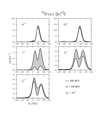
Figure 1: Cross sections for the ¹⁶O(e,e’2p)¹⁴C process. We indicated with $\epsilon$ the electron incoming energy, with $\omega$ the nuclear excitation energy, with $\gamma_{p_{2}}$ the emission angle of one proton and with $\gamma_{p_{1}}$ the emission angle of the second proton. The numbers in the panels indicate the quantum numbers of the ¹⁴C residual nucleus. We calculated only the final states that can be reached by emitting protons from the $p$ levels of the ¹⁶O nucleus. The gray bands are produced by the uncertainty on the theoretical inputs of the calculations, done with the same correlation function.

This final writing shows the fact that the transition matrix element can be written as a sum of power of $h$. The minimum power is zero, represented by the 1 in Eq. (4) and leading to the uncorrelated transition. The maximum power is $A$. In our approach we use the approximation of restricting the sum to the first power in $h$

$$\xi_{n}({\bf q})\longrightarrow\xi_{n}^{1}({\bf q}) = \langle\Phi_{n}|\,O({\bf q})\,(1+\sum_{i<j}\,h_{ij})\,|\Phi_{0}\rangle_{L}$$

$$= \langle\Phi_{n}(2p2h)|\,O({\bf q})\,\sum_{1<j}h(r_{1,j})\,|\Phi_{0}\rangle_{L}\,$$

$$+ \langle\Phi_{n}(2p2h)|\,O({\bf q})\,\sum_{1<i<j}\,h(r_{i,j})\,|\Phi_{0}\rangle_{L}\,\,.$$ (6)

In the last expression we show that, when the final state is composed by two particles in the continuum, the uncorrelated term does not act. For this reason there are only two types of terms. A first one where one of the coordinates of the function $h$ is also the coordinate where the external operator is acting on. This term leads to two-point diagrams. In the second type of terms, leading to three-point diagrams, the three coordinates are different. The presence of the two kinds of diagrams, necessary for the proper normalization of the final state of the nucleus, is a novelty of our calculations.

Figure 2: Correlation functions used in our calculations.

Figure 3: Cross sections for the ¹⁶O(e,e’2p)¹⁴C process. The various curves show the results obtained using the correlations of Fig. 2.

Figure 4: Cross sections for the ¹⁶O(e,e’2p)¹⁴C process calculated with the correlations shown in the lower right panel. In this calculations the two-body currents have not been considered.

Two nucleons can be emitted also by two-body electromagnetic currents. In our case two nucleons of the same type are emitted, therefore the meson exchange currents where a charged meson is exchanged do not contribute. There are also two-body currents where a chargeless meson is exchanged. These currents, implying the excitation of the $\Delta$, have been considered.

In Fig. 1 we show the ¹⁶O(e,e’2p)¹⁴C cross sections calculated for various final states. The shaded area is produced by the uncertainty on the input parameters. These uncertainties are related to the mean field describing the ground state, to the optical potential describing the wave functions of the emitted protons, to the energetics fixing the single particle energies, and, finally, to the $\gamma$-nucleon-$\Delta$ and the $\pi^{0}$-nucleon-$\Delta$ coupling constants. The uncertainty on the parameters describing the two-body currents produces the major effect. The 0⁺ states are rather insensitive to the two-body currents, while the 1⁺ state is dominated by the $\Delta$ excitation even at such relatively low excitation energy.

Our investigation on the sensitivity of the (e,e’2p) cross section to the details of the SRC, has been carried on by using the correlation functions shown in Fig. 2. The G (gaussian) and S3 correlations, have been taken from a Fermi Hypernetted Chain (FHNC) calculation done with semi-realistic interaction [5]. The V8 correlation is the scalar part of a state dependent correlation used in FHNC calculation done with a V8’ Argonne interaction plus three-body Urbana IX interaction [6].

The minimum of the G and S3 interaction is almost the same, while the V8 interaction has a deeper value. The V8 and S3 correlations overshoot the asymptotic value of 1 in the region between $r$=1 and 2 fm. The cross sections obtained with these correlations are shown in Fig. 3. Apart the result of the 1⁺ state dominated by the two-body currents, all the other results have common trends. First, one should notice that the use of different correlations does not change the shape of the angular distribution. Second, the cross sections obtained with the gaussian correlation, are larger than the other ones.

To understand this result, we have done a set of calculations with rather schematic correlations. These correlations are shown in the lower right panel of Fig. 4. The cross sections calculated with these correlations are shown in the other panels by lines of the same type. In these calculations the two-body $\Delta$ currents have not been included.

The box correlation indicated by the full line is our reference correlation. Lowering the minimum (dashed lines) does not produce a large effect. The insertion of a part which overshoots the asymptotic value reduces the cross section (dotted lines). An analogous effect is obtained by reducing the size of the box (dashed-dotted lines).

These results can be understood by remembering that the quantity entering in the cross section calculation is $h(r)=1-f^{2}(r)$ . The largest is the contribution of $h$ in Eq. (LABEL:eq:xi12), the largest is the cross section. The overshooting of the asymptotic value, generates a term in $h(r)$ of opposite sign with respect to the rest of the function, therefore the total contribution to the integral becomes smaller. The same effect can be obtained by reducing the size of the box as it is shown by the dashed dotted lines.

The information about the SRC can be obtained only by a quantitative comparison between theoretical predictions and experimental data. Qualitative features, such as the shape of the angular distributions, are not sensitive to the details of the SRC. Unfortunately a precise quantitative evaluation of the (e,e’2p) cross sections is linked to theoretical framework used to calculate it, and to the uncertainties in the required theoretical input. It appears clear that these kind of experiments cannot be considered as the ultimate tool able to pin down exactly the characteristics of the SRC correlations. They should instead be considered as another, useful and interesting, element of a puzzle, that together with elastic, inclusive and one-nucleon emission experiments we are trying to describe in a unique and coherent theoretical framework.

References

- [1] S.R. Mokhtar, G. Co’ and A.M. Lallena, Phys. Rev. C 62, 067304 (2000).
- [2] G. Co’ and A. M. Lallena, Ann. Phys. (N.Y.) 287, 101 (2001).
- [3] M. Anguiano, G. Co’, A. M. Lallena and S.R. Mokhtar, Ann. Phys. (N.Y.) 296, 235 (2002).
- [4] S. R. Mokhtar, M. Anguiano, G. Co’ and A. M. Lallena, Ann. Phys. (N.Y.) 292, 67 (2001).
- [5] F. Arias de Saavedra, G. Co’, A. Fabrocini and S. Fantoni, Nucl. Phys. A 605, 359 (1996).
- [6] A. Fabrocini, F. Arias de Saavedra and G. Co’, Phys. Rev. C 61, 044302 (2000).