Relativistic Mean Field Model with Generalized Derivative Nucleon-Meson Couplings

Abstract

The quantum hadrodynamics (QHD) model with minimal nucleon-meson couplings is generalized by introducing couplings of mesons to derivatives of the nucleon field in the Lagrangian density. This approach allows an effective description of a state-dependent in-medium interaction in the mean-field approximation. Various parametrizations for the generalized couplings are developed and applied to infinite nuclear matter. In this approach, scalar and vector nucleon self-energies depend on both density and momentum similarly as in the Dirac-Brueckner theory. The Schrödinger-equivalent optical potential is much less repulsive at high nucleon energies as compared to standard relativistic mean field models and thus agrees better with experimental findings. The derivative couplings in the extended model have significant effects on the properties of symmetric nuclear matter and neutron matter.

I Introduction

Properties of nuclear matter and finite nuclei have been described with great success by relativistic mean field (RMF) models in recent years Wal74 ; Rin96 ; Ser86 ; Ser92 ; Gam90 ; Ruf88 ; Rei86 ; Hor81 ; Chi77 . These models provide a novel saturation mechanism, an explanation of the strong spin-orbit interaction, and a natural energy dependence of the optical potential. They are often referred to as quantum hadrodynamics (QHD) since nuclear systems are described in these quantum field theories in terms of interacting hadrons, i.e. nucleon and meson fields. Lagrangians have been proposed in simple versions about 25 years ago Wal74 , and since then there have been many different treatments, extensions and applications.

There are basically two approaches of QHD, which one may call microscopic and phenomenological, respectively. The microscopic method is the Dirac-Brueckner (DB) approach deJ98 ; Seh97 ; Hub95 ; Boe94a ; Boe94b ; Fri94 ; Li92 ; deJ91 ; Bro90 ; Bot90 ; Mue88 ; Hor87 ; tHM87 ; Ana83 which tries to connect nucleon-nucleon scattering with finite nuclear systems via many-body theory. The effective Lagrangian has a simple form where nucleons and mesons couple in a minimal way. The coupling constants are fitted to NN scattering observables via the relativistic T-matrix approach. Then nuclear matter is treated in the Brueckner approximation and an effective in-medium interaction is extracted. The relativistic Brueckner approach successfully achieves saturation for nuclear matter which was not possible in non-relativistic methods with only two-body forces. Nucleon self energies $\Sigma_{i}$ ($i=$ scalar, vector, tensor, …) in the DB approach are both density and momentum dependent. Below the Fermi momentum $k_{F}$ the momentum dependence is found to be not very strong but above $k_{F}$ it corresponds to the momentum dependence in the empirical optical potential. While the DB method is very successful in describing infinite nuclear matter, it is very difficult to apply to finite nuclei without drastic approximations, e.g. the local density approximation (LDA). In order to describe detailed properties of finite nuclei some adjustements have to be introduced Boe94b ; Hof01 ; Had93 ; Bro92 .

In the phenomenological approach QHD is applied directly to nuclear systems without reference to NN scattering. Simple many-body approximations, usually the mean field approximation without exchange and correlation contributions, are employed. The coupling strengths of the mesons are directly adjusted to saturation properties of nuclear matter. In the original approach proposed by Walecka Wal74 the self energies are proportional to the corresponding densities. It was found that in this approach with linear meson-nucleon couplings properties of nuclear matter are not satisfactory away from saturation (too large incompressibility and too small effective mass) and finite nuclei are not described well. In order to improve the description the QHD Lagrangian has to be extended to include medium and state dependent effects in an effective way. This has been achieved by adding non-linear and higher order interaction terms to the Lagrangian or assuming density-dependent couplings of the nucleon and meson fields.

Non-linear models are the most prominent approach, in which cubic and quartic self-interactions of the $\sigma$-meson are introduced. This extension was proposed by Boguta and Bodmer Bog77 in order to lower the incompressibility of nuclear matter. Later the approach was extended to other meson fields Bod91 . Various parametrizations have been introduced which provide a good description of a whole range of nuclei Lal97 ; Sug94 ; Ruf88 ; Rei86 ; Sha00 . Replacing the minimal coupling of the $\sigma$-meson to the nucleon by a derivative coupling, Zimanyi and Moszkowski (ZM) obtained a particular non-linear $\sigma$-coupling after rescaling of the nucleon field Zim90 . Although this approach leads to a small incompressibility of nuclear matter, the effective nucleon mass turns out to be rather large, and, correspondingly, the spin-orbit interaction is too small. The ZM model with further extensions was studied in detail in Mit02 ; vCh00 ; Del94 . Recently, this class of approaches has been put on a more systematic basis in the effective field theories (EFT) where the possible terms and their importance are systematically categorized Fur00b ; Fur98 ; Fur97 ; Del01 ; Del99 .

An alternative approach assumes a density dependence of the coupling vertices Len95 ; Fuc95 ; Typ99 . This extension is suggested by DB theory. However, in a thermodynamically consistent and Lorentz covariant model, the couplings cannot depend parametrically on the density. They have to be lorentz-scalar functionals of the field operators. Then the Euler-Lagrange variational equations lead to so-called rearragement contributions in the self-energies. The first serious parametrization for finite nuclei was developed in Typ99 where a dependence of the couplings on the vector density (VDD) was found to work best. It was shown that good results can be obtained in the whole chart of nuclei, comparable to the best non-linear models. Recently, a new parametrization within the VDD approach has been developed Nik02 . These models can be considered in the general framework of density-functional theory which is given here in terms of the density dependent vertex functions. This connection is rather close, since the density dependence is motivated by DB theory which includes exchange and correlation terms.

Generally it seems desirable to describe the structure of nuclei and nuclear reactions in a common framework. This implies that one also needs the momentum dependence of the self energies at least for momenta above the Fermi surface. Empirically these are well studied in Dirac phenomenology by fitting scalar and vector potentials to elastic proton nucleus scattering data Ham90 ; Coo93 . It is found that the optical potential becomes repulsive with increasing energy but levels off at about 1 GeV. Optical potentials extracted from standard RMF models are much too large and increase linearly at high energies. Recently, a reasonable description of proton-nucleus scattering and an improved optical potential has been obtained by multiplying the self-energies from RMF calculations of finite nuclei with functions that depend explicitly on the proton energy Typ02 . However, the consistency of the theory is lost and the change of the energy dependence at different medium densities is not properly taken into account in this approach. The momentum dependence of the interaction also becomes important in the description of heavy-ion collisions. Several parametrizations for a parametric momentum dependence of the potentials have been developed in different approaches Dan00 ; Lee97 ; Li93 ; Mar94 ; Web93 ; Web92 .

So far, extensions of the RMF models concentrated on the effective density dependence of the in-medium interaction since they were mostly applied to the description of finite nuclei. If one goes beyond the mean field approximation momentum dependent self energies will emerge naturally. Recently, it was shown, that an energy-dependence of the self-energies can improve the level density close to the Fermi surface of finite nuclei Vre02 . In this RMF model, dynamical effects from the coupling of the single particle motion to collective surface vibrations are taken into account in a phenomenological approach. However, the energy-dependence was introduced only parametrically into the self-energies destroying the covariance of the theory. In order to retain the simple structure of the equations known from the RMF approximation one can imagine that it is desirable to modify the QHD Lagrangian in such a way that it leads to momentum dependent self energies already in the mean field approximation. In this work we propose such a class of Lagrangians with generalized derivative meson-nucleon couplings. The various types of possible couplings will have characteristic consequences in the field equations. Here we limit ourselves to the study of infinite nuclear matter within the derivative coupling (DC) model in order to demonstrate the main effects and the limitations of the approach. The results can serve as a foundation for a later application of the model to finite nuclei. Although derivative couplings have been investigated in simple approaches before, they were essentially cast into density-dependent forms, e.g. by rescaling the fields as in the ZM model. In EFT models contributions containing derivatives of the density are included, but generally they do not lead to a momentum dependence of the self energies and they do not affect properties of nuclear matter.

The paper is organized as follows. In Sec. II the the Lagrangian of the DC model is introduced and the field equation for mesons and nucleons are derived in the mean field approximation. In the following section the DC model is applied to infinite nuclear matter and expressions for basic quantities are derived. Three parametrizations are developed in Sec. IV and the resulting properties of symmetric and asymmetric nuclear matter are compared to standard RMF models. Finally, we summarize and give an outlook in Sec.V.

II Lagrangian density and field equations

The description of nuclear systems in QHD starts from a Lagrangian density $\mathcal{L}$ that contains nucleons and mesons as degrees of freedom. In case of symmetric nuclear matter it is sufficient to include isoscalar $\sigma$- and $\omega$-mesons. However, for asymmetric matter and finite nuclei, isovector mesons have to be added. It is customary to consider only the vector $\rho$-meson but for the sake of completeness we also take the scalar $\delta$-meson into account. The standard approach is to couple the nucleons minimally to the mesons. In case of the isoscalar mesons this leads to vertices of the form $\bar{\psi}\psi\sigma$ and $\bar{\psi}\gamma^{\mu}\psi\omega_{\mu}$ corresponding to the linear Walecka model.

The idea of the DC model is to introduce explicit couplings of the mesons to the first derivative of the nucleon field $\psi$, e.g. $\bar{\psi}i\partial_{\mu}\psi$ or $\bar{\psi}\gamma^{\mu}i\partial_{\mu}\psi$. The derivate $i\partial_{\mu}$ in the new coupling vertices is actually replaced by the covariant derivative $iD_{\mu}$ as it appears in the usual kinetic contribution to the Lagrangian. In the current model we consider couplings to the covariant derivative of the nucleon field which are linear or quadratic in the $\sigma$- and $\omega$-meson fields. For simplicity for the $\delta$- and $\rho$-mesons only linear couplings are taken into account. Of course, the standard minimal couplings are retained in the DC model.

On these conditions the Lagrangian density in the DC model assumes the form

$$\mathcal{L}=\frac{1}{2}\left[\bar{\psi}\Gamma_{\mu}iD^{\mu}\psi+\overline{(iD^{\mu}\psi)}\Gamma_{\mu}\psi\right]-\bar{\psi}\left(m-\Gamma_{\sigma}\sigma-\Gamma_{\delta}\vec{\tau}\cdot\vec{\delta}\right)\psi+{\cal L}_{m}$$ (1)

with the covariant derivative

$$iD_{\mu}=i\partial_{\mu}-\Gamma_{\omega}\omega_{\mu}-\Gamma_{\rho}\vec{\tau}\cdot\vec{\rho}_{\mu}\>.$$ (2)

The minimal coupling of the nucleons with mass $m$ to the mesons $i=\sigma$, $\omega$, $\delta$, $\rho$ of mass $m_{i}$ is specified by coupling strengths $\Gamma_{i}$. The contribution

$$\mathcal{L}_{m} = \frac{1}{2}\left[\partial^{\mu}\sigma\partial_{\mu}\sigma-m_{\sigma}^{2}\sigma^{2}+\partial^{\mu}\vec{\delta}\cdot\partial_{\mu}\vec{\delta}-m_{\delta}^{2}\vec{\delta}\cdot\vec{\delta}\right.$$

$$\left.-\frac{1}{2}G^{\mu\nu}G_{\mu\nu}+m_{\omega}^{2}\omega^{\mu}\omega_{\mu}-\frac{1}{2}\vec{H}^{\mu\nu}\cdot\vec{H}_{\mu\nu}+m_{\rho}^{2}\vec{\rho}^{\mu}\cdot\vec{\rho}_{\mu}\right]$$

to the total Lagrangian density $\mathcal{L}$ with field tensors

$$G_{\mu\nu}=\partial_{\mu}\omega_{\nu}-\partial_{\nu}\omega_{\mu}\qquad\vec{H}_{\mu\nu}=\partial_{\mu}\vec{\rho}_{\nu}-\partial_{\nu}\vec{\rho}_{\mu}$$ (4)

describes the free meson fields. The Lagrangian density (1) is symmetrized in the covariant derivative of the nucleon field to obtain field equations for $\psi$ and $\bar{\psi}$ that are related by a simple adjungation.

In constrast to the standard QHD Lagrangian density with Dirac $\gamma_{\mu}$ matrices in the kinetic term, the $4\times 4$ matrices

$$\Gamma_{\mu}=\gamma^{\nu}\left[\left(1+W\right)g_{\mu\nu}+X_{\mu\nu}\right]-T_{\mu}$$ (5)

are introduced in the DC model ($g_{\mu\nu}=\mbox{diag}(1,-1,-1,-1)$ is the metric tensor). They contain quantities

$$W=\mathcal{W}+\vec{\tau}\cdot\vec{\mathcal{W}}\qquad T_{\mu}=\mathcal{T}_{\mu}+\vec{\tau}\cdot\vec{\mathcal{T}}_{\mu}\qquad X_{\mu\nu}=\mathcal{X}_{\mu\nu}+\vec{\tau}\cdot\vec{\mathcal{X}}_{\mu\nu}$$ (6)

which are parametrized up to quadratic terms in the isoscalar meson fields

$$\mathcal{W}=\frac{\Gamma_{\sigma}^{(1)}}{m}\sigma-\frac{\Gamma^{(2)}_{\sigma}}{m^{4}}m_{\sigma}^{2}\sigma^{2}+\frac{\Gamma^{(2a)}_{\omega}}{m^{4}}m_{\omega}^{2}\omega^{\mu}\omega_{\mu}$$ (7)

$$\mathcal{T}_{\mu}=\frac{\Gamma_{\omega}^{(1)}}{m}\omega_{\mu}\qquad\mathcal{X}_{\mu\nu}=\frac{\Gamma^{(2b)}_{\omega}}{m^{4}}m_{\omega}^{2}\omega_{\mu}\omega_{\nu}$$ (8)

and linear terms in the isovector meson fields

$$\vec{\mathcal{W}}=\frac{\Gamma_{\delta}^{(1)}}{m}\vec{\delta}\qquad\vec{\mathcal{T}}_{\mu}=\frac{\Gamma_{\rho}^{(1)}}{m}\vec{\rho}_{\mu}\qquad\vec{\mathcal{X}}_{\mu\nu}=0\>.$$ (9)

The fields $W$, $T_{\mu}$, and $X_{\mu\nu}$ describe the coupling of the meson fields to the derivative of the nucleon field. The term $\mathcal{W}$ is similar to the extension of the ZM model and leads to a density dependence of the effective self energies. As will be seen later, the terms $\mathcal{T}_{\mu}$ and $\mathcal{X}_{\mu\nu}$ are the essential terms to give a momentum dependence to the scalar and vector self energies, respectively. Since the covariant derivative is used in (1), there appear also higher order nonlinear couplings to the nucleon field in the Lagrangian density.

In addition to the four coupling constants $\Gamma_{i}$ in $\mathcal{L}$ specifying the minimal nucleon-meson couplings, seven new couplings constants ($\Gamma_{\sigma}^{(1)}$, $\Gamma_{\sigma}^{(2)}$, $\Gamma_{\omega}^{(1)}$, $\Gamma_{\omega}^{(2a)}$, $\Gamma_{\omega}^{(2b)}$, $\Gamma_{\delta}^{(1)}$, $\Gamma_{\rho}^{(1)}$) appear. For the sake of convenience, mass factors are introduced to obtain pure numbers for the new coupling constants. The large number of new couplings makes the Lagrangian of the DC model very flexible. If the new coupling constants vanish the matrix $\Gamma_{\mu}$ (5) reduces to the usual $\gamma_{\mu}$ matrix and we recover the original QHD Lagrangian density with only mininal couplings. In comparison to the widely employed models with non-linear selfcouplings of the $\sigma$-meson ($\sigma$-meson and $\omega$-meson) there are five (four) additional free parameters in the DC model.

The non-linear or density-dependent RMF models discussed in the introduction are not a simple subcase of the present DC models. They could be included by making the couplings $\Gamma_{i}$ density-dependent or replacing them by polynomials in $\sigma$ and $\omega_{\mu}$. We do not want ot make this further extension. As will be seen later, the higher order terms in eqs. (7) and (8) produce similar effects as such additional terms.

The field equations of nucleons and mesons are derived from the corresponding Euler-Lagrange equations. In the mean field approximation the meson fields are treated as classical fields by replacing them with their expectation values. Only positive energy states of the nucleons are taken into account in the calculation of the densities (no-sea approximation). Symmetries of the nuclear system can lead to a considerable simplification the equations in the actual calculation, e.g. in infinite nuclear matter.

The field equation of the nucleons

$$\Gamma_{\mu}iD^{\mu}\psi-\left(m-\Gamma_{\sigma}\sigma-\Gamma_{\delta}\vec{\tau}\cdot\vec{\delta}\right)\psi+\frac{1}{2}\left(i\partial^{\mu}\Gamma_{\mu}\right)\psi=0$$ (10)

can be transformed to the usual Dirac form

$$\left[\gamma^{\mu}(i\partial_{\mu}-\Sigma_{\mu})-(m-\Sigma)\right]\psi=0$$ (11)

by introducing the scalar self energy

$$\Sigma=S-T_{\mu}i\partial^{\mu}$$ (12)

and the vector self energy

$$\Sigma_{\mu}=V_{\mu}-Wi\partial_{\mu}-X_{\mu\nu}i\partial^{\nu}$$ (13)

with

$$S=\Gamma_{\sigma}\sigma+\Gamma_{\delta}\vec{\tau}\cdot\vec{\delta}+T_{\mu}\left(\Gamma_{\omega}\omega^{\mu}+\Gamma_{\rho}\vec{\tau}\cdot\vec{\rho}^{\mu}\right)-\frac{1}{2}(i\partial^{\mu}T_{\mu})$$ (14)

and

$$V_{\mu}=[(1+W)g_{\mu\nu}+X_{\mu\nu}]\left(\Gamma_{\omega}\omega^{\nu}+\Gamma_{\rho}\vec{\tau}\cdot\vec{\rho}^{\nu}\right)-\frac{1}{2}(i\partial_{\mu}W)-\frac{1}{2}(i\partial^{\nu}X_{\mu\nu})\>.$$ (15)

The self energies (12) and (13) in the DC model are differential operators that act on the nucleon field. This fact is the essential extension in the new model with derivative couplings. Thus the self energies describe an interaction that contains a state dependence in addition to the medium dependence from the mesons fields. Additionally, both $S$ and $V_{\mu}$ depend on scalar and vector meson fields.

From the field equation (10) the continuity equation $\partial^{\mu}\hat{J}_{\mu}=0$ for the current density operator $\hat{J}_{\mu}=\bar{\psi}\Gamma_{\mu}\psi$ is immediately derived. Therefore, $\varrho=\langle\hat{J}_{0}\rangle$ has to be interpreted as the conserved baryon density in the DC model. The usual vector density $\varrho_{V}=\langle\bar{\psi}\gamma_{0}\psi\rangle$ is no longer a conserved quantity. Similar we find $\partial^{\mu}\hat{\vec{J}}_{\mu}=0$ for the isospin current density operator $\hat{\vec{J}}_{\mu}=\bar{\psi}\Gamma_{\mu}\vec{\tau}\psi$ .

The Lagrangian density $\mathcal{L}$ leads to the field equations for the isoscalar mesons

$$\partial^{\mu}\partial_{\mu}\sigma+m_{\sigma}^{2}\sigma\left(1+2\frac{\Gamma^{(2)}_{\sigma}}{m^{4}}\varrho_{s}^{D}\right) = \Gamma_{\sigma}\varrho_{s}+\frac{\Gamma_{\sigma}^{(1)}}{m}\varrho_{s}^{D}$$ (16)

$$\partial_{\mu}G^{\mu\nu}+m_{\omega}^{2}\omega_{\mu}\left[g^{\mu\nu}\left(1+2\frac{\Gamma^{(2a)}_{\omega}}{m^{4}}\varrho_{s}^{D}\right)+\frac{\Gamma^{(2b)}_{\omega}}{m^{4}}\left(t^{D\mu\nu}+t^{D\nu\mu}\right)\right] = \Gamma_{\omega}J^{\nu}+\frac{\Gamma_{\omega}^{(1)}}{m}j^{D\nu}$$ (17)

and for the isovector mesons

$$\partial^{\mu}\partial_{\mu}\vec{\delta}+m_{\delta}^{2}\vec{\delta} = \Gamma_{\delta}\vec{\varrho}_{s}+\frac{\Gamma_{\delta}^{(1)}}{m}\vec{\varrho}_{s}^{D}$$ (18)

$$\partial_{\mu}\vec{H}^{\mu\nu}+m_{\rho}^{2}\vec{\rho}^{\nu} = \Gamma_{\rho}\vec{J}^{\nu}+\frac{\Gamma_{\rho}^{(1)}}{m}\vec{\jmath}^{D\nu}\>.$$ (19)

They contain additional terms as compared to the linear QHD model. The masses of the isoscalar mesons are no longer constant but become effectively density dependent. The minimal coupling of nucleons and mesons leads to source terms with the usual scalar densities

$$\varrho_{s}=\langle\bar{\psi}\psi\rangle\qquad\vec{\varrho}_{s}=\langle\bar{\psi}\vec{\tau}\psi\rangle\>,$$ (20)

and the new current densities

$$J_{\mu}=\langle\bar{\psi}\Gamma_{\mu}\psi\rangle\qquad\vec{J}_{\mu}=\langle\bar{\psi}\Gamma_{\mu}\vec{\tau}\psi\rangle$$ (21)

which depend on the usual vector current densities

$$j_{\mu}=\langle\bar{\psi}\gamma_{\mu}\psi\rangle\qquad\vec{\jmath}_{\mu}=\langle\bar{\psi}\gamma_{\mu}\vec{\tau}\psi\rangle$$ (22)

and the scalar densities (see appendix A).

Additional source terms proportional to $\Gamma_{\sigma}^{(1)}$, $\Gamma_{\omega}^{(1)}$, $\Gamma_{\delta}^{(1)}$, and $\Gamma_{\rho}^{(1)}$ appear in the field equations with the derivative scalar densities

$$\varrho_{s}^{D} = \frac{1}{2}\langle\left[\bar{\psi}\gamma^{\mu}iD_{\mu}\psi+\overline{(iD_{\mu}\psi)}\gamma^{\mu}\psi\right]\rangle=g^{\mu\nu}t_{\mu\nu}^{D}$$ (23)

$$\vec{\varrho}_{s}^{D} = \frac{1}{2}\langle\left[\bar{\psi}\gamma^{\mu}iD_{\mu}\vec{\tau}\psi+\overline{(iD_{\mu}\psi)}\gamma^{\mu}\vec{\tau}\psi\right]\rangle=g^{\mu\nu}\vec{t}_{\mu\nu}^{D}$$ (24)

and the derivative current densities

$$j^{D}_{\mu} = \frac{1}{2}\langle\left[\bar{\psi}iD_{\mu}\psi+\overline{(iD_{\mu}\psi)}\psi\right]\rangle$$ (25)

$$\vec{\jmath}^{D}_{\mu} = \frac{1}{2}\langle\left[\bar{\psi}iD_{\mu}\vec{\tau}\psi+\overline{(iD_{\mu}\psi)}\vec{\tau}\psi\right]\rangle\>.$$ (26)

As shown, the scalar densities (23) and (24) can also be expressed in terms of the derivative tensor densities

$$t^{D}_{\mu\nu} = \frac{1}{2}\langle\left[\bar{\psi}\gamma_{\mu}iD_{\nu}\psi+\overline{(iD_{\nu}\psi)}\gamma_{\mu}\psi\right]\rangle$$ (27)

$$\vec{t}^{D}_{\mu\nu} = \frac{1}{2}\langle\left[\bar{\psi}\gamma_{\mu}iD_{\nu}\vec{\tau}\psi+\overline{(iD_{\nu}\psi)}\gamma_{\mu}\vec{\tau}\psi\right]\rangle$$ (28)

which are not symmetric in the Lorentz indices. More explicit expressions for the densities can be found in appendix A.

III Application to infinite nuclear matter

Infinite nuclear matter in its ground state is a homogeneous, isotropic and stationary system. Because of these symmetries, the set of field equations simplifies considerably. Densities do not depend on space-time coordinates and only the time-like component of the currents remains. Correspondingly, the meson fields are constant and the spatial components of the vector meson field vanish. Additionally, only the third component in isospin of the isovector densities and isovector meson fields remains. The matrix $\Gamma_{\mu}$ is diagonal in isospin space and it is useful to introduce the abbreviations

$$\Gamma_{0\pm}=\gamma_{0}\left(1+W_{\pm}+X_{00\pm}\right)-T_{0\pm}\qquad\Gamma_{i\pm}=\gamma_{i}\left(1+W_{\pm}\right)\quad i=1,2,3$$ (29)

for the time-like and space-like components of $\Gamma_{\mu}$ with the quantities

$$W_{\pm}=\mathcal{W}\pm\left(\vec{\mathcal{W}}\right)_{3}\qquad T_{0\pm}=\mathcal{T}_{0}\pm\left(\vec{\mathcal{T}}_{0}\right)_{3}\qquad X_{00\pm}=\mathcal{X}_{00}\pm\left(\vec{\mathcal{X}}_{00}\right)_{3}$$ (30)

where the case of protons is denoted by $+$ and neutrons by $-$, respectively. The momentum independent contributions to the self energies (12) and (13) are given by

$$S_{\pm}=\Gamma_{\sigma}\sigma\pm\Gamma_{\delta}(\vec{\delta})_{3}+T_{0\pm}\left[\Gamma_{\omega}\omega_{0}\pm\Gamma_{\rho}(\vec{\rho}_{0})_{3}\right]$$ (31)

and

$$V_{0\pm}=(1+W_{\pm}+X_{00\pm})\left[\Gamma_{\omega}\omega_{0}\pm\Gamma_{\rho}\left(\vec{\rho}_{0}\right)_{3}\right]\>.$$ (32)

The meson fields are directly obtained from the field equations (16) - (19) for given densities.

III.1 Solutions of the generalized Dirac equation

In order to calculate the various densities appearing in the field equations we first have to find the nucleon field from the the generalized Dirac equation with self-energies that are differential operators in the DC model. Solutions of the nucleon field equation are found with the plane wave ansatz

$$\psi(\vec{p},\sigma,\tau)=u(\vec{p},\sigma,\tau)\exp\left(-ip_{\mu}x^{\mu}\right)$$ (33)

for a nucleon with four momentum $p_{\mu}=(E,\vec{p})$ and positive energy $E$. Spin and isospin quantum numbers are specified by $\sigma$ and $\tau$. The scalar self energy

$$\Sigma_{\pm}=S_{\pm}-T_{0\pm}E$$ (34)

and the vector self energy

$$\Sigma_{0\pm}=V_{0\pm}-(W_{\pm}+X_{00\pm})E$$ (35)

for nucleons in nuclear matter are explicitly energy dependent in the DC model. They decrease with energy for positive $T_{0\pm}$ and $(W_{\pm}+X_{00\pm})$. Of course, this linear dependence will give a reasonable description of realistic self energies only for not too high energies. The quantities $T_{0\pm}$, $W_{\pm}$, and $X_{00\pm}$ increase with increasing density and the energy dependence of the self energies becomes stronger. This behaviour also leads to a limitation in the density range where the DC model can be applied because of the increase of the Fermi momentum. Since the energy $E$ already contains the rest mass $m$ of the nucleon the self energies are rather insensitive to the nucleon energy if $E<m$. The energy dependence itself is density dependent and it is different for protons and neutrons if $\Gamma_{\delta}^{(1)}\neq 0$ or $\Gamma_{\rho}^{(1)}\neq 0$. The ansatz (33) in the Dirac equation (11) leads to the condition

$$\left(\begin{array}[]{cc}\tilde{M}_{\tau}-\tilde{E}_{\tau}&\vec{\sigma}\cdot\vec{\tilde{p}}_{\tau}\\ \vec{\sigma}\cdot\vec{\tilde{p}}_{\tau}&-\tilde{M}_{\tau}-\tilde{E}_{\tau}\end{array}\right)u(\vec{p},\sigma,\tau)=0$$ (36)

for the spinor $u(\vec{p},\sigma,\tau)$ if the abbreviations

$$\tilde{M}_{\tau} = m-S_{\tau}+T_{0\tau}E$$ (37)

$$\tilde{E}_{\tau} = (1+W_{\tau}+X_{00\tau})E-V_{0\tau}$$ (38)

$$\vec{\tilde{p}}_{\tau} = (1+W_{\tau})\vec{p}$$ (39)

are introduced. These quantities carry the index $\tau=\pm$ because the fields are not necessarily equal for protons and neutrons in asymmetric nuclear matter. The dispersion relation

$$\tilde{M}_{\tau}^{2}=\tilde{E}_{\tau}^{2}-\tilde{p}_{\tau}^{2}$$ (40)

connects the energy

$$\tilde{E}_{\tau}=\frac{1}{\sqrt{1-B^{2}}}\left(A_{\tau}B_{\tau}+\sqrt{A_{\tau}^{2}+\tilde{p}_{\tau}^{2}}\right)$$ (41)

and mass

$$\tilde{M}_{\tau}=\frac{1}{\sqrt{1-B_{\tau}^{2}}}\left(A_{\tau}+B_{\tau}\sqrt{A_{\tau}^{2}+\tilde{p}_{\tau}^{2}}\right)\>.$$ (42)

where the constants

$$A_{\tau}=\frac{m-S_{\tau}+B_{\tau}V_{0\tau}}{\sqrt{1-B_{\tau}^{2}}}\qquad B_{\tau}=\frac{T_{0\tau}}{1+W_{\tau}+X_{00\tau}}$$ (43)

have been introduced. Not only the energy $\tilde{E}_{\tau}$, but also the mass $\tilde{M}_{\tau}$, depends on the momentum, the density and isospin. Obviously, reasonable solutions of the Dirac equation exist only for $-1<B_{\tau}<1$ and $1+W_{\tau}+X_{00\tau}\neq 0$. The energy in the four-momentum of the nucleon in (33) is given by

$$E_{\tau}=(1+W_{\tau}+X_{00\tau})^{-1}\left[V_{0\tau}+\frac{1}{\sqrt{1-B_{\tau}^{2}}}\left(A_{\tau}B_{\tau}+\sqrt{A_{\tau}^{2}+\tilde{p}_{\tau}^{2}}\right)\right]\>.$$ (44)

Solutions of equation (36) are found to be

$$u(\vec{p},\sigma,\tau)=\sqrt{\frac{\tilde{M}_{\tau}+\tilde{E}_{\tau}}{2[(1+W_{\tau}+X_{00\tau})\tilde{E}_{\tau}-T_{0\tau}\tilde{M}_{\tau}]}}\left(\begin{array}[]{c}\chi_{\sigma}\\ \frac{\vec{\sigma}\cdot\vec{\tilde{p}}_{\tau}}{\tilde{M}_{\tau}+\tilde{E}_{\tau}}\chi_{\sigma}\end{array}\right)\xi_{\tau}$$ (45)

with spin and isospin eigenfunctions $\chi_{\sigma}$ and $\xi_{\tau}$. The normalization of these spinors is discussed in appendix B.

Negative energy solutions are obtained by a similar procedure.. Then the theory can be quantized in the usual way by expanding the nucleon field operator in terms of the complete set of solutions and imposing anticommutation relations for the creation and annihilation operators. However, in the mean field solution we do not need to carry out this standard procedure in detail here.

III.2 Densities

The densities that appear in the field equations are obtained by a summation over all occupied states in nuclear matter up to the Fermi momentum $p^{F}_{\tau}$ for protons and neutrons, respectively. In the no-sea approximation only states of positive energy are considered. Proton and neutron constribution to the various densities can be obtained with the help of the projection operator $P_{\tau}=(1+\tau(\vec{\tau})_{3})/2$, e.g., the total baryon density

$$\varrho=J_{0}=\varrho_{+}+\varrho_{-}$$ (46)

and the third component of the isospin density

$$\left(\vec{J}_{0}\right)_{3}=\varrho_{+}-\varrho_{-}$$ (47)

are the sum and the difference of the proton and neutron densities

$$\varrho_{\tau}=\langle\bar{\psi}\Gamma_{0}P_{\tau}\psi\rangle\>,$$ (48)

respectively. The other isoscalar and isovector densities are related to the corresponding proton and neutron densities in a similar manner. Considering the normalization of the solutions of the Dirac equation all densities can be expressed in terms of the three fundamental integrals

$$I^{\tau}_{1} = \int_{0}^{\tilde{p}^{F}_{\tau}}d\tilde{p}_{\tau}\>\tilde{p}_{\tau}^{2}=\frac{1}{3}(\tilde{p}^{F}_{\tau})^{3}$$ (49)

$$I^{\tau}_{2} = \int_{0}^{\tilde{p}^{F}_{\tau}}d\tilde{p}_{\tau}\>\frac{\tilde{p}_{\tau}^{2}}{\sqrt{A_{\tau}^{2}+\tilde{p}_{\tau}^{2}}}=\frac{1}{2}\left[\tilde{p}^{F}_{\tau}E^{F}_{\tau}-A_{\tau}^{2}\ln\frac{\tilde{p}^{F}_{\tau}+E^{F}_{\tau}}{A_{\tau}}\right]$$ (50)

$$I^{\tau}_{3} = \int_{0}^{\tilde{p}^{F}_{\tau}}d\tilde{p}_{\tau}\>\tilde{p}_{\tau}^{2}\sqrt{A_{\tau}^{2}+\tilde{p}_{\tau}^{2}}=\frac{3E^{F}_{\tau}}{4}I^{\tau}_{1}+\frac{A_{\tau}^{2}}{4}I^{\tau}_{2}$$ (51)

with $\tilde{p}^{F}_{\tau}=(1+W)p^{F}_{\tau}$ and $E^{F}_{\tau}=\sqrt{A_{\tau}^{2}+(\tilde{p}^{F}_{\tau})^{2}}$. The proton and neutron densities are then given by

$$\varrho_{\tau}=\langle\bar{\psi}\Gamma_{0}P_{\tau}\psi\rangle=\frac{\kappa}{2\pi^{2}}(1+W)^{-3}I^{\tau}_{1}=\frac{1}{3\pi^{2}}\left(p^{F}_{\tau}\right)^{3}$$ (52)

with the spin degeneracy factor $\kappa=2$. This relation defines the corresponding Fermi momentum $p^{F}_{\tau}$ for a given nucleon density. Immediately, we obtain the scalar density

$$\varrho_{s\tau}=\langle\bar{\psi}P_{\tau}\psi\rangle=C_{\tau}^{-1}\left[B_{\tau}I^{\tau}_{1}+A_{\tau}I^{\tau}_{2}\right]$$ (53)

and the current density

$$j_{0\tau}=\langle\bar{\psi}\gamma_{0}P_{\tau}\psi\rangle=C_{\tau}^{-1}\left[I^{\tau}_{1}+A_{\tau}B_{\tau}I^{\tau}_{2}\right]$$ (54)

with

$$C_{\tau}=\pi^{2}(1+W_{\tau}+X_{00\tau})(1+W_{\tau})^{3}(1-B_{\tau}^{2})\>.$$ (55)

With these results the relation

$$\varrho_{\tau}=(1+W_{\tau}+X_{00\tau})j_{0\tau}-T_{0\tau}\varrho_{s\tau}$$ (56)

is easily confirmed. Considering the relation (38) the derivative densities are most easily calculated from

$$j^{d}_{0\tau}=\langle\bar{\psi}E_{\tau}P_{\tau}\psi\rangle=(1+W_{\tau}+X_{00\tau})^{-1}\left(\varrho^{E}_{s\tau}+V_{0\tau}\varrho_{s\tau}\right)$$ (57)

and

$$t^{d}_{00\tau}=\langle\bar{\psi}\gamma_{0}E_{\tau}P_{\tau}\psi\rangle=(1+W_{\tau}+X_{00\tau})^{-1}\left(\varrho^{E}_{\tau}+V_{0\tau}j_{0\tau}\right)$$ (58)

where

$$\varrho^{E}_{s\tau}=\langle\bar{\psi}\tilde{E}_{\tau}P_{\tau}\psi\rangle=C_{\tau}^{-1}(1-B_{\tau}^{2})^{-\frac{1}{2}}\left[A_{\tau}(1+B_{\tau}^{2})I^{\tau}_{1}+A_{\tau}^{2}B_{\tau}I^{\tau}_{2}+B_{\tau}I^{\tau}_{3}\right]$$ (59)

and

$$\varrho^{E}_{\tau}=\langle\bar{\psi}\gamma_{0}\tilde{E}^{+}_{\tau}P_{\tau}\psi\rangle=C_{\tau}^{-1}(1-B_{\tau}^{2})^{-\frac{1}{2}}\left[2A_{\tau}B_{\tau}I^{\tau}_{1}+A_{\tau}^{2}B_{\tau}^{2}I^{\tau}_{2}+I^{\tau}_{3}\right]\>.$$ (60)

The scalar derivative density is deduced from

$$\varrho_{s\tau}^{d} = t_{\lambda\mu_{\tau}}^{d}g^{\lambda\mu}=\langle\bar{\psi}\gamma_{0}E_{\tau}P_{\tau}\psi\rangle-\langle\bar{\psi}\vec{\gamma}\cdot\vec{p}P_{\tau}\psi\rangle$$

$$= t_{00\tau}^{d}-(1+W_{\tau})^{-1}\left(\varrho^{E}_{\tau}-\varrho^{M}_{s\tau}\right)$$

with (92), the dispersion relation (40), and

$$\varrho^{M}_{s\tau}=\langle\bar{\psi}\tilde{M}_{\tau}P_{\tau}\psi\rangle=C_{\tau}^{-1}(1-B_{\tau}^{2})^{-\frac{1}{2}}\left[2A_{\tau}B_{\tau}I^{\tau}_{1}+A_{\tau}^{2}I^{\tau}_{2}+B_{\tau}^{2}I^{\tau}_{3}\right]\>.$$ (62)

Nuclear matter is characterized by its equation of state, i.e. the energy per nucleon or pressure as a function of the nucleon density. The energy density is calculated from the energy-momentum tensor

$$T^{\lambda\mu} = \sum_{\varphi}\frac{\partial\mathcal{L}}{\partial(\partial_{\lambda}\varphi)}\partial^{\mu}\varphi-g^{\lambda\mu}\mathcal{L}$$ (63)

where the sum runs over all fields ($\varphi=\psi,\bar{\psi},\sigma,\vec{\delta},\omega_{\nu},\vec{\rho}_{\nu}$). Since there are no contributions from the derivatives of the meson fields in nuclear matter the expectation value of the energy-momentum tensor reduces to

$$\langle T^{\lambda\mu}\rangle=\langle\bar{\psi}\Gamma^{\lambda}p^{\mu}\psi\rangle-g^{\lambda\mu}\langle\mathcal{L}\rangle$$ (64)

with

$$\langle\mathcal{L}\rangle=\frac{1}{2}\left[m_{\omega}^{2}\omega^{\mu}\omega_{\mu}+m_{\rho}^{2}\vec{\rho}^{\mu}\cdot\vec{\rho}_{\mu}-m_{\sigma}^{2}\sigma^{2}-m_{\delta}^{2}\vec{\delta}\cdot\vec{\delta}\right]\>.$$ (65)

Only the meson fields contribute to $\langle\mathcal{L}\rangle$ because the nucleon fields are solutions of the Dirac equation (10). With the help of equations (37), (38), and (92) the energy density

$$\varepsilon = \langle T_{00}\rangle=\langle\bar{\psi}\Gamma_{0}E_{0}\psi\rangle-\langle\mathcal{L}\rangle$$

$$= \sum_{\tau}\langle\bar{\psi}\left[\gamma_{0}(\tilde{E}_{\tau}+V_{0\tau})-(\tilde{M}_{\tau}-m+S_{\tau})\right]P_{\tau}\psi\rangle-\langle\mathcal{L}\rangle$$

$$= \sum_{\tau}\left[\varrho^{E}_{\tau}-\varrho^{M}_{s\tau}+(m-S_{\tau})\varrho_{s\tau}+V_{0\tau}j_{0\tau}\right]$$

$$-\frac{1}{2}\left[m_{\omega}^{2}\omega_{0}^{2}+m_{\rho}^{2}\vec{\rho}_{0}^{2}-m_{\sigma}^{2}\sigma^{2}-m_{\delta}^{2}\vec{\delta}^{2}\right]$$

and the pressure

$$p = \frac{1}{3}\sum_{i=1}^{3}\langle T_{ii}\rangle=\frac{1}{3}\langle\bar{\psi}\vec{\gamma}\cdot\vec{\tilde{p}}\psi\rangle+\langle\mathcal{L}\rangle$$

$$= \frac{1}{3}\sum_{\tau}\left(\varrho^{E}_{\tau}-\varrho^{M}_{s\tau}\right)+\frac{1}{2}\left[m_{\omega}^{2}\omega_{0}^{2}+m_{\rho}^{2}\vec{\rho}_{0}^{2}-m_{\sigma}^{2}\sigma^{2}-m_{\delta}^{2}\vec{\delta}^{2}\right]$$

are found. The DC model in the mean field approximation is thermodynamically consistent because the pressure (III.2) calculated from the energy-momentum tensor agrees with the thermodynamical pressure $p_{th}=\varrho^{2}\frac{d}{d\varrho}\left(\frac{\varepsilon}{\varrho}\right)$. Furthermore the relation

$$\varepsilon+p=\mu_{+}\varrho_{+}+\mu_{-}\varrho_{-}$$ (68)

is obtained with the chemical potentials

$$\mu_{\tau}=(1+W_{\tau}+X_{00\tau})^{-1}\left[V_{0\tau}+\frac{1}{\sqrt{1-B_{\tau}^{2}}}\left(A_{\tau}B_{\tau}+\sqrt{A_{\tau}^{2}+(\tilde{p}_{\tau}^{F})^{2}}\right)\right]$$ (69)

which are the energies (44) of the nucleons at the Fermi surface and the Hugenholtz-van Hove theorem Hug58 holds.

Determing the properties of nuclear matter in the DC model for a given density $\varrho$ and neutron-proton asymmetry $\alpha=\frac{\varrho_{n}-\varrho_{p}}{\varrho_{n}+\varrho_{p}}$ is more involved than in standard RMF models. The meson fields have to be determined from the densities which themselves depend on the meson fields. A self-consistent solution is achieved by iteratively solving the set of equations until convergence is reached.

III.3 Optical potential

The Schrödinger equivalent optical potential $V_{\rm opt}$ serves as a convenient means to characterize the in-medium interaction of a nucleon. It is obtained by recasting the Dirac equation (11) into a Schrödinger-like equation for the large (upper) component of the nucleon spinor. In the DC model the momentum $\vec{p}$ in the generalized Dirac equation is multiplied by a factor $(1+W_{\tau})$ in eq. (39). In order to start for the non-relativistic reduction from the usual form of the time-independent Dirac equation

$$\left[\vec{\alpha}\cdot\vec{p}+\beta\left(m-\Sigma^{\rm eff}_{\tau}\right)\right]\psi_{\tau}=\left(E-\Sigma_{0\tau}^{\rm eff}\right)\psi_{\tau}$$ (70)

the effective self energies

$$\Sigma^{\rm eff}_{\tau}=\frac{\Sigma_{\tau}+W_{\tau}m}{1+W_{\tau}}=\frac{S_{\tau}-T_{0\tau}E+W_{\tau}m}{1+W_{\tau}}$$ (71)

and

$$\Sigma_{0\tau}^{\rm eff}=\frac{\Sigma_{0\tau}+W_{\tau}E}{1+W_{\tau}}=\frac{V_{0\tau}-X_{00\tau}E}{1+W_{\tau}}$$ (72)

are introduced. They depend linearly on the nucleon energy $E$ if $T_{0\tau}\neq 0$ and $X_{00\tau}\neq 0$. Since $E$ contains the rest mass of the nucleon, there is only a small variation of the self-energies at small momenta of the nucleon. It is seen that the coupling vertices in the DC model with $\Gamma_{\omega}^{(1)}$, $\Gamma_{\rho}^{(1)}$, and $\Gamma_{\omega}^{(2b)}$ lead to the energy-dependent scalar and vector self-energies, respectively. In the DC model the energy dependence results from the coupling of the Lorentz-vector meson fields to the derivative of the nucleon field. The Lorentz-scalar meson fields do not lead to an energy dependence of the effective self energies. The modification of the initial Lagrangian (1) by the term $W$ alone does not introduce an energy dependence of the effective self energies. This resembles the ZM model in which the derivative coupling is a special case of the $W$ contribution in the DC model. By a rescaling of the nucleon wave function in the ZM model, the derivative coupling was essentially removed, leading to a nonlinear coupling of the nucleon field to the $\sigma$-meson without an energy dependence of the self energies.

The quantities $T_{0\tau}$ and $X_{00\tau}$ have different density dependencies. At low densities they are approximately proportional to the baryon density and the square of the baryon density, respectively. But with increasing density this proportionality is lost because of the nonlinearity of the meson field equations. Even without an energy dependence the effective self energies (71) and (72) in the DC model show a nontrivial density dependence.

There are various methods to derive the optical potential from the Dirac equation (70). Here, the definition

$$V_{\rm opt\tau}=\frac{E}{m}\Sigma_{0\tau}^{\rm eff}-\Sigma^{\rm eff}_{\tau}+\frac{1}{2m}\left[\left(\Sigma^{\rm eff}_{\tau}\right)^{2}-\left(\Sigma_{0\tau}^{\rm eff}\right)^{2}\right]$$ (73)

for the Schrödinger equivalent optical potential is used as in Refs. Lee97 . It has the property that $V_{\rm opt\tau}$ rises linearly with the energy $E$ of the nucleon if the self energies are energy independent. An alternative choice is the definition as used in Ref. Ham90 which corresponds to multiplying (73) by $m/E$. In Ref. Fel91 ; Li93 the optical potential is calculated from the difference of the energy $E$ of the nucleon in the medium and the kinetic energy of a free nucleon without interaction at the same momentum $\vec{p}$. This definition is more appropriate for a general relativistic definition of an optical potential but it is no longer a Schrödinger equivalent potential. It always leads to a constant optical potential for large nucleon momenta for energy independent self energies. For a meaningful comparison of optical potentials it is, of course, necessary to chose the same definition.

The optical potential (73) in the DC model is a quadratic function of the nucleon energy because the effective self energies (71) and (72) are linear functions of the energy. This behaviour is reasonable only in a limited range of energies and the model cannot be applied at arbitrarily high energies. But for nucleon energies up to about 1 GeV the linear dependence is a sufficient approximation. Indeed, self energies from Dirac phenomenology of proton scattering show an approximately linear decrease for small energies Ham90 ; Coo93 .

IV Parametrizations and properties of nuclear matter

The DC model introduces a large number of additional couplings as compared to the original RMF model with minimal meson-nucleon couplings and even with respect to usual non-linear models. The corresponding coupling constants have to be fixed by the limited number of nuclear matter properties. Here, we develop parametrizations within restricted versions of the DC model in order to investigate whether the model gives reasonable results.

Symmetric nuclear matter is essentially characterized by the binding energy per nucleon $E/A$ and the incompressibility $K$ at saturation density $\varrho_{\rm sat}$ where the pressure $p$ is zero. This leads to three conditions for the seven isoscalar coupling constants $\Gamma_{\sigma}$, $\Gamma_{\sigma}^{(1)}$, $\Gamma_{\sigma}^{(2)}$, $\Gamma_{\omega}$ $\Gamma_{\omega}^{(1)}$, $\Gamma_{\omega}^{(2a)}$, and $\Gamma_{\omega}^{(2b)}$. Furthermore, an adjustment of the relativistic effective mass $M^{\rm eff}=m-\Sigma^{\rm eff}$ at saturation density can be used to achieve a reasonable spin-orbit splitting in finite nuclei. A reduction of $M^{\rm eff}$ increases the spin-orbit splitting. The four isovector coupling constants $\Gamma_{\delta}$, $\Gamma_{\delta}^{(1)}$, $\Gamma_{\rho}$, and $\Gamma_{\rho}^{(1)}$ in the DC model determine the symmetry energy $J$ and its derivative with respect to the density which can be parametrized by $L=3\varrho\frac{dJ}{d\varrho}$. In all our parametrizations, the $\delta$-meson is not considered, which is common practice in most RMF parametrizations, because its contribution seems not to be well determined in parameter fits to properties of finite nuclei.

All our parametrizations of the DC models are fitted to give $E/A=-16.0$ MeV for the binding energy per nucleon at a saturation density of $\varrho_{\rm sat}=0.150$ fm^-3 with an incompressibility of $K=240$ MeV. These are reasonable values as compared to the properties of symmetric nuclear matter in other models. The parameters are adjusted to an effective nucleon mass at $\varrho_{\rm sat}$ of $M^{\rm eff}=0.6m$ close to the value of several relativistic mean field parametrizations with spin-orbit splittings of single-particle levels close to the experimental values. These four conditions require at least four isoscalar coupling constants in the model. The assumemd symmetry energy of $J=32$ MeV fixes one isovector coupling constant.

In the first parametrization (DC1) only the usual minimal meson-nucleon couplings with $\Gamma_{\sigma}$, $\Gamma_{\omega}$, and $\Gamma_{\rho}$ and the new couplings $\Gamma_{\sigma}^{(2)}$ and $\Gamma_{\omega}^{(2a)}$ are assumed to be non-zero. This leads to a model without energy-dependent effective self-energies because $T_{\mu}=0$ and $X_{\mu\nu}=0$. The non-zero quantity $W$ contains only contributions quadratic in the $\sigma$-meson and $\omega$-meson fields and correspondingly, these mesons acquire a density-dependent effective mass. The DC1 parametrization has the same number of parameters as the standard non-linear models with self-interactions of the $\sigma$-meson.

The second and third parameter set (DC2/DC3) are chosen to give a reasonable description of the Schrödinger equivalent optical potential of the nucleon in symmetric nuclear matter at saturation density $\varrho_{\rm sat}$. Since the optical potential extracted in Dirac phenomenology from proton-nucleus scattering becomes almost constant around the kinetic energy $E-m=1$ GeV of the nucleon, we adjust the coupling constants to exhibit a maximum of the potential at this energy. The DC model is not really applicable to higher energies because the empirical self-energies show a deviation from the linear energy-dependence and in our approach the optical potential is a quadratic function of the nucleon energy. The coupling constants $\Gamma_{\omega}^{(1)}$ and $\Gamma_{\omega}^{(2b)}$ have to be positive to generate a reduction of the self-energies with increasing nucleon energy. In order to keep the number of parameters small we require in this model the additional constraints $\Gamma_{\omega}^{(2a)}+\Gamma_{\omega}^{(2b)}=0$ and $\Gamma_{\sigma}^{(1)}=\Gamma_{\omega}^{(1)}$. For small densities this condition cancels the density dependence of the $\omega$-meson mass in eq. (17) and makes the coupling coefficients to the derivative densities equal in eqs. (16,17). Now the five independent isoscalar parameters are uniquely determined by five conditions.

In the parametrizations DC1 and DC2 the constant $\Gamma_{\rho}$ is fitted to give a symmetry energy of $J=32$ MeV wheras $\Gamma_{\rho}^{(1)}$ is assumed to be zero. The sets DC2 and DC3 share the same isoscalar coupling constants but in model DC3 the two coupling constants of the $\rho$-meson are adjusted to give both a symmetry energy of $J=32$ MeV and a derivative $L=40$ MeV of the symmetry energy at saturation density in symmetric nuclear matter. This value of $L$ is typical for non-relativistic Skyrme Hartree-Fock models. An increase of $\Gamma_{\rho}^{(1)}$ leads to a decrease of $\Gamma_{\rho}$ in order to give the same symmetry energy. Precise values for the coupling constants in all DC models are presented in Table 1.

Table 1: Coupling constants in the DC models. The nucleon mass is $m=939$ MeV and the meson masses are $m_{\sigma}=550$ MeV, $m_{\omega}=783$ MeV, and $m_{\rho}=763$ MeV.

model	$\Gamma_{\sigma}$	$\Gamma_{\omega}$	$\Gamma_{\rho}$	$\Gamma_{\sigma}^{(1)}$	$\Gamma_{\omega}^{(1)}$	$\Gamma_{\rho}^{(1)}$	$\Gamma_{\sigma}^{(2)}$	$\Gamma_{\omega}^{(2a)}$	$\Gamma_{\omega}^{(2b)}$
DC1	10.996338	12.831929	3.783530	0.000	0.000	0.000	84.77	12.30	0.00
DC2	10.536751	13.754212	3.917768	2.392	2.392	0.000	8.735	-211.54	211.54
DC3	10.536751	13.754212	0.943337	2.392	2.392	5.525	8.735	-211.54	211.54

Figure 1: Binding energy per nucleon for symmetric nuclear matter as a function of the nucleon density in various relativistic mean field parametrizations.

It is instructive to compare various properties of symmetric nuclear matter and neutron matter in the DC models with other typical relativistic mean field models, in particular with standard non-linear parametrizations and models with density-dependent couplings. Here we chose the parametrization NL3 Lal97 which contains tertic and quartic self-interactions of the $\sigma$-meson field and the set TM1 Sug94 which takes also self-interactions of the $\omega$-meson into account. The VDD model Typ99 assumes a dependence of meson-nucleon couplings on the vector density that generates so-called “rearrangement” contributions in the self-energies leading to a non-trivial density dependence. These parametrizations were obtained by fits to properties of finite nuclei and nuclear matter.

In Figure 1 the binding energy of symmetric nuclear matter is shown for different models as a function of the density. Below saturation density all parametrizations lead to almost identical results, but at higher densities there are characteristic differences. The DC1 model without energy dependent effective self energies is very similar to the NL3 parametrization with the non-linear self-interaction of the $\sigma$ meson. The effective density-dependence of the meson masses in the DC1 model with $\Gamma_{\sigma}^{(2)}\gg\Gamma_{\omega}^{(2a)}$ apparently leads to an effective density dependence of the scalar and vector self-energies that is comparable to the standard non-linear model. This is easily observed by comparing the effective coupling constants in symmetric nuclear matter. They are extracted from the self-energies according to

$$\Gamma_{\sigma}^{\rm eff}=m_{\sigma}\left(\frac{\Sigma}{\varrho_{s}}\right)^{\frac{1}{2}}\qquad\mbox{and}\qquad\Gamma_{\omega}^{\rm eff}=m_{\omega}\left(\frac{\Sigma_{0}}{\varrho}\right)^{\frac{1}{2}}\>.$$ (74)

The effective coupling constants as shown in Figures 2 and 3 are normalized to one at saturation density of the respective parametrization and they are independent of the meson masses. In the NL3 parametrization the effective coupling of the $\omega$-meson is independent of the density and it is almost density independent in the DC1 model. On the other hand, the effective coupling of the $\sigma$-meson shows in both models an increase for large densities. This behaviour is in contrast to all other RMF models.

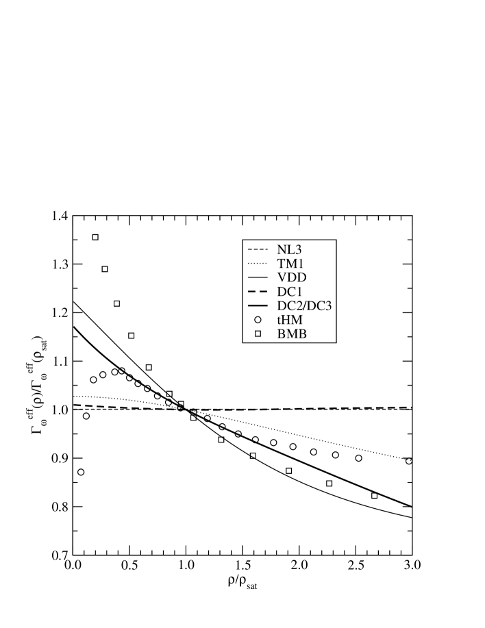
Figure 2: Normalized effective coupling constant of the $\omega$-meson in symmetric nuclear matter as a function of the normalized nucleon density in various relativistic mean field parametrizations and Dirac-Brueckner calulations.

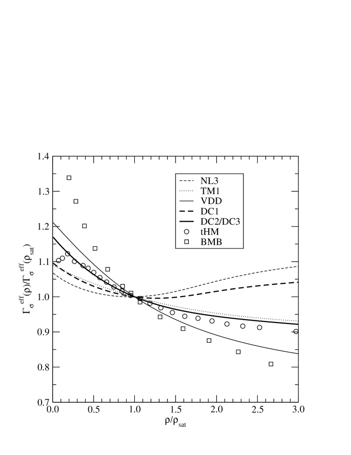
Figure 3: Normalized effective coupling constant of the $\sigma$-meson in symmetric nuclear matter as a function of the normalized nucleon density in various relativistic mean field parametrizations and Dirac-Brueckner calulations.

The TM1 parametrization achieves a slightly softer equation of state for symmetric nuclear matter at high densities than the NL3 and DC1 models, respectively, and the effective $\omega$ coupling decreases significantly with increasing density. In this model a quartic self-coupling of the $\omega$-meson are taken explicitly into account in the Lagrangian density. It gives rise to a $\omega_{0}^{3}$ contribution in the meson field equation that becomes important at high densities and consequently reduces the vector self-energy.

The VDD model shows an even softer equation of state at high densities as compared to the above parametrizations. This behaviour is determined by the functional form of the density dependence of the coupling functions, which was chosen in order to describe effective coupling constants extracted from Dirac-Brueckner calculations of nuclear matter. In Figures 2 und 3 the corresponding results of two DB calculations (BMB with Bonn B potential Bro90 , tHM tHM87 ) are shown for comparison. Here, the strong decrease of the couplings with the density is evident although there is a considerable difference between the DB calculations. The DC2 and DC3 models, which are only different with respect to their isovector properties, also exhibit a reduction of the effective couplings similar to the VDD parametrization and the DB results. The derivative couplings in the Lagrangian generate an energy and density dependence of the self energies that leads to a significant decrease of the effective couplings. Consequently, the binding energy per nucleon rises much slower with density than in the NL3, DC1 and TM1 parametrizations.

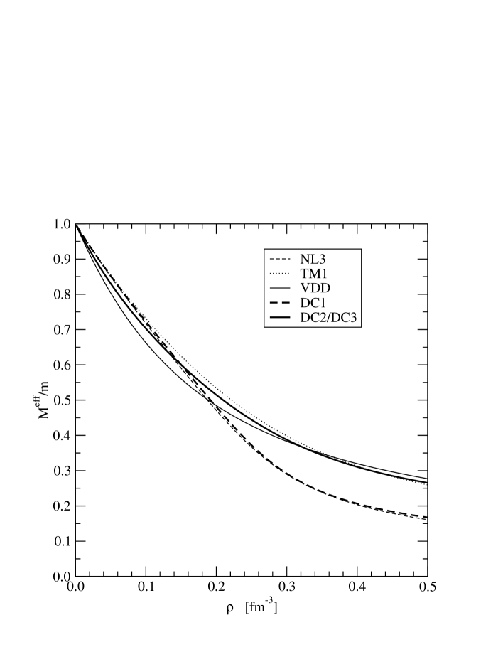
Figure 4: Relativistic effective nucleon mass in symmetric nuclear matter in units of the nucleon rest mass as a function of the nucleon density in various relativistic mean field parametrizations.

The density dependence of the effective $\sigma$-meson coupling and of the scalar self-energy is directly related to the decrease of the relativistic effective mass of the nucleon $M^{\rm eff}$ which is shown in Figure 4 for symmetric nuclear matter. We recall that the effective mass of the DC models is fixed to a value of $0.6$ at $\varrho_{\rm sat}$. There a two distinctly different groups, especially at high densities. The parametrizations NL3 and DC1 show a very similar behaviour as for the equation of state. The effective mass of these sets is substantially smaller than the mass of the other parametrizations at high densities and the curve exhibits less curvature. In symmetric nuclear matter the effective nucleon masses in the DC2 and DC3 model are identical but depend except on the density of the medium also on the momentum of the nucleon. In Figure 4 the effective mass of nucleons in the DC2/DC3 parametrizations is shown for the Fermi momentum $p^{F}$. The effective mass in the VDD model is smaller than in the other models at saturation density which is reflected by the too large spin-orbit splitting in finite nuclei Typ99 but the density dependence is more similar to the TM1, DC2 and DC3 cases.

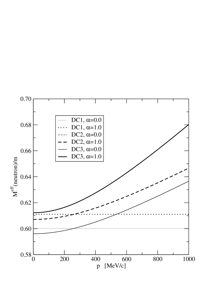
Figure 5: Momentum dependence of the neutron effective mass in units of the nucleon mass for the DC parametrizations in symmetric nuclear matter (thin lines) and neutron matter (thick lines) at $\varrho=0.150$ fm^-3. (The curves for $\alpha=0.0$ in the DC2 and DC3 model are identical.)

In Fig. 5 we show the momentum dependence of the neutron effective mass of different models for different asymmetries. The effective nucleon mass $M^{\rm eff}$ in the DC models is fixed to $0.6$ m at saturation density $\varrho_{\rm sat}=0.150$ fm^-3 for nucleons with the Fermi momentum in symmetric nuclear matter. The scalar self energy in the DC1 parametrization does not depend on the energy and therefore the effective mass is momentum independent. It increases only slightly with the neutron-proton asymmetry $\alpha$ at constant density. In the DC2 and DC3 models $M^{\rm eff}$ increases with the momentum and with the asymmetry. For $\alpha=0$ the effective mass is identical for DC2 and DC3 but in asymmetric nuclear matter the absolute value and the momentum dependence of $M^{\rm eff}$ are different. This effect is caused by the different values of $\Gamma_{\rho}$ and the non-zero $\Gamma_{\rho}^{(1)}$ in the DC3 case. The momentum dependence becomes stonger at higher densities.

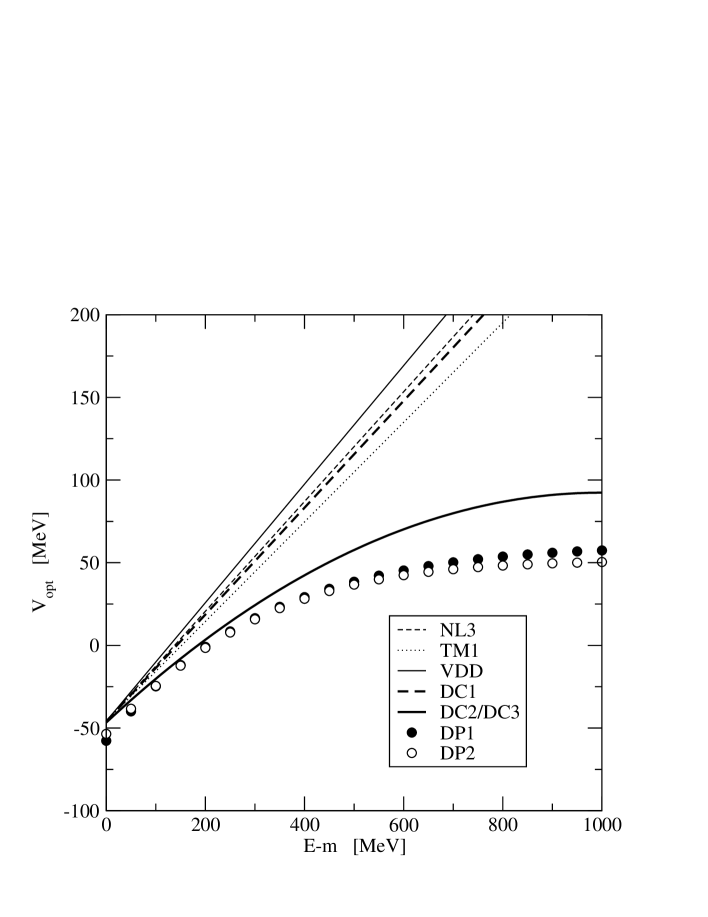
Figure 6: Dependence of the Schrödinger equivalent optical potential on the nucleon energy in symmetry nuclear matter at $\varrho=0.150$ fm^-3 in various relativistic mean field models and in two fits (DP1, DP2) of proton-nucleus scattering in Dirac phenomenology.

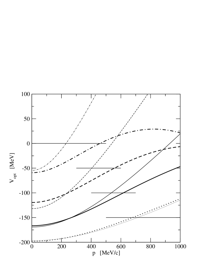
Figure 7: Dependence of the Schrödinger equivalent optical potential on the nucleon momentum in symmetric nuclear matter at various densities for the parametrizations DC1 (thin lines) and DC2/DC3 (thick lines). The potentials at $\varrho=0.5\varrho_{\rm sat}$ (dotted lines), $\varrho=1.0\varrho_{\rm sat}$ (solid lines), $\varrho=1.5\varrho_{\rm sat}$ (dashed lines), and $\varrho=2.0\varrho_{\rm sat}$ (dot-dashed lines) are shifted downwards by 150 MeV, 100 MeV, 50 MeV and 0 MeV, respectively. Horizontal lines mark the range in the momentum where the potential crosses zero.

The main difference between the DC2/DC3 parametrizations and the other models becomes apparent when the Schrödinger equivalent optical potential is studied, which is shown in Fig. 6 for $\varrho=\varrho_{\rm sat}$ as a function of the nucleon energy. In all models without energy dependent self-energies the optical potential by construction rises linearly with the energy in contrast to the real part of the optical potential extracted from Dirac phenomenology Ham90 ; Coo93 . This is clearly seen in Figure 6. At energies $E-m$ below approx. 200 MeV the optical potential is attractive. It higher energies it becomes repulsive. The linear increase of the RMF models leads to a substantial overestimate of the optical potential at energies above a few hundred MeV. Only the DC2 and DC3 models show a significant reduction of the repulsive potential at high energies, even though it is still larger than the experimental results from Dirac phenomenology. A fit of the parameters in the DC model with less constraints on the coupling constants than in the DC2/DC3 sets can certainly improve this agreement but one has to consider that the phenomenological scalar and vector potentials have an imaginary part which is absent in the DC model. Therefore, a comparison of the optical potentials at high energies has to viewed with caution. However, the DC model represents a significant qualitative improvement as compared to standard RMF models.

Figure 8: Dependence of the Schrödinger equivalent optical potential on the density in symmetric nuclear matter for the parametrizations DC1 (thin lines) and DC2/DC3 (thick lines) at nucleon momenta of $p=0$ MeV (dotted lines), $p=200$ MeV (solid lines), $p=400$ MeV (dashed lines), and $p=600$ MeV (dot-dashed lines).

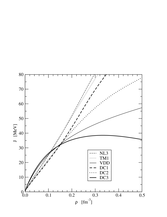
Figure 9: Dependence of the symmetry energy for symmetric nuclear matter on the nucleon density in various relativistic mean field parametrizations.

The DC models also makes a prediction on the momentum dependence of the optical potential at different medium densities. In Figure 7 the results of the parametrization DC1 are compared to the DC2/DC3 parametrizations at four nuclear matter densities between one half and twice the saturation density. The DC1 parameter set exhibits the typical behaviour of a RMF model with energy-independent self-energies. The optical potential rises fast with increasing nucleon momentum and becomes repulsive at progressively smaller momenta as the density of the medium increases. The DC2/DC3 models with momentum-dependent self-energies shows a similar trend as the DC1 model at small densities but at higher densities the optical potential is much less repulsive than in the DC1 model. The shift in the zero of $V_{\rm opt}$ is less pronounced and the nontrivial momentum dependence generates a considerable curvature. The density-dependence of the optical potential for constant nucleon momentum is shown in Fig. 8 and exhibits significant differences when the set DC1 is compared to the sets DC2/DC3. The optical potential vanishes at zero density independent of the nucleon momentum. It becomes smaller with increasing density and reaches a minimum before it rises again. The minimum is deeper for smaller momenta. At lower densities the parametrizations DC1 and DC2/DC3 display a more or less similar behaviour but at high densities the optical potential in the model without momentum dependent self-energies strongly increases and becomes very repulsive whereas the slope of $V_{\rm opt}$ in the other model is much smaller and the repulsion sets in much later.

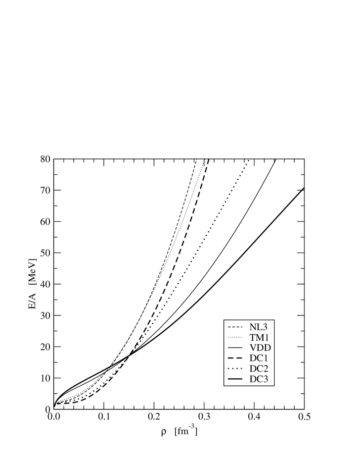
Figure 10: Binding energy per nucleon for neutron matter as a function of the neutron density in various relativistic mean field parametrizations.

The various parametrizations also exhibit a clearly distinct behaviour in the density dependence of the symmetry energy which is presented in Figure 9. The sets NL3, TM1, DC1, DC2 show an almost linear increase of $J$ over a large range of densities. In all these models the coupling of the nucleons to the $\rho$-meson is described by only one parameter, the constant $\Gamma_{\rho}$ of the minimal coupling. In the VDD model, the curve bends significantly with a smaller slope at saturation density because $\Gamma_{\rho}$ is a decreasing function with density. The effect is even larger in the DC3 parametrization where the symmetry energy derivative $L$ at saturation density was fitted to a smaller but more realistic value than in the other relativistic models. Comparing only the parametrizations NL3, TM1, and VDD, which were fitted to properties of finite nuclei, one notices that the symmetry energy at saturation density of the NL3 and TM1 models is much larger than in the VDD model but that $J$ is very similar around a density of $0.11$ fm^-3.

The density dependence of the symmetry energy directly correlates with the slope of the equation of state for neutron matter which is shown in Figure 10. The parametrizations NL3, TM1, DC1, and DC2 show a much stiffer equation of state than the density-dependent VDD model and the DC3 model with the smaller symmetry energy derivative $L$. The difference of the models is especially apparent at small densities. In Refs. Bro00 ; Typ01 it was shown that the slope of the neutron matter equation of state is directly correlated with the neutron skin thickness of finite nuclei, i.e. the difference between neutron and proton radii. This relation holds in both nonrelativistic Skyrme Hartree-Fock models and relativistic mean-field models. Experiments to determine neutron radii of finite nuclei with higher precision than available today can lead to better constraints on the model parameters and to better predictions for the neutron matter equation of state. It can be expected that the DC3 model with the smallest slope will also give a small neutron skin thickness similar to several Skyrme parametrizations when applied to calculations of finite nuclei.

V Summary and outlook

The DC model is an extension of standard relativistic quantum hadronic models in order to generate an effective momentum dependence of the self energies in the mean field approximation. This is achieved by introducing couplings of the meson fields to derivatives of the nucleon field in the Lagrangian density. The new contributions lead to additional source terms in the meson field equations and to a density dependence of the effective meson masses. The effective interaction in the DC model is both medium and state dependent. The self energies in the Dirac equation are differential operators with a nontrivial density dependence. The effective mass depends in general on the density, the momentum and the neutron-proton asymmetry.

We applied the DC model to nuclear matter and developed three parametrizations for the coupling constants under different conditions. The set DC1 without momentum dependent self energies is similar to previous nonlinear RMF models. It displays rather stiff equations of state for symmetric nuclear matter and neutron matter. The sets DC2 and DC3 lead to energy dependent self energies The equation of state becomes softer and is comparable to the RMF model with density dependent couplings. The Schrödinger equivalent optical potential is much less repulsive than in standard RMF parametrizations at high nucleon energies. It shows an energy dependence more like optical potentials extracted from Dirac phenomenology. The DC model is also flexible to adjust isovector properties which affects the neutron matter equation of state.

If the nucleon momenta are too large the assumption of a linear energy dependence of the self energies is no longer valid. In this case the DC model can no longer be applied. This deficiency could be improved by introducing couplings of the meson fields to higher derivatives of the nucleon fields. Since the medium density determines the Fermi momentum there is also a limitation of the model to not too large densities but the Fermi momentum increases only slowly with the density.

Because of the limited number of constraints from nuclear matter properties the parameter space of the DC model was not fully explored. It is worthwhile to apply the model to finite nuclei and to study the effects of the new coupling vertices in this case. Also important is the comparison to extensive experimental data on nucleon scattering. The parametrizations developed here can be used as a reasonable starting point for a further refinement.

The approach of the DC model with fixed coupling constants but generalized interaction vertices in the Lagrangian density is in the spirit of non-linear RMF models. Alternatively, one can think of an extension of models with density dependent meson-nucleon vertices by introducing a dependence of the coupling functions on derivative densities. We currently also investigate the possibilities of such an approach and results will be reported in the future.

Appendix A Explicit expressions of densities

The conserved current densities in the field equations of the $\omega$- and $\rho$-meson are given as

$$J_{\mu} = [(1+\mathcal{W})g_{\mu\nu}+\mathcal{X}_{\mu\nu}]j^{\nu}-\mathcal{T}_{\mu}\varrho_{s}+\vec{\mathcal{W}}\cdot\vec{\jmath}_{\mu}-\vec{\mathcal{T}}_{\mu}\cdot\vec{\varrho}_{s}$$ (75)

$$\vec{J}_{\mu} = [(1+\mathcal{W})g_{\mu\nu}+\mathcal{X}_{\mu\nu}]\vec{\jmath}^{\nu}-\mathcal{T}_{\mu}\vec{\varrho}_{s}$$

$$+\vec{\mathcal{W}}j_{\mu}-i\vec{\mathcal{W}}\times\vec{\jmath}_{\mu}-\vec{\mathcal{T}}_{\mu}\varrho_{s}+i\vec{\mathcal{T}}_{\mu}\times\vec{\varrho}_{s}$$

and depend on the usual scalar densities and vector densities. The derivative scalar densities

$$\varrho_{s}^{D} = \varrho_{s}^{d}-\Gamma_{\omega}\omega_{\mu}j^{\mu}-\Gamma_{\rho}\vec{\rho}_{\mu}\cdot\vec{\jmath}^{\mu}=g^{\mu\nu}t^{D}_{\mu\nu}$$ (77)

$$\vec{\varrho}_{s}^{D} = \vec{\varrho}_{s}^{d}-\Gamma_{\omega}\omega_{\mu}\vec{\jmath}^{\mu}-\Gamma_{\rho}\vec{\rho}_{\mu}j^{\mu}+i\Gamma_{\rho}\vec{\rho}_{\mu}\times\vec{\jmath}^{\mu}=g^{\mu\nu}\vec{t}^{D}_{\mu\nu}$$ (78)

with

$$\varrho_{s}^{d} = \frac{1}{2}\langle\left[\bar{\psi}\gamma^{\mu}i\partial_{\mu}\psi-(i\partial_{\mu}\bar{\psi})\gamma^{\mu}\psi\right]\rangle=g^{\mu\nu}t^{d}_{\mu\nu}$$ (79)

$$\vec{\varrho}_{s}^{d} = \frac{1}{2}\langle\left[\bar{\psi}\gamma^{\mu}i\partial_{\mu}\vec{\tau}\psi-(i\partial_{\mu}\bar{\psi})\gamma^{\mu}\vec{\tau}\psi\right]\rangle=g^{\mu\nu}\vec{t}^{d}_{\mu\nu}$$ (80)

are obtained from a contraction of the derivative tensor densities

$$t^{D}_{\mu\nu} = \frac{1}{2}\langle\left[\bar{\psi}\gamma_{\mu}iD_{\nu}\psi+\overline{(iD_{\nu}\psi)}\gamma_{\mu}\psi\right]\rangle=t^{d}_{\mu\nu}-\Gamma_{\omega}\omega_{\nu}j_{\mu}-\Gamma_{\rho}\vec{\rho}_{\nu}\cdot\vec{\jmath}_{\mu}$$ (81)

$$\vec{t}^{D}_{\mu\nu} = \frac{1}{2}\langle\left[\bar{\psi}\gamma_{\mu}iD_{\nu}\vec{\tau}\psi+\overline{(iD_{\nu}\psi)}\gamma_{\mu}\vec{\tau}\psi\right]\rangle=\vec{t}^{d}_{\mu\nu}-\Gamma_{\omega}\omega_{\nu}\vec{\jmath}_{\mu}-\Gamma_{\rho}\vec{\rho}_{\nu}j_{\mu}+i\Gamma_{\rho}\vec{\rho}_{\nu}\times\vec{\jmath}_{\mu}$$ (82)

where

$$t^{d}_{\mu\nu} = \frac{1}{2}\langle\left[\bar{\psi}\gamma_{\mu}i\partial_{\nu}\psi-(i\partial_{\nu}\bar{\psi})\gamma_{\mu}\psi\right]\rangle$$ (83)

$$\vec{t}^{d}_{\mu\nu} = \frac{1}{2}\langle\left[\bar{\psi}\gamma_{\mu}i\partial_{\nu}\vec{\tau}\psi-(i\partial_{\nu}\bar{\psi})\gamma_{\mu}\vec{\tau}\psi\right]\rangle$$ (84)

with the metric tensor $g^{\mu\nu}$. For the derivative current densities the expressions

$$j^{D}_{\mu} = j^{d}_{\mu}-\Gamma_{\omega}\omega_{\mu}\varrho_{s}-\Gamma_{\rho}\vec{\rho}_{\mu}\cdot\vec{\varrho}_{s}$$ (85)

$$\vec{\jmath}^{D}_{\mu} = \vec{j}^{d}_{\mu}-\Gamma_{\omega}\omega_{\mu}\vec{\varrho}_{s}-\Gamma_{\rho}\vec{\rho}_{\mu}\varrho_{s}+i\Gamma_{\rho}\vec{\rho}_{\mu}\times\vec{\varrho}_{s}$$ (86)

with

$$j^{d}_{\mu} = \frac{1}{2}\langle\left[\bar{\psi}i\partial_{\mu}\psi-(i\partial_{\mu}\bar{\psi})\psi\right]\rangle$$ (87)

$$\vec{j}^{d}_{\mu} = \frac{1}{2}\langle\left[\bar{\psi}i\partial_{\mu}\vec{\tau}\psi-(i\partial_{\mu}\bar{\psi})\vec{\tau}\psi\right]\rangle\>.$$ (88)

are found.

Appendix B Normalization of spinors

The spinors (45) in the solutions of the Dirac equation are normalized according to

$$\bar{u}(\vec{p},\sigma,\tau)\Gamma_{0\tau}u(\vec{p},\sigma^{\prime},\tau^{\prime})=\delta_{\sigma\sigma^{\prime}}\delta_{\tau\tau^{\prime}}$$ (89)

which guarantees that the zero component of the current density $J_{\mu}$ can be interpreted as the baryon density. Correspondingly, the relations

$$\bar{u}(\vec{p},\sigma,\tau)\gamma_{0}u(\vec{p},\sigma^{\prime},\tau^{\prime}) = \frac{\tilde{E}_{\tau}\delta_{\sigma\sigma^{\prime}}\delta_{\tau\tau^{\prime}}}{(1+W_{\tau}+X_{00\tau})\tilde{E}_{\tau}-T_{0\tau}\tilde{M}_{\tau}}$$

$$= \frac{\delta_{\sigma\sigma^{\prime}}\delta_{\tau\tau^{\prime}}}{(1+W_{\tau}+X_{00\tau})(1-B_{\tau}^{2})}\left(1+\frac{A_{\tau}B_{\tau}}{\sqrt{A_{\tau}^{2}+\tilde{p}_{\tau}^{2}}}\right)$$

and

$$\bar{u}(\vec{p},\sigma,\tau)u(\vec{p},\sigma^{\prime},\tau^{\prime}) = \frac{\tilde{M}_{\tau}\delta_{\sigma\sigma^{\prime}}\delta_{\tau\tau^{\prime}}}{(1+W_{\tau}+X_{00\tau})\tilde{E}_{\tau}-T_{0\tau}\tilde{M}_{\tau}}$$

$$= \frac{\delta_{\sigma\sigma^{\prime}}\delta_{\tau\tau^{\prime}}}{(1+W_{\tau}+X_{00\tau})(1-B_{\tau}^{2})}\left(B_{\tau}+\frac{A_{\tau}}{\sqrt{A_{\tau}^{2}+\tilde{p}_{\tau}^{2}}}\right)$$

for the usual scalar and vector densities are found. In the calculation of the scalar derivative density also the relation

$$\bar{u}(\vec{p},\sigma,\tau)\vec{\gamma}\cdot\vec{\tilde{p}}_{\tau}u(\vec{p},\sigma^{\prime},\tau^{\prime})=\frac{\vec{\tilde{p}}_{\tau}^{2}\delta_{\sigma\sigma^{\prime}}\delta_{\tau\tau^{\prime}}}{(1+W_{\tau}+X_{00\tau})\tilde{E}_{\tau}-T_{0\tau}\tilde{M}_{\tau}}$$ (92)

will be needed.

References

- (1) J. D. Walecka, Ann. Phys. (N.Y.) 83, 497 (1974).
- (2) P. Ring, Prog. Part. Nucl. Phys. 37, 193 (1996).
- (3) B. D. Serot and J. D. Walecka, Adv. Nucl. Phys. 16, 1 (1986); Int. J. Mod. Phys. E 6, 515 (1997).
- (4) B. D. Serot, Rep. Prog. Phys. 55, 1855 (1992).
- (5) Y. K. Gambhir, P. Ring, and A. Thimet, Ann. Phys. (N.Y.) 198, 132 (1990).
- (6) M. Rufa, P.-G. Reinhard, J. A. Maruhn, W. Greiner, and M. R. Strayer, Phys. Rev. C 38, 390 (1988).
- (7) P.-G. Reinhard, M. Rufa, J. Maruhn, W. Greiner, and J. Friedrich, Z. Phys. A 323, 13 (1986).
- (8) C. J. Horowitz and B. D. Serot, Nucl. Phys. A 368, 503 (1981).
- (9) S. A Chin, Ann. Phys. (N.Y.) 108, 301 (1977).
- (10) F. de Jong and H. Lenske, Phys. Rev. C 57, 3099 (1998).
- (11) L. Sehn, C. Fuchs, and A. Faessler, Phys. Rev. C 56, 216 (1997).
- (12) H. Huber, F. Weber, and M. K. Weigel, Phys. Rev. C 51, 1790 (1995).
- (13) H. F. Boersma and R. Malfliet, Phys. Rev. C 49, 233 (1994).
- (14) H. F. Boersma and R. Machleidt, Phys. Rev. C 49, 1495 (1994).
- (15) R. Fritz and H. Müther, Phys. Rev. C 49, 633 (1994).
- (16) G. Q. Li, R. Machleidt, and R. Brockmann, Phys. Rev. C 45, 2782 (1992).
- (17) F. de Jong and R. Malfliet, Phys. Rev. C 44, 998 (1991).
- (18) R. Brockmann and R. Machleidt, Phys. Rev. C 42, 1965 (1990).
- (19) W. Botermans and R. Malfliet, Phys. Rep. 198, 115 (1990).
- (20) H. Müther, R. Machleidt, and R. Brockmann, Phys. Lett. B 202, 483 (1988).
- (21) C. J. Horowitz and B. D. Serot, Nucl. Phys. A 464, 613 (1987).
- (22) B. ter Haar and R. Malfliet, Phys. Rep. 149, 207 (1987); Phys. Rev. C 36, 1611 (1987).
- (23) M. R. Anastasio, L. S. Celenza, W. S. Pong, and C. M. Shakin, Phys. Rep. 100, 327 (1983).
- (24) F. Hofmann, C. M. Keil, and H. Lenske, Phys. Rev. C 64, 034314 (2001)
- (25) S. Haddad and M. Weigel, Phys. Rev. C 48, 2740 (1993)
- (26) R. Brockmann and H. Toki, Phys. Rev. Lett. 68, 3408 (1992)
- (27) J. Boguta and A. R. Bodmer, Nucl. Phys. A 292, 413 (1977); J. Boguta, Phys. Lett. B 106, 250 (1981).
- (28) A. R. Bodmer, Nucl. Phys. A 526, 703 (1991).
- (29) G. A. Lalazissis, J. König, and P. Ring, Phys. Rev. C 55, 540 (1997).
- (30) Y. Sugahara and H. Toki, Nucl. Phys. A 579, 557 (1994).
- (31) M. M. Sharma, A. R. Farhan, and S. Mythili, Phys. Rev. C 61, 054306 (2000).
- (32) J. Zimanyi and S. A. Moszkowski, Phys. Rev. C 42, 1416 (1990).
- (33) P. Mitra, G. Gangopadyay, and B. Malakar, Phys. Rev. C 65, 034329 (2002).
- (34) Guo Hua, T. v. Chossy, and W. Stocker, Phys. Rev. C 61, 014307 (2000).
- (35) A. Delfino, C. T. Coelho, and M. Malheiro, Phys. Rev. C 51, 2188 (1994).
- (36) R. J. Furnstahl and B. D. Serot Nucl. Phys. A 671, 447 (2000).
- (37) R. J. Furnstahl, J. J. Rusnak, and B. D. Serot, Nucl. Phys. A 632, 607 (1998).
- (38) R. J. Furnstahl, B. D. Serot, and H. B. Tang, Nucl. Phys. A 615, 441 (1997).
- (39) M. Del Estal, M. Centelles, X. Viãnas, and S. K. Patra, Phys. Rev. C 63, 024314 (2001).
- (40) M. Del Estal, M. Centelles, and X. Viãnas, Nucl. Phys. A 650, 443 (1999).
- (41) H. Lenske and C. Fuchs, Phys. Lett. B345, 355 (1995).
- (42) C. Fuchs, H. Lenske, and H. H. Wolter, Phys. Rev. C 52, 3043 (1995).
- (43) S. Typel and H. H. Wolter, Nucl. Phys. A 656, 331 (1999).
- (44) T. Nikić, D. Vretenar, P. Finelli, and P. Ring, Phys. Rev. C 66, 024306 (2002).
- (45) S. Hama, B. C. Clark, E. D. Cooper, H. S. Sherif, and R. L. Mercer, Phys. Rev. C 41, 2737 (1990).
- (46) E. D. Cooper, S. Hama, B. C. Clark, and R. L. Mercer, Phys. Rev. C 47, 297 (1993).
- (47) S. Typel, O. Riedl, and H. H. Wolter, Nucl. Phys. A 709, 299 (2002).
- (48) P. Danielewicz, Nucl. Phys. A 673, 375 (2000).
- (49) C.-H. Lee, T. T. S. Kuo, G. Q. Li, and G. E. Brown, Phys. Lett. B 412, 235 (1997).
- (50) G. Q. Li and R. Machleidt, Phys. Rev. C 48, 2707 (1993).
- (51) T. Maruyama, W. Cassing, U. Model, S. Teis, and K. Weber, Nucl. Phys. A 573, 653 (1994)
- (52) K. Weber, B. Blättl, W. Cassing, H.-C. Dönges, A. Lang, T. Maruyama, and U. Mosel, Nucl. Phys. A 552, 571 (1993)
- (53) K. Weber, B. Blättl, W. Cassing, H.-C. Dönges, V. Koch, A. Lang, and U. Mosel, Nucl. Phys. A 539, 713 (1992)
- (54) D. Vretenar, T. Nikić, and P. Ring, Phys. Rev. C. 65, 024321 (2002).
- (55) N. M. Hugenholtz and L. van Hove, Physica 24, 363 (1958).
- (56) H. Feldmeier and J. Lindner, Z. Phys. A 341, 83 (1991).
- (57) C.-H. Lee, T. T. S. Kuo, C. Q. Li, and G. E. Brown, Phys. Rev. C 57, 3488 (1998).
- (58) B. C. Clark, E. D. Cooper, S. Hama, R. W. Finlay, and T. Adami, Phys. Lett. B 295, 189 (1993).
- (59) S. Typel and B. A. Brown, Phys. Rev. C 64, 027302 (2001).
- (60) B. A. Brown, Phys. Rev. Lett. 85, 5296 (2000).