Constraining the Leading Weak Axial Two-body Current by SNO and Super-K

Abstract

We analyze the Sudbury Neutrino Observatory (SNO) and Super-Kamiokande (SK) data on charged current (CC), neutral current (NC) and neutrino electron elastic scattering (ES) reactions to constrain the leading weak axial two-body current parameterized by $L_{1,A}.$ This two-body current is the dominant uncertainty of every low energy weak interaction deuteron breakup process, including SNO’s CC and NC reactions. Our method shows that the theoretical inputs to SNO’s determination of the CC and NC fluxes can be self-calibrated, be calibrated by SK, or be calibrated by reactor data. The only assumption made is that the total flux of active neutrinos has the standard ${}^{8}B$ spectral shape (but distortions in the electron neutrino spectrum are allowed). We show that SNO’s conclusion about the inconsistency of the no-flavor-conversion hypothesis does not contain significant theoretical uncertainty, and we determine the magnitude of the active solar neutrino flux.

I Introduction

Recent conclusive results from the Sudbury Neutrino Observatory (SNO) have established the existence of non-electron active neutrino components in the ${}^{8}B$ solar neutrino flux [1] and hence have given a strong evidence for neutrino oscillation. These results are based on the three reactions measured by SNO to detect the ${}^{8}B$ solar flux

$$\begin{array}[]{llll}\nu_{e}+d&\rightarrow&p+p+e^{-}&\qquad\text{(CC)},\\ \nu_{x}+d&\rightarrow&p+n+\nu_{x}&\qquad\text{(NC)},\\ \nu_{x}+e^{-}\!\!\!\!&\rightarrow&\nu_{x}+\text{{}}e^{-}&\qquad\text{(ES).}\end{array}$$ (1)

The charged current reaction (CC) is sensitive exclusively to electron-type neutrinos, while the neutral current reaction (NC) is equally sensitive to all active neutrino flavors ($x=e,\mu,\tau$). The elastic scattering reaction (ES) is sensitive to all active flavors as well, but with reduced sensitivity to $\nu_{\mu}$ and $\nu_{\tau}$. Detection of these three reactions allows SNO to determine the electron and non-electron active neutrino components of the solar flux, and it is then obvious that the cross sections for these three reactions are important inputs for SNO. The cross sections for all three reactions are determined from theory, but the CC and NC cross sections involve nuclear-physics complexities not present in the ES interaction description. Thus the CC and NC cross sections have become the main source of theoretical uncertainties for SNO.

The complexities in the CC and NC processes are due to two-body currents which are interactions involving two nucleons and external leptonic currents. In the potential model approach, the two-body currents are associated with the meson exchange currents and can be calculated in terms of unknown weak couplings. In effective field theory (EFT), the two-body currents are parameterized. In both cases, experimental data from some other processes are required in order to calibrate the unknowns in the problem. In EFT, this calibration procedure can be described in an economic and systematic way. The reason is that, up to next-to-next-to-leading order (NNLO) in EFT, all low-energy weak interaction deuteron breakup processes depend on a common isovector axial two-body current, parameterized by $L_{1,A}$ [2] (see more explanations in the next section). This implies that a measurement of any one of the breakup processes could be used to fix $L_{1,A}$. A summary of the previous efforts in the determination of $L_{1,A}$ can be found in Ref. [3].

In this paper, after briefly reviewing the EFT approach, we will present the constraint on $L_{1,A}$ using a combined analysis of the CC, NC and ES data from SNO and Super-Kamiokande (SK). We then compare this new result with other determinations of $L_{1,A}$ and comment on the interpretation of SNO’s measurements with the assumption about the size of $L_{1,A}$ eliminated.

II Effective Field Theory

For the deuteron breakup processes used to detect solar neutrinos, where the neutrino energies $E_{\nu}<15$ MeV, the typical momentum scales in the problem are much smaller than the pion mass $m_{\pi}(\simeq 140$ MeV$).$ In these systems pions do not need to be treated as dynamical particles since they only propagate over distances $\sim 1/m_{\pi}$, much shorter than the scale set by the typical momentum of the problem. Thus the pionless nuclear effective field theory, ${\rm EFT}({\pi\hskip-6.00006pt/})$ [4, 5, 6, 7, 8, 9], is applicable.

In ${\rm EFT}({\pi\hskip-6.00006pt/})$, the dynamical degrees of freedom are nucleons and non-hadronic external currents. Massive hadronic excitations such as pions and the delta resonance are not dynamical. Their contributions are encoded in the contact interactions between nucleons. Nucleon-nucleon interactions are calculated perturbatively with the small expansion parameter

$$Q\equiv\frac{\left(1/a,\gamma,p\right)}{\Lambda}$$ (2)

which is the ratio of the light to heavy scales. The light scales include the inverse S-wave nucleon-nucleon scattering length $1/a(\lesssim 12$ MeV$)$ in the ${}^{1}S_{0}$ channel, the deuteron binding momentum $\gamma(=45.7$ MeV) in the ${}^{3}S_{1}$ channel, and the typical nucleon momentum $p$ in the center-of-mass frame. The heavy scale $\Lambda$ is set by the pion mass $m_{\pi}$. This formalism has been applied successfully to many processes involving the deuteron [9, 10], including Compton scattering [11, 12], $np\rightarrow d\gamma$ for big-bang nucleosynthesis [13, 14], $\nu d$ reactions for SNO physics [2], the solar $pp$ fusion process [15, 16], and parity violating observables [17] . In addition, this formalism has been applied successfully to three-nucleon systems [18]. It has revealed highly non-trivial renormalizations associated with three body forces in the $s_{1/2}$ channel (e.g., ³He and the triton). For other channels, precision calculations were carried out to higher orders [8].

For low energy deuteron breakup processes, it is well known that the dominant contributions to the hadronic matrix elements are the ${}^{3}S_{1}\rightarrow$ ${}^{1}S_{0}$ transitions through the isovector axial couplings. The ${}^{3}S_{1}$ state (such as a deuteron) has spin $S=1$ and isospin $I=0$, while the ${}^{1}S_{0}$ state has $S=0$ and $I=1$. Amongst the spin-isospin operators 1, $\tau^{a}$, $\sigma^{i}$ and $\tau^{a}\sigma^{i}$, only the isovector axial coupling $\tau^{a}\sigma^{i}$ can connect ${}^{3}S_{1}$ to ${}^{1}S_{0}$ states. The ${}^{3}S_{1}\rightarrow\,^{3}S_{1}$ transitions are suppressed at low energies because i) the isovector operators do not contribute (the transition is isoscalar) and ii) the matrix elements of the one-body isoscalar operators vanish in the zero recoil limit ($d$ and $np$ states are orthogonal in this limit). This leads to large suppression of the isoscalar two-body contributions through the interference terms. Also, at low energies, the non-derivative operators are more important than the derivative operators. Thus the leading two-body current contributions for low energy weak interaction deuteron breakup processes only depend on a non-derivative, isovector axial two-body current, $L_{1,A}$.

In Ref. [2], ${\rm EFT}({\pi\hskip-6.00006pt/})$ is applied to compute the cross-sections for four channels (CC, NC, $\overline{\nu}_{e}+d\rightarrow e^{+}+n+n$ and $\overline{\nu}_{x}+d\rightarrow\overline{\nu}_{x}+n+p$) to NNLO, up to 20 MeV (anti)neutrino energies. As already mentioned, these processes have been shown to depend on only one parameter, $L_{1,A}$. This dependence is subject to an intrinsic uncertainty in our EFT calculation at NNLO of less than 3%. Through varying $L_{1,A}$, the potential model results of Refs. [20] and [21] are reproduced to high accuracy for all four channels. This confirms that the $\sim 5\%$ difference between Refs. [20] and [21] is due largely to different assumptions made about short distance physics.

The same two-body current $L_{1,A}$ also contributes to the proton-proton fusion process $p+p\rightarrow d+e^{+}+\nu_{e}$. This is the primary reaction in the $pp$ chain of nuclear reactions that power the sun, reactions which in turn generate the neutrino flux to be observed by SNO. The calculations in ${\rm EFT}({\pi\hskip-6.00006pt/})$ were carried out initially to second order [15], and then to fifth order [16]. Thus a calibration to SNO’s CC and NC reactions can also be used to calibrate the proton-proton fusion process.

III Fixing $L_{1,A}$ From a Combined NC, CC and ES Analysis

In this section we present the constraint on $L_{1,A}\$obtained from a combined analysis of the solar neutrino fluxes measured by CC, NC, and ES reactions. In SNO’s analysis, a specific $L_{1,A}\$was chosen in CC and NC reactions. The extracted solar neutrino fluxes from CC and NC were then compared to each other and to ES to extract a consistent set of neutrino flavor-conversion probabilities and to map allowed regions in a 2-mass mixing description. Here we take $L_{1,A}\$as a free parameter and use the available experimental data from SNO and SK to fix not only the flavor-conversion probabilities but also $L_{1,A}$. The only assumption we will make is that the total flux for the active solar neutrinos has the standard ⁸B shape.

In the two-flavor oscillation analysis there are three parameters extracted, $\Delta m_{12}^{2}$, $\theta_{12}$, and $\Phi_{\nu_{x}}$, which are the differences between the squares of the neutrino masses, the mixing angle, and the total active neutrino flux. There are three separate experimental inputs, the ES, CC, and NC rates. It might at first be thought impossible to extract a fourth parameter, $L_{1,A}$, without additional inputs or assumptions, such as fixing the shape of the electron-neutrino spectrum. The shape is experimentally determined, but not yet with high accuracy. Our strategy is to note that, in active-only oscillations, there is no shape distortion in the total flux, and that the integrated spectral response in the CC reaction over a certain range of final electron energies is the same as that in the ES reaction over a different range of energies, independent of distortions of the neutrino spectrum [23].

The CC and NC are measured at SNO and the ES is both measured at SNO and SK. The measured event rates are the integrals of the effective cross sections weighted by the solar neutrino fluxes that reached the target.

$$R_{NC} = \int dE\widetilde{\sigma}_{NC}f_{\nu_{x}}\ ,$$ (3)

$$R_{CC} = \int dE\widetilde{\sigma}_{CC}f_{\nu_{e}}\ ,$$ (4)

$$R_{ES} = \int dE\widetilde{\sigma}_{e}f_{\nu_{e}}+\int dE\widetilde{\sigma}_{\mu,\tau}\left[f_{\nu_{x}}-f_{\nu_{e}}\right]\ ,$$ (5)

where $R_{i}$ is the event rate, $f_{\nu_{i}}$ is the $\nu_{i}$ flux and $E$ is the neutrino energy. $\widetilde{\sigma}_{i}$ is the effective cross section, defined in Appendix A, with $i=e,\mu,\tau$ for $\nu_{e,\mu,\tau}+e$ ES interaction. These effective cross sections are the true cross sections convoluted with the detector resolution functions which describe how the energy is transferred to electrons and detected by their Cherenkov radiations. The effective cross sections depend on the electron detection threshold $T_{i}^{th}$. For CC and NC reactions, they also depend on $L_{1,A}$.

The total flux for the active solar neutrinos is assumed to have the standard ⁸B shape,

$$f_{\nu_{x}}\left(E\right)=\Phi_{\nu_{x}}\phi_{{}^{8}B}\left(E\right)\ ,$$ (6)

where $\phi_{{}^{8}B}$ is the normalized ${}^{8}B$ shape function ($\int_{0}^{E_{\max}}dE\phi_{8B}\left(E\right)=1$) [22] and $\Phi_{\nu_{x}}$ is the magnitude of the $\nu_{x}$ flux. This assumption is valid if there are no oscillations to sterile neutrinos, or, even if such mixing is present, the survival probability to active neutrinos is energy independent. Similarly, the $\nu_{e}$ flux is

$$f_{\nu_{e}}\left(E\right)=\Phi_{\nu_{x}}\phi_{{}^{8}B}\left(E\right)P_{\nu_{e}/\nu_{x}}\left(E\right)\ ,$$ (7)

where $P_{\nu_{e}/\nu_{x}}\left(E\right)$ is the probability distribution of finding a $\nu_{e}$ out of a $\nu_{x}$. Obviously, $P_{\nu_{e}/\nu_{x}}\left(E\right)$ is bounded between $0$ and $1$.

We follow Villante et al. in Ref.[23] to define the averaged effective cross sections $\overline{\sigma}_{i}$ and the normalized response functions $\rho_{i}\left(E\right)$ for the ${}^{8}B$ spectrum

$$\overline{\sigma}_{i} \equiv \int dE\widetilde{\sigma}_{i}\phi_{{}^{8}B}\left(E\right)\ ,$$ (8)

$$\rho_{i}\left(E\right) = \frac{\widetilde{\sigma}_{i}\phi_{{}^{8}B}\left(E\right)}{\displaystyle\int dE\widetilde{\sigma}_{i}\phi_{{}^{8}B}\left(E\right)}\ .$$ (9)

Then we rewrite eqs. (3-5) using eqs.(6-9)

$$R_{NC} = \Phi_{\nu_{x}}\overline{\sigma}_{NC}\ ,$$ (10)

$$R_{CC} = \Phi_{\nu_{x}}\overline{\sigma}_{CC}\int dE\rho_{CC}P_{\nu_{e}/\nu_{x}}\ ,$$ (11)

$$R_{ES} = \Phi_{\nu_{x}}\overline{\sigma}_{\mu,\tau}+\Phi_{\nu_{x}}\int dE\left[\overline{\sigma}_{e}\rho_{e}-\overline{\sigma}_{\mu,\tau}\rho_{\mu,\tau}\right]P_{\nu_{e}/\nu_{x}}\ .$$ (12)

An important observation made in Ref. [23] is that the terms with the normalized response function $\rho\left(E\right)$ dependence can be related by choosing suitable detection thresholds. This allows us to reduce the numbers of unknowns such that eqs.(10-12) become solvable. These approximate relations and their corrections are systematically explored in Appendix A. As shown in Fig.1(b), $\rho_{CC}$ is very insensitive to $L_{1,A}$. Thus we can set

$$\frac{\partial}{\partial L_{1,A}}\rho_{CC}\left(E\right)|_{T_{CC}^{th}=5\text{MeV}}=0\ .$$ (13)

Also, as shown in Fig. 1(c), to a very good approximation,

$$\rho_{e}\left(E\right)|_{T_{e}^{th}=6.8\text{MeV}}=\rho_{\mu,\tau}\left(E\right)|_{T_{\mu,\tau}^{th}=6.8\text{MeV}}\ .$$ (14)

The corrections of the above relations change $L_{1,A}$ by up to a negligible amount of 0.25 fm³. A more significant correction comes from

$$\rho\left(E\right)\equiv\rho_{CC}\left(E\right)|_{T_{CC}^{th}=5\text{MeV}}\cong\rho_{e}\left(E\right)|_{T_{e}^{th}=6.8\text{MeV}}\ .$$ (15)

We will use a parameter $\epsilon$ in eq.(22) to parametrize the correction.

Because of eq.(13), the $L_{1,A}$ dependence only shows up in $\overline{\sigma}_{NC}$ and $\overline{\sigma}_{CC}$. The scaling can be written as

$$\overline{\sigma}_{NC} = \overline{\sigma}_{NC}^{0}g_{NC}(L_{1,A})\ ,$$ (16)

$$\overline{\sigma}_{CC} = \overline{\sigma}_{CC}^{0}g_{CC}(L_{1,A})\ ,$$ (17)

where the $\overline{\sigma}_{NC}^{0}$ and $\overline{\sigma}_{CC}^{0}$ are the values used by SNO [1] which are based on the calculation of Ref. [24] with the electromagnetic radiative corrections of Ref. [25] (see Ref. [26] for an earlier attempt) and a 5 MeV electron detection threshold. These cross sections are corresponding to the NNLO EFT results with $L_{1,A}(\overline{\mu}=m_{\pi})=4.0$ fm³, where the renormalization scale $\overline{\mu}$ is set to the pion mass. In the following expressions, we will suppress the $\overline{\mu}$ dependence of $L_{1,A}$ for simplicity. The scaling functions can be parametrized as

$$g_{NC}(L_{1,A}) = 1+\alpha_{NC}\left(\frac{L_{1,A}}{\text{fm}^{3}}-4.0\right)\ ,$$ (18)

$$g_{CC}(L_{1,A}) = 1+\alpha_{CC}\left(\frac{L_{1,A}}{\text{fm}^{3}}-4.0\right)\ ,$$ (19)

where $\alpha_{NC}=0.013$ and $\alpha_{CC}=0.010$. It is interesting to note that if $\overline{\sigma}$ were averaged true cross sections instead of the averaged effective cross sections, then $\alpha_{NC}$ and $\alpha_{CC}$ would be almost identical [2]. The larger difference here is due to the difference in the detection methods. As shown in eqs.(A2) and (A5), the CC event detection requires the final state electron energy to be above a certain detection threshold, thus leptons transferring too much energy to the hadrons will not be detected. For NC detection, however, there is no such discrimination—all the neutrons generated in NC have the same probability to be detected in the thermalization and capture process. Thus in general, the scaling factor of NC is associated with that of more energetic scattering (with larger energy transfer to the hadrons) than that of CC. We find the qualitative difference between $\alpha_{NC}$ and $\alpha_{CC}$ is consistent with the neutrino energy dependence of the scaling factors calculated in Ref. [2].

Substituting eqs.(13-17) into the eqs. (10-12), we have

$$R_{NC} = \Phi_{\nu_{x}}\overline{\sigma}_{NC}^{0}g_{NC}(L_{1,A})\ ,$$ (20)

$$R_{CC} = \Phi_{\nu_{x}}\overline{\sigma}_{CC}^{0}g_{CC}(L_{1,A})\int dE\rho P_{\nu_{e}/\nu_{x}}\ ,$$ (21)

$$R_{ES} = \Phi_{\nu_{x}}\overline{\sigma}_{e}\left[\frac{\overline{\sigma}_{\mu,\tau}}{\overline{\sigma}_{e}}+\left(1-\frac{\overline{\sigma}_{\mu,\tau}}{\overline{\sigma}_{e}}\right)\left(1+\epsilon\right)\int dE\rho P_{\nu_{e}/\nu_{x}}\right]\ .$$ (22)

Note that $T_{CC}^{th}=T_{NC}^{th}=5$ MeV and $T_{\mu,\tau}^{th}=T_{e}^{th}=6.8$ MeV to be consistent with eq.(15 ). $\epsilon$ parametrizes the correction to the approximate identity of eq.(15). As shown in Appendix A , there is a model independent bound

$$\left|\epsilon\right|<4\%\ .$$ (23)

This correction introduces changes $L_{1,A}$ by up to $\pm 2.0\$fm³ but changes the other quantities by negligible amounts.

Now it is clear that eqs.(20-22) are solvable. The three equations determine three quantities: $\Phi_{\nu_{x}}$, $L_{1,A}$ and $\int dE\rho P_{\nu_{e}/\nu_{x}}$, which are the magnitude of the total active neutrino flux, the axial two-body current, and the measured $\nu_{e}/\nu_{x}$ ratio, respectively. If there is no neutrino oscillation, then $\int dE\rho P_{\nu_{e}/\nu_{x}}=1$.

For the experimental inputs, SNO has measured the ES rates, but the SK determination is more precise while in agreement with SNO. Therefore we use the SK measurements not only to provide a value for the integral above 6.8 MeV as shown above, but also to fix (and remove) the ES contribution to the total SNO rates above 5 MeV. With 1496 days of data, SK reports [27] the equivalent electron neutrino fluxes ($\equiv R_{ES}/\overline{\sigma}_{e}$) for analysis thresholds of 6.5 and 5.0 MeV,

$$\Phi_{{\rm SK}}(6.5) = \left(2.362_{-0.068}^{+0.074}\right)\times 10^{6}{\rm\ cm}^{-2}{\rm s}^{-1}\ ,$$ (24)

$$\Phi_{{\rm SK}}(5.0) = \left(2.348_{-0.066}^{+0.073}\right)\times 10^{6}{\rm\ cm}^{-2}{\rm s}^{-1}\ ,$$ (25)

respectively, where the statistical and systematic errors have been added in quadrature. Here and in the subsequent analysis in this paper, where asymmetric errors occur, we simply use the larger. We take the uncertainties in the two SK fluxes to be fully correlated. In view of the lack of significant threshold-energy dependence in the SK flux, we assume

$$\Phi_{{\rm SK}}(6.8)=\Phi_{{\rm SK}}(6.5)\ .$$ (26)

SNO provides a model-independent value for the NC rate, obtained by separating the CC and NC parts of the signal by their different radial and sun-angle dependences in the detector. This result is independent of the energy spectrum of the CC events. Converting the flux reported into an equivalent number of events gives $727\pm 190$ detected in the 306.4-day running period.

TABLE I.: Numbers of events reported by SNO for 306.4 live days for a kinetic energy threshold of 5 MeV. The uncertainties (except for the backgrounds) are statistical.

Reaction	Events	Uncertainty
Candidate Events	2928	54.1
Backgrounds	123	+21.6 -17.0
Total Neutrino Events	2805	+58.3 -56.7
ES (from SK)	258.3	8.0
Net NC + CC	2546.7	59
NC (CC shape unconstrained)	727	190
NC (CC shape constrained)	576.5	49.5

In Table I the event rates needed for the model-independent analysis are summarized. The “true” number of ES events in the SNO data set is derived from $\Phi_{{\rm SK}}(5.0)$ and the SNO effective elastic scattering cross section with a 5.0 MeV threshold ${\overline{\sigma}_{e}|}_{5.0}$,

$${\overline{\sigma}_{e}|}_{5.0}=1.10\times 10^{-4}\text{\ cm}^{2}\text{sT}^{-1}\ ,$$ (27)

derived from Ref. [1]. (The number is in excellent agreement with the $263.6\pm 26.4({\rm stat.})$ obtained during the SNO signal extraction.) One could derive a value for the CC rate directly from the fifth and sixth lines of this table, but the two would be highly correlated. It is preferable to make use of expressions for NC + CC and NC because the summed rate is essentially free of correlation with the NC rate. So we use

$$R_{NC}+R_{CC} = R_{tot}-\Phi_{{\rm SK}}(5.0){\overline{\sigma}_{e}|}_{5.0}{=}\left(2546\pm 59\right)\text{T}^{-1}\text{\ ,}$$ (28)

$$R_{NC} = \left(727\pm 190\right)\text{T}^{-1}\ ,$$ (29)

where T$=$306.4 days.

The averaged effective cross sections of SNO can be extracted from Ref. [1]

$$\overline{\sigma}_{NC}^{0} = 1.13\times 10^{-4}\text{\ cm}^{2}\text{sT}^{-1}\ ,$$ (30)

$$\overline{\sigma}_{CC}^{0} = 1.12\times 10^{-3}\text{\ cm}^{2}\text{sT}^{-1}\ .$$ (31)

The effective cross sections are subject to uncertainty from a variety of sources, tabulated by SNO [1]. These include principally the energy scale, vertex-reconstruction accuracy, and (for the NC reaction) energy resolution and neutron capture efficiency. The sources of uncertainty produce in some cases correlated variations in the effective cross sections, which are explicitly accounted for in the analysis.

In general we should have added $3\%$ systematics for the NNLO EFT calculations of $\overline{\sigma}_{NC}^{0}$ and $\overline{\sigma}_{CC}^{0}$, because for an EFT with a small expansion parameter $Q\sim 1/3$, 3% error is reasonable for a third order (NNLO) calculation. In the analysis of [2], however, a faster convergence is seen in four channels of (anti)neutrino-deuteron scattering, such that 1-2% higher corrections also seems reasonable. Furthermore, it is conceivable that the higher order corrections can be absorbed in $L_{1,A}$ in low energy processes. One indication that this might happen is in the comparison with the potential model calculations. The potential model results have quite different systematics to those of EFT. The fact that NNLO EFT can fit four channels of (anti)neutrino-deuteron reaction results of [21] to within $1\%$ [2] suggests that higher order effects can be absorbed in $L_{1,A}$. Further investigation is still required to see whether the higher order effects shift $L_{1,A}$ approximately the same amount. For matrix elements with similar kinematics, this is likely to be true. In our case, we have CC and NC in approximately the same energy region. Thus we expect the higher order effects just shift $L_{1,A}$ by a certain amount ($\sim+2$ to $+3$ fm³, with the sign fixed by the fifth order proton-proton fusion calculation [16, 3] as will be explained in more detail later) without introducing additional error to the $\Phi_{\nu_{x}}$ and $\int dE\rho P_{\nu_{e}/\nu_{x}}$ determinations.

For ES reactions with a $6.8$-MeV threshold, the ratio of the neutral current and electron neutrino scattering cross sections is,

$$\frac{\overline{\sigma}_{\mu,\tau}}{\overline{\sigma}_{e}}=0.153\ ,$$ (32)

with radiative corrections included.

Now we have all the inputs required to solve eqs. (20-22). The full set of equations is nonlinear in $L_{1,A}$, but a linearized solution may be obtained by making a first-order expansion for $g_{CC}/g_{NC}=1+(\alpha_{CC}-\alpha_{NC})(L_{1,A}/$fm${}^{3}-4.0)+\ldots$ The term quadratic in  $(L_{1,A}/$fm${}^{3}-4.0)$ is $\sim 10^{-4}$ and can be neglected. Using this approximation, the solutions of eqs.(20-21) are:

$$(\frac{L_{1,A}}{\text{fm}^{3}}-4.0)=\left[\alpha_{CC}\Phi_{{\rm SK}}(6.8)\overline{\sigma}_{CC}^{0}+(\alpha_{NC}-\alpha_{CC})R_{NC}\frac{\overline{\sigma}_{\mu\tau}}{\overline{\sigma}_{e}}\frac{\overline{\sigma}_{CC}^{0}}{\overline{\sigma}_{NC}^{0}}\right]^{-1}$$ (33)

$$\times\left\{\left[R_{tot}-\Phi_{{\rm SK}}(5.0){\overline{\sigma}_{e}|}_{5.0}-R_{NC}\right]\left(1-\frac{\overline{\sigma}_{\mu\tau}}{\overline{\sigma}_{e}}\right)(1+\epsilon)-\Phi_{{\rm SK}}(6.8){\overline{\sigma}_{CC}^{0}}+R_{NC}\frac{\overline{\sigma}_{\mu\tau}}{\overline{\sigma}_{e}}\frac{\overline{\sigma}_{CC}^{0}}{\overline{\sigma}_{NC}^{0}}\right\},$$ (34)

$$\int dE\rho P_{\nu_{e}/\nu_{x}}=\left(\Phi_{{\rm SK}}(6.8)\frac{g_{NC}\overline{\sigma}_{NC}^{0}}{R_{NC}}-\frac{\overline{\sigma}_{\mu,\tau}}{\overline{\sigma}_{e}}\right)\left(1-\frac{\overline{\sigma}_{\mu,\tau}}{\overline{\sigma}_{e}}\right)^{-1}\left(1+\epsilon\right)^{-1},$$ (35)

$$\Phi_{\nu_{x}}=\frac{R_{NC}}{g_{NC}\overline{\sigma}_{NC}^{0}}\ .$$ (36)

Inserting the experimental and theoretical quantities,

$$L_{1,A} = 4.0\pm 4.7(\rm stat.)\pm 4.5(\rm syst.)\ \text{fm}^{3}\ ,$$ (37)

$$\Phi_{\nu_{x}} = \left(6.4\pm 1.4\pm 0.6\right)\times 10^{6}\ \text{cm}^{-2}\text{s}^{-1}\ ,$$ (38)

$$\int dE\rho P_{\nu_{e}/\nu_{x}} = 0.25_{-0.07}^{+0.12}\pm 0.03\ .$$ (39)

The statistical errors in $L_{1,A}\$are dominated by $R_{NC}$, and the systematic errors by $\Phi_{\rm SK}$ and by vertex reconstruction accuracy in SNO.

TABLE II.: Determinations of the NNLO $L_{1,A}$ (at renormalization scale $m_{\pi}$) from different processes. The higher order theoretical systematics are expected to be absorbed by shifting $L_{1,A}$ by $\sim+2$ to $+3$ fm³ thus is not included in this table. Note that the CC, NC & ES combined analysis assumes the standard ${}^{8}B$ shape for the active neutrino flux. The tritium $\beta$ decay analysis assumes the three-body current is negligible. The helioseismology analysis does not include the uncertainties from the solar model. The last two entries are theoretical determinations. EFT dimensional analysis gives $\left|L_{1,A}\right|$ $\sim 6$ (fm³) which is denoted as $[-6,6]$ as its expected range.

Processes	$L_{1,A}$ (fm3)	References
CC, NC & ES	$4.0\pm 6.3$	[this work]
Reactor $\overline{\nu}$-$d$	$3.6\pm 4.6$	[3]
Tritium $\beta$ decay	$4.2\pm 0.1$	[29](see also [16, 3, 30])
Helioseismology	$4.8\pm 5.9$	[31]
Dimensional analysis	$\sim[-6,6]$	[2]
Potential model	$4.0$	[24]

A few comments can be made about the result we obtain in eq.(38). First, the only assumption we have made is that the active neutrino flux has the standard ${}^{8}B$ shape. The rest of the treatment is model independent in the sense that we have not assumed the size of $L_{1,A}$ or assumed any neutrino oscillation scenarios. Second, our result on $\int dE\rho P_{\nu_{e}/\nu_{x}}$ can be used to constrain neutrino oscillation parameters. Third, the size of the active neutrino flux is consistent with the $\nu_{e}$ flux of the standard solar model $\Phi_{SSM}=\left(5.05_{-0.81}^{+1.01}\right)\times 10^{6}\$cm^-2s^-1. This sets a constraint on the oscillations between the active and sterile neutrinos. Fourth, the range of $L_{1,A}$ we have obtained is consistent with the estimated value $\left|L_{1,A}\right|$ $\sim 6$ fm³ (at $\overline{\mu}=m_{\pi}$) from dimensional analysis [2]. It is also consistent with the constraints from reactor-antineutrino deuteron breakup processes [3] , tritium beta decay [29], helioseismology [31], and the latest improved potential model results [24] (corresponding to $L_{1,A}$ $=4.0$ fm³). The comparison of their corresponding NNLO $L_{1,A}$’s is listed in Table II. Here we have assumed that most of the higher order effects in EFT can be absorbed by $L_{1,A}$, and the higher order theoretical systematics are therefore not included in the assigned error bars. We expect a $+2$ to $+3$ fm³ contribution to the effective value of $L_{1,A}$ from higher orders. The sign is fixed by an explicit fifth-order calculation of the proton-proton fusion at threshold [16] which shows that $L_{1,A}$ shifts by +2 to +3 fm³ from the third order (NNLO) to the fifth order. Even though the tritium beta decay analysis assumes that the three-body current is negligible and the helioseismology analysis does not include the uncertainties from the solar model, it is still very encouraging that all the constraints agree with each other very well, given how different the physical systems are.

It is likely in the future the error bar of $R_{NC}$ could be reduced by a factor of 2. In that case, the error on $L_{1,A}\$ would be reduced to 5 fm³.

It is also interesting to reinvestigate the null hypothesis (specifically that all observed fluxes can be described consistently within the Standard Model of Particles and Fields) when $L_{1,A}\$ is allowed to float. $\int dE\rho P_{\nu_{e}/\nu_{x}}=1$ in the Standard Model, and thus the set of three equations (20-21) contain only two parameters. One finds that the set is inconsistent at 4.3 $\sigma$. Alternatively, if one uses the experimental determination of $L_{1,A}\$from reactor data (Table II), the null hypothesis fails at 5.1 $\sigma$ (SNO only) or 5.3 $\sigma$ (SNO and SK). Thus, even if SNO were to place no reliance at all on the theoretical calculations of short-distance physics [21, 24], it would still be true that the no-flavor-conversion hypothesis is ruled out with high confidence.

One might suspect that if the value of $L_{1,A}$ is taken from some other constraints, perhaps the ${}^{8}B$ shape assumption for the active neutrino flux can be removed. This question can be easily answered by inspecting the new set of equations

$$R_{NC} = \Phi_{B}\overline{\sigma}_{NC}^{0}g_{NC}\int dE\rho_{NC}P_{\nu_{e}\rightarrow\nu_{x}}\ ,$$ (40)

$$R_{CC} = \Phi_{B}\overline{\sigma}_{CC}^{0}g_{CC}\int dE\rho P_{\nu_{e}\rightarrow\nu_{e}}\ ,$$ (41)

$$R_{ES} = \Phi_{B}\overline{\sigma}_{e}\left[\frac{\overline{\sigma}_{\mu,\tau}}{\overline{\sigma}_{e}}\int dE\rho_{\mu,\tau}P_{\nu_{e}\rightarrow\nu_{x}}+\left(1-\frac{\overline{\sigma}_{\mu,\tau}}{\overline{\sigma}_{e}}\right)\left(1+\epsilon\right)\int dE\rho P_{\nu_{e}\rightarrow\nu_{e}}\right]\ ,$$ (42)

where

$\Phi_{B}$ are the un-oscillated ${}^{8}B$ $\nu_{e}$ flux and $P_{\nu_{e}\rightarrow\nu_{i}}$ is the probability distribution between the $\nu_{e}\rightarrow\nu_{i}$ transition. If $\rho_{NC}$ and $\rho_{\mu,\tau}$ satisfy the relation

$\displaystyle\rho_{NC}|_{T_{NC}^{th}=5\text{MeV}}=\rho_{\mu,\tau}|_{T_{\mu,\tau}^{th}=6.8\text{MeV}}\ ,$then one can determine $\int dE\rho_{NC}P_{\nu_{e}\rightarrow\nu_{x}}$, $\int dE\rho P_{\nu_{e}\rightarrow\nu_{e}}$ and $\Phi_{B}$ provided $L_{1,A}$ is given. Unfortunately, the above relation, which implies $\rho_{NC}|_{T_{NC}^{th}=5\text{MeV}}=\rho_{CC}|_{T_{CC}^{th}=5\text{MeV}}$, does not hold, as shown in Fig. 1(a) in Appendix A.

IV Conclusions

We have analyzed the SNO and SK data on CC, NC and ES reactions to constrain the leading axial two-body current $L_{1,A}.$ This two-body current contributes the biggest uncertainty in every low energy weak interaction deuteron breakup process, including SNO’s CC and NC reactions. The only assumption made in this analysis is that the total flux of active neutrinos has the standard ${}^{8}B$ spectral shape (but distortions in the electron neutrino spectrum are allowed). We have confirmed that SNO’s conclusions about the inconsistency of the no-flavor-conversion hypothesis and the magnitude of the active solar neutrino flux do not have significant theoretical model dependence. Our method has shown that SNO can be self-calibrated or be calibrated by SK with respect to theoretical uncertainties, and that the resulting calibration produces results in close accord with theoretical expectations. Alternatively, the purely experimental determination of $L_{1,A}\$from reactor antineutrino data can be used to remove the dependence on theory, and SNO’s conclusions are unaffected.

ACKNOWLEDGMENTS

We would like to thank Petr Vogel for useful discussions. JWC is supported, in part, by the Department of Energy under grant DOE/ER/40762-213. RGHR is supported by the DOE under Grant DE-FG03-97ER41020.

A Computation of the Normalized Response Functions to the ${}^{8}B$ Spectrum

In this Appendix, we define of the effective cross sections and then show the numerical results that support eqs.(13-15).

For CC and ES reaction, the effective cross section $\widetilde{\sigma}$ is related to the true cross section $\sigma$ through the relation

$$\widetilde{\sigma}_{CC(ES)}=\eta_{CC(ES)}\int_{T_{CC(ES)}^{th}}dT\int dT^{\prime}r_{CC(ES)}(T,T^{\prime})\frac{d\sigma_{CC(ES)}}{dT^{\prime}}\ ,$$ (A1)

where $\eta$ is an experimental efficiency, $T^{\prime}$ is the true kinetic energy of the final state lepton and $T$ is the electron energy recorded through the Cherenkov radiation of the electron, and $T^{th}$ is the detection threshold. If the resolution of the detector were perfect, the resolution function $r(T,T^{\prime})$ would be a delta function. For SNO, $r(T,T^{\prime})$ is a Gaussion function [1]

$$r_{CC(ES)}(T,T^{\prime})=\frac{1}{\sqrt{2\pi}\Delta_{CC(ES)}}\exp\left[-\frac{(T-T^{\prime})^{2}}{2\Delta_{CC(ES)}^{2}}\right]$$ (A2)

with resolution

$$\Delta_{CC}=\left(-0.0684+0.331\sqrt{\frac{T^{\prime}}{\text{MeV}}}+0.0425\frac{T^{\prime}}{\text{MeV}}\right)\text{MeV\ .}$$ (A3)

For ES reactions, we have used the SK result rather than the SNO result for better statistics. The resolution for SK is [23]

$$\Delta_{ES}=\sqrt{\frac{T^{\prime}}{10\text{MeV}}}1.5\text{MeV\ .}$$ (A4)

For NC reaction, the final state neutrons are thermalized then captured by deuterons to form tritons and photons in SNO’s first phase running. The photons subsequently excite electrons which produce Cherenkov radiation. Thus the SNO’s NC events can be recorded as electron detections as well. However, the kinematic information of the final state neutrons is lost in thermalization. Thus the resolution function is monoenergetic [32]

$$r_{NC}(T)=\frac{1}{\sqrt{2\pi}\Delta_{NC}}\exp\left[-\frac{(T-T_{NC})^{2}}{2\Delta_{NC}^{2}}\right]\ ,$$ (A5)

where $T_{NC}=5.08$ MeV and $\Delta_{NC}=1.11$ MeV. In contrast to eq.(A2), the effective NC differential cross section versus $E$ is not distorted

$$\widetilde{\sigma}_{NC}=\eta_{NC}\sigma_{NC}\int_{T_{NC}^{th}}dTr_{NC}(T)\ .$$ (A6)

We now turn to the computation of the normalized response functions of the ${}^{8}B$ spectrum define in eq.(9). In Fig. 1(a), $\rho_{CC}|_{T_{CC}^{th}=5\text{MeV}}$ (solid curve) and $\rho_{NC}|_{T_{NC}^{th}=5\text{MeV}}$ (dashed curve) are shown as functions of $E$. The two curves are quite different. $\rho_{NC}$ is independent of $T_{NC}^{th}$, according to eqs.(9) and (A6). In contrast, the peak of $\rho_{CC}$ can be shifted towards the high energy end by increasing $T_{CC}^{th}$. When $T_{CC}^{th}=5$MeV, $\rho_{CC}$ is close to a Gaussian function. Likewise, when $T_{e}^{th}=6.8$MeV, $\rho_{e}$ and $\rho_{\mu,\tau}$ are adjusted to be close to Gaussians as well. Thus $\rho_{CC}$, $\rho_{e}$ and $\rho_{\mu,\tau}$ can be related. To see how different they are, it is convenient to define the following functions,

$$\delta\rho_{CC} \equiv \rho_{CC}|_{L_{1,A}=5\ \text{fm}^{3}}-\rho_{CC}|_{L_{1,A}=0}\ ,$$ (A7)

$$\delta\rho_{e} \equiv \rho_{e}|_{T_{e}^{th}=6.8\text{MeV}}-\rho_{\mu,\tau}|_{T_{e}^{th}=6.8\text{MeV}}\ ,$$ (A8)

$$\delta\rho_{CC,ES} \equiv \rho_{CC}|_{T_{CC}^{th}=5MeV}-\rho_{e}|_{T_{e}^{th}=6.8\text{MeV}}\ .$$ (A9)

$\delta\rho_{CC}$, $\delta\rho_{e}$ and $\delta\rho_{CC,ES}$ are shown as functions of $E$ in Fig. 1 (b)-(d), respectively.

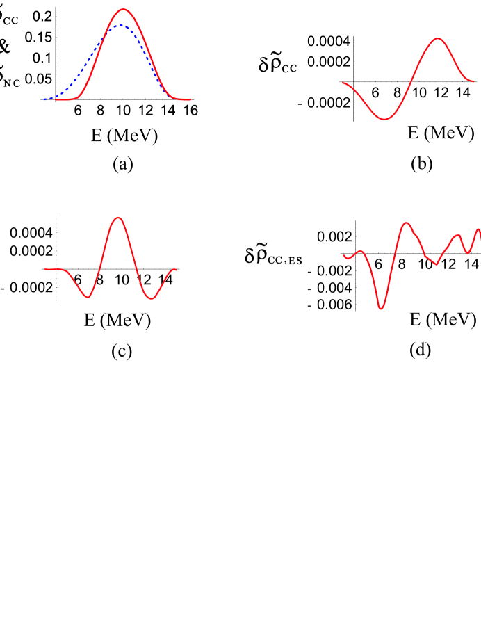
FIG. 1.: (a) $\rho_{CC}|_{T_{CC}^{th}=5\text{MeV}}$ (solid curve) and $\rho_{NC}|_{T_{NC}^{th}=5\text{MeV}}$ (dashed curve) are shown as functions of $E$. (b)-(d) $\delta\rho_{CC}$, $\delta\rho_{e}$ and $\delta\rho_{CC,ES}$ defined in eq.(A8) are shown as functions of $E$, respectively.

To study the contributions of non-zero $\delta\rho$, we will first prove an equality. Defining

$$\delta\rho_{\pm} = \frac{\delta\rho\pm\left|\delta\rho\right|}{2}\ ,$$ (A10)

$$I_{\pm} = \int dE\delta\rho_{\pm}P_{\nu_{e}/\nu_{x}}\ ,$$ (A11)

then

$$\int dE\delta\rho P_{\nu_{e}/\nu_{x}}=I_{+}+I_{-}\ .$$ (A12)

Since 0$\leq P_{\nu_{e}/\nu_{x}}\left(E\right)\leq 1$,

$$0 \leq I_{+}\leq\int dE\delta\rho_{+}\ ,$$ (A13)

$$\int dE\delta\rho_{-} \leq I_{-}\leq\ 0\ .$$ (A14)

Because $\int dE\delta\rho=0$, $\int dE\delta\rho_{\pm}=\pm\frac{1}{2}\int dE\left|\delta\rho\right|$. Thus we find

$$\left|\int dE\delta\rho P_{\nu_{e}/\nu_{x}}\right|\leq\frac{1}{2}\int dE\left|\delta\rho\right|\ .$$ (A15)

This model independent relation gives

$$\left|\int dE\delta\rho_{CC}P_{\nu_{e}/\nu_{x}}\right| \leq 0.0013\ ,$$ (A16)

$$\left|\int dE\delta\rho_{ES}P_{\nu_{e}/\nu_{x}}\right| \leq 0.0012\ ,$$ (A17)

$$\left|\int dE\delta\rho_{CC,ES}P_{\nu_{e}/\nu_{x}}\right| \leq 0.0105\ ,$$ (A18)

in comparison with $\int dE\rho P_{\nu_{e}/\nu_{x}}\sim 0.25$. The first two inequality show that the $L_{1,A}$ dependence in $\rho_{CC}$ and the difference between $\rho_{e}$ and $\rho_{\mu,\tau}$ are negligible compared with the correction from $\delta\rho_{CC,ES}$. The $\delta\rho_{CC,ES}$ effect is parametrized by $\epsilon$ in eq.(22) with

$$\left|\epsilon\right|<4\%\ .$$ (A19)

REFERENCES

- [1] Q.R. Ahmad et al., Phys. Rev. Lett. 87, 071301 (2001); Phys. Rev. Lett. 89, 011301 (2002), Phys. Rev. Lett. 89, 011302 (2002).
- [2] M.N. Butler and J.W. Chen, Nucl. Phys. A675, 575 (2000); M.N. Butler, J.W. Chen and X. Kong, Phys. Rev. C 63, 035501 (2001).
- [3] M.N. Butler, J.W. Chen, and Petr Vogel, nucl-th/0206026.
- [4] D.B. Kaplan, M.J. Savage and M.B. Wise, Nucl. Phys. B478, 629 (1996).
- [5] D.B. Kaplan, Nucl. Phys. B494, 471 (1997).
- [6] U. van Kolck, hep-ph/9711222; Nucl. Phys. A645 273 (1999).
- [7] T.D. Cohen, Phys. Rev. C55, 67 (1997); D.R. Phillips and T.D. Cohen, Phys. Lett. B390, 7 (1997); S.R. Beane, T.D. Cohen, and D.R. Phillips, Nucl. Phys. A632, 445 (1998).
- [8] P.F. Bedaque and U. van Kolck, Phys. Lett. B428, 221 (1998).
- [9] J.W. Chen, G. Rupak and M.J. Savage, Nucl. Phys. A653, 386 (1999).
- [10] J.W. Chen, G. Rupak and M.J. Savage, Phys. Lett. B464, 1 (1999).
- [11] S.R. Beane and M.J. Savage, Nucl. Phys. A694, 511 (2001).
- [12] H.W. Griesshammer and G. Rupak, Phys. Lett. B529, 57 (2002) .
- [13] J.W. Chen and M.J. Savage, Phys. Rev. C 60, 065205 (1999).
- [14] G. Rupak, Nucl. Phys. A678, 405 (2000).
- [15] X. Kong and F. Ravndal, Nucl. Phys. A656, 421 (1999); Nucl. Phys. A665, 137 (2000); Phys. Lett. B470 , 1 (1999); Phys. Rev. C 64, 044002 (2001).
- [16] M. Butler and J.W. Chen, Phys. Lett. B520, 87 (2001).
- [17] M.J. Savage, Nucl. Phys. A695, 365 (2001).
- [18] P.F. Bedaque, H.W. Hammer and U. van Kolck, Phys. Rev. Lett. 82, 463 (1999); Nucl. Phys. A 676, 357 (2000); H.-W. Hammer and T. Mehen, Phys. Lett. B 516, 353 (2001); P.F. Bedaque, G. Rupak, H.W. Griesshammer and H.W. Hammer, nucl-th/0207034.
- [19] P.F. Bedaque, H.-W. Hammer and U. van Kolck, Phys. Rev. C58, R641 (1998); F. Gabbiani, P.F. Bedaque and H.W. Grießhammer, Nucl. Phys. A 675, 601 (2000);
- [20] S. Ying, W.C. Haxton and E. M. Henley, Phys. Rev. C 45, 1982 (1992); Phys. Rev. D 40, 3211 (1989).
- [21] S. Nakamura, T. Sato, V. Gudkov and K. Kubodera, Phys. Rev. C 63, 034617 (2001).
- [22] C.E. Ortiz et al., Phys. Rev. Lett. 85, 2909 (2000); J.N. Bahcall et al., Phys. Rev. C 54, 411 (1996).
- [23] F.L. Villante, G. Fiorentini and E. Lisi, Phys. Rev. D59, 013006 (1998); G.L. Fogli, E. Lisi, A. Palazzo and F.L. Villante, Phys. Rev. D63, 113016 (2001).
- [24] S. Nakamura et al., Nucl. Phys. A707, 561 (2002).
- [25] A. Kurylov, M.J. Ramsey-Musolf and P. Vogel, Phys. Rev. C 65, 055501 (2002).
- [26] J.F. Beacom and S.J. Parke, Phys. Rev. D64, 091302 (2001).
- [27] S. Fukuda et al., Phys. Lett. B539, 179 (2002); Phys. Rev. Lett. 86, 5651 (2001).
- [28] E.K. Blaufuss, PhD Thesis, Louisiana State University, Dec 2000, http://www-sk.icrr.u-tokyo.ac.jp/doc/sk/pub/index.html.
- [29] R. Schiavilla et al., Phys. Rev. C 58, 1263 (1998).
- [30] T.S. Park et al., nucl-th/0106025; nucl-th/0208055; S. Ando et al., nucl-th/0206001.
- [31] K.I.T. Brown, M.N. Butler, and D.B. Guenther, nucl-th/0207008.
- [32] HOWTO use the SNO Solar Neutrino Spectral Data, SNO Collaboration, http://owl.phy.queensu.ca/sno/prlwebpage/.