Some remarks on the statistical model of heavy ion collisions

Abstract

This contribution is an attempt to assess what can be learned from the remarkable success of the statistical model in describing ratios of particle abundances in ultra-relativistic heavy ion collisions.

1 INTRODUCTION

As already pointed out in the contribution by A. Bialas [1] the statistical model (see e.g. [2]) works very well in describing/predicting measured ratios of particle abundances in ultra-relativistic heavy ion collisions. But even more remarkably, it works also for particle ratios measured in high energy proton-proton and even $e^{+}e^{-}$ collisions. In this contribution we will take the success of the statistical model as given and rather ask ourselves what can be learned from that. A critical discussion of possible shortcomings of the statistical model is given in the contribution of J. Rafelski [4].

In general a statistical description of a physical system is appropriate if the system has many degrees of freedom but is characterized only by few observables/measurements. This is e.g. the case in a thermal system, which is characterized only by the constants of motion, namely the energy (and momentum), volume and all the conserved particle numbers. (Of course in a canonical or grand canonical formulation, the energy and/or particles number are replaced by the conjugate variables temperature and chemical potential).

But not only a thermal system meets the requirements for a statistical description. Let us consider a high energy collision which produces many particles in the final state. If we are only interested in the number of pions produced, we constrain the final state very little, and thus statistical methods should be applicable. This is the idea of the statistical theory of particle production first invented by Fermi [5].

Now suppose the statistical model of Fermi applies for particle production in high energy collisions. Does that mean that we are dealing with a thermal system in the sense of Boltzmann, where particle collisions keep the system in a state of equilibrium? This is very unlikely in case of $e^{+}e^{-}$ collisions, where the produced particles hardly have a chance to re-interact. And actually explicit measurements [6] show no indication for interaction among the partons from different jets in $e^{+}e^{-}$ collisions (see also contribution by H. Satz [7]). Therefore, “statistical” does not always mean “thermodynamic” in the sense that one is dealing with matter in thermal equilibrium, and that one can define a pressure and an equation of state. Statistical may simply mean phase-space dominance and the ”temperatures” and ”chemical” potentials are nothing but Lagrange multipliers characterizing the phase-space integral [8, 9, 10]

This, however, may be different in a heavy ion collision. There one would naively expect (this is actually the main motivation for such complicated experiments) that the initially produced particles do re-interact on the partonic and/or hadronic level. The question then is, how to experimentally establish that a sufficient amount of re-interaction has taken place and that matter in the Boltzmann sense has been formed.

This contribution is organized as follows. In the first section, we will discuss the phase-space (or statistical model) for elementary collisions such as $e^{+}e^{-}$. Then we will proceed with nucleus-nucleus collisions. Finally we will try to assess to which extent a case for thermal matter can be made in nucleus-nucleus collisions. We will conclude with a discussion on what the statistical variables extracted from particle ratios can tell us about the phase structure of QCD.

2 PHASE-SPACE DOMINANCE

Let us consider a high energy collision of elementary particles such as $e^{+}e^{-}$ or proton proton. The probability to produce $n$ particles of a given species, such as pions, is given by

$$P_{n}=\sum_{x}P_{n,x}$$ (1)

where $P_{n,x}$ denotes the probability to find $n$ particles of interest and $x$ other particles in the final state,

$$P_{n,x}\sim\int\prod_{i=1}^{m}\frac{d^{3}q_{i}}{E_{i}}\left|M(q_{1},\ldots q_{m};\,p_{1},p_{2})\right|^{2}\delta(E-(\sum_{i=1}^{m}E_{i})\,\delta^{(3)}(\sum_{i=1}^{m}\vec{q}_{i}).$$ (2)

Here $E$ is the total energy of the system, which we consider in the center of momentum frame. The total multiplicity $m$ is given by

$$m=n+x.$$ (3)

In case of many particles in the final state, $m\gg 1$, one integrates over a large phase-space volume. As a result the details of the matrix element $M(q_{1},\ldots,q_{m};\,p_{1},p_{2})$ become less relevant. Instead one is sensitive to a phase-space average of the matrix element. Thus we can rewrite eq. (2) as

$$P_{n,x} \sim \left[\frac{1}{V^{m}}\left\langle\frac{\left|M(q_{1},\ldots,q_{m};\,p_{1},p_{2})\right|^{2}}{\prod_{i=1}^{m}E_{i}}\right\rangle\right]\,\,\,V^{m}\int\left(\prod_{i=1}^{m}d^{3}q_{i}\right)\delta(E-\sum_{i=1}^{m}E_{i})\,\delta^{(3)}(\sum_{i=1}^{m}\vec{q}_{i})$$ (4)

$$= \bar{S}_{m}\Phi_{m}(E)$$

where

$$\Phi_{m}(E)=V^{m}\int\left(\prod_{i=1}^{m}d^{3}q_{i}\right)\delta(E-\sum_{i=1}^{m}E_{i})\,\delta^{(3)}(\sum_{i=1}^{m}\vec{q}_{i})$$

is the micro-canonical m-particle phase-space volume known from statistical physics, and

$$\bar{S}_{m} = \left[\frac{1}{V^{m}}\left\langle\frac{\left|M(q_{1},\ldots,q_{m};\,p_{1},p_{2})\right|^{2}}{\prod_{i=1}^{m}E_{i}}\right\rangle\right]$$ (6)

$$= \frac{1}{\Phi_{m}(E)}\int\prod_{i=1}^{m}\frac{d^{3}q_{i}}{E_{i}}\left|M(q_{1},\ldots,q_{m};\,p_{1},p_{2})\right|^{2}\delta(E-\sum_{i=1}^{m}E_{i})\,\delta^{(3)}(\sum_{i=1}^{m}\vec{q}_{i})$$

denotes the phase-space averaged m-particle matrix element.

Obviously, if $\bar{S}_{m}$ is simply a constant, independent of $m$, and thus independent on $n$ and $x$, the relative probability to find a given number of particles is simply given by the ratio of the phase-space volumes,

$$\frac{P_{n}}{P_{n^{\prime}}}=\frac{\Phi_{n}(E)}{\Phi_{n^{\prime}}(E)},$$ (7)

or in other words, it is given by statistics only.

Similarly, the mean number of particles in this case is, up to a constant, given by statistics

$$\left\langle N\right\rangle=\sum_{n}nP_{n}\simeq\bar{S}\sum_{n,x}n\,\Phi_{n+x}(E),$$ (8)

where $\bar{S}$ denotes the constant averaged matrix element. Obviously, in this case particle ratios are given only by statistics, as the constant $\bar{S}$ drops out. Note, that for a large average multiplicity $\left\langle m\right\rangle=\left\langle n+x\right\rangle$, the sum in eq. (8) will be dominated by a few terms with $n+x\simeq\left\langle m\right\rangle$. This is analogous to the the grand-canonical approximation in statistical physics.

If the mean multiplicity is large, $\left\langle m\right\rangle\gg 1$, then the micro-canonical phase-space volume $\Phi_{m}(E)$ may be evaluated in the canonical or grand-canonical approximation [8, 9, 10] leading to Lagrange multipliers, which in the thermodynamic framework are the temperature and the chemical potential. In the situation at hand, however, these Lagrange multipliers do not have a physical meaning. They simply characterize the phase-space integral. Their actual magnitude depends on the available energy as well as on the density of states, i.e., the hadronic mass spectrum. They, however, do not reflect exchange of energy with a heat-bath, as is the case for the temperature in the canonical ensemble of thermal physics. Thus, in order to avoid confusion, we will denote the application of statistical physics in the non thermodynamics context by ”phase-space dominance”.

2.1 Conditions on the matrix elements

As discussed above, the essential assumption for phase-space dominance to work is that the phase-space averaged matrix elements (6) are constant, independent of $m$. What requirements does this impose on the matrix elements? Obviously, if the matrix elements simply scale with the multiplicity $m$ like

$$\left|M_{m}\right|^{2}=C\,\,(V^{m}\prod_{i=1}^{m}E_{i})$$ (9)

with $C$ being a constant, the condition is fulfilled. The scaling with $\prod_{i=1}^{m}E_{i}$ is simply due to the normalization of the states, and thus is not a dynamical constraint. The scaling with $V^{m}$ on the other hand is not trivial and implies that there is only one relevant length/mass scale in the problem. Before we discuss this in more detail let us list other conditions, which the matrix element has to satisfy.

• Absence of strong correlations. Correlations imply that the matrix element provides more support in localized regions of phase space. Consequently it is far from being constant. Or in other words, the integral in eq. (6) will only have support in a limited region leading to a decrease of $\bar{S}_{m}$ with increasing $m$.

• Absence of strong energy dependence in the matrix element. This is similar to the previous condition and actually related. Strong energy dependence (other than the trivial one from the normalization factors of the states) obviously implies a non-constant matrix element.

• Absence of strong interference effects, which lead to both correlations and energy dependencies.

Hadronic resonances, such as $\rho$ mesons give rise to correlations and energy dependencies. And indeed, the statistical model fails to reproduce the data if only true final state particles such as pions, kaons etc. are taken into account [11]. Instead, the successful fits of the particle ratios are obtained only if the hadronic resonances are part of the statistical ensemble. This way, the correlations are removed from the matrix elements and put into the ”final” states, in the spirit of [12]. This is schematically depicted in Fig.1.

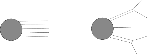
Figure 1: Resonances in the final state.

Thus, the relevant phase-space to be considered is a phase-space of all hadronic resonances and the matrix element is reduced to one with resonances in the final state

$$\Phi_{n}(E) \Rightarrow \Phi_{n^{\prime}}^{R}(E)$$

$$M(E;q_{1},\ldots,q_{m}) \Rightarrow M_{R}(E;p^{R}_{1},\ldots,p_{m^{\prime}}^{R})$$ (10)

As a result the reduced matrix element $M_{R}$ is free of all the correlations introduced by the resonances and, therefore, it is more likely that it meets the requirements stated above.

Let us return to the issue of the volume dependence of the matrix element. Only if the matrix element scales with the volume as given by eq. (9), the statistical approach is justified. From dimensional arguments an m-particle matrix element has the correct scaling behavior.

$$\frac{\left|M_{m}\right|^{2}}{E^{m}}\sim[{\rm mass}]^{-(3m+4)}.$$ (11)

In general there may be several length/mass scales contributing to the matrix element, such as e.g. the hadronic resonances. In this case the statistical approach should not work. If, on the other hand, all the dynamical mass scales of QCD aside from $\Lambda_{QCD}$ are the masses of the resonances, then the reduced matrix element $M_{R}$ (10) contains only $\Lambda_{\rm QCD}$, and the statistical approach will work as long as the volume is of the size of $1/\Lambda_{\rm QCD}^{3}$. This would be about the size of the proton, which appears to be a reasonable size for a volume in an elementary particle collision. We should note, however, that the fits to proton-proton collisions [13] lead to volumes of the order of $20\,\rm fm^{3}$, which is somewhat on the large side of what one would expect from our considerations here.

The constraints on the intrinsic mass scales, however, are not as severe as it might appear from the previous considerations. If the mean multiplicity $\left\langle m\right\rangle$ is large, the particle production is dominated by events with final state multiplicities near $\left\langle m\right\rangle$, i.e. $m=n+x$ is approximately constant for all n. And, therefore, the condition (9) is fulfilled trivially.

Finally, the matrix element is responsible for conservation laws due to intrinsic symmetries, such as strangeness, charge and baryon number. This, however, is already accommodated in the statistical approach. If the amount of conserved quanta is small, one may have to use a canonical description instead of a grand canonical one. But this is all within the framework of statistical physics, which actually is based on conservation laws.

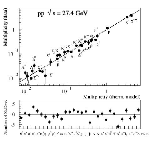
Figure 2: Fit of statistical model to particle ratio in proton-proton collisions (from [13]).

The success of the statistical fits to the particle ratios for $e^{+}e^{-}$ as well as proton proton is demonstrated in Fig. (2). As already pointed out, these fits are based on a statistical ensemble of hadronic resonances. Following the above arguments, we may conclude from the success of the statistical model that the relevant dynamical correlations and mass scales of QCD are contained in the hadronic resonances. In order to see more subtle dynamic effects, one probably has to resort to higher order correlations. The alternative conclusion would be that even in $e^{+}e^{-}$ collisions, re-scattering leads to a true thermodynamic system. This, however, is difficult to imagine and there is no experimental evidence for any re-scattering [6, 7].

Finally, let us point out that the statistical model also seems to work for correlation measurements of strange particles [13], such as $K_{s}\,K_{s}$. In the statistical approach, these correlations are mostly due to strangeness conservation and the agreement with the data indicates the absence of strong dynamical correlations.

3 NUCLEUS-NUCLEUS COLLISIONS

As we have discussed above, the success of the statistical model in describing particle yields in proton-proton collisions can be understood as a result of phase-space dominance. The goal of nucleus nucleus collisions, however, is to create matter, i.e., a thermal system in the sense of Boltzmann, where particle collisions lead to and maintain thermal equilibrium. It is only in this situation, where we can give the Lagrange multipliers ”$T$” and ”$\mu$” the physical meaning of temperature and chemical potential.

Obviously, if each individual nucleon-nucleon collision can be described by a statistical approach, we expect the statistical model to work even better in a nucleus-nucleus collision. And indeed it does, as can be seen from Fig.3. But how do we know that the statistical behavior of a nucleus-nucleus collision is again not simply phase-space dominance?

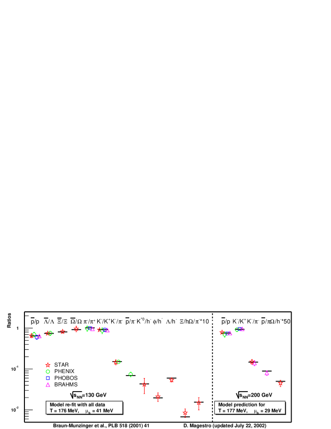
Figure 3: Fit of statistical model to particle ratio in Au+Au collisions at RHIC energies [14].

To illustrate this point, let us assume for a moment that a nucleus-nucleus collision is a simple superposition of “$N$” nucleon-nucleon collisions. Let us also assume that nucleon-nucleon collisions can be described by statistics as a result of phase-space dominance. If we were dealing with a simple classical ideal gas without additional constraints from conservation laws, the partition function of the nucleus-nucleus system $Z_{AA}$ is simply the product of the partition functions of the nucleon-nucleon collisions $Z_{nn}$

$$Z_{AA}^{(a)}=\prod_{i=1}^{N}Z_{nn}.$$ (12)

This situation is sketched in Fig.4a. There is no cross talk between the individual systems.

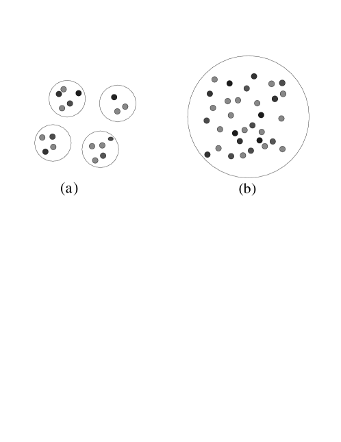
Figure 4: Individual nucleon-nucleon collisions (a) and nucleus-nucleus collision (b).

On the other hand $Z_{AA}^{(a)}$ also represents the partition function of a system of volume

$$V_{AA}=NV_{nn}$$ (13)

which would correspond to the system depicted in Fig.4b, and thus to “matter”, or in other words

$$Z_{AA}^{(a)}=Z_{AA}^{(b)}$$ (14)

So in this case there would be simply no way to distinguish between situation (a) and (b) in Fig.4 within a statistical framework.

So how can we find out if indeed thermalized matter has been created in a heavy ion collisions?

Obviously the factorization condition (14) will break down, once we probe the boundaries of phase-space available for a nucleon-nucleon collision, where the statistical model will not work. This could for example be achieved by studying $n$-particle correlations, with $n$ larger than the average multiplicity of a nucleon-nucleon collision, $n\gg\left\langle N\right\rangle_{nn}$. If, such a n-particle correlation would still look ”thermal” in an AA collision, then the vastly bigger phase space of an $AA$-system has been populated by scattering processes, and we may talk about “matter”.

The sensitivity of this approach can be improved by looking at conserved quantum numbers. If additional conservation laws, such as strangeness, are at work, phase space is even more restricted and factorization may break down already on the single particle level. Consider for example strangeness conservation. In scenario (a), strangeness has to be conserved for each nucleon-nucleon collision separately, whereas in (b) conservation applies only to the entire system. This additional constraint is most relevant if the number of strange particles produced in a nucleon-nucleon collision is small, $N_{s}\leq 1$. If $N_{s}\gg 1$ a grand-canonical treatment is adequate and factorization (14) works again at least on the single particle level. Consequently, in this case multi-particle correlations need to be investigated.

In nucleon-nucleon collisions a canonical treatment, where strangeness as well as baryon number are conserved explicitely, is required to explain the particle abundances [13, 16]. Also for lower energy and peripheral heavy ion collisions, the explicit treatment of strangeness conservation seems to required [17].

In [16] the centrality dependence of the strange baryon yields was studied based on the above concepts. The authors found, that the centrality dependence of the $\Omega$ enhancement should flatten out, once the volume over which strangeness is conserved exceeds that of about 20 time the volume of a nucleon. Therefore, if a flat centrality dependence of the $\Omega$ enhancement is observed, one can conclude that strangeness has ”percolated” at least over a volume 20 times as large as in a nucleon-nucleon collision. This would be a necessary but not sufficient condition for the existence of matter. Unfortunately the results reported by the NA57 collaboration [18] show a steep increase of the $\Omega$ enhancement up to the highest centralities.

However, even if the centrality dependence of the $\Omega$-enhancement is not completely understood, the fact that there is an $\Omega$-enhancement clearly shows that a nucleus-nucleus collision is more than simply a superposition of nucleon-nucleon collisions. And there is evidence from other observables that a certain amount of re-scattering is taking place in heavy ion collisions. Flow, radial or elliptic, would be difficult to understand without re-scattering on the partonic/hadronic level. To which extent they are sufficient to form matter in the Boltzmann sense is, however, not clear.

So have we formed matter in these collisions? A definitive answer to this question requires additional measurements such as multi-particle correlations of conserved quantities. At lower energy ($1-2\,\rm AGeV$) collisions, the measurement of kaon pairs for example provides a sensitive measurement on the degree of equilibrium reached [19]. At higher energies one might think about multiple $\Omega$ production, in order to really probe the boundaries of phase-space.

But we also have no evidence against the hypothesis of thermal equilibrium. Quite to the contrary, there is evidence for the necessary re-scattering from flow and dilepton production as well as $\Omega$-enhancement. Therefore, let us assume that we indeed have been able to create matter in these collision. In this case, we may interpret the Lagrange multipliers $T$ and $\mu$ as temperature and chemical potential. The result of fits to system at different collision energies [15, 17] is shown in Fig.5.

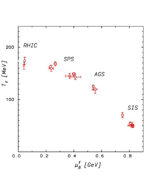
Figure 5: Results of thermal fits to particle ratios for different beam energies. Figure adapted from [17].

Does Fig.5 reflect a measurement of the phase-separation line in the QCD phase diagram? Certainly not! All it shows are the thermal parameters at which the systems fall out of chemical equilibrium under the assumption of unchanged particle properties. Does it tell us about a limiting temperature? Maybe! Suppose that LHC experiments lead to the same temperature of $T\simeq 170\,\rm MeV$. If at the same time radial flow increases considerably above the values observed at RHIC, then we can conclude that indeed much more energy has been deposited into the initial partonic system than reflected by the final temperature. Otherwise, one could argue that the constant temperature simply reflects the decreasing efficiency of depositing energy in the central rapidity region. Actually the radial flow from RHIC seems to be slightly larger than that extracted at the SPS [20, 21].

4 CONCLUSIONS

We have discussed the phase-space dominance assumption in the context of particle production in nucleon-nucleon, $e^{+}e^{-}$ and nucleus-nucleus collisions. The fact that the statistical model is able to explain observed particle ratios in these experiments may simply be a result of this assumption. We also have attempted to assess the difference between nucleus-nucleus and nucleon-nucleon collisions, and to which extent matter is produced in the former. While there is evidence for re-scattering processes to take place, we have not yet definitively established that a thermal system has been created in these collisions. A detailed study of multi-particle correlations of conserved quanta is one possible way to address this issue. Finally, we have argued that even if we consider the parameters extracted from the fits to the statistical model as temperature and chemical potential, the energy dependence of these parameters is not a measurement of the phase separation line of QCD.

5 ACKNOWLEDGMENTS

I would like to thank F. Becattini, P. Braun-Munzinger, J. Knoll, A. Majumder, J. Randrup, K. Redlich and S. Soff for useful discussions. This work was supported by GSI Darmstadt, and the Director, Office of Science, Office of High Energy and Nuclear Physics, Division of Nuclear Physics, and by the Office of Basic Energy Sciences, Division of Nuclear Sciences, of the U.S. Department of Energy under Contract No. DE-AC03-76SF00098.

References

- [1] A. Bialas, these proceedings.
- [2] F. Becattini, M. Gazdzicki and J. Sollfrank, Eur. Phys. Jour. C5, (1998) 143; P. Braun-Munzinger, I. Heppe and J. Stachel, Phys.Lett. B465 (1999) 15; F. Becattini, J. Cleymans, A. Keranen, E. Suhonen and K. Redlich, Phys. Rev. C64 (2001) 024901.
- [3] P. Braun-Munzinger, D. Magestro, K. Redlich and J. Stachel,Phys. Lett. B518 (2001) 41.
- [4] J. Rafelski, these proceedings.
- [5] E. Fermi, Progr. Theoret. Phys. 5 (1950) 570.
- [6] P. Abreu, hep-ph/0111395.
- [7] H. Satz, these proceedings.
- [8] R. Hagedorn, Relativistic Kinematics, W.A. Benjamin, New York, 1963.
- [9] E. Byckling and K. Kajantie, Particle kinematics, Wiley ,New York (1973).
- [10] L. Landau and L. Lifshitz, Statistical Physics, Pergamon Press, New York, 1980.
- [11] F. Becattini, private communication.
- [12] G.F. Uhlenbeck and E. Beth, Physica III (1936) 729.
- [13] F. Becattini and U. W. Heinz, Z. Phys. C76 (1997) 269.
- [14] Figure is most recent update of result published in [3]. Courtesy of P. Braun-Munzinger.
- [15] P. Braun-Munzinger and J. Stachel, Nucl.Phys. A606 (1996) 320.
- [16] S. Hamieh, K. Redlich and A. Tounsi, Phys. Lett. B486 (2000) 61
- [17] J. Cleymans and K. Redlich, Phys. Rev. C60 (1999) 054908
- [18] V. Manzari for the NA57 collaboration, these proceedings.
- [19] S. Jeon, V. Koch, K. Redlich and X. N. Wang, Nucl. Phys. A697 (2002) 546
- [20] N. Xu and M. Kaneta, Nucl. Phys. A698 (2002) 306c.
- [21] J.M. Burward-Hoy, for the PHENIX Collaboration, these proceedings.