Energy Density Functional Approach to Superfluid Nuclei

Abstract

We show that within the framework of a simple local nuclear energy density functional (EDF), one can describe accurately the one– and two–nucleon separation energies of semi–magic nuclei. While for the normal part of the EDF we use previously suggested parameterizations, for the superfluid part of the EDF we use the simplest possible local form compatible with known nuclear symmetries.

A steady transition is taking place during the last several years from the mean–field description of nuclear properties in terms of effective forces to an energy density functional approach (EDF). A significant role is played in this transition process by the fact that an EDF approach has a strong theoretical underpinning [1]. The effective forces used to derive the EDF are nothing else but a vehicle, since in themselves they have no well–defined physical meaning. For example, the effective Skyrme two–particle interaction is neither a particle–hole nor a particle–particle interaction. The particle–hole interaction (or the Landau parameters) is defined only as the second order functional derivative of the total EDF with respect to various densities, while the particle–particle interaction responsible for the pairing correlations in nuclei has to be supplied independently and with no logical connection to the Skyrme parameters.

We shall not attempt to even mention various mean–field approaches suggested so far, in this respect see Refs. [2], but we shall concentrate instead on a single aspect of the nuclear EDF, namely its pairing properties. Only recently it became clear that a theoretically consistent local EDF formulation of the nuclear pairing properties is indeed possible [3, 4, 5]. Even though the crucial role of the pairing phenomena in nuclei has been established firmly, it is surprising to realize how poor the quality of our knowledge still is. Phenomenologically, one cannot unambiguously decide whether the pairing correlations in nuclei have a volume or/and a surface character [6, 7, 8, 9, 10, 11, 12, 13]. The isospin character of the nuclear pairing correlations requires further clarification as well. These questions become even sharper in the language of a local EDF.

There is also the largely practical issue of whether one should use a zero–range or a finite–range effective pairing interaction. The only reason for the introduction of a finite–range was to resolve the formal difficulty with divergences in calculating the anomalous densities [10]. The majority of practitioners favor a much simpler approach, which embodies essentially the same physics, the introduction of an explicit energy cut–off. The best example are perhaps the works of the group [11, 12], which so far is the leader in describing all known nuclear masses. An explicit finite–range of the pairing interaction $r_{0}$ (which can be translated into an energy cut–off $E_{c}\approx\hbar^{2}/mr_{0}^{2}$) and a zero–range with an explicit energy cut–off $E_{c}$ in the final analysis are equivalent. Both approaches, however, are a poor’s man solution to the renormalization problem and reflect simply a lack of understanding of the role of high–momenta in the pairing channel. Neither the energy cut–off $E_{c}$ nor the finite–range of the interaction $r_{0}$ carry any physical information and they are simply means towards getting rid of infinities. The argument that nuclear forces have a finite–range is superfluous, see Refs. [3, 4, 5], since nuclear pairing phenomena are manifest at small energies and distances of the order of the coherence length, which is larger than nuclear radii.

We shall consider local nuclear EDFs only (which depend on various densities, as opposed to an explicit dependence on the full density matrix), as they proved overwhelmingly successful in describing normal nuclear properties. It is natural to expect that the same should apply to pairing properties. According to the general theorem of Hohenberg and Kohn [1] for many fermion systems there exists a universal EDF. Unfortunately there are no hints on how to derive such a functional. In the case of nucleons such a functional should satisfy some general constraints: rotational invariance, isospin invariance, time–reversal invariance and conservation of parity. Isospin symmetry is broken by Coulomb interaction, proton–neutron mass difference and charge symmetry breaking forces, the last two leading to rather small effects [13, 14]. In the case of Coulomb interaction mainly the direct term has to be accounted for, as the exchange and correlation Coulomb energies seem to cancel each other to some extent and their combined effect together with the effect of charge symmetry breaking forces is relatively small and responsible mainly for such rather subtle effects as the Nolen–Schiffer anomaly [13, 14]. We shall not consider here the contributions due to Coulomb exchange and charge symmetry breaking energies [14]. Such a structure of the normal nuclear EDF ${\cal{E}}_{N}(\mathchoice{{\hbox{\boldmath$\displaystyle r$}}}{{\hbox{\boldmath$\textstyle r$}}}{{\hbox{\boldmath$\scriptstyle r$}}}{{\hbox{\boldmath$\scriptscriptstyle r$}}})$ would be complete in the absence of superfluidity. Since pairing correlations in nuclear systems are known to be of rather small amplitude, we shall consider only a superfluid EDF ${\cal{E}}_{S}(\mathchoice{{\hbox{\boldmath$\displaystyle r$}}}{{\hbox{\boldmath$\textstyle r$}}}{{\hbox{\boldmath$\scriptstyle r$}}}{{\hbox{\boldmath$\scriptscriptstyle r$}}})$ of the following structure:

$${\cal{E}}_{S}(\mathchoice{{\hbox{\boldmath$\displaystyle r$}}}{{\hbox{\boldmath$\textstyle r$}}}{{\hbox{\boldmath$\scriptstyle r$}}}{{\hbox{\boldmath$\scriptscriptstyle r$}}})=g_{0}(\mathchoice{{\hbox{\boldmath$\displaystyle r$}}}{{\hbox{\boldmath$\textstyle r$}}}{{\hbox{\boldmath$\scriptstyle r$}}}{{\hbox{\boldmath$\scriptscriptstyle r$}}})|\nu_{p}(\mathchoice{{\hbox{\boldmath$\displaystyle r$}}}{{\hbox{\boldmath$\textstyle r$}}}{{\hbox{\boldmath$\scriptstyle r$}}}{{\hbox{\boldmath$\scriptscriptstyle r$}}})+\nu_{n}(\mathchoice{{\hbox{\boldmath$\displaystyle r$}}}{{\hbox{\boldmath$\textstyle r$}}}{{\hbox{\boldmath$\scriptstyle r$}}}{{\hbox{\boldmath$\scriptscriptstyle r$}}})|^{2}+g_{1}(\mathchoice{{\hbox{\boldmath$\displaystyle r$}}}{{\hbox{\boldmath$\textstyle r$}}}{{\hbox{\boldmath$\scriptstyle r$}}}{{\hbox{\boldmath$\scriptscriptstyle r$}}})|\nu_{p}(\mathchoice{{\hbox{\boldmath$\displaystyle r$}}}{{\hbox{\boldmath$\textstyle r$}}}{{\hbox{\boldmath$\scriptstyle r$}}}{{\hbox{\boldmath$\scriptscriptstyle r$}}})-\nu_{n}(\mathchoice{{\hbox{\boldmath$\displaystyle r$}}}{{\hbox{\boldmath$\textstyle r$}}}{{\hbox{\boldmath$\scriptstyle r$}}}{{\hbox{\boldmath$\scriptscriptstyle r$}}})|^{2},$$

where $\nu_{p,n}(\mathchoice{{\hbox{\boldmath$\displaystyle r$}}}{{\hbox{\boldmath$\textstyle r$}}}{{\hbox{\boldmath$\scriptstyle r$}}}{{\hbox{\boldmath$\scriptscriptstyle r$}}})$ are the $S=0$ proton/neutron anomalous densities. There is no firm evidence of pairing in other partial waves except the BCS–like $s$–wave in either proton or neutron channels and the evidence for neutron–proton pairing is inconclusive so far. Notice that ${\cal{E}}_{S}(\mathchoice{{\hbox{\boldmath$\displaystyle r$}}}{{\hbox{\boldmath$\textstyle r$}}}{{\hbox{\boldmath$\scriptstyle r$}}}{{\hbox{\boldmath$\scriptscriptstyle r$}}})$ is symmetric under the proton–neutron exchange. We assume that the effective couplings $g_{0,1}(\mathchoice{{\hbox{\boldmath$\displaystyle r$}}}{{\hbox{\boldmath$\textstyle r$}}}{{\hbox{\boldmath$\scriptstyle r$}}}{{\hbox{\boldmath$\scriptscriptstyle r$}}})$ might depend on position through the normal densities and that this dependence is consistent with expected symmetries. The density dependence of the effective couplings $g_{0,1}(\mathchoice{{\hbox{\boldmath$\displaystyle r$}}}{{\hbox{\boldmath$\textstyle r$}}}{{\hbox{\boldmath$\scriptstyle r$}}}{{\hbox{\boldmath$\scriptscriptstyle r$}}})$ arises from two different sources. Firstly, the bare coupling constant in the pairing channel could in principle have some intrinsic density dependence and such dependence has been considered by various authors during the years [2, 6, 7, 8, 9, 13]. Secondly, the renormalization of the pairing interaction, as described in our recent work [3, 4, 5], leads to position dependence as well. The equations for the quasi–particle wave functions $u_{i}(\mathchoice{{\hbox{\boldmath$\displaystyle r$}}}{{\hbox{\boldmath$\textstyle r$}}}{{\hbox{\boldmath$\scriptstyle r$}}}{{\hbox{\boldmath$\scriptscriptstyle r$}}})$ and $v_{i}(\mathchoice{{\hbox{\boldmath$\displaystyle r$}}}{{\hbox{\boldmath$\textstyle r$}}}{{\hbox{\boldmath$\scriptstyle r$}}}{{\hbox{\boldmath$\scriptscriptstyle r$}}})$ and related quantities are

$$E_{gs}=\int d^{3}r[{\mathcal{E}}_{N}(\mathchoice{{\hbox{\boldmath$\displaystyle r$}}}{{\hbox{\boldmath$\textstyle r$}}}{{\hbox{\boldmath$\scriptstyle r$}}}{{\hbox{\boldmath$\scriptscriptstyle r$}}})+{\mathcal{E}}_{S}(\mathchoice{{\hbox{\boldmath$\displaystyle r$}}}{{\hbox{\boldmath$\textstyle r$}}}{{\hbox{\boldmath$\scriptstyle r$}}}{{\hbox{\boldmath$\scriptscriptstyle r$}}})],$$ (1)

$${\mathcal{E}}_{S}(\mathchoice{{\hbox{\boldmath$\displaystyle r$}}}{{\hbox{\boldmath$\textstyle r$}}}{{\hbox{\boldmath$\scriptstyle r$}}}{{\hbox{\boldmath$\scriptscriptstyle r$}}}):=-\Delta(\mathchoice{{\hbox{\boldmath$\displaystyle r$}}}{{\hbox{\boldmath$\textstyle r$}}}{{\hbox{\boldmath$\scriptstyle r$}}}{{\hbox{\boldmath$\scriptscriptstyle r$}}})\nu_{c}(\mathchoice{{\hbox{\boldmath$\displaystyle r$}}}{{\hbox{\boldmath$\textstyle r$}}}{{\hbox{\boldmath$\scriptstyle r$}}}{{\hbox{\boldmath$\scriptscriptstyle r$}}})=g_{\mathit{eff}}(\mathchoice{{\hbox{\boldmath$\displaystyle r$}}}{{\hbox{\boldmath$\textstyle r$}}}{{\hbox{\boldmath$\scriptstyle r$}}}{{\hbox{\boldmath$\scriptscriptstyle r$}}})|\nu_{c}(\mathchoice{{\hbox{\boldmath$\displaystyle r$}}}{{\hbox{\boldmath$\textstyle r$}}}{{\hbox{\boldmath$\scriptstyle r$}}}{{\hbox{\boldmath$\scriptscriptstyle r$}}})|^{2},$$ (2)

$$\left\{\begin{array}[]{l}[h(\mathchoice{{\hbox{\boldmath$\displaystyle r$}}}{{\hbox{\boldmath$\textstyle r$}}}{{\hbox{\boldmath$\scriptstyle r$}}}{{\hbox{\boldmath$\scriptscriptstyle r$}}})-\mu]u_{i}(\mathchoice{{\hbox{\boldmath$\displaystyle r$}}}{{\hbox{\boldmath$\textstyle r$}}}{{\hbox{\boldmath$\scriptstyle r$}}}{{\hbox{\boldmath$\scriptscriptstyle r$}}})+\Delta(\mathchoice{{\hbox{\boldmath$\displaystyle r$}}}{{\hbox{\boldmath$\textstyle r$}}}{{\hbox{\boldmath$\scriptstyle r$}}}{{\hbox{\boldmath$\scriptscriptstyle r$}}})v_{i}(\mathchoice{{\hbox{\boldmath$\displaystyle r$}}}{{\hbox{\boldmath$\textstyle r$}}}{{\hbox{\boldmath$\scriptstyle r$}}}{{\hbox{\boldmath$\scriptscriptstyle r$}}})=E_{i}u_{i}(\mathchoice{{\hbox{\boldmath$\displaystyle r$}}}{{\hbox{\boldmath$\textstyle r$}}}{{\hbox{\boldmath$\scriptstyle r$}}}{{\hbox{\boldmath$\scriptscriptstyle r$}}}),\\ \Delta^{*}(\mathchoice{{\hbox{\boldmath$\displaystyle r$}}}{{\hbox{\boldmath$\textstyle r$}}}{{\hbox{\boldmath$\scriptstyle r$}}}{{\hbox{\boldmath$\scriptscriptstyle r$}}})u_{i}(\mathchoice{{\hbox{\boldmath$\displaystyle r$}}}{{\hbox{\boldmath$\textstyle r$}}}{{\hbox{\boldmath$\scriptstyle r$}}}{{\hbox{\boldmath$\scriptscriptstyle r$}}})-[h(\mathchoice{{\hbox{\boldmath$\displaystyle r$}}}{{\hbox{\boldmath$\textstyle r$}}}{{\hbox{\boldmath$\scriptstyle r$}}}{{\hbox{\boldmath$\scriptscriptstyle r$}}})-\mu]v_{i}(\mathchoice{{\hbox{\boldmath$\displaystyle r$}}}{{\hbox{\boldmath$\textstyle r$}}}{{\hbox{\boldmath$\scriptstyle r$}}}{{\hbox{\boldmath$\scriptscriptstyle r$}}})=E_{i}v_{i}(\mathchoice{{\hbox{\boldmath$\displaystyle r$}}}{{\hbox{\boldmath$\textstyle r$}}}{{\hbox{\boldmath$\scriptstyle r$}}}{{\hbox{\boldmath$\scriptscriptstyle r$}}}),\end{array}\right.$$ (5)

$$h(\mathchoice{{\hbox{\boldmath$\displaystyle r$}}}{{\hbox{\boldmath$\textstyle r$}}}{{\hbox{\boldmath$\scriptstyle r$}}}{{\hbox{\boldmath$\scriptscriptstyle r$}}})=-\mathchoice{{\hbox{\boldmath$\displaystyle\nabla$}}}{{\hbox{\boldmath$\textstyle\nabla$}}}{{\hbox{\boldmath$\scriptstyle\nabla$}}}{{\hbox{\boldmath$\scriptscriptstyle\nabla$}}}\frac{\hbar^{2}}{2m(\mathchoice{{\hbox{\boldmath$\displaystyle r$}}}{{\hbox{\boldmath$\textstyle r$}}}{{\hbox{\boldmath$\scriptstyle r$}}}{{\hbox{\boldmath$\scriptscriptstyle r$}}})}\mathchoice{{\hbox{\boldmath$\displaystyle\nabla$}}}{{\hbox{\boldmath$\textstyle\nabla$}}}{{\hbox{\boldmath$\scriptstyle\nabla$}}}{{\hbox{\boldmath$\scriptscriptstyle\nabla$}}}+U(\mathchoice{{\hbox{\boldmath$\displaystyle r$}}}{{\hbox{\boldmath$\textstyle r$}}}{{\hbox{\boldmath$\scriptstyle r$}}}{{\hbox{\boldmath$\scriptscriptstyle r$}}}),\quad\Delta(\mathchoice{{\hbox{\boldmath$\displaystyle r$}}}{{\hbox{\boldmath$\textstyle r$}}}{{\hbox{\boldmath$\scriptstyle r$}}}{{\hbox{\boldmath$\scriptscriptstyle r$}}}):=-g_{\mathit{eff}}(\mathchoice{{\hbox{\boldmath$\displaystyle r$}}}{{\hbox{\boldmath$\textstyle r$}}}{{\hbox{\boldmath$\scriptstyle r$}}}{{\hbox{\boldmath$\scriptscriptstyle r$}}})\nu_{c}(\mathchoice{{\hbox{\boldmath$\displaystyle r$}}}{{\hbox{\boldmath$\textstyle r$}}}{{\hbox{\boldmath$\scriptstyle r$}}}{{\hbox{\boldmath$\scriptscriptstyle r$}}}),$$ (6)

$$\frac{1}{g_{\mathit{eff}}(\mathchoice{{\hbox{\boldmath$\displaystyle r$}}}{{\hbox{\boldmath$\textstyle r$}}}{{\hbox{\boldmath$\scriptstyle r$}}}{{\hbox{\boldmath$\scriptscriptstyle r$}}})}=\frac{1}{g(\mathchoice{{\hbox{\boldmath$\displaystyle r$}}}{{\hbox{\boldmath$\textstyle r$}}}{{\hbox{\boldmath$\scriptstyle r$}}}{{\hbox{\boldmath$\scriptscriptstyle r$}}})}-\frac{mk_{c}(\mathchoice{{\hbox{\boldmath$\displaystyle r$}}}{{\hbox{\boldmath$\textstyle r$}}}{{\hbox{\boldmath$\scriptstyle r$}}}{{\hbox{\boldmath$\scriptscriptstyle r$}}})}{2\pi^{2}\hbar^{2}}\left[1-\frac{k_{F}(\mathchoice{{\hbox{\boldmath$\displaystyle r$}}}{{\hbox{\boldmath$\textstyle r$}}}{{\hbox{\boldmath$\scriptstyle r$}}}{{\hbox{\boldmath$\scriptscriptstyle r$}}})}{2k_{c}(\mathchoice{{\hbox{\boldmath$\displaystyle r$}}}{{\hbox{\boldmath$\textstyle r$}}}{{\hbox{\boldmath$\scriptstyle r$}}}{{\hbox{\boldmath$\scriptscriptstyle r$}}})}\ln\frac{k_{c}(\mathchoice{{\hbox{\boldmath$\displaystyle r$}}}{{\hbox{\boldmath$\textstyle r$}}}{{\hbox{\boldmath$\scriptstyle r$}}}{{\hbox{\boldmath$\scriptscriptstyle r$}}})+k_{F}(\mathchoice{{\hbox{\boldmath$\displaystyle r$}}}{{\hbox{\boldmath$\textstyle r$}}}{{\hbox{\boldmath$\scriptstyle r$}}}{{\hbox{\boldmath$\scriptscriptstyle r$}}})}{k_{c}(\mathchoice{{\hbox{\boldmath$\displaystyle r$}}}{{\hbox{\boldmath$\textstyle r$}}}{{\hbox{\boldmath$\scriptstyle r$}}}{{\hbox{\boldmath$\scriptscriptstyle r$}}})-k_{F}(\mathchoice{{\hbox{\boldmath$\displaystyle r$}}}{{\hbox{\boldmath$\textstyle r$}}}{{\hbox{\boldmath$\scriptstyle r$}}}{{\hbox{\boldmath$\scriptscriptstyle r$}}})}\right]$$ (7)

$$\rho_{c}(\mathchoice{{\hbox{\boldmath$\displaystyle r$}}}{{\hbox{\boldmath$\textstyle r$}}}{{\hbox{\boldmath$\scriptstyle r$}}}{{\hbox{\boldmath$\scriptscriptstyle r$}}})=\sum_{E_{i}\geq 0}^{E_{c}}2|v_{i}(\mathchoice{{\hbox{\boldmath$\displaystyle r$}}}{{\hbox{\boldmath$\textstyle r$}}}{{\hbox{\boldmath$\scriptstyle r$}}}{{\hbox{\boldmath$\scriptscriptstyle r$}}})|^{2},\quad\nu_{c}(\mathchoice{{\hbox{\boldmath$\displaystyle r$}}}{{\hbox{\boldmath$\textstyle r$}}}{{\hbox{\boldmath$\scriptstyle r$}}}{{\hbox{\boldmath$\scriptscriptstyle r$}}})=\sum_{E_{i}\geq 0}^{E_{c}}v_{i}^{*}(\mathchoice{{\hbox{\boldmath$\displaystyle r$}}}{{\hbox{\boldmath$\textstyle r$}}}{{\hbox{\boldmath$\scriptstyle r$}}}{{\hbox{\boldmath$\scriptscriptstyle r$}}})u_{i}(\mathchoice{{\hbox{\boldmath$\displaystyle r$}}}{{\hbox{\boldmath$\textstyle r$}}}{{\hbox{\boldmath$\scriptstyle r$}}}{{\hbox{\boldmath$\scriptscriptstyle r$}}}),$$ (8)

$$E_{c}+\mu=\frac{\hbar^{2}k_{c}^{2}(\mathchoice{{\hbox{\boldmath$\displaystyle r$}}}{{\hbox{\boldmath$\textstyle r$}}}{{\hbox{\boldmath$\scriptstyle r$}}}{{\hbox{\boldmath$\scriptscriptstyle r$}}})}{2m(\mathchoice{{\hbox{\boldmath$\displaystyle r$}}}{{\hbox{\boldmath$\textstyle r$}}}{{\hbox{\boldmath$\scriptstyle r$}}}{{\hbox{\boldmath$\scriptscriptstyle r$}}})}+U(\mathchoice{{\hbox{\boldmath$\displaystyle r$}}}{{\hbox{\boldmath$\textstyle r$}}}{{\hbox{\boldmath$\scriptstyle r$}}}{{\hbox{\boldmath$\scriptscriptstyle r$}}}),\;\mu=\frac{\hbar^{2}k_{F}^{2}(\mathchoice{{\hbox{\boldmath$\displaystyle r$}}}{{\hbox{\boldmath$\textstyle r$}}}{{\hbox{\boldmath$\scriptstyle r$}}}{{\hbox{\boldmath$\scriptscriptstyle r$}}})}{2m(\mathchoice{{\hbox{\boldmath$\displaystyle r$}}}{{\hbox{\boldmath$\textstyle r$}}}{{\hbox{\boldmath$\scriptstyle r$}}}{{\hbox{\boldmath$\scriptscriptstyle r$}}})}+U(\mathchoice{{\hbox{\boldmath$\displaystyle r$}}}{{\hbox{\boldmath$\textstyle r$}}}{{\hbox{\boldmath$\scriptstyle r$}}}{{\hbox{\boldmath$\scriptscriptstyle r$}}}).$$ (9)

For the sake of simplicity we do not display the spin and isospin variables. $k_{F}(\mathchoice{{\hbox{\boldmath$\displaystyle r$}}}{{\hbox{\boldmath$\textstyle r$}}}{{\hbox{\boldmath$\scriptstyle r$}}}{{\hbox{\boldmath$\scriptscriptstyle r$}}})$ is the local Fermi momentum, which could be either real or imaginary, while $k_{c}(\mathchoice{{\hbox{\boldmath$\displaystyle r$}}}{{\hbox{\boldmath$\textstyle r$}}}{{\hbox{\boldmath$\scriptstyle r$}}}{{\hbox{\boldmath$\scriptscriptstyle r$}}})$ is real [3, 4, 5]. The role of the particle continuum [6, 15] is taken into account exactly using the technique described in Refs. [16], the contour integration in the complex energy plane of the Gorkov propagators for the Bogoliubov quasi–particles, in order to evaluate various densities. All calculations have been performed in coordinate representation and all nuclei have been treated as spherical. For reasons we discussed in detail in Refs. [3, 4, 5], the cut–off energy should be chosen of the order $E_{c}={\cal{O}}(\epsilon_{F})$. In practice we found that a value $E_{c}\approx 70$ MeV for SLy4 [17] and $E_{c}\approx 55$ MeV for FaNDF⁰ [13] is satisfactory and it ensures a convergence of the pairing field $\Delta(\mathchoice{{\hbox{\boldmath$\displaystyle r$}}}{{\hbox{\boldmath$\textstyle r$}}}{{\hbox{\boldmath$\scriptstyle r$}}}{{\hbox{\boldmath$\scriptscriptstyle r$}}})$ with a relative error of $\approx 10^{-5}$ for density independent bare couplings. Note that the calculation of $\Delta(\mathchoice{{\hbox{\boldmath$\displaystyle r$}}}{{\hbox{\boldmath$\textstyle r$}}}{{\hbox{\boldmath$\scriptstyle r$}}}{{\hbox{\boldmath$\scriptscriptstyle r$}}})$ alone would require a significantly smaller $E_{c}$ of order 10–15 MeV [4, 5]. The optimal value for $E_{c}$ varies, depending on whether one uses an effective mass close to the bare nucleon mass or a reduced one, as is typical with Skyrme interactions. Even though this explicit cut–off energy $E_{c}$ appears in various places, indeed, no observable shows any dependence on $E_{c}$, when its value it is chosen appropriately. Upon renormalization of the zero–range pairing interaction, the emerging formalism is no more complicated than a simple energy cut–off approach, with the only major bonus however, that there is no energy cut–off dependence of the results. Since the kinetic energy of the system is a diverging quantity of $E_{c}$ and only the total energy is a convergent quantity [3, 4, 5, 18] it is very important that all densities (normal and anomalous) be evaluated using the same energy cut–off $E_{c}$.

We shall treat even and odd number of particles within the same framework and using the same EDF parameterization, unlike e.g. Refs. [11, 12]. The formalism for evaluating the Gorkov propagators for odd systems is described in great detail in Refs. [13, 19]. For the normal part of the EDF we shall use either the Lyon parameterization of the Skyrme interaction [17] and or the FaNDF⁰ suggested by Fayans [13]. Both EDFs reproduce with high accuracy the infinite matter equations of state of Refs. [20].

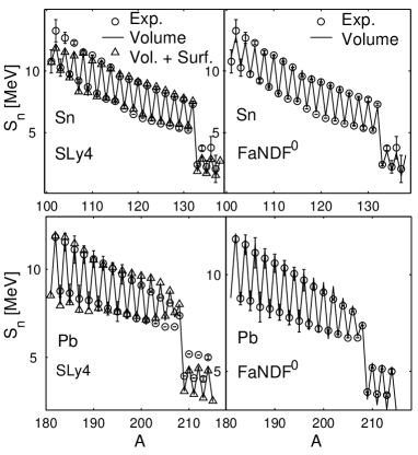
FIG. 1.: $S_{n}$ for tin and lead isotopes computed using the SLy4 EDF (left) and Fayans’ FaNDF⁰ (right) with either volume or half volume–half surface pairing.

We shall present here results only for those nuclei for which we can make comparison with available recommended nuclear masses [21]. We consider at first the tin (38 nuclei) and lead (34 nuclei) isotope chains. We performed a number of calculations of these isotopes essentially from the neutron to the proton drip lines, see Ref. [5] for some preliminary results. For these nuclei we can test only the sum of the coupling constants, namely $g(\mathchoice{{\hbox{\boldmath$\displaystyle r$}}}{{\hbox{\boldmath$\textstyle r$}}}{{\hbox{\boldmath$\scriptstyle r$}}}{{\hbox{\boldmath$\scriptscriptstyle r$}}})=g_{0}(\mathchoice{{\hbox{\boldmath$\displaystyle r$}}}{{\hbox{\boldmath$\textstyle r$}}}{{\hbox{\boldmath$\scriptstyle r$}}}{{\hbox{\boldmath$\scriptscriptstyle r$}}})+g_{1}(\mathchoice{{\hbox{\boldmath$\displaystyle r$}}}{{\hbox{\boldmath$\textstyle r$}}}{{\hbox{\boldmath$\scriptstyle r$}}}{{\hbox{\boldmath$\scriptscriptstyle r$}}})$. We have considered a bare coupling $g(\mathchoice{{\hbox{\boldmath$\displaystyle r$}}}{{\hbox{\boldmath$\textstyle r$}}}{{\hbox{\boldmath$\scriptstyle r$}}}{{\hbox{\boldmath$\scriptscriptstyle r$}}})=const$, which corresponds to volume pairing, and also $g(\mathchoice{{\hbox{\boldmath$\displaystyle r$}}}{{\hbox{\boldmath$\textstyle r$}}}{{\hbox{\boldmath$\scriptstyle r$}}}{{\hbox{\boldmath$\scriptscriptstyle r$}}})=V_{0}[1-\rho(\mathchoice{{\hbox{\boldmath$\displaystyle r$}}}{{\hbox{\boldmath$\textstyle r$}}}{{\hbox{\boldmath$\scriptstyle r$}}}{{\hbox{\boldmath$\scriptscriptstyle r$}}})/\rho_{c}]$, with parameters chosen to describe roughly one half volume and one half surface pairing, as suggested in particular in Ref. [7]. One–neutron separation energies $S_{n}$ and two–neutron separation energies $S_{2n}$ for tin and lead isotopes were computed for constant pairing $g(\mathchoice{{\hbox{\boldmath$\displaystyle r$}}}{{\hbox{\boldmath$\textstyle r$}}}{{\hbox{\boldmath$\scriptstyle r$}}}{{\hbox{\boldmath$\scriptscriptstyle r$}}})=const$, with mean–field computed with either SLy4 interaction [17] ($g(\mathchoice{{\hbox{\boldmath$\displaystyle r$}}}{{\hbox{\boldmath$\textstyle r$}}}{{\hbox{\boldmath$\scriptstyle r$}}}{{\hbox{\boldmath$\scriptscriptstyle r$}}})=-250\;{\mathrm{MeV}}\;{\mathrm{fm}}^{3}$) or with Fayans normal nuclear EDF [13] ($g(\mathchoice{{\hbox{\boldmath$\displaystyle r$}}}{{\hbox{\boldmath$\textstyle r$}}}{{\hbox{\boldmath$\scriptstyle r$}}}{{\hbox{\boldmath$\scriptscriptstyle r$}}})=-200{\mathrm{MeV}}\;{\mathrm{fm}}^{3}$). For the case of SLy4 interaction we also show results obtained for the half volume–half surface pairing model ($V_{0}=-370\;{\mathrm{MeV}}\;{\mathrm{fm}}^{3},\rho_{c}=0.32\;{\mathrm{fm}}^{-3}$). The search for the appropriate values for $g(\mathchoice{{\hbox{\boldmath$\displaystyle r$}}}{{\hbox{\boldmath$\textstyle r$}}}{{\hbox{\boldmath$\scriptstyle r$}}}{{\hbox{\boldmath$\scriptscriptstyle r$}}})$ was performed only among a finite set of values, e.g. in the case of volume pairing we considered $g=-200,-225,-250,-275$ and -300 ${\mathrm{MeV}}\;{\mathrm{fm}}^{3}$, see also Ref. [5].

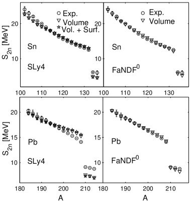
FIG. 2.: The same as in Fig. 1 but $S_{2n}$.

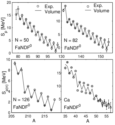
FIG. 3.: $S_{p}$ for isotone chains $N=$ 50, 82 and 126 and $S_{n}$ for calcium isotopes. For $S_{2p}$ and $S_{2n}$ see online report [22].

Table 1. Rms of $S_{2N}$ and $S_{N}$ deviations respectively from experiment [21] (in MeV’s) for several isotope and isotone chains.

Z or N	$S_{2N}/S_{N}$	$S_{2N}/S_{N}$	$S_{2N}$
chain	present	Ref. [11]	Ref. [23]
Z = 20	0.82/0.76	1.02/0.92	0.96
Z = 28	0.67/0.50	0.66/0.55	1.30
Z = 40	0.93/0.63	0.66/0.63	2.21
Z = 50	0.29/0.21	0.43/0.35	0.95
Z = 82	0.23/0.37	0.58/0.53	0.74
N = 50	0.37/0.26	0.41/0.23	NA
N = 82	0.43/0.31	0.50/0.56	NA
N = 126	0.42/0.23	0.88/0.52	NA

The agreement between experiment and theory is particularly good for the case of FaNDF⁰. We relate this result with the fact that the effective mass in FaNDF⁰ is the bare nucleon mass, unlike the case of SLy4 EDF and in agreement with the global mass fit of Ref. [11, 12]. It is notable that the agreement with experiment is equally good for both tin and lead isotopes with the same value of $g$, unlike Refs. [13]. Even though we used the same normal nuclear EDF as in Refs. [13], our agreement with experiment is notable superior, see Ref. [22], even though we parameterize the pairing interaction with one parameter only vs. up to five parameters used in these papers.

Since FaNDF⁰ in conjuction with the bare pairing coupling constant $g(\mathchoice{{\hbox{\boldmath$\displaystyle r$}}}{{\hbox{\boldmath$\textstyle r$}}}{{\hbox{\boldmath$\scriptstyle r$}}}{{\hbox{\boldmath$\scriptscriptstyle r$}}})=-200\;{\mathrm{MeV}}\;{\mathrm{fm}}^{3}$ apparently provides the best description in case of tin and lead isotopes, further calculations were performed only with this choice of parameters. In Fig. 3 we display the one–proton separation energies $S_{p}$ for three isotone chains (23 nuclei with $N=50$, 25 nuclei with $N=82$ and 14 nuclei with $N=126$) and $S_{n}$ for calcium isotopes (24 nuclei), and for nickel and zirconium isotopes see Ref. [22], 212 nuclei in total. Since the neutron numbers for these isotone chains are also magic, again, we can test only the same combination of coupling constants $g(\mathchoice{{\hbox{\boldmath$\displaystyle r$}}}{{\hbox{\boldmath$\textstyle r$}}}{{\hbox{\boldmath$\scriptstyle r$}}}{{\hbox{\boldmath$\scriptscriptstyle r$}}})=g_{0}(\mathchoice{{\hbox{\boldmath$\displaystyle r$}}}{{\hbox{\boldmath$\textstyle r$}}}{{\hbox{\boldmath$\scriptstyle r$}}}{{\hbox{\boldmath$\scriptscriptstyle r$}}})+g_{1}(\mathchoice{{\hbox{\boldmath$\displaystyle r$}}}{{\hbox{\boldmath$\textstyle r$}}}{{\hbox{\boldmath$\scriptstyle r$}}}{{\hbox{\boldmath$\scriptscriptstyle r$}}})$. As we have conjectured at the beginning of this study, one can indeed describe with a single value $g$ separately for proton and neutron pairing correlations in both even and odd systems, as opposed to the treatment of Refs. [11, 12], which slightly violates isospin invariance. In essentially all cases in which we have been able to perform a comparison between our results and those available in literature, our results were either qualitatively superior or, in a few separate cases, as good as any other results. In Table 1 we present rms deviation from experimental (recommended) values [21] for the two and one nucleon separation energies for several isotope and isotone chains. The size of each set of nuclei in a chain was given by the number of nuclei in Ref. [11], for which there are experimental values in the unpublished Audi and Wapstra 2001 compilation.

There are a number of theoretical arguments, suggesting that the pairing coupling should be density/position dependent, due to the coupling to surface/particle–hole modes, e.g. Ref. [24]. A similar line of reasoning was presented in the case of dilute systems [25, 26] and neutron matter [27, 28] for quite some time. Our results, see Figs. 1–2, show that $S_{n}$ and $S_{2n}$ for tin and lead isotopes are not particularly sensitive to such effects. To some extent this is not a surprise, since pairing correlations are ”built” at distances of the order of the coherence length $\xi\propto\hbar^{2}k_{F}/m\Delta$ [29], see Ref. [30] for a related instructive example. This apparent low sensitivity of $S_{N}$ and $S_{2N}$ to a possible density dependence of the pairing couplings, could in principle be profitably used to describe other observables. From the results of Refs. [26] one might infer that pairing coupling constants could have a noticeable variation with the isospin composition of a given system, since the magnitude of the induced interactions changes dramatically as the number of fermion species varies. Neither our results, nor previous work has necessitated the introduction of such a dependence however. In our phenomenological approach, based on general symmetry arguments alone and the fact that the pairing correlations are relatively weak in nuclear systems, we restricted the form of the EDF superfluid contribution to the simplest one compatible with known symmetries. We were able to infer that pairing properties of either kind of nucleons can be accounted for with a single constant $g=g_{0}+g_{1}$. It remains to be seen whether the other (non–perturbative) combination $g^{\prime}=g_{0}-g_{1}$ (never considered by other authors) could ever become relevant.

REFERENCES

- [1] P. Hohenberg and W. Kohn, Phys. Rev. 136, B864 (1964); W. Kohn and L.J. Sham, Phys. Rev. 140, A1133 (1965); R.M. Dreizler and E.K.U. Gross, Density Functional Theory: An Approach to the Quantum Many–Body Problem, (Springer, Berlin, 1990); R.G. Parr and W. Yang, Density–Functional Theory of Atoms and Molecules, Clarendon Press, Oxford (1989); W. Kohn, Rev. Mod. Phys. 71, 1253 (1999).
- [2] P. Ring, Prog. Part. Nucl. Phys. 37, 193 (1996); M. Bender et al., Phys. Lett. B 515, 42 (2002); P.–G. Reinhard et al., nucl-th/0012095; D.J. Dean and M. Hjorth–Jensen, Rev. Mod Phys. 75, 607 (2003); M. Bender et al., Rev. Mod. Phys. 75, 121 (2003); P. Ring and P. Schuck, The Nuclear Many–Body Problem, Springer, New York (1980).
- [3] A. Bulgac and Y. Yu, Phys. Rev. Lett. 88, 042504 (2002).
- [4] A. Bulgac, Phys. Rev. C 65, 051305(R) (2002).
- [5] A. Bulgac and Y. Yu, nucl-th/0109083.
- [6] J. Dobaczewski et al., Nucl. Phys. A 422, 103 (1984).
- [7] J. Dobaczewski et al., nucl-th/0109073; Eur.Phys. J. A15, 21 (2002).
- [8] H. Esbensen and G.F. Bertsch, Ann. Phys. 157 (1984) 255.
- [9] J. Dobaczewski et al., Phys. Rev. C 53, 2809 (1996); J. Dobaczewski et al., Nucl.Phys. A 693, 361 (2001); S. Sakakihara and Y. Tanaka, Nucl. Phys. A 691, 649 (2001); M. Bender et al., Eur. Phys. J. A 8, 59 (2000); T. Niksic et al., Phys.Rev. C66, 024306 (2002).
- [10] J. Dechargé and D. Gogny, Phys. Rev. C 21, 1568 (1980); J.F. Berger, et al., Comput. Phys. Comm. 63, 365 (1991).
- [11] S. Goriely et al., Phys. Rev. C 66, 024326 (2002).
- [12] D. Lunney et al., Rev. Mod. Phys. in press.
- [13] S.A. Fayans, JETP Letters, 68, 169 (1998); S.A. Fayans et al., Nucl. Phys. A 676, 49 (2000); S.A. Fayans et al., Phys. Lett. B 491, 245 (2000).
- [14] A. Bulgac and V.R. Shaginyan, Nucl. Phys. A 601, 103 (1996); ibid Phys. Lett. B 469, 1 (1999); B.A. Brown, Phys. Rev. C 58, 220 (1998); B.A. Brown,et al., Phys. Lett. B 483, 49 (2000).
- [15] A. Bulgac, preprint FT–194–1980, CIP, Bucharest; nucl-th/9907088.
- [16] S.T. Belyaev et al., Sov. J. Nucl. Phys. 45, 783 (1987).
- [17] E. Chabanat et al., Nucl. Phys. A 627, 710 (1997); Nucl. Phys. A 635, 231 (1998); Erratum Nucl. Phys. A 643, 441(E) (1998).
- [18] T. Papenbrock and G.F. Bertsch, Phys. Rev. C 59, 2052 (1999).
- [19] A.B. Migdal, Theory of Finite Fermi Systems and Applications to Atomic Nuclei, (Wiley Interscience, New York, 1967).
- [20] B. Friedman and V. R. Pandharipande, Nucl. Phys. A 361, 502 (1981); R. B. Wiringa, et al., Phys. Rev. C 38, 1010 (1988).
- [21] G. Audi and A. Wapstra Nucl. Phys. A 595, 409 (1995).
- [22] Y.Yu and A. Bulgac, nucl-th/0302007
- [23] S.Q. Zhang et al., nucl-th/0302032.
- [24] J. Terasaki et al., Nucl. Phys. A 697, 127 (2002).
- [25] L.P. Gorkov and T.K. Melik–Barkhudarov, Zh. Eksp. Teor. Fiz. 40, 1452 (1961) [Sov. Phys. JETP 13, 1018 (1961)].
- [26] H. Heiselberg et al. , Phys. Rev. Lett. 85, 2418 (2000); H.–J. Schulze et al., Phys. Rev. C 63, 044310 (2001).
- [27] J.M.C. Chen et al., Nucl. Phys. A 555, 59 (1993); J. Wambach et al., Nucl. Phys. A 555, 128 (1993).
- [28] U. Lombardo and H.–J. Schulze, Lect. Notes Phys. 578, 30 (2001) and astro-ph/0012209.
- [29] P.G. de Gennes, Superconductivity of Metals and Alloys, Addison–Wesley, Reading MA, (1998).; V.L. Ginzburg and L.D. Landau, Zh. Eksp. Teor. Fiz. 20, 1064 (1950).
- [30] Y. Yu and A. Bulgac, Phys. Rev. Lett. 90, 161101 (2003).