Abstract

Equation of State (EoS) for hot and dense nuclear matter with a quark-hadron phase transition is constructed within a statistical mixed-phase model assuming coexistence of unbound quarks in nuclear surrounding. This model predicts the deconfinement phase transition of the crossover type. The so-called ”softest point” effect of EoS is analyzed and confronted to that for other equations of state which exhibit the first order phase transition (two-phase bag model) or no transition at all (hadron resonance gas). The collective motion of nucleons from high-energy heavy-ion collisions is considered within a relativistic two-fluid hydrodynamics for different EoS. It is demonstrated that the beam energy dependence of the directed flow is a smooth function in the whole range from SIS till SPS energies and allows to disentangle different EoS, being in good agreement with experimental data for the statistical mixed-phase model. In contrast, excitation functions for relative strangeness abundance turn out to be insensitive to the order of phase transition.

Key-words: QCD phase transition, heavy-ion collisions, hydrodynamics, directed flow, strange particle production.

1 Introduction

The predicted phase transition from confined hadrons to a deconfined phase of their constituents (i.e. the asymptotically-free quarks and gluons or the so-called Quark-Gluon Plasma, QGP) is a challenge to the theory of strong interaction. Over the past two decades a lot of efforts has been spent to both the theoretical study of deconfinement phase transition and the search for its possible manifestation in relativistic heavy ion collisions, properties of neutron stars and Universe evolution. A unique opportunity provided by relativistic heavy-ion collisions allowed to reach a state with temperature and energy density exceeding the critical values, $T_{c}\sim 170\ MeV$ and $\varepsilon_{c}\sim 1\ GeV/fm^{3}$, specific for the deconfinement phase transition. A rather long list of various signals for the QGP formation in hot and dense nuclear matter is available now and it has been probed in experiments with heavy ions. Unfortunately, there is no crucial signal for unambiguous identification of the deconfinement phase and, for a particular reaction at the given bombarding energy, practically every proposed signal can be simulated to some extent by hadronic interactions.

In this paper we turn to the study of excitation functions for observables to be sensitive to the expected QCD deconfinement phase transition. Its manifestation has been considered already some time ago by [1, 2]. Since a phase transition slows down the time evolution of the system due to softening of the EoS, and one can expect a remarkable loss of correlations around some critical incident energy resulting in definite observable effects.

2 Equation of state in mixed phase model

Following the common strategy of the two-phase (2P) bag model [3], one can determine the deconfinement phase transition by means of the Gibbs conditions matching the EoS of a relativistic gas of hadrons and resonances, whose interactions are simulated by the Van der Waals excluded volume correction, to that of an ideal gas of quarks and gluons, where the change in vacuum energy in a QGP state is parameterized by the bag constant $B$. Thermodynamics of the hadron gas is described in the grand canonical ensemble. All hadrons with the mass $m_{j}<1.6\ GeV$ i are taken into consideration. One should emphasize that the phase transition in the 2P model is right along of the first order by constructing.

To reproduce the variety of phase transitions predicted by QCD lattice calculations we represent a phenomenological Mixed Phase (MP) model [4, 5]. The underlying assumption of the MP model is that unbound quarks and gluons may coexist with hadrons forming a homogeneous quark/gluon–hadron phase. Since the mean distance between hadrons and quarks/gluons in this mixed phase may be of the same order as that between hadrons, the interaction between all these constituents (unbound quarks/gluons and hadrons) plays an important role and defines the order of the phase transition.

Within the MP model [4, 5] the effective Hamiltonian is expressed in the quasiparticle approximation with density-dependent mean-field interactions. Under quite general requirements of confinement for color charges, the mean-field potential of quarks and gluons is approximated by

$$U_{q}(\rho)=U_{g}(\rho)={A\over\rho^{\gamma}}~{};\ \ \ \gamma>0$$ (1)

with the total density of quarks and gluons

$$\rho=\rho_{q}+\rho_{g}+\sum\limits_{j}\;\nu_{j}\rho_{j}~{},$$

where $\rho_{q}$ and $\rho_{g}$ are the densities of unbound quarks and gluons outside of hadrons, while $\rho_{j}$ is the density of hadron type $j$ and $\nu_{j}$ is the number of valence quarks inside. The presence of the total density $\rho$ in (1) implies interactions between all components of the mixed phase. The approximation (1) mirrors two important limits of the QCD interaction. For $\rho\to 0$, the interaction potential approaches infinity, i.e. an infinite energy is necessary to create an isolated quark or gluon, which simulates the confinement of color objects. In the other extreme case of large energy density corresponding to $\rho\to\infty$, we have $U_{q}=U_{g}=0$ which is consistent with asymptotic freedom.

The use of the density-dependent potential (1) for quarks and the hadronic potential, described by a modified non-linear mean-field model [6], requires certain constraints to be fulfilled, which are related to thermodynamic consistency [4, 5]. For the chosen form of the Hamiltonian these conditions require that $U_{g}(\rho)$ and $U_{q}(\rho)$ do not depend on temperature. From these conditions one also obtains a form for the quark–hadron potential [4].

A detailed study of the pure gluonic $SU(3)$ case with a first-order phase transition allows one to fix the values of the parameters as $\gamma=0.92$ and $\displaystyle A^{1/(3\gamma+1)}=250$ MeV. These values are then used for the $SU(3)$ system including quarks. As is shown in Fig.1 for the case of quarks of two light flavors at zero baryon density ($n_{B}=0$), the MP model is consistent with lattice QCD data providing a continuous phase transition if the crossover type with a deconfinement temperature $T_{dec}=153$ MeV. For a two-phase approach based on the bag model a first-order deconfinement phase transition occurs with a sharp jump in energy density $\varepsilon$ at $T_{dec}$ close to the value obtained from lattice QCD.

Figure 1: The reduced energy density and pressure (the $\varepsilon_{SB}$ and $p_{SB}$ are corresponding Stephan-Boltzmann quantities) of the $SU(3)$ system with two light flavors for $n_{B}=0$ calculated within the MP (solid lines) and bag (dashed lines) models. Circles and squares are lattice QCD data obtained within the Wilson [7] and Kogut–Susskind [8] schemes.

Though at a glimpse the temperature dependencies of the energy density $\varepsilon$ and pressure $p$ for the different approaches presented in Fig.1 look quite similar, there is a large difference revealed when $p/\varepsilon$ is plotted versus $\varepsilon$ (cf. Fig.2, left panel). The lattice QCD data differ at low $\varepsilon$, which is due to difficulties within the Kogut–Susskind scheme [8] in treating the hadronic sector. A particular feature in the MP model is that, for $n_{B}=0$, the softest point of the EoS, defined as a minimum of the function $p(\varepsilon)/\varepsilon$ [9], is not

Figure 2: The ($\varepsilon,p/\varepsilon$)-representation of the EoS for the two-flavor $SU(3)$ system at various baryon densities $n_{B}$. Notation of data points and lines is the same as in Fig.1.

very pronounced and located at comparatively low values of the energy density: $\varepsilon_{SP}\approx 0.45$ GeV/fm³, which roughly agrees with the lattice QCD value [7]. This value of $\varepsilon$ is close to the energy density inside a nucleon, and hence, reaching this value indicates that we are dealing with a single big hadron consisting of deconfined matter. In contradistinction, the bag-model EoS exhibits a very pronounced softest point at large energy density $\varepsilon_{SP}\approx 1.5$ GeV/fm³ [9, 10].

The MP model can be extended to baryon-rich systems in a parameter-free way [4, 5]. As demonstrated in Fig.2 (right panel), the softest point for baryonic matter is gradually washed out with increasing baryon density and vanishes for $n_{B}\mathrel{\hbox to0.0pt{ \lower 4.0pt\hbox{\hskip-3.0pt$\sim$}\hss}\raise 1.0pt\hbox{$>$}}0.3\ n_{0}$ ($n_{0}$ is normal nuclear matter density). This behavior differs drastically from that of the two-phase bag-model EoS, where $\varepsilon_{SP}$ is only weakly dependent on $n_{B}$ [9, 10]. It is of interest to note that the interacting hadron gas model has no softest point at all and, in this respect, its thermodynamic behavior is close to that of the MP model at high energy densities [5].

These differences between the various models of EoS should manifest themselves in dynamics discussed below.

3 Directed flow of baryons

The EoS described above is applied to a two-fluid (2F) hydrodynamic model [11], which takes into account finite stopping power of colliding heavy ions. In this dynamical model, the total baryonic current and energy-momentum tensor are written as

$$J^{\mu} = J^{\mu}_{p}+J^{\mu}_{t}~{}~{},$$ (2)

$$T^{\mu\nu} = T^{\mu\nu}_{p}+T^{\mu\nu}_{t}~{}~{},$$ (3)

where the baryonic current $J^{\mu}_{\alpha}=n_{\alpha}u_{\alpha}^{\mu}$ and energy-momentum tensor $T^{\mu\nu}_{\alpha}$ of the fluid $\alpha$ are initially associated with either target ($\alpha=t$) or projectile ($\alpha=p$) nucleons. Later on these fluids contain all hadronic and quark–gluon species, depending on the model used for describing the fluids. The twelve independent quantities (the baryon densities $n_{\alpha}$, 4-velocities $u_{\alpha}^{\mu}\;$ normalized as $u_{\alpha\mu}u_{\alpha}^{\mu}=1$, as well as temperatures $T$ and pressures $p$ of the fluids) are obtained by solving the following set of equations of two-fluid hydrodynamics [11]

$$\partial_{\mu}J_{\alpha}^{\mu} = 0~{}~{},$$ (4)

$$\partial_{\mu}T^{\mu\nu}_{\alpha} = F_{\alpha}^{\nu}~{}~{},$$ (5)

where the coupling term

$$F_{\alpha}^{\nu}=n^{s}_{p}n^{s}_{t}\left<V_{rel}\int d\sigma_{NN\to NX}(s)\;(p-p_{\alpha})^{\nu}\right>$$ (6)

characterizes friction between the counter-streaming fluids. The cross sections $d\sigma_{NN\to NX}$ take into account all elastic and inelastic interactions between the constituents of different fluids at the invariant collision energy $s^{1/2}$ with the local relative velocity $V_{rel}=[s(s-4m_{N}^{7})]^{1/2}/2m_{N}^{2}~{}.$ The average in (6) is taken over all particles in the two fluids which are assumed to be in local equilibrium intrinsically [11]. The set of Eqs. (4) and (5) is closed by EoS, which is naturally the same for both colliding fluids.

Following the original paper [11], it is assumed that a fluid element decouples from the hydrodynamic regime, when its baryon density $n_{B}$ and densities in the eight surrounding cells become smaller than a fixed value $n_{f}$. A value $n_{f}=0.8n_{0}$ is used for this local freeze-out density which corresponds to the actual density of the freeze-out fluid element of about $0.6-0.7\ n_{0}$.

The directed flow characterizes the deflection of emitted hadrons away from the beam axis within the reaction $x-z$ plane. In particular, one defines the differential directed flow by the mean in-plane component $\left<p_{x}(y)\right>$ of the transverse momentum at a given rapidity $y$. This deflection is believed to be quite sensitive to the elasticity or softness of the EoS and can be quantified in two ways: In terms of the derivative (a slope parameter) at mid-rapidity

$$F_{y}=\left.\frac{d\;\left<p_{x}(y)\right>}{dy}\right|_{y=y_{cm}}~{}~{},$$ (7)

which is quite suitable for analyzing the flow excitation function, and by another integral quantity to be less sensitive to possible rapidity fluctuations of the in-plane momentum:

$$\left<P_{x}\right>=\frac{\displaystyle\int dp_{x}dp_{y}dy\ p_{x}\ \left(E{\displaystyle\frac{d^{3}N}{dp^{3}}}\right)}{\displaystyle\int dp_{x}dp_{y}dy\ \left(E{\displaystyle\frac{d^{3}N}{dp^{3}}}\right)}~{}~{},$$ (8)

where the integration in the c.m.system runs over the rapidity region $\displaystyle[0,y_{cm}]$. Excitation functions in the SIS-AGS-SPS energy range are plotted in Fig.3 for both characteristics [12].

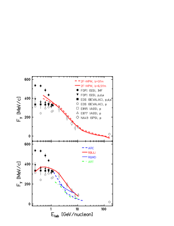
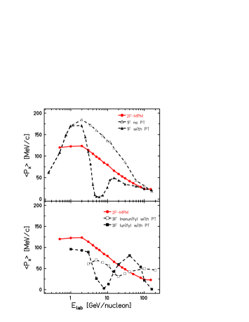
Figure 3: Excitation functions of the slope parameter $F_{y}$ (left panel) and the average directed flow (right panel) for baryons from Au + Au collisions within hydrodynamics and different transport simulations. Collected experimental points are taken from [12]. The results of transport calculations for three different codes (left lower panel) are given by the thin solid (RQMD), dashed (ARC) and dot-dashed (ART) lines (cited according to [13]). The solid line (RBUU) is taken from [14]. 2F hydrodynamics with the MP EoS at the impact parameter 3 fm is compared with the corresponding results of 1F- [10] (right upper panel) and 3F- (right lower panel) [15] hydrodynamics with the bag-model EoS. 1F calculations both with and without the phase transition (PT) are displayed.

Our first 2F hydrodynamic calculations of $F_{y}(E_{lab})$ are in a good agreement with experiment in the whole energy range considered. In the left lower panel of Fig.3 our results are compared with transport calculations. The ARC and ART are cascade models, while the RQMD takes also into account mean-field effects. Though all these models agree with experimental data at $E_{lab}\approx 10$ A$\cdot$GeV (considered as a reference point), values of $F_{y}$ at lower energies are clearly underestimated, as is evident from comparison with results of the E895 Collaboration [16] (see empty squares in Fig.3). Recently, a good description of experimental points (including the E895 data) was reported within a relativistic BUU (RBUU) model [14]. The good agreement with experiment was achieved here by a special fine tuning of the mean fields involved in the particle propagation.

The calculated excitation functions of $\left<P_{x}\right>$ for baryons within different hydrodynamic models are shown in the right panel of Fig.3. Conventional 1F hydrodynamics for pure hadronic matter [10] results in a very large directed flow due to the inherent instantaneous stopping of the colliding matter. This instantaneous stopping is unrealistic at high beam energies. If the deconfinement phase transition, based on the bag-model EoS [10], is included into this model, the excitation function of $\left<P_{x}\right>$ exhibits a deep minimum near $E_{lab}\approx 6$ A$\cdot$GeV, which manifests the softest-point effect of the bag-model EoS as shown in the right panel of Fig.2.

The result of 2F hydrodynamics with the MP EoS noticeably differs from the 1F calculations. After a maximum around 1 A$\cdot$GeV, the average directed flow decreased slowly and smoothly. This difference is caused by two reasons. First, as follows from Fig.2, the softest point of the MP EoS is washed out for $n_{B}\mathrel{\hbox to0.0pt{ \lower 4.0pt\hbox{\hskip-3.0pt$\sim$}\hss}\raise 1.0pt\hbox{$>$}}0.4$. The second reason is dynamical: the finite stopping power and direct pion emission change the evolution pattern. The latter point is confirmed by comparison to three-fluid calculations with the bag EoS [15] plotted in the right lower panel of Fig.3. The third pionic fluid in this model is assumed to interact only with itself neglecting the interaction with baryonic fluids. Therefore, with regard to the baryonic component, this three-fluid hydrodynamics [15, 17] is completely equivalent to our two-fluid model and the main difference is due to the different EoS. As seen in Fig.3, the minimum of the directed flow excitation function, predicted by the one-fluid hydrodynamics with the bag-model EoS, survives in the three-fluid (nonunified) regime but its value decreases and its position shifts to higher energies. If one applies the unification procedure of  [15], which favors fusion of two fluids into a single one, and thus making stopping larger, three-fluid hydrodynamics practically reproduces the one-fluid result and predicts in addition a bump at $E_{lab}\approx 40$ A$\cdot$GeV.

4 Strangeness production

Enhanced strangeness production as compared to proton-proton or proton-nucleus collisions is one of the QGP signals proposed a long time ago. In the hydrodynamic model described above only baryon charge rather than strangeness exchange is included. So, to see experimental consequences of EoS with different phase transition order, we consider an expanding homogeneous blob of the compressed and heated QCD matter (a fireball) formed in heavy-ion collisions. The initial state ($\varepsilon_{0}$ and $n_{B}$) for this fireball is estimated from results of the QGSM transport calculations in the center-of-mass frame inside a cylinder of the volume $V_{0}$ with radius $R=5\ fm$ and Lorentz-contracted length $L=2R/\gamma_{c.m.}$. Isoentropic expansion is treated in an approximate manner assuming $V\sim V_{0}t$ until the freeze-out point defined by $\varepsilon_{f}=0.15\ GeV/fm^{3}\approx m_{N}n_{0}$ (for more detail see [18]).

One should note that till this point the grand canonical ensemble was used where complete chemical equilibrium is assumed and the strangeness conservation is controlled on average by the strange chemical potential $\mu_{S}$. In the thermodynamical limit, fluctuations in a number of strange particles are small and coincide with those for the canonical ensemble. However, it is not the case for finite systems at relatively small $T$ where the strangeness canonical ensemble should be applied, taking into account the associative nature of strange particle creation by exact and local conservation of strangeness. Using the general formalism for the canonical strangeness conservation proposed in [19, 20], the partition function of a gas of hadrons with strangeness $s_{i}=0,\pm 1,\pm 2,\pm 3$ and total strangeness $S=0$ can be written as follows

$$Z_{S}=\frac{1}{2\pi}\int_{-\pi}^{\pi}d\phi\ \exp(\sum_{s=-3}^{3}{\cal S}_{s}\ e^{is\phi})$$ (9)

where ${\cal S}_{s}=V\sum_{i}Z_{i}~{}.$ Here $Z_{i}$ is the one-particle partition function for species $i$ and the sum is taken over all particles and resonances carrying strangeness $s_{i}$. A number of strange particles can be found by the appropriate differentiation of the partition function $Z_{S}$, Eq.(9). It is easy to see that canonical result can be obtain in the Boltzmann approximation from the grand canonical one by replacing the strange fugacity in the following way :

$$\exp(\mu_{s}/T)\to\left(\frac{{\cal S}_{1}}{\sqrt{{\cal S}_{1}{\cal S}_{-1}}}\right)^{s}\ \frac{I_{s}(x)}{I_{0}(x)}~{},$$ (10)

where the argument of the Bessel functions $x\equiv 2\sqrt{{\cal S}_{1}{\cal S}_{-1}}\sim V$. This receipt was applied to our treatment of particle abundance at the freeze-out point. Generally, the correlation volume in the suppression factor $I_{s}(x)/I_{0}(x)$ of (10) does not coincide with the system volume $V$. In our model, the initial Lorentz-contracted volume $V_{0}$ is considered as a strangeness correlation volume.

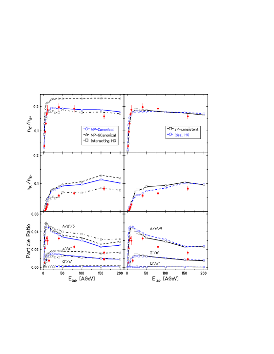
Figure 4: Particle ratios for strange hadrons in full $4\pi$ angle interval for central $Au+Au$ collision as a function of bombarding energy. The compilation of available experimental points is taken from [21, 22]. The calculated excitation functions represent four modeling EoS with the canonical suppression factor $I_{s}(x)/I_{0}(x)$. For the case of the MP model, the grand canonical results (dashed lines) are given, as well.

Inspection of Fig.4 shows that the inclusion of the canonical strangeness suppression factor allows one to decrease noticeably strange particle abundance. However, comparing canonical and grand canonical results for the MP model, one can see that they do not coincide at high energies as it would be expected. This is explained by the beam energy dependence of the strangeness correlation volume in contrast with usual canonical description [19, 20]. The most striking result followed from Fig.4 is that all the models considered in the strangeness canonical ensemble predict practically the same relative abundance of strange hadrons in the whole energy range studied. The measured excitation function for $K^{+}/\pi^{+}$ are reproduced reasonably well excluding maybe the SIS energy. In the case of $K^{-}/\pi^{-}$ the general form of excitation functions also agrees with experimental one but the relative abundance is overestimated what mainly originates from neglecting the electric charge (isospin) conservation. A simple estimate shows that taking into account the isospin conservation the $K^{-}/\pi^{-}$ ratio decreases by about $18\%$ and $12\%$ at $E_{lab}=10$ and $150\ AGeV$, respectively, without any essential influence on the $K^{+}/\pi^{+}$ ratio. The relative yield of hyperons, in particular $\Lambda/\pi^{+}$’s, seems to be overshot in the energy range $E_{lab}\mathrel{\hbox to0.0pt{ \lower 4.0pt\hbox{\hskip-3.0pt$\sim$}\hss}\raise 1.0pt\hbox{$<$}}\ 10\ AGeV$ what can result from the simplified dynamical treatment: The Bjorken-like longitudinal expansion can be applied at the SPS energies, but at the SIS energies the transverse expansion is not negligible. It is worthy to note that all calculations have been done with the same shock-like freeze-out condition for every EoS without any special tuning.

5 Conclusions

It has been shown that the directed flow excitation functions $F_{y}$ and $\left<P_{x}\right>$ for baryons are sensitive to the EoS, but this sensitivity is significantly masked by nonequilibrium dynamics of nuclear collisions. Nevertheless, the results indicate that the widely used two-phase EoS, based on the bag model [9, 10] and giving rise to a first-order phase transition, seems to be inappropriate. The neglect of interactions near the deconfinement temperature results in an unrealistically strong softest-point effect within this two-phase EoS. Smooth experimental excitation function of the directed flow is reasonably reproduced within the MP model.

The dynamical trajectories for a fireball state in the $T-\mu_{B}$ plane are quite different for different EoS [18, 23]. However, after using the shock-like freeze-out, the global strangeness production is turned out to be completely insensitive to the particular EoS as illustrated by the calculation of excitation functions for $K^{+},K^{-}$ and hyperons. To get agreement with experiment the canonical suppression factor should be taken into account. The only trace of dynamics is the beam-energy dependence of the strangeness correlation volume. This effect results in a negative slope of the $K^{+}/\pi^{+}$ excitation function at high energies which is not reproduced by the equilibrium statistical model with canonical account of strangeness [20, 21].

Among other signals of the QCD deconfinement phase transition, the dilepton and hard photon production is the most promising. Being sensitive to the whole evolution time of a system, these signals can become experimentally observable to disentangle the crossover phase transition, predicted by the MP model, from the first order one which is peculiar for the bag-model EoS.

Useful and numerous discussions with B. Friman, Yu.B. Ivanov, E.G. Nikonov, W. Nörenberg and K. Redlich are acknowledged. This work was supported in part by DFG (project 436 RUS 113/558/0) and RFBR (grant 00-02-04012).

References

- [1] E. Shuryak and O.V. Zhirov, Phys. Lett. B 89, 253 (1979).
- [2] L. van Hove, Z. Phys. C 21, 93 (1983).
- [3] J. Cleymans, R.V. Gavai, and E. Suhonen, Phys. Rep. 130, 217 (1986).
- [4] E.G. Nikonov, A.A. Shanenko, and V.D. Toneev, Heavy Ion Physics 8 (1998) 89.
- [5] V.D. Toneev, E.G. Nikonov, and A.A. Shanenko, in Nuclear Matter in Different Phases and Transitions, eds. J.-P. Blaizot, X. Campi, and M. Ploszajczak, Kluwer Academic Publishers (1999), p.309.
- [6] J. Zimanyi et al., Nucl. Phys. A484, 147 (1988).
- [7] K. Redlich and H. Satz, Phys. Rev. D 33, 3747 (1986).
- [8] C. Bernard et al., Nucl. Phys. (Proc. Suppl.) B47, 499 (1996); ibid 503.
- [9] C.M. Hung and E.V. Shuryak, Phys. Rev. Lett. 75, 4063 (1995).
-
[10]
D.H. Rischke et al.,
Heavy Ion Physics 9, 309 (1996);
D.H. Rischke, Nucl. Phys. A610, 28c (1996). -
[11]
I.N. Mishustin, V.N. Russkikh, and
L.M. Satarov, Nucl. Phys. A494, 595 (1989);
Yad. Fiz. 54, 479 (1991) (translated as Sov. J. Nucl. Phys. 54, 260 (1991). - [12] Yu.B. Ivanov, E.G. Nikonov, W. Nörenberg, A.A. Shanenko and V.D. Toneev, Heavy Ion Physics 15 (2002) 117.
- [13] N.N. Ajitanand et al., Nucl. Phys. A638, 451c (1998).
- [14] P.K. Sahu, W. Cassing, U. Mosel, and A. Ohnishi, Nucl. Phys. A672, 376 (2000).
- [15] J. Brachmann et al., Phys. Rev. C 61, 024909 (2000).
- [16] H. Liu for the E895 Collaboration, Nucl. Phys. A638, 451c (1998).
- [17] J. Brachmann et al., Nucl. Phys. A619, 391 (1997).
- [18] B. Friman, E.G. Nikonov, W. Nörenberg, K. Redlich and V.D. Toneev, Strangeness Production in Nuclear Matter and Expansion Dynamics (in preparation).
- [19] R. Hagedorn and K. Redlich, Z. Phys. A 27, 541 (1985).
- [20] J. Cleymans, K. Redlich, and E. Suhonen, Z. Phys. C 51, 137 (1991).
- [21] K. Redlich, Nucl. Phys. A698, 94 (2002).
- [22] The NA49 Collaboration, nucl-ex/0205002.
- [23] V.D. Toneev, J. Cleymans, E.G. Nikonov, K. Redlich, and A.A. Shanenko, J. Phys. G 27, 827 (2001).