Pairing in nuclear systems: from neutron stars to finite nuclei

Abstract

We discuss several pairing-related phenomena in nuclear systems, ranging from superfluidity in neutron stars to the gradual breaking of pairs in finite nuclei. We focus on the links between many-body pairing as it evolves from the underlying nucleon-nucleon interaction and the eventual experimental and theoretical manifestations of superfluidity in infinite nuclear matter and of pairing in finite nuclei. We analyse the nature of pair correlations in nuclei and their potential impact on nuclear structure experiments. We also describe recent experimental evidence that points to a relation between pairing and phase transitions (or transformations) in finite nuclear systems. Finally, we discuss recent investigations of ground-state properties of random two-body interactions where pairing plays little role although the interactions yield interesting nuclear properties such as 0⁺ ground states in even-even nuclei.

I INTRODUCTION

Pairing lies at the heart of nuclear physics and the quantum many-body problem in general. In this review we address some of the recent theoretical and experimental studies of pairing phenomena in finite nuclei and nuclear matter. In infinitely extended nuclear systems, such as neutron star matter and nuclear matter, the study of superfluidity and pairing has a long history, see e.g., Migdal (1960); Cooper et al. (1959); Emery and Sessler (1960), even predating the 1967 discovery of pulsars Hewish et al. (1968), which were soon identified as rapidly rotating magnetic neutron stars Gold (1969). Interest in nucleonic pairing has intensified in recent years, owing primarily to experimental developments on two different fronts. In the field of astrophysics, a series of $X$-ray satellites (including Einstein, EXOSAT, ROSAT, and ASCA) has brought a flow of data on thermal emission from neutron stars, comprising both upper limits and actual flux measurements. The recent launching of the Chandra $X$-ray observatory provides further impetus for more incisive theoretical investigations. On the terrestrial front, the expanding capabilities of radioactive-beam and heavy-ion facilities have stimulated a concerted exploration of nuclei far from stability, with a special focus on neutron-rich species Riisager (1994); Mueller and Sherril (1993). Pairing plays a prominent role in modeling the structure and behavior of these newly discovered nuclei.

Since the field is quite vast, we limit our discussion to several recent advances that have taken place. We will focus in particular on two overlapping questions: (i) how does many-body pairing evolve from the bare nucleon-nucleon interaction, and (ii) what are the experimental (and perhaps theoretical) manifestations of pairing in finite nuclei? Over fifty years ago, Mayer Mayer (1950) pointed out that a short-ranged, attractive, nucleon-nucleon interaction would yield $J=0$ ground states. The realistic bare nucleon-nucleon potential indeed contains short-range attractive parts (particularly in the singlet-$S$ and triplet-$P$ channels) that give rise to pairing in infinite nuclear matter and nuclei. In this Review, we will discuss various calculations that demonstrate this effect. We will also demonstrate the link between superfluidity in nuclear matter and its origin from realistic nucleon-nucleon interactions. We then study the nature of pair correlations in nuclei, their potential impact on nuclear structure experiments, and the origin of pairing in the presence of a random two-body interaction. We conclude with recent experimental evidence that points to a relation between pairing and phase transitions (or transformations) in finite nuclear systems.

Before we present the outline of this work, we feel that some historical remarks about the particularity of the pairing problem in nuclear physics may be appropriate.

I.1 Theory of pairing in nuclear physics

In 1911 Kamerlingh Onnes discovered superconductivity in condensed matter systems, and its microscopic explanation came about through the highly successful pairing theory proposed in 1957 by Bardeen, Cooper, and Schrieffer (BCS) Cooper et al. (1957). A series of first applications to nuclear structure followed Bohr et al. (1958); Belyaev (1959); Migdal (1959). The BCS theory also generalized the seniority coupling scheme in which pair-wise coupling of equivalent nucleons to a state of zero angular momentum takes place. The scheme had been developed during years previous to the discovery of BCS theory Racah (1942); Mayer (1950); Racah and Talmi (1953).

BCS applications in nuclear structure calculations incorporate two inherent drawbacks. First, the BCS wave function is not an eigenstate of the number operator, so that number fluctuation is an issue. Second, there is a critical value of the pairing-force strength for which no non-trivial solution exists. Several attempts were made to overcome these problems: calculating the random phase approximation (RPA) in addition to BCS Unna and Weneser (1965); including particle number projection Kerman et al. (1961) after variation, valid for pairing strengths above the critical pairing strength, and a projection before variation that works well for all pairing strength values. A simplified prescription for the latter is a technique known as the Lipkin-Nogami method Lipkin (1960); Nogami (1964). It has been quite successful in overcoming some of the shortfalls that occur when BCS is applied to nuclei; see e.g., the recent works of Hagino et al. Hagino and Bertsch (2000); Hagino et al. (2002) and references therein. Of course, BCS is an approximate solution to the many-body problem and assumes a particular form for the many-body wave function. Another, more drastic, approximation to the many-body problem assumes that a single Slater determinant suffices to describe the nuclear ground state. This mean-field solution to the many-body problem gives rise to Hartree-Fock (HF) theory. An effective nucleon-nucleon potential describes the nuclear interaction, and is typically a parameterization of the Skyrme zero-range force Skyrme (1956, 1959); Vautherin and Brink (1970, 1972). Solutions of the HF equations describe various nuclear ground-state properties sufficiently Quentin and Flocard (1978), but they do not include an explicit pairing interaction. Finite-range interactions, such as the Gogny interaction Decharge et al. (1975), when used in Hartree-Fock calculations has also no pairing by construction. A general way to include pairing into a mean-field description generated by e.g., a Skyrme interaction requires solving the Hartree-Fock-Bogoliubov (HFB) equations Bogolyubov (1959). Recent applications to both stable and weakly bound nuclei may be found in, e.g., Dobaczewski et al. (1996); Duguet et al. (2002a, b). A renormalization scheme for the HFB equations was recently proposed by Bulgac and Yu for a zero range pairing interaction Bulgac (2002); Bulgac and Yu (2002). Rather than solving the full HFB equations, one may first calculate the Hartree-Fock single-particle wave functions and use these as a basis for solving the BCS equations Tondeur (1979); Nayak and Pearson (1995). For stable nuclei with large one- or two-neutron separation energies, the HF+BCS approximation to HFB is valid, but the technique is not able to adequately address weakly bound nuclei due to the development of a particle (usually neutron) gas on or near the nuclear surface.

While nuclear mean-field calculations represent a well-founded method to describe nuclear properties, their results do not represent complete solutions to the nuclear many-body problem. Short of a complete solution to the many-nucleon problem Pudliner et al. (1995), the interacting shell model is widely regarded as the most broadly capable description of low-energy nuclear structure and the one most directly traceable to the fundamental many-body problem. While this is a widely accepted statement, applications of the shell model to finite nuclei encounter several difficulties. Chief among these is the choice of the interaction. A second problem involves truncations of the Hilbert space, and a third problem involves the numerics of solving extremely large eigenvalue problems.

Skyrme and Gogny forces are parameterized nuclear forces, but they lack a clear link to the bare nucleon-nucleon interaction as described by measured scattering phase shifts. The same philosophy has been used for shell-model interactions, e.g., with the USD $1s$-$0d$-shell interaction Wildenthal (1984b). While quite successful, these types of interactions cannot be related directly to the nucleon-nucleon interaction either. The shell model then becomes a true model with many parameters. Alternatively, many attempts have been made to derive an effective nucleon-nucleon interaction in a given shell-model space from the bare nucleon-nucleon interaction using many-body perturbation theory. (For a modern exposition on this difficult problem, see Hjorth-Jensen et al. (1995) and references therein.) While this approach appears to work quite well for many nuclei, there are several indications Pudliner et al. (1995, 1997); Pieper et al. (2001) that an effective interaction based on a two-body force only fails to reproduce experimental data. As shown in e.g., Pudliner et al. (1995, 1997); Pieper et al. (2001), these difficulties are essentially related to the absence of a real three-body interaction. It should be noted, however, that the deficiencies of the effective interactions are minimal and affect the ground-state energies more than they affect the nuclear spectroscopy. Thus, understanding various aspects of physics from realistic two-body interactions, or their slightly modified, yet more phenomenological, cousins, is still a reasonable goal.

I.2 Outline

This work starts with an overview of pairing in infinite matter, with an emphasis on superfluidity and superconductivity in neutron stars. As an initial theme, we focus on the link between superfluidity in nuclear matter and its origin from realistic nucleon-nucleon interactions. This is done in Sec. II where we discuss pairing in neutron star matter and symmetric nuclear matter. Thereafter, we focus on various aspects of pairing in finite nuclei, from spectroscopic information in Sec. III to pairing from random interactions in Sec. IV and thermodynamical properties in Sec. V. Concluding remarks are presented in Sec. VI. The paragraphs below serve as an introduction to the exposed physics.

I.2.1 Pairing in neutron stars

The presence of neutron superfluidity in the crust and the inner part of neutron stars are considered well established in the physics of these compact stellar objects. To a first approximation, a neutron star is described as a neutral system of nucleons (and possibly heavier baryons) and electrons (and possibly muons) in beta equilibrium at zero temperature, with a central density several times the saturation density $\rho_{0}$ of symmetrical nuclear matter Heiselberg and Hjorth-Jensen (2000); Pethick (1992); Shapiro and Teukolsky (1983); Lamb (1991); Wiringa et al. (1988); Alpar et al. (1995). The gross structure of the star (mass, radius, pressure, and density profiles) is determined by solving the Tolman-Oppenheimer-Volkov general relativistic equation of hydrostatic equilibrium, consistently with the continuity equation and the equation of state (which embodies the microscopic physics of the system). The star contains (i) an outer crust made up of bare nuclei arranged in a lattice interpenetrated by relativistic electrons, (ii) an inner crust where a similar Coulomb lattice of neutron-rich nuclei is embedded in Fermi seas of relativistic electrons and neutrons, (iii) a quantum fluid interior of coexisting neutron, proton, and electron fluids, and finally (iv) a core region of uncertain constitution and phase (but possibly containing hyperons, a pion or kaon condensate, and/or quark matter). Fig. 1 gives a schematic portrait of a possible neutron star structure.

In the low-density outer part of a neutron star, the neutron superfluidity is expected mainly in the attractive singlet ${}^{1}S_{0}$ channel. Qualitatively, this phenomenon can be understood as follows. At the relatively large average particle spacing at the “low” densities involved in this region, i.e., $\rho\sim\rho_{0}/10$ with $\rho_{0}$ the saturation density of symmetrical nuclear matter, the neutrons experience mainly the attractive component of the ${}^{1}S_{0}$ interaction; however, the pairing effect is quenched at higher densities, $\sim\rho_{0}$ and beyond, due to the strong repulsive short-range component of this interaction. At higher density, the nuclei in the crust dissolve, and one expects a region consisting of a quantum liquid of neutrons and protons in beta equilibrium. By similar reasoning, one thus expects ${}^{1}S_{0}$ proton pairing to occur in the quantum fluid interior, in a density regime where the proton contaminant (necessary for charge balance and chemical equilibrium) reaches a partial density $\rho_{p}\sim\rho_{0}/10$. In this region, neutron superfluidity is expected to occur mainly in the coupled ${}^{3}P_{2}$-${}^{3}F_{2}$ two-neutron channel. At such densities, one may also expect superfluidity from other baryons such as, e.g., hyperons to arise. The possibility for hyperon pairing is an entirely open issue; see, for example, Balberg and Barnea (1997). Neutron, proton, and eventual hyperon superfluidity in the ${}^{1}S_{0}$ channel, and neutron superfluidity in the ${}^{3}P_{2}$ channel, have been shown to occur with gaps of a few MeV or less Baldo et al. (1998b); however, the density ranges in which gaps occur remain uncertain. In the core of the star any superfluid phase should finally disappear, although the possibility of a color superconducting phase may have interesting consequences. At large baryon densities for which perturbative QCD applies, pairing gaps for like quarks have been estimated to be a few MeV D. and Love (1984). However, the pairing gaps of unlike quarks ($ud,~{}us$, and $ds$) have been suggested to be several tens to hundreds of MeV through non-perturbative studies Alford et al. (1999) kindling interest in quark superfluidity and superconductivity Son (1999) and their effects on neutron stars.

A realistic ab initio prediction of the microscopic physics of nucleonic superfluid components in the interiors of neutron stars is crucial to a quantitative understanding of neutrino cooling mechanisms Friman and Maxwell (1979); Tsuruta (1979); Takatsuka and Tamagaki (1997); Tsuruta (1998) that operate immediately after their birth in supernova events, as well as the magnetic properties, vortex structure, rotational dynamics, and pulse timing irregularities of these superdense stellar objects. In particular, when nucleonic species enter a superfluid state in one or another region of the star, suppression factors of the form $\exp(-\Delta_{F}/k_{B}T)$ are introduced into the expression for the emissivity, $\Delta_{F}$ being an appropriate average measure of the energy gap at the Fermi surface. Pairing thus has a major effect on the star’s thermal evolution through suppressions of neutrino emission processes and specific heats as well; see, for example, Page et al. (2000).

I.2.2 Pairing phenomena in nuclei

After the excursion to infinite matter, we return to the question concerning how to obtain information on pairing correlations in finite nuclei from abundantly available spectroscopic data. We discuss this point in Sec. III. Even in the presence of random interactions, signatures of pairing still remain in finite many-body systems. In Sec. IV we present a discussion of pairing derived from random interactions.

Apart from relatively weak electric forces, the interactions between two protons are very similar to those between two neutrons. This yields the idea of charge symmetry of the nuclear forces. Furthermore, the proton-neutron interaction is also very similar. This led very early to the idea of isotopic invariance of the nucleon-nucleon interaction. A nucleon with quantum number isospin $\tau=1/2$ may be in one of two states, $\tau_{z}=-1/2$ (proton) or $\tau_{z}=+1/2$ (neutron). Of course, the symmetry is not exact, but is widely employed when discussing nuclei. It leads to a quantum number $T$ called isospin, and its projection $T_{z}=(N-Z)/2$, where the number of neutrons (protons) in the nucleus is $N$ ($Z$).

We can define with this isospin symmetry two distinct states within the two-nucleon system. A $T=1$ nucleon-nucleon system can have spin-projection $T_{z}=1,0,-1$. $T_{z}=1$ corresponds to a neutron-neutron system, $T_{z}=0$ to a proton-neutron system, and $T_{z}=-1$ to a proton-proton system. The nucleons in this case have total spin $J=0$ in order for the full wave function to maintain antisymmetry of the total nucleon-nucleon wave function. For the same reason, $T=0$ proton-neutron systems can only have $T_{z}=0$ and $J=1$. Thus, two different types of elementary particle pairs exist in the nucleus, and they depend on both the spin and isospin quantum numbers of the two-particle system.

This brief discussion of the general quantum numbers of a two-nucleon system is a natural starting point for a discussion of pairing found in nuclei. All even-even nuclei have a ground-state with total angular momentum quantum number and parity, $\pi$, $J^{\pi}=0^{+}$. One can postulate a pairing interaction that couples particles in time-reversed states. Using this type of simple pairing interaction, one can also understand the fact that in even-even nuclei the ground state is rather well separated from excited states, although in the even-odd neighbor nucleus, several states exist near the ground state.

The behavior of the even-even ground state is usually associated with isovector ($T=1$) pairing of the elementary two-body system. Simplified models of the nucleon-nucleon interaction, such as the seniority model Talmi (1993), predict a pair condensate in these systems. An open question concerns evidence for isoscalar ($T=0$) pairing in nuclei. One unique aspect of nuclei with $N$=$Z$ is that neutrons and protons occupy the same shell-model orbitals. Consequently, the large spatial overlaps between neutron and proton single-particle wave functions are expected to enhance neutron-proton ($np$) correlations, especially the $np$ pairing.

At present, it is not clear what the specific experimental fingerprints of the $np$ pairing are, whether the $np$ correlations are strong enough to form a static condensate, and what their main building blocks are. Most of our knowledge about nuclear pairing comes from nuclei with a sizable neutron excess where the isospin $T$=1 neutron-neutron ($nn$) and proton-proton ($pp$) pairing dominate. Now, for the first time, there is an experimental opportunity to explore nuclear systems in the vicinity of the $N$=$Z$ line which have many valence $np$ pairs; that is, to probe the interplay between the like-particle and neutron-proton ($T$=0,1, $T_{z}$=0) pairing channels. One evidence related to $T=0$ pairing involves the Wigner energy, the extra binding that occurs in $N=Z$ nuclei. We will discuss this in more detail in Sec. III.

One possible way to experimentally access pair correlations in nuclei is by neutron-pair transfer, see e.g., Yoshida (1962). Simply stated, if the ground-state of a nucleus is made of BCS pairs of neutrons, then two-neutron transfer should be enhanced when compared to one-neutron transfer. Collective enhancement of pair transfer is expected if nuclei with open shells are brought into contact Peter et al. (1999). Pairing fluctuations are also expected in rapidly rotating nuclei Shimizu et al. (1989). In lighter systems, such as ⁶He, two-neutron transfer has been used for studying the wave function of the ground state Oganessian et al. (1999).

Finally, we discuss phenomenological descriptions of nuclear collective motion where the nuclear ground state and its low-lying excitations are represented in terms of bosons. In one such model, the Interacting Boson Model (IBM), $L=0$ (S) and $L=2$ (D) bosons are identified with nucleon pairs having the same quantum numbers Iachello and Arima (1988), and the ground state can be viewed as a condensate of such pairs. Shell-model studies of the pair structure of the ground state and its variation with the number of valence nucleons can therefore shed light on the validity and microscopic foundations of these boson approaches.

I.2.3 Thermodynamic properties of nuclei and level densities

The theory of pairing in nuclear physics is also strongly related to other fields of physics, such as distinct gaps in ultrasmall metallic grains in the solid state. These systems share in common the fact that the energy spectrum of a system of particles confined to a small region is quantized. It is only recently, through a series of experiments by Tinkham et al. Ralph et al. (1995); Black et al. (1996, 1997), that spectroscopic data on discrete energy levels from ultrasmall metallic grains (with sizes of the order of a few nanometers and mean level spacings less than millielectron-volts) has been obtained by way of single-electron-tunneling spectroscopy. Measurements in solid state have been much more elusive due to the size of the system. The discrete spectrum could not be resolved due to the energy scale set by temperature. Of interest here is the observation of so-called parity effects. Tinkham et al. Ralph et al. (1995); Black et al. (1996, 1997) were able to observe the number parity (odd or even) of a given grain by studying the evolution of the discrete spectrum in an applied magnetic field. These effects were also observed in experiments on large Al grains. It was noted that an even grain had a distinct spectroscopic gap whereas an odd grain did not. This is clear evidence of superconducting pairing correlations in these grains. The spectroscopic gap was driven to zero by an applied magnetic field; hence the paramagnetic breakdown of pairing correlations could be studied in detail. For theoretical interpretations, see, for example, von Delft and Ralph (2001); Balian et al. (1999); Mastellone and Falci (1998); Dukelsky and Sierra (1999).

In the smallest grains with sizes less than 3 nanometers, such distinct spectroscopic gaps could however not be observed. This vanishing gap revived an old issue: what is the lower size of a system for the existence of superconductivity is such small grains?

A nucleus is also a small quantal system, with discrete spectra and strong pairing correlations. However, whereas the statistical physics of the above experiments on ultrasmall grains can be well described through a canonical ensemble, i.e., a system in contact with a heat bath, the nucleus in the laboratory is an isolated system with no heat exchange with the environment. The appropriate ensemble for its description is the microcanonical one Balian et al. (1999). This poses significant interpretation problems. For example, is it possible to define a phase transition in an isolated quantal system such as a nucleus?

In Sec. V we attempt to link our discussion to such topics via recent experimental evidence of pairing from studies of level densities in rare-earth nuclei. The nuclear level density, the density of eigenstates of a nucleus at a given excitation energy, is the important quantity that may be used to describe thermodynamic properties of nuclei, such as the nuclear entropy, specific heat, and temperature. Bethe first described the level density using a non-interacting fermi gas model for the nucleons Bethe (1936). Modifications to this picture, such as the back-shifted fermi gas which includes pair and shell effects Gilbert and Cameron (1965); Newton (1956) not present in Bethe’s original formulation, are in wide use. These modifications incorporate long-range pair correlations that play an important role in the low excitation region. Experimentalists recently developed methods Henden et al. (1995); Tveter et al. (1996) to extract level densities at low spin from measured $\gamma$-spectra.

There is evidence for the existence of paired nucleons (Cooper pairs) at low temperature. In high-spin nuclear physics, the backbending phenomenon is a beautiful manifestation of the breaking of pairs. The mechanism induced by Coriolis forces tends to align single particle angular momenta along the nuclear rotational axis Stephens and Simon (1972); Johnson et al. (1971); Riedinger et al. (1980); Faessler et al. (1976). Theoretical models also predict a reduction in the pair correlations at higher temperatures Mottelson and Valantin (1960); Muhlhans et al. (1983); Døssing et al. (1995). There is also an interesting connection between quasiparticle spectra in metallic grains and high-spin spectra in nuclei. In nuclei it is the Coriolis force that acts on pairs of nucleons and plays thus a role similar to the magnetic field acting on Cooper pairs of electrons.

The breaking of pairs is difficult to observe as a function of intrinsic excitation energy. Recent theoretical Døssing et al. (1995) and experimental Tveter et al. (1996); Melby et al. (1999) works indicate that the process of breaking pairs takes place over several MeV of excitation energy. Thus, the phenomenon of pair breaking in a finite-fermi system behaves somewhat differently than what would be expected in nuclear matter. The corresponding critical temperature in finite systems is measured to be $T_{c}\sim$ 0.5 MeV/$k_{B}$ Schiller et al. (2001), where $k_{B}$ is Boltzmann’s constant. Recent work extracted the entropy of the ^161,162Dy and ^171,172Yb isotopes and deduced the number of excited quasiparticles as a function of excitation energy. We describe this result in more detail in Sec. V.

II PAIRING IN INFINITE MATTER AND THE NUCLEON-NUCLEON INTERACTION

Pairing correlations and the phenomenon of superconductivity and superfluidity are intimately related to the underlying interaction whether it is, for example, the nucleon-nucleon (NN) interaction or the interaction between ³He atoms. In this section we discuss, through simple examples, some of the connections between pairing correlations as they arise in nuclear systems and the bare NN interaction itself, that is, the interaction of a pair of nucleons in free space. The latter is most conveniently expressed in terms of partial waves (and their pertaining quantum numbers such as orbital angular momentum and total spin) and phase shifts resulting from nucleon-nucleon scattering experiments. Actually, without specializing to some given fermionic systems and interactions, it is possible to relate the pairing gap and the BCS theory of pairing to the experimental phase shifts. This means, in turn, that we can, through an inspection of experimental scattering data, understand which partial waves may yield a positive pairing gap and eventually lead to, e.g., a superfluid phase transition in an infinite fermionic system. We show this in subsec. II.3 (although we limit the attention to nuclear interactions), after we have singled out those partial waves and interaction properties which are expected to be crucial for pairing correlations in both nuclei and neutron stars. These selected features of the NN interaction are discussed in the next subsection. A brief overview of superfluidity in neutron stars and pairing in symmetric nuclear matter is presented in subsec. II.4, with an emphasis on those partial waves of the NN interaction which are expected to produce a finite pairing gap. Features of neutron-proton pairing in infinite matter are reviewed in subsec. II.4.2. Concluding remarks, open problems, and perspectives are presented in the last subsection.

II.1 Selected features of the nucleon-nucleon interaction

The interaction between nucleons is characterized by the existence of a strongly repulsive core at short distances, with a characteristic radius $\sim 0.5-1$ fm. The interaction obeys several fundamental symmetries such as translational, rotational, spatial-reflection, time-reversal invariance and exchange symmetry. It also has a strong dependence on quantum numbers such as total spin $S$ and isospin $T$, and, through the nuclear tensor force which arises from, e.g., one-pion exchange, it also depends on the angles between the nucleon spins and separation vector. The tensor force thus mixes different angular momenta $L$ of the two-body system, that is, it couples two-body states with total angular momentum $J=L-1$ and $J=L+1$. For example, for a proton-neutron two-body state, the tensor force couples the states ${}^{3}S_{1}$ and ${}^{3}D_{1}$, where we have used the standard spectroscopic notation ${}^{2S+1}L_{J}$.

Although there is no unique prescription for how to construct an NN interaction, a description of the interaction in terms of various meson exchanges is presently the most quantitative representation, see for example Machleidt (1989); Wiringa et al. (1995); Stoks et al. (1994); Machleidt et al. (1996); Machleidt (2001), in the energy regime of nuclear structure physics. We will assume that meson-exchange is an appropriate picture at low and intermediate energies. Further, in our discussion of pairing, it suffices at the present stage to limit our attention to the time-honored configuration-space version of the nucleon-nucleon (NN) interaction, including only central, spin-spin, tensor and spin-orbit terms. In our notation below, the mass of the nucleon $M_{N}$ is given by the average of the proton and neutron masses. The interaction reads (omitting isospin)

$$V({\bf r})=\left\{C^{0}_{C}+C^{1}_{C}+C_{\sigma}\mbox{\boldmath$\sigma$}_{1}\cdot\mbox{\boldmath$\sigma$}_{2}+C_{T}\left(1+{3\over m_{\alpha}r}+{3\over\left(m_{\alpha}r\right)^{2}}\right)S_{12}(\hat{r})+C_{SL}\left({1\over m_{\alpha}r}+{1\over\left(m_{\alpha}r\right)^{2}}\right){\bf L}\cdot{\bf S}\right\}\frac{e^{-m_{\alpha}r}}{m_{\alpha}r},$$ (1)

where $m_{\alpha}$ is the mass of the relevant meson and $S_{12}$ is the tensor term

$$S_{12}(\hat{r})=\mbox{\boldmath$\sigma$}_{1}\cdot\mbox{\boldmath$\sigma$}_{2}\mbox{\boldmath$\hat{r}$}^{2}-\mbox{\boldmath$\sigma$}_{1}\cdot\mbox{\boldmath$\hat{r}$}\cdot\mbox{\boldmath$\sigma$}_{2}\cdot\mbox{\boldmath$\hat{r}$},$$ (2)

where $\sigma$ is the standard operator for spin $1/2$ particles. Within meson-exchange models, we may have, e.g., the exchange of $\pi,\eta,\rho,\omega,\sigma$, and $\delta$ mesons. As an example, the coefficients for the exchange of a $\pi$ meson are $C_{\sigma}=C_{T}={g_{NN\pi}^{2}\over 4\pi}\frac{m^{3}_{\pi}}{12M_{N}^{2}}$, and $C^{0}_{C}=C^{1}_{C}=C_{SL}=0$ with the experimental value for $g_{NN\pi}^{2}\approx 13-14$; see, for example, Machleidt (2001) for a recent discussion.

The pairing gap is determined by the attractive part of the NN interaction. In the ${}^{1}S_{0}$ channel the potential is attractive for momenta $k\leq 1.74$ fm^-1 (or for interparticle distances $r\geq 0.6$ fm), as can be seen from Fig. 2. In the weak coupling regime, where the interaction is weak and attractive, a gas of fermions may undergo a superconducting (or superfluid) instability at low temperatures, and a gas of Cooper pairs is formed. This gas of Cooper pairs will be surrounded by unpaired fermions and the typical coherence length is large compared with the interparticle spacing, and the bound pairs overlap. With weak coupling we mean a regime where the coherence length is larger than the interparticle spacing. In the strong-coupling limit, the formed bound pairs have only a small overlap, the coherence length is small, and the bound pairs can be treated as a gas of point bosons. One expects then the system to undergo a Bose-Einstein condensation into a single quantum state with total momentum $k=0$ Nozieres and Schmitt-Rink (1985). For the ${}^{1}S_{0}$ channel in nuclear physics, we may actually expect to have two weak-coupling limits, namely when the potential is weak and attractive for large interparticle spacings and when the potential becomes repulsive at $r\approx 0.6$ fm. In these regimes, the potential has values of typically some few MeV. One may also loosely speak of a strong-coupling limit where the NN potential is large and attractive. This takes place where the NN potential reaches its maximum, with an absolute value of typically $\sim 100$ MeV, at roughly $\sim 1$ fm, see again Fig. 2. We note that fermion pairs in the ${}^{1}S_{0}$ wave in neutron and nuclear matter will not undergo the above-mentioned Bose-Einstein condensation, since, even though the NN potential is large and attractive for certain Fermi momenta, the coherence length will always be larger than the interparticle spacing, as demonstrated by De Blasio et al. De Blasio et al. (1997). The inclusion of in-medium effects, such as screening terms, are expected to further reduce the pairing gap and thereby enhance further the coherence length. This does not imply that such a transition is not possible in nuclear matter. A recent analysis by Lombardo et al. Lombardo and Schuck (2001); Lombardo et al. (2001a) of triplet ${}^{3}S_{1}$ pairing in low-density symmetric and asymmetric nuclear matter indicates that such a transition is indeed possible.

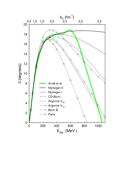
Figure 4: ${}^{3}P_{2}$ phase-shift predictions of different potentials up to $E_{\rm lab}=1.1\;{\rm GeV}$, compared with the phase shift analysis of Arndt et al. Arndt et al. (1997).

Hitherto we have limited our attention to one single partial wave, the ${}^{1}S_{0}$ channel. Our discussion about the relation among the NN interaction, its pertinent phase shifts, and the pairing gap, can be extended to higher partial waves as well. An inspection of the experimental phase shifts for waves with $J\leq 2$ and total isospin $T=1$, see Fig. 3, reveals that there are several partial waves which exhibit attractive (positive phase shifts) contributions to the NN interaction. Such attractive terms are in turn expected to yield a possible positive pairing gap. This means that the energy dependence of the nucleon-nucleon ($NN$) phase shifts in different partial waves offers some guidance in judging what nucleonic pair-condensed states are possible or likely in different regions of a neutron star. A rough correspondence between baryon density and $NN$ bombardment energies can be established through the Fermi momenta assigned to the nucleonic components of neutron-star matter. The lab energy relates to the Fermi energy through $E_{\mathrm{lab}}=4\epsilon_{F}=4\hbar^{2}k_{F}^{2}/2M_{N}$. This is demonstrated in Fig. 4 for various NN interaction models that fit scattering data up to $E_{\mathrm{lab}}\approx 350$ MeV. For comparison, we include results for older potential models such as the Paris Lacombe et al. (1980), $V_{14}$ Wiringa et al. (1984) and Bonn B Machleidt (1989) interactions. Note, as well, that beyond the point where these potential models have been fit, there is a considerable variation. This has important consequences for reliable predictions of the ${}^{3}P_{2}$ pairing gap.

In pure neutron matter, only $T=1$ partial waves are allowed. Moreover, one need only consider partial waves with $L\leq 4$ in the range of baryon density – optimistically, $\rho<(3-4)\rho_{0}$ – where a nucleonic model of neutron-star material is tenable, where $\rho_{0}=0.16$ fm^-3 is the saturation density of nuclear matter. We have already seen that the ${}^{1}S_{0}$ phase shift is positive at low energy (indicating an attractive in-medium force) but turns negative (repulsive) at around 250 MeV lab energy. Thus, unless the in-medium pairing force is dramatically different from its vacuum counterpart, the situation already suggested above should prevail: S-wave pairs should form at low densities but should be inhibited from forming when the density approaches that of ordinary nuclear matter.

The next lowest $T=1$ partial waves are the three triplet P waves ${}^{3}P_{J}$, with $J=0,1,2$. For the the ${}^{3}P_{0}$ state, the phase shift is positive at low energy, turning negative at a lab energy of 200 MeV. The attraction is, however, not sufficient to produce a finite pairing gap in neutron star matter. The ${}^{3}P_{1}$ phase shift is negative at all energies, indicating a repulsive interaction. The ${}^{3}P_{2}$ phase shift is positive for energies up to 1 GeV and is the most attractive $T=1$ phase shift at energies above about 160 MeV. Whereas the ${}^{1}S_{0}$ partial wave is dominated by the central force contribution of the NN interaction, see Eq. (1), the main contribution to the attraction seen in the ${}^{3}P_{2}$ partial wave stems from the two-body spin-orbit force for intermediate ranges in Eq. (1), i.e., the term proportional with ${\bf L}\cdot{\bf S}$. This is demonstrated in Fig. 5 where we plot the coordinate space version of the Argonne $V_{18}$ interaction Wiringa et al. (1995) with and without the spin-orbit contribution. Moreover, there is an additional enhancement due to the ${}^{3}P_{2}$–${}^{3}F_{2}$ tensor force. A substantial pairing effect in the ${}^{3}P_{2}$–${}^{3}F_{2}$ channel may hence be expected at densities somewhat in excess of $\rho_{0}$, again assuming that the relevant in-vacuum interaction is not greatly altered within the medium.

The remaining $T=1$ partial waves with $L\leq 4$ are both singlets: ${}^{1}D_{2}$ and ${}^{1}G_{4}$. However, the phase shifts of these partial waves, albeit being positive over the energy domain of interest, do not provide any substantial contribution to the pairing gap. Thus, only the ${}^{1}S_{0}$ and ${}^{3}P_{2}$ partial waves yield enough attraction to produce a finite pairing gap in pure neutron matter. Singlet and triplet pairing are hence synonomous with ${}^{1}S_{0}$ and ${}^{3}P_{2}$–${}^{3}F_{2}$ pairing, respectively.

II.2 Pairing gap equations

The gap equation for pairing in non-isotropic partial waves is, in general, more complex than in the simplest singlet $S$-wave case, in particular in neutron and nuclear matter, where the tensor interaction can couple two different partial waves Tamagaki (1970); Takatsuka and Tamagaki (1993); Baldo et al. (1995). This is indeed the situation for the ${}^{3}P_{2}$-${}^{3}F_{2}$ neutron channel or the ${}^{3}S_{1}$-${}^{3}D_{1}$ channel for symmetric nuclear matter. For the sake of simplicity, we disregard for the moment spin degrees of freedom and the tensor interaction. Starting with the Gorkov equations Schrieffer (1964), which involve the propagator $G(\bm{k},\omega)$, the anomalous propagator $F(\bm{k},\omega)$, and the gap function $\Delta(\bm{k})$, we have

$$\left(\begin{array}[]{rr}\omega-\epsilon(\bm{k})&-\Delta(\bm{k})\\ -\Delta^{\dagger}(\bm{k})&\omega+\epsilon(\bm{k})\end{array}\right)\left(\begin{array}[]{c}G\\ F^{\dagger}\end{array}\right)(\bm{k},\omega)=\left(\begin{array}[]{c}1\\ 0\end{array}\right)\>,$$ (9)

where $\epsilon(\bm{k})=e(\bm{k})-\mu$, $\mu$ being the chemical potential and $e(\bm{k})$ the single-particle spectrum. The quasi-particle energy $E(\bm{k})$ is the solution of the corresponding secular equation and is given by

$$E(\bm{k})^{2}=\epsilon(\bm{k})^{2}+|\Delta(\bm{k})|^{2}\>.$$ (10)

The anisotropic gap function $\Delta(\bm{k})$ is to be determined from the gap equation

$$\Delta(\bm{k})=-\sum_{\bm{k}^{\prime}}\langle\bm{k}|V|\bm{k}^{\prime}\rangle{\Delta(\bm{k}^{\prime})\over 2E(\bm{k}^{\prime})}\>.$$ (11)

The angle-dependent energy denominator in this equation prevents a straightforward separation into the different partial wave components by expanding the potential,

$$\langle\bm{k}|V|\bm{k}^{\prime}\rangle=4\pi\sum_{L}(2L+1)P_{L}(\bm{\hat{k}\cdot\hat{k}^{\prime}})V_{L}(k,k^{\prime})\>,$$ (12)

and the gap function,

$$\Delta(\bm{k})=\sum_{L,M}\sqrt{4\pi\over 2l+1}Y_{LM}(\bm{\hat{k}})\Delta_{LM}(k),$$ (13)

with $L$ and $M$ being the total orbital momentum and its projection, respectively. The functions $Y_{L,M}$ are the spherical harmonics. However, after performing an angle average approximation for the gap in the quasi-particle energy,

$$|\Delta(\bm{k})|^{2}\rightarrow D(k)^{2}\equiv{1\over 4\pi}\int d\bm{\hat{k}}\,|\Delta(\bm{k})|^{2}=\sum_{L,M}{1\over 2L+1}|\Delta_{LM}(k)|^{2}\>,$$ (14)

the kernels of the coupled integral equations become isotropic, and one can see that the different $m$-components become uncoupled and all equal. One obtains the following equations for the partial wave components of the gap function:

$$\Delta_{L}(k)=-{1\over\pi}\int_{0}^{\infty}k^{\prime}dk^{\prime}{V_{L}(k,k^{\prime})\over\sqrt{\epsilon(k^{\prime})^{2}+\left[\sum_{L^{\prime}}\Delta_{L^{\prime}}(k^{\prime})^{2}\right]}}\Delta_{L}(k^{\prime})\>.$$ (15)

Note that there is no dependence on the quantum number $M$ in these equations; however, they still couple the components of the gap function with different orbital momenta $L$ (${}^{1}S_{0}$, ${}^{3}P_{0}$, ${}^{3}P_{1}$, ${}^{3}P_{2}$, ${}^{1}D_{2}$, ${}^{3}F_{2}$, etc. in neutron matter) via the energy denominator. Fortunately, in practice the different components $V_{L}$ of the potential act mainly in non-overlapping intervals in density, and therefore also this coupling can usually be disregarded.

The addition of spin degrees of freedom and of the tensor force does not change the picture qualitatively and is explained in detail in Takatsuka and Tamagaki (1993); Baldo et al. (1995). The only modification is the introduction of an additional $2\times 2$ matrix structure due to the tensor coupling of the ${}^{3}P_{2}$ and ${}^{3}F_{2}$ channels. Such coupled channel equations can be written as

$$\left(\begin{array}[]{c}\Delta_{L}\\ \Delta_{L^{\prime}}\end{array}\right)(k) = -{1\over\pi}\int_{0}^{\infty}dk^{\prime}k^{\prime 2}{1\over E(k^{\prime})}\left(\begin{array}[]{rr}V_{LL}&-V_{LL^{\prime}}\\ -V_{L^{\prime}L}&V_{L^{\prime}L^{\prime}}\end{array}\right)(k,k^{\prime})\left(\begin{array}[]{c}\Delta_{L}\\ \Delta_{L^{\prime}}\end{array}\right)(k^{\prime})\>,$$ (22)

$$E(k)^{2} = [\epsilon(k)-\epsilon(k_{F})]^{2}+D(k)^{2}\>,$$ (23)

$$D(k)^{2} = \Delta_{L}(k)^{2}+\Delta_{L^{\prime}}(k)^{2}\>.$$ (24)

Here $\epsilon(k)=k^{2}/2m+U(k)$ are the single-particle energies of a neutron with momentum $k$, and $k_{F}$ is the Fermi momentum. The orbital momenta $L$ and $L^{\prime}$ could, e.g., represent the ${}^{3}P_{2}$ and ${}^{3}F_{2}$ channel, respectively. Restricting the attention to only one partial wave, it is easy to get the equation for an uncoupled channel like the ${}^{1}S_{0}$ wave, i.e., we obtain

$$\Delta(k)_{L}=-\frac{1}{\pi}\int_{0}^{\infty}dk^{\prime}k^{\prime 2}V_{LL}(k,k^{\prime}){{\Delta(k^{\prime})}\over{E(k^{\prime})}},$$ (25)

where $V_{LL}(k,k^{\prime})$ is now the bare momentum-space NN interaction in the ${}^{1}S_{0}$ channel, and $E(k)$ is the quasiparticle energy given by $E(k)=\sqrt{(\epsilon(k)-\epsilon(k_{F}))^{2}+\Delta(k)_{L}^{2}}$.

The quantities

$$V_{LL^{\prime}}(k,k^{\prime})=\int_{0}^{\infty}drr^{2}j_{L^{\prime}}(k^{\prime}r)V_{LL^{\prime}}(r)j_{L}(kr)$$ (26)

are the matrix elements of the bare interaction in the different coupled channels, e.g., $(T=1;\;S=1;\,J=2;\,L,L^{\prime}=1,3)$. It has been shown that the angle average approximation is an excellent approximation to the true solution that involves a gap function with ten components Takatsuka and Tamagaki (1993); Kodel et al. (1996), as long as one is only interested in the average value of the gap at the Fermi surface, $\Delta_{F}\equiv D(k_{F})$, and not the angular dependence of the gap functions $\Delta_{L}(\bm{k})$ and $\Delta_{L^{\prime}}(\bm{k})$.

Recently Khodel, Khodel, and Clark Kodel et al. (2001, 1998) proposed a separation method for the triplet pairing gap, based on Kodel et al. (1996), which allows a generalized solution of the BCS equation that is numerically reliable, without employing an angle-average approach. We refer the reader to Kodel et al. (1996, 2001, 1998) for more details. In this approach, the pairing matrix elements are written as a separable part plus a remainder that vanishes when either momentum variable is on the Fermi surface. This decomposition effects a separation of the problem of determining the dependence of the gap components in a spin-angle representation on the magnitude of the momentum (described by a set of functions independent of magnetic quantum number) from the problem of determining the dependence of the gap on angle or magnetic projection. The former problem is solved through a set of nonsingular, quasilinear equations Kodel et al. (2001, 1998). There is, in general, a good agreement between their approach and the angle average scheme. However, the general scheme of Khodel, Khodel, and Clark offers a much more stable algorithm for solving the pairing gap equations for any channel and starting with the bare interaction itself. In nuclear physics the interaction typically has a strongly repulsive core, a fact that can complicate significantly the iterative solution of the BCS equations.

An important ingredient in the calculation of the pairing gap is the single-particle potential $U(k)$. The gap equation is extremely sensitive to both many-body renormalizations of the interaction and the similar corrections to the single-particle energies. Many-body renormalizations of the interaction will be discussed in Sec. II.5. In our discussion below, we will present results for various many-body approaches to $U(k)$, from $U(k)=0$ to results with different Brueckner-Hartree-Fock (BHF) calculations, with both a discontinuous choice, a model-space BHF approach and within the “continuous-choice” scheme Jeukenne et al. (1976).

The single-particle energies appearing in the quasiparticle energies (10) and (24) are typically obtained through a self-consistent BHF calculation, using a $G$-matrix defined through the Bethe-Brueckner-Goldstone equation as

$$G=V+V\frac{Q}{\omega-H_{0}}G,$$ (27)

where $V$ is the nucleon-nucleon potential, $Q$ is the Pauli operator which prevents scattering into intermediate states prohibited by the Pauli principle, $H_{0}$ is the unperturbed Hamiltonian acting on the intermediate states, and $\omega$ is the starting energy, the unperturbed energy of the interacting particles. Methods to solve this equation are reviewed in Hjorth-Jensen et al. (1995). The single-particle energy for state $k_{i}$ ($i$ encompasses all relevant quantum numbers like momentum, isospin projection, spin, etc.) in nuclear matter is assumed to have the simple quadratic form

$$\epsilon_{k_{i}}={\displaystyle\frac{k_{i}^{2}\hbar^{2}}{2M^{*}_{N}}}+\delta_{i},$$ (28)

where $M_{N}^{*}$ is the effective mass. The terms $M_{N}^{*}$ and $\delta$, the latter being an effective single-particle potential related to the $G$-matrix, are obtained through the self-consistent BHF procedure. The model-space BHF (MBHF) method for the single-particle spectrum has also been used, see, for example, Hjorth-Jensen et al. (1995), with a cutoff momentum $k_{M}=3.0$ fm${}^{-1}>k_{F}$. In this approach the single-particle spectrum is defined by

$$\epsilon_{k_{i}}=\frac{k_{i}^{2}\hbar^{2}}{2M_{N}}+u_{i},$$ (29)

with the single-particle potential $u_{i}$ given by

$$u_{i}=\left\{\begin{array}[]{cc}\sum_{k_{h}\leq k_{F}}\left\langle k_{i}k_{h}|G(\omega=\epsilon_{k_{i}}+\epsilon_{k_{h}})|k_{i}k_{h}\right\rangle_{AS},&k_{i}\leq k_{M},\\ 0,k_{i}>k_{M},\end{array}\right.,$$ (30)

where the subscript $AS$ denotes antisymmetrized matrix elements. This prescription reduces the discontinuity in the single-particle spectrum as compared with the standard BHF choice $k_{M}=k_{F}$. The self-consistency scheme consists of choosing adequate initial values of the effective mass and $\delta$. The obtained $G$-matrix is then used to calculate the single-particle potential $u_{i}$, from which we obtain new values for $m^{*}$ and $\delta$. This procedure continues until these parameters vary little.

Recently, Lombardo et al. Lombardo et al. (2001b); Lombardo and Schulze (2001) have reanalyzed the importance of the various approaches to the single-particle energies. Especially, they demonstrate that the energy dependence of the self-energy can deeply affect the magnitude of the energy gap in a strongly correlated Fermi system; see also the recent works of Bozek in Bozek (1999, 2000, 2002). We will discuss these effects in Subsec. II.5.

II.3 Simple relations between the interaction and the pairing gap for identical particles

II.3.1 The low density limit

A general two-body Hamiltonian can be written in the form $\hat{H}=\hat{H}_{1}+\hat{H}_{2}$ where

$$\hat{H}_{1} = \sum_{\alpha}\varepsilon_{\alpha}a^{\dagger}_{\alpha}a_{\alpha}\;,$$ (31)

$$\hat{H}_{2} = \sum_{\alpha\beta\gamma\delta}V_{\alpha\beta\gamma\delta}a^{\dagger}_{\alpha}a^{\dagger}_{\beta}a_{\delta}a_{\gamma}\;,$$ (32)

where $a^{\dagger}$ and $a$ are fermion creation and annihilation operators, and $V$ are the uncoupled matrix elements of the two-body interaction. The sums run over all possible single-particle quantum numbers.

We limit the discussion in this section to a Fermi gas model with two-fold degeneracy and a pairing-type interaction as an example; i.e., the degeneracy of the single-particle levels is set to $2s+1=2$, with $s=1/2$ being the spin of the particle. We specialize to a singlet two-body interaction with quantum numbers $l=0$ and $S=0$, that is a ${}^{1}S_{0}$ state, with $l$ the relative orbital momentum and $S$ the total spin. For this partial wave, the NN interaction is dominated by the central component in Eq. (1), which, within a meson-exchange picture, can be portrayed through $2\pi$ (leading to an effective $\sigma$ meson) and higher $\pi$ correlations in order to yield enough attraction at intermediate distances.

At low densities, the interaction can be characterized by its scattering length only in order to get expansions for the energy density or the excitation spectrum. For the nucleon-nucleon interaction, the scattering length is $a_{0}=-18.8\pm 0.3$ fm for neutron-neutron scattering in the ${}^{1}S_{0}$ channel. If we first assume discrete single-particle energies, the scattering length approximation leads to the following approximation of the two-body Hamiltonian of Eq. (32)

$$H=\sum_{i}\varepsilon_{i}a^{\dagger}_{i}a_{i}+\frac{1}{2}G\sum_{ij>0}a^{\dagger}_{i}a^{\dagger}_{\bar{\imath}}a_{\bar{\jmath}}a_{j}.$$ (33)

The indices $i$ and $j$ run over the number of levels $L$, and the label $\bar{\imath}$ stands for a time-reversed state. The parameter $G$ is now the strength of the pairing force, while $\varepsilon_{i}$ is the single-particle energy of level $i$. Introducing the pair-creation operator $S^{+}_{i}=a^{\dagger}_{im}a^{\dagger}_{i-m}$, one can rewrite the Hamiltonian in Eq. (33) as

$$H=d\sum_{i}iN_{i}+\frac{1}{2}G\sum_{ij>0}S^{+}_{i}S^{-}_{j},$$ (34)

where $N_{i}=a^{\dagger}_{i}a_{i}$ is the number operator, and $\varepsilon_{i}=id$ so that the single-particle orbitals are equally spaced at intervals $d$. The latter commutes with the Hamiltonian $H$. In this model, quantum numbers like seniority $\cal{S}$ are good quantum numbers, and the eigenvalue problem can be rewritten in terms of blocks with good seniority. Loosely speaking, the seniority quantum number $\cal{S}$ is equal to the number of unpaired particles; see Talmi (1993) for further details. As it stands Eq. (33), lends itself for shell-model studies. Furthermore, in a series of papers, Richardson Richardson (1963, 1965a, 1965b, 1967a, 1966a, 1966b, 1967b) obtained the exact solution of the pairing Hamiltonian, with semi-analytic (since there is still the need for a numerical solution) expressions for the eigenvalues and eigenvectors. The exact solutions have had important consequences for several fields, from Bose condensates to nuclear superconductivity.

We will come back to this model in our discussion of level densities and thermodynamical features of the pairing Hamiltonian in finite systems in Sec. V.

Here we are interested in features of infinite matter with identical particles, and using $\sum_{k}\rightarrow V/(2\pi)^{3}\int_{0}^{\infty}d^{3}k$, we rewrite Eq. (33) as

$$H=V\sum_{\sigma=\pm}\int\frac{d^{3}k}{(2\pi)^{3}}\epsilon_{k\sigma}a_{k\sigma}^{\dagger}a_{k\sigma}+GV^{2}\int\frac{d^{3}k}{(2\pi)^{3}}\int\frac{d^{3}k^{\prime}}{(2\pi)^{3}}a_{k+}^{\dagger}a_{-k-}^{\dagger}a_{-k^{\prime}-}a_{k^{\prime}+}.$$ (35)

The first term represents the kinetic energy, with $\epsilon_{k\sigma}=k^{2}/2m$. The label $\sigma=\pm 1/2$ stands for the spin, while $V$ is the volume. The second term is the expectation value of the two-body interaction with a constant interaction strength $G$. The energy gap in infinite matter is obtained by solving the BCS equation for the gap function $\Delta(k)$. For our simple model we see that Eq. (25) reduces to

$$1=-\frac{GV}{2(2\pi)^{3}}\int_{0}^{\infty}dk^{\prime}k^{\prime 3}\frac{1}{E(k^{\prime})},$$ (36)

with $E(k)$ the quasiparticle energy given by $E(k)=\sqrt{(\epsilon(k)-\epsilon(k_{F}))^{2}+\Delta(k)^{2}}$, where $\epsilon(k)$ is the single-particle energy of a neutron with momentum $k$, and $k_{F}$ is the Fermi momentum. Medium effects should be included in $\epsilon(k)$, but we will use free single-particle energies $\epsilon(k)=k^{2}/2M_{N}$.

Papenbrock and Bertsch Papenbrock and Bertsch (1999) obtained an analytic expression for the pairing gap in the low-density limit by combining Eq. (36) with the equation for the scattering length $a_{0}$ and its relation to the interaction

$$-\frac{M_{N}GV}{4\pi a_{0}}+1=-\frac{GV}{2(2\pi)^{3}}\int d^{3}k\frac{1}{\sqrt{(\epsilon(k)-\epsilon(k_{F}))^{2}}},$$ (37)

which is divergent. However, the authors of Papenbrock and Bertsch (1999) showed that by subtracting Eq. (36) and Eq. (37), one obtains

$$\frac{M_{N}G}{4\pi a_{0}}=-\frac{G}{2(2\pi)^{3}}\int d^{3}k\left[\frac{1}{E(k)}-\frac{1}{\sqrt{(\epsilon(k)-\epsilon(k_{F}))^{2}}}\right],$$ (38)

which is no longer divergent. Moreover, we can divide out the interaction strength and obtain

$$\frac{M_{N}}{4\pi a_{0}}=-\frac{1}{2(2\pi)^{3}}\int d^{3}k\left[\frac{1}{E(k)}-\frac{1}{\sqrt{(\epsilon(k)-\epsilon(k_{F}))^{2}}}\right].$$ (39)

Using dimensional regularization techniques, Papenbrock and Bertsch Papenbrock and Bertsch (1999) obtained the analytic expression

$$\frac{1}{k_{F}a_{0}}=(1+x^{2})^{1/4}\,P_{1/2}\left(-1/\sqrt{1+x^{2}}\right),$$ (40)

where $x=\Delta(k_{F})/\epsilon(k_{F})$ and $P_{1/2}$ denotes a Legendre function. With a given fermi momentum, we can thus obtain the pairing gap. For small values of $k_{F}a_{0}$, one obtains the well-known result Gorkov and Melik-Barkhudarov (1961); Kodel et al. (1996)

$$\Delta(k_{F})={8\over e^{2}}\lambda\exp{\left(-\pi\over 2k_{F}|a_{0}|\right)}.$$ (41)

This comes about by the behavior of $P_{1/2}(z)$, which has a logarithmic singularity at $z=-1$ (see Erdelyi (1953)). For large values of $k_{F}a_{0}$, the gap is proportional to $\epsilon(k_{F})$, approaching $\Delta\approx 1.16\epsilon(k_{F})$. The large value of the scattering length ($a_{0}=-18.8\pm 0.3$fm) clearly limits the domain of validity of the Hamiltonian in Eq. (33). However, Eq. (41) provides us with a useful low-density result to compare with results arising from numerical solutions of the pairing gap equation. The usefulness of Eq. (41) cannot be underestimated: one experimental parameter, the scattering length, allows us to make quantitative statements about pairing at low densities. Polarization effects arising from renormalizations of the in-medium effective interaction can however change this behavior, as demonstrated recently in Heiselberg et al. (2000); Schulze et al. (2001) (see the discussion in Subsec. II.5).

II.3.2 Relation to phase shifts

With the results from Eq. (41) in mind, we ask the question whether we can obtain information about the pairing gap at higher densities, without resorting to a detailed model for the NN interaction.

Here we show that this is indeed the case. Through the experimental phase shifts, we show that one can determine fairly accurately the ${}^{1}S_{0}$ pairing gap in pure neutron matter without needing an explicit model for the NN interaction. It ought to be mentioned that this was demonstrated long ago by e.g., Emery and Sessler, see Emery and Sessler (1960). Their approach is however slightly different from ours.

As we saw in the previous subsection, a characteristic feature of ${}^{1}S_{0}$ NN scattering is the large, negative scattering length, indicating the presence of a nearly bound state at zero scattering energy. Near a bound state, where the NN $T$-matrix has a pole, it can be written in separable form, and this implies that the NN interaction itself to a good approximation is rank-one separable near this pole Kodel et al. (1996); Kwong and Köhler (1997). Thus, at low energies, we approximate

$$V(k,k^{\prime})=\lambda v(k)v(k^{\prime}),$$ (42)

where $\lambda$ is a constant. Then it is easily seen from Eq. (25) that the gap function can be rewritten as

$$1=-\frac{1}{\pi}\int_{0}^{\infty}dk^{\prime}k^{\prime 2}\frac{\lambda v^{2}(k^{\prime})}{E(k^{\prime})}.$$ (43)

Numerically, the integral on the right-hand side of this equation depends very weakly on the momentum structure of $\Delta(k)$, so in our calculations we could take $\Delta(k)\approx\Delta_{F}$ in $E(k)$. Then Eq. (43) shows that the energy gap $\Delta_{F}$ is determined by the diagonal elements $\lambda v^{2}(k)$ of the NN interaction. The crucial point is that in scattering theory it can be shown that the inverse scattering problem, that is, the determination of a two-particle potential from the knowledge of the phase shifts at all energies, is exactly, and uniquely, solvable for rank-one separable potentials Chadan and Sabatier (1992). Following the notation of Brown and Jackson (1976), we have

$$\lambda v^{2}(k)=-{{k^{2}+\kappa_{B}^{2}}\over{k^{2}}}{{\sin\delta(k)}\over{k}}e^{-\alpha(k)},$$ (44)

for an attractive potential with a bound state at energy $E=-\kappa_{B}^{2}$. In our case $\kappa_{B}\approx 0$. Here $\delta(k)$ is the ${}^{1}S_{0}$ phase shift as a function of momentum $k$, while $\alpha(k)$ is given by a principal value integral:

$$\alpha(k)={{1}\over{\pi}}{\rm P}\int_{-\infty}^{+\infty}dk^{\prime}{{\delta(k^{\prime})}\over{k^{\prime}-k}},$$ (45)

where the phase shifts are extended to negative momenta through $\delta(-k)=-\delta(k)$ Kwong and Köhler (1997).

From this discussion we see that $\lambda v^{2}(k)$, and therefore also the energy gap $\Delta_{F}$, is completely determined by the ${}^{1}S_{0}$ phase shifts. However, there are two obvious limitations on the practical validity of this statement. First of all, the separable approximation can only be expected to be good at low energies, near the pole in the $T$-matrix. Secondly, we see from Eq. (45) that knowledge of the phase shifts $\delta(k)$ at all energies is required. This is, of course, impossible, and most phase shift analyses stop at a laboratory energy $E_{\rm lab}=350$ MeV. The ${}^{1}S_{0}$ phase shift changes sign from positive to negative at $E_{\rm lab}\approx 248.5$ MeV; however, at low values of $k_{F}$, knowledge of $v(k)$ up to this value of $k$ may actually be enough to determine the value of $\Delta_{F}$, as the integrand in Eq. (43) is strongly peaked around $k_{F}$.

The input in our calculation is the ${}^{1}S_{0}$ phase shifts taken from the recent Nijmegen nucleon-nucleon phase shift analysis Stoks et al. (1993). We then evaluated $\lambda v^{2}(k)$ from Eqs. (44) and (45), using methods described in Brown and Jackson (1976) to evaluate the principal value integral in Eq. (45). Finally, we evaluated the energy gap $\Delta_{F}$ for various values of $k_{F}$ by solving Eq. (43), which is an algebraic equation due to the approximation $\Delta(k)\approx\Delta_{F}$ in the energy denominator.

The resulting energy gap obtained from the experimental phase shifts only is plotted in Fig. 6. In the same figure we also report the results (dot-dashed line) obtained using the effective range approximation to the phase shifts:

$$k\cot\delta(k)=-{{1}\over{a_{0}}}+{{1}\over{2}}r_{0}k^{2},$$ (46)

where $a_{0}=-18.8\pm 0.3$ fm and $r_{0}=2.75\pm 0.11$ fm are the singlet neutron-neutron scattering length and effective range, respectively. In this case an analytic expression can be obtained for $\lambda v^{2}(k)$, as shown in Chadan and Sabatier (1992):

$$\lambda v^{2}(k)=-{{1}\over{\sqrt{k^{2}+{{r_{0}^{2}}\over{4}}(k^{2}+\alpha^{2})^{2}}}}\sqrt{{k^{2}+\beta_{2}^{2}}\over{k^{2}-\beta_{1}^{2}}},$$ (47)

with $\alpha^{2}=-2/ar_{0}$, $\beta_{1}\approx-0.0498\;{\rm fm}^{-1}$, and $\beta_{2}\approx 0.777\;{\rm fm}^{-1}$. The phase shifts using this approximation are positive at all energies, and this is reflected in Eq. (47) where $\lambda v^{2}(k)$ is attractive for all $k$. From Fig. 6 we see that below $k_{F}=0.5\;{\rm fm}^{-1}$ the energy gap can, with reasonable accuracy, be calculated with the interaction obtained directly from the effective range approximation. One can therefore say that at densities below $k_{F}=0.5\;{\rm fm}^{-1}$, and at the crudest level of sophistication in many-body theory, the superfluid properties of neutron matter are determined by just two parameters, namely the free-space scattering length and effective range. At such densities, more complicated many-body terms are also less important. Also interesting is the fact that the phase shifts predict the position of the first zero of $\Delta(k)$ in momentum space, since we see from Eq. (47) that $\Delta(k)=\Delta_{F}v(k)=0$ first for $\delta(k)=0$, which occurs at $E_{\rm lab}\approx 248.5$ MeV (pp scattering) corresponding to $k\approx 1.74\;{\rm fm}^{-1}$. This is in good agreement with the results of Khodel et al. Kodel et al. (1996). In Kodel et al. (1996), it is also shown that this first zero of the gap function determines the Fermi momentum at which $\Delta_{F}=0$. Our results therefore indicate that this Fermi momentum is in fact given by the energy at which the ${}^{1}S_{0}$ phase shifts become negative.

In Fig. 6 we show also results obtained with recent NN interaction models parametrized to reproduce the Nijmegen phase shift data. We have here employed the CD-Bonn potential Machleidt et al. (1996), the Nijmegen I and Nimegen II potentials Stoks et al. (1994). The results are virtually identical, with the maximum value of the gap varying from 2.98 MeV for the Nijmegen I potential to 3.05 MeV for the Nijmegen II potential. As the reader can see, the agreement between the direct calculation from the phase shifts and the CD-Bonn and Nijmegen calculation of $\Delta_{F}$ is satisfying, even at densities as high as $k_{F}=1.4\;{\rm fm}^{-1}$. The energy gap is to a remarkable extent determined by the available ${}^{1}S_{0}$ phase shifts. Thus, the quantitative features of ${}^{1}S_{0}$ pairing in neutron matter can be obtained directly from the ${}^{1}S_{0}$ phase shifts. This happens because the NN interaction is very nearly rank-one separable in this channel due to the presence of a bound state at zero energy, even for densities as high as as $k_{F}=1.4\;{\rm fm}^{-1}$ . This explains why all bare NN interactions give nearly identical results for the ${}^{1}S_{0}$ energy gap in lowest-order BCS calculations. Combined with Eq. (41), we have a first approximation to the pairing gap with experimental inputs only, phase shifts, and scattering length.

However, it should be mentioned that this agreement is not likely to survive in a more refined calculation, for instance, if one includes the density and spin-density fluctuations in the effective pairing interaction or renormalized single-particle energies. Other partial waves will then be involved, and the simple arguments employed here will, of course, no longer apply.

II.4 Superfluidity in neutron star matter and nuclear matter

II.4.1 Superfluidity in neutron star matter

As we have seen, the presence of two different superfluid regimes is suggested by the known trend of the nucleon-nucleon (NN) phase shifts in each scattering channel. In both the ${}^{1}S_{0}$ and ${}^{3}P_{2}$-${}^{3}F_{2}$ channels the phase shifts indicate that the NN interaction is attractive. In particular for the ${}^{1}S_{0}$ channel, the occurrence of the well-known virtual state in the neutron-neutron channel strongly suggests the possibility of a pairing condensate at low density, while for the ${}^{3}P_{2}$-${}^{3}F_{2}$ channel the interaction becomes strongly attractive only at higher energy, which therefore suggests a possible pairing condensate in this channel at higher densities. In recent years, the BCS gap equation has been solved with realistic interactions, and the results confirm these expectations.

The ${}^{1}S_{0}$ neutron superfluid is relevant for phenomena that can occur in the inner crust of neutron stars, like the formation of glitches, which may be related to vortex pinning of the superfluid phase in the solid crust Sauls (1989). The results of different groups are in close agreement on the ${}^{1}S_{0}$ pairing gap values and on its density dependence, which shows a peak value of about 3 MeV at a Fermi momentum close to $k_{F}\approx 0.8\;{\rm fm}^{-1}$ Baldo et al. (1990); Kodel et al. (1996); Elgarøy and Hjorth-Jensen (1998); Schulze et al. (1996). All these calculations adopt the bare NN interaction as the pairing force, and it has been pointed out that the screening by the medium of the interaction could strongly reduce the pairing strength in this channel Schulze et al. (1996); Chen et al. (1986); Ainsworth et al. (1989, 1993). The issue of the many-body calculation of the pairing effective interaction is a complex one and still far from a satisfactory solution (see also the discussion in Sec. II.5).

The precise knowledge of the ${}^{3}P_{2}$-${}^{3}F_{2}$ pairing gap is of paramount relevance for, e.g., the cooling of neutron stars, and different values correspond to drastically different scenarios for the cooling process. Generally, the gap suppresses the cooling by a factor $\sim\exp(-\Delta/T)$ (where $\Delta$ is the energy gap), which is severe for temperatures well below the gap energy. Unfortunately, only few and partly contradictory calculations of the ${}^{3}P_{2}$-${}^{3}F_{2}$ pairing gap exist in the literature, even at the level of the bare NN interaction Amundsen and Østgaard (1985); Baldo et al. (1992); Takatsuka and Tamagaki (1993); Elgarøy et al. (1996a); Kodel et al. (1996). However, when comparing the results, one should note that the NN interactions used in these calculations are not phase-shift equivalent, i.e., they do not predict exactly the same NN phase shifts. Furthermore, for the interactions used in Amundsen and Østgaard (1985); Baldo et al. (1992); Takatsuka and Tamagaki (1993); Elgarøy et al. (1996a) the predicted phase shifts do not agree accurately with modern phase shift analyses, and the fit of the NN data has typically $\chi^{2}/{\rm datum}\approx 3$.

Fig. 7 contains a comprehensive collection of our results for the ${}^{3}P_{2}$-${}^{3}F_{2}$ pairing gaps with different potential models. We start with the top part of the figure that displays the results calculated with free single-particle energies. Differences between the results are therefore solely due to differences in the ${}^{3}P_{2}$-${}^{3}F_{2}$ matrix elements of the potentials. The plot shows results obtained with the old as well as with the modern potentials. The results (with the notable exception of the Argonne $V_{14}$ interaction model) are in good agreement at densities below $k_{F}\approx 2.0\;{\rm fm}^{-1}$, but differ significantly at higher densities. This is in accordance with the fact that the diagonal matrix elements of the potentials are very similar below $k_{F}\approx 2.0\;{\rm fm}^{-1}$, corresponding to a laboratory energy for free NN scattering of $E_{\rm lab}\approx 350\;{\rm MeV}$. This indicates that within this range the good fit of the potentials to scattering data below 350 MeV makes the ambiguities in the results for the energy gap quite small, although there is, in general, no unique relation between phase shifts and gaps.

We would also like to calculate the gap at densities above $k_{F}=2.0\;{\rm fm}^{-1}$. Then we need the various potentials at higher energies, outside of the range where they are fitted to scattering data. Thus there is no guarantee that the results will be independent of the model chosen, and in fact the figure shows that there are considerable differences between their predictions at high densities, following precisely the trend observed in the phase-shift predictions: the Argonne $V_{18}$ is the most repulsive of the modern potentials, followed by the CD-Bonn Machleidt et al. (1996) and Nijmegen I and II Stoks et al. (1994). Most remarkable are the results obtained with Nijm-II: we find that the predicted gap continues to rise unrealistically even at $k_{F}\approx 3.5\;{\rm fm}^{-1}$, where the purely nucleonic description of matter surely breaks down.

Since the potentials fail to reproduce the measured phase shifts beyond $E_{\rm lab}=350\;{\rm MeV}$, the predictions for the ${}^{3}P_{2}$-${}^{3}F_{2}$ energy gap in neutron matter cannot be trusted above $k_{F}\approx 2.0\;{\rm fm}^{-1}$. Therefore, the behavior of the ${}^{3}P_{2}$-${}^{3}F_{2}$ energy gap at high densities should be considered as unknown, and cannot be obtained until potential models which fit the phase shifts in the inelastic region above $E_{\rm lab}=350\;{\rm MeV}$ are constructed. These potential models need the flexibility to include both the flat structure in the phase shifts above 600 MeV, due to the ${\rm NN}\rightarrow{\rm N}\Delta$ channel, as well as the rapid decrease to zero at $E_{\rm lab}\approx 1100\;{\rm MeV}$.

We proceed now to the middle part of Fig. 7, where the results for the energy gap using Brueckner-Hartree-Fock (BHF) single-particle energies are shown. For details on the BHF calculations, see, e.g., Jeukenne et al. (1976). From this figure, two trends are apparent. First, the reduction of the in-medium nucleon mass leads to a sizeable reduction of the ${}^{3}P_{2}$-${}^{3}F_{2}$ energy gap, as observed in earlier calculations Amundsen and Østgaard (1985); Baldo et al. (1992); Takatsuka and Tamagaki (1993); Elgarøy et al. (1996a). Secondly, the new NN interactions give again similar results at low densities, while beyond $k_{F}\approx 2.0\;{\rm fm}^{-1}$ the gaps differ, as in the case with free single-particle energies.

The single-particle energies at moderate densities obtained from the new potentials are rather similar, particularly in the important region near $k_{F}$. This is illustrated by a plot, Fig. 8, of the neutron effective mass,

$${m^{*}\over m}=\left(1+{m\over k_{F}}\left.{dU\over dk}\right|_{k_{F}}\right)^{-1}\>,$$ (48)

as a function of density. Up to $k_{F}\approx 2.0\;{\rm fm}^{-1}$ all results agree satisfactorially, but beyond that point the predictions diverge in the same manner as observed for the phase shift predictions. The differences in the BHF gaps at densities slightly above $k_{F}\approx 2.0\;{\rm fm}^{-1}$ are therefore mostly due to the differences in the ${}^{3}P_{2}$-${}^{3}F_{2}$ waves of the potentials, but at higher densities the differences between the gap are enhanced by differences in the single-particle potentials. An extreme case is again the gap obtained with Nijm-II. It is caused by the very attractive ${}^{3}P_{2}$ matrix elements, amplified by the fact that the effective mass starts to increase at densities above $k_{F}\approx 2.5\;{\rm fm}^{-1}$ with this potential.

Finally, in the lower panel of Fig. 7, we illustrate the effect of different approximation schemes with an individual NN potential (CD-Bonn), namely we compare the energy gaps obtained with the free single-particle spectrum, the BHF spectrum, and an effective mass approximation,

$$e(k)=U_{0}+\frac{k^{2}}{2m^{*}}\>,$$ (49)

where $m^{*}$ is given in Eq. (48). In addition, also the gap in the uncoupled ${}^{3}P_{2}$ channel, i.e., neglecting the tensor coupling, is shown.

It becomes clear from the figure that the BHF spectrum forces a reduction of the gap by about a factor of 2–3. However, an effective mass aproximation should not be used when calculating the gap, because details of the single-particle spectrum around the Fermi momentum are important in order to obtain a correct value. The single-particle energies in the effective mass approximation are too steep near $k_{F}$. We also emphasize that it is important to solve the coupled ${}^{3}P_{2}$-${}^{3}F_{2}$ gap equations. By eliminating the ${}^{3}P_{2}$-${}^{3}F_{2}$ and ${}^{3}F_{2}$ channels, one obtains a ${}^{3}P_{2}$ gap that is considerably lower than the ${}^{3}P_{2}$-${}^{3}F_{2}$ one. The reduction varies with the potential, due to different strengths of the tensor force. For more detailed discussions of the importance of the tensor force, the reader is referred to Amundsen and Østgaard (1985); Takatsuka and Tamagaki (1993); Elgarøy et al. (1996a); Kodel et al. (2001, 1998).

We end this subsection with a discussion of pairing for $\beta$-stable matter of relevance for neutron star cooling, see for example Tsuruta (1998); Pethick (1992). We will also omit a discussion on neutron pairing gaps in the ${}^{1}S_{0}$ channel, since these appear at densities corresponding to the crust of the neutron star, see for example Barranco et al. (1997). The gap in the crustal material is unlikely to have any significant effect on cooling processes Pethick and Ravenhall (1995), though it is expected to be important in the explanation of glitch phenomena. Therefore, the relevant pairing gaps for neutron star cooling should stem from the proton contaminant in the ${}^{1}S_{0}$ channel, and superfluid neutrons yielding energy gaps in the coupled ${}^{3}P_{2}$-${}^{3}F_{2}$ two-neutron channel.

To obtain an effective interaction and pertinent single-particle energies at the BHF level, we can easily solve the BHF equations for different proton fractions. The conditions for $\beta$ equilibrium require that

$$\mu_{n}=\mu_{p}+\mu_{e},$$ (50)

where $\mu_{i}$ is the chemical potential of particle type $i$, and that charge is conserved

$$n_{p}=n_{e},$$ (51)

where $n_{i}$ is the particle number density for particle $i$. If muons are present, the condition for charge conservation becomes

$$n_{p}=n_{e}+n_{\mu},$$ (52)

and conservation of energy requires that

$$\mu_{e}=\mu_{\mu}.$$ (53)

We assume that neutrinos escape freely from the neutron star. The proton and neutron chemical potentials are determined from the energy per baryon, calculated self-consistently in the MBHF approach. The electron chemical potential, and thereby the muon chemical potential, is then given by $\mu_{e}=\mu_{n}-\mu_{p}$. The Fermi momentum of lepton type $l=e,\mu$ is found from

$$k_{F_{l}}=\mu_{l}^{2}-m_{l}^{2}$$ (54)

where $m_{l}$ is the mass of lepton $l$, and we get the particle density using $n_{l}=k_{l}^{3}/3\pi^{2}$. The proton fraction is then determined by the charge neutrality condition (52).

Since the relevant total baryonic densities for these types of pairing will be higher than the saturation density of nuclear matter, we will account for relativistic effects as well in the calculation of the pairing gaps. As an example, consider the evaluation of the proton ${}^{1}S_{0}$ pairing gap using a Dirac-Brueckner-Hartree-Fock approach, see Elgarøy et al. (1996a, b) for details. In Fig. 9 we plot as a function of the total baryonic density the pairing gap for protons in the ${}^{1}S_{0}$ state, together with the results from a standard non-relativistic BCS approach. These results are all for matter in $\beta$-equilibrium. In Fig. 9 we also plot the corresponding relativistic results for the neutron energy gap in the ${}^{3}P_{2}$ channel. For the ${}^{3}P_{0}$ and the ${}^{1}D_{2}$ channels, the non-relativistic and the relativistic energy gaps vanish.

As can be seen from Fig. 9, there are only small differences (except for higher densities) between the non-relativistic and relativistic proton gaps in the ${}^{1}S_{0}$ wave. This is expected since the proton fractions (and their respective Fermi momenta) are rather small; however, for neutrons, the Fermi momenta are larger, and we would expect relativistic effects to be important. At Fermi momenta which correspond to the saturation point of nuclear matter, $k_{F}=1.36$ fm^-1, the lowest relativistic correction to the kinetic energy per particle is of the order of 2 MeV. At densities higher than the saturation point, relativistic effects should be even more important. Since we are dealing with very small proton fractions a Fermi momentum of $k_{F}=1.36$ fm^-1 would correspond to a total baryonic density $\sim 0.09$ fm^-3. Thus, at larger densities, relativistic effects for neutrons should be important. This is also reflected in Fig. 9 for the pairing gap in the ${}^{3}P_{2}$ channel. The maximum of the relativistic ${}^{3}P_{2}$ gap is less than half the corresponding non-relativistic one and the density region over which it does not vanish is also much smaller; see Elgarøy et al. (1996b) for further details.

This discussion can be summarized as follows.

• The ${}^{1}S_{0}$ proton gap in $\beta$-stable matter is $\leq 1$ MeV, and if polarization effects were taken into account Schulze et al. (1996), it could be further reduced by a factor of 2–3.

• The ${}^{3}P_{2}$ gap is also small, of the order of $\sim 0.1$ MeV in $\beta$-stable matter. If relativistic effects are taken into account, it is almost vanishing. However, there is quite some uncertainty with the value for this pairing gap for densities above $\sim 0.3$ fm^-3 due to the fact that the NN interactions are not fitted for the corresponding lab energies.

• Higher partial waves give essentially vanishing pairing gaps in $\beta$-stable matter.

Thus, the ${}^{1}S_{0}$ and ${}^{3}P_{2}$ partial waves are crucial for our understanding of superfluidity in neutron star matter.

As an exotic aside, at densities greater than two-three times nuclear matter saturation density, model calculations based on baryon-baryon interactions Stoks and Rijken (1999); Stoks and Lee (2000); Vidaña et al. (2000); Baldo et al. (1998a); Baldo et al. (2000) or relativistic mean field calculations Glendenning (2000) indicate that hyperons like $\Sigma^{-}$ and $\Lambda$ are likely to appear in neutron star matter. The size of the pairing gaps arising from these baryons is, however, still an open problem, as it depends entirely on the parametrization of the interaction models, see Balberg and Barnea (1997); Schaab et al. (1998); Takatsuka (2002) for a critical discussion. Preliminary calculations of the pairing gap for $\Lambda$-hyperons using recent meson-exchange models for the hyperon-hyperon interaction Stoks and Rijken (1999) indicate a vanishing gap, while $\Sigma^{-}$-hyperon has a gap of the size of several MeVs Elgarøy and Schulze (2001). At large baryon densities for which perturbative QCD applies, pairing gaps for like quarks have been estimated to be a few MeV D. and Love (1984). However, the pairing gaps of unlike quarks ($ud,~{}us$, and $ds$) have been suggested to be several tens to hundreds of MeV through non-perturbative studies Alford et al. (1999).

The cooling of a young (age $<10^{5}$ yr) neutron star is mainly governed by neutrino emission processes and the specific heat Page et al. (2000); Schaab et al. (1997, 1996). Due to the extremely high thermal conductivity of electrons, a neutron star becomes nearly isothermal within a time $t_{w}\approx 1-100$ years after its birth, depending upon the thickness of the crust Pethick and Ravenhall (1995). After this time, its thermal evolution is controlled by energy balance:

$$\frac{dE_{th}}{dt}=C_{V}\frac{dT}{dt}=-L_{\gamma}-L_{\nu}+\Phi,$$ (55)

where $E_{th}$ is the total thermal energy and $C_{V}$ is the specific heat. $L_{\gamma}$ and $L_{\nu}$ are the total luminosities of photons from the hot surface and neutrinos from the interior, respectively. Possible internal heating sources, due, for example, to the decay of the magnetic field or friction from differential rotation, are included in $\Phi$. Cooling simulations are typically performed by solving the heat transport and hydrostatic equations including general relativistic effects, see for example the work of Page et al. Page et al. (2000).

The most powerful energy losses are expected to be given by the direct URCA mechanism

$$n\rightarrow p+e+\overline{\nu}_{e},\hskip 28.45274ptp+e\rightarrow n+\nu_{e}.$$ (56)

However, in the outer cores of massive neutron stars and in the cores of not too massive neutron stars ($M<1.3-1.4M_{\odot}$), the direct URCA process is allowed at densities where the momentum conservation $k_{F}^{n}<k_{F}^{p}+k_{F}^{e}$ is fulfilled. This happens only at densities $\rho$ several times the nuclear matter saturation density $\rho_{0}=0.16$ fm^-3.

Thus, for a long time the dominant processes for neutrino emission have been the modified URCA processes. See, for example, Pethick (1992); Tsuruta (1998) for a discussion, in which the two reactions

$$n+n\rightarrow p+n+e+\overline{\nu}_{e},\hskip 14.22636ptp+n+e\rightarrow n+n+\nu_{e},$$ (57)

occur in equal numbers. These reactions are just the usual processes of neutron $\beta$-decay and electron capture on protons of Eq. (56), with the addition of an extra bystander neutron. They produce neutrino-antineutrino pairs, but leave the composition of matter constant on average. Eq. (57) is referred to as the neutron branch of the modified URCA process. Another branch is the proton branch

$$n+p\rightarrow p+p+e+\overline{\nu}_{e},\hskip 14.22636ptp+p+e\rightarrow n+p+\nu_{e}.$$ (58)

Similarly, at higher densities, if muons are present, we may also have processes where the muon and the muon neutrinos ($\overline{\nu}_{\mu}$ and $\nu_{\mu}$) replace the electron and the electron neutrinos ($\overline{\nu}_{e}$ and $\nu_{e}$) in the above equations. In addition, one also has the possibility of neutrino-pair bremsstrahlung, processes with baryons more massive than the nucleon participating, such as isobars or hyperons or neutrino emission from more exotic states like pion and kaon condensates or quark matter.

There are several cooling calculations including both superfluidity and many of the above processes, see for example Page et al. (2000); Schaab et al. (1997, 1996). Both normal neutron star matter and exotic states such as hyperons are included. The recent simulation of Page et al. Page et al. (2000) seems to indicate that available observations of thermal emissions from pulsars can aid in constraining hyperon gaps. However, all these calculations suffer from the fact that the microscopic inputs, pairing gaps, composition of matter, emissivity rates, etc. are not computed at the same many-body theoretical level. This leaves a considerable uncertainty.

These calculations deal however with the interior of a neutron star. The thickness of the crust and an eventual superfluid state in the crust may have important consequences for the surface temperature. The time needed for a temperature drop in the core to affect the surface temperature should depend on the thickness of the crust and on its thermal properties, such as the total specific heat, which is strongly influenced by the superfluid state of matter inside the crust.

It has recently been proposed that the Coulomb-lattice structure of a neutron star crust may influence significantly the thermodynamical properties of the superfluid neutron gas Broglia et al. (1994). The authors of Pethick and Ravenhall (1995) have proposed that in the crust of a neutron star non-spherical nuclear shapes could be present at densities ranging from $\rho=1.0\times 10^{14}$ gcm^-3 to $\rho=1.5\times 10^{14}$ gcm^-3, a density region which represents about $20\%$ of the whole crust. The saturation density of nuclear matter is $\rho_{0}=2.8\times 10^{14}$ gcm^-3. These unusual shapes are supposed Pethick and Ravenhall (1995) to be disposed in a Coulomb lattice embedded in an almost uniform background of relativistic electrons. According to the fact that the neutron drip point is supposed to occur at lower density ($\rho\sim 4.3\times 10^{11}$ gcm^-3), and considering the characteristics of the nuclear force in this density range, we expect these unusual nuclear shapes to be surrounded by a gas of superfluid neutrons.

To model the influence on the heat conduction due to pairing in the crust, Broglia et al Broglia et al. (1994) studied various nuclear shapes for nuclei immersed in a neutron fluid using phenomenological interactions and employing a local-density approach. They found an enhacement of the fermionic specific heat due to these shapes compared to uniform neutron matter. These results seem to indicate that the inner part of the crust may play a more relevant role on the heat diffusion time through the crust. Calculations with realistic nucleon-nucleon interaction were later repeated by Elgarøy et al Elgarøy et al. (1996d), with qualitatively similar results.

II.4.2 Proton-neutron pairing in symmetric nuclear matter

The calculation of the ${}^{1}S_{0}$ gap in symmetric nuclear matter is closely related to the one for neutron matter. Even with modern charge-dependent interactions, the resulting pairing gaps for this partial wave are fairly similar, see for example Elgarøy and Hjorth-Jensen (1998).

The size of the neutron-proton (np) ${}^{3}S_{1}$-${}^{3}D_{1}$ energy gap in symmetric or asymmetric nuclear matter has, however, been a much debated issue since the first calculations of this quantity appeared. While solutions of the BCS equations with bare nucleon-nucleon (NN) forces give a large energy gap of several MeVs at the saturation density $k_{F}=1.36\;{\rm fm}^{-1}$ ($\rho=0.17\;{\rm fm}^{-3}$) Alm et al. (1990); Vonderfecht et al. (1991); Takatsuka and Tamagaki (1993); Baldo et al. (1995); Sedrakian et al. (1997); Sedrakian and Lombardo (2000); Garrido et al. (2001), there is little empirical evidence from finite nuclei for such strong np pairing correlations, except possibly for isospin $T=0$ and $N=Z$, see also the discussion in Sec. III and the recent work of Jenkins et al Jenkins et al. (2002). One possible resolution of this problem lies in the fact that all these calculations have neglected contributions from the induced interaction. Fluctuations in the isospin and the spin-isospin channel will probably make the pairing interaction more repulsive, leading to a substantially lower energy gap. One often-neglected aspect is that all non-relativistic calculations of the nuclear matter equation of state (EOS) with two-body NN forces fitted to scattering data fail to reproduce the empirical saturation point, seemingly regardless of the sophistication of the many-body scheme employed. For example, a BHF calculation of the EOS with recent parametrizations of the NN interaction would typically give saturation at $k_{F}=1.6$-$1.8\;{\rm fm}^{-1}$. In a non-relativistic approach, it seems necessary to invoke three-body forces to obtain saturation at the empirical equilibrium density, see for example Akmal et al. (1998). This leads one to be cautious when talking about pairing at the empirical nuclear matter saturation density when the energy gap is calculated within a pure two-body force model, as this density will be below the calculated saturation density for this two-body force, and thus one is calculating the gap at a density where the system is theoretically unstable. One even runs the risk, as pointed out in Jackson (1983), that the compressibility is negative at the empirical saturation density, which means that the system is unstable against collapse into a non-homogeneous phase. A three-body force need not have dramatic consequences for pairing, which, after all, is a two-body phenomenon, but still it would be of interest to know what the ${}^{3}S_{1}$-${}^{3}D_{1}$ gap is in a model in which the saturation properties of nuclear matter are reproduced. If one abandons a non-relativistic description, the empirical saturation point can be obtained within the Dirac-Brueckner-Hartree-Fock (DBHF) approach, as first pointed out by Brockmann and Machleidt Brockmann and Machleidt (1990). This might be fortuitous, since, among other things, important many-body effects are neglected in the DBHF approach. Nevertheless, it is interesting to investigate ${}^{3}S_{1}$-${}^{3}D_{1}$ pairing in this model and compare our results with a corresponding non-relativistic calculation. Furthermore, several groups have recently developed relativistic formulations of pairing in nuclear matter Kucharek and Ring (1991); Guimarães et al. (1996); Matera et al. (1997); Serra et al. (2002) and have applied them to ${}^{1}S_{0}$ pairing. The models are of the Walecka-type Serot and Walecka (1986) in the sense that meson masses and coupling constants are fitted so that the mean-field EOS of nuclear matter meets the empirical data. In this way, however, the relation of the models to free-space NN scattering becomes somewhat unclear. An interesting result found in Kucharek and Ring (1991); Guimarães et al. (1996); Matera et al. (1997) is that the ${}^{1}S_{0}$ energy gap vanishes at densities slightly below the empirical saturation density. This is in contrast with non-relativistic calculations which generally give a relatively small, but non-vanishing ${}^{1}S_{0}$ gap at this density, see for instance Kucharek et al. (1989); Baldo et al. (1990); Chen et al. (1983); Elgarøy et al. (1996c).

In Fig. 10 we show the EOS obtained in our non-relativistic and relativistic calculations. The non-relativistic one fails to meet the empirical data, while the relativistic calculation very nearly succeeds. In these calculations, we employed the non-relativistic and relativistic one-boson exchange models from the Bonn A interaction defined in Machleidt (1989). A standard BHF calculation was done in the non-relativistic case, whereas in the relativistic case we incorporate minimal relativity in the gap equation, thus using DBHF single-particle energies in the energy denominators and modifying the free NN interaction by a factor $\tilde{m}^{2}/\tilde{E}_{k}\tilde{E}_{k^{\prime}}$ Elgarøy et al. (1996b). The resulting pairing gaps are shown in Fig. 11. For the non-relativistic calculation, we see a large energy gap at the empirical saturation density around $6$ MeV at $k_{F}=1.36\;{\rm fm}^{-1}$, in agreement with earlier non-relativistic calculations Alm et al. (1990); Vonderfecht et al. (1991); Takatsuka and Tamagaki (1993); Baldo et al. (1995). In the relativistic calculation, we find that the gap is vanishingly small at this density.

Since non-relativistic calculations with two-body interactions will, in general, give a saturation density that is too high (an example is shown in Fig. 10), this implies that in a non-relativistic approach we are actually calculating the gap at a density below the theoretical saturation density, and one may question the physical relevance of a large gap at a density where the system is theoretically unstable. If one considers the gap at the calculated saturation density for a non-relativistic approach with a two-body force only, it is in fact close to zero. In the DBHF calculation, we come very close to reproducing the empirical saturation density and binding energy, and when this is used as a starting point for a BCS calculation, we find that the gap vanishes, both at the empirical and the calculated saturation density. That the DBHF calculation meets the empirical points is perhaps fortuitous, as important many-body diagrams are neglected and only medium modifications of the nucleon mass are accounted for. An increased repulsion in the non-relativistic may thus reduce the gap dramatically.

We end this section with a comment on the interesting possibility of a transition from BCS pairing to a Bose-Einstein condensantion in asymmetric nuclear matter at low densities. For the singlet ${}^{1}S_{0}$ partial wave we do not expect to see a transition, essentially because the coherence length is much bigger than the interparticle spacing. The inclusion of medium effects such as screening terms are expected to further reduce the pairing gap, see De Blasio et al. (1997) and thereby enhance the coherence length. However, this does not imply that such a transition is not possible in nuclear matter or asymmetric nuclear matter as present in a neutron star. A recent analysis by Lombardo et al. Lombardo and Schuck (2001), see also the work of Baldo et al. Baldo et al. (1995), of triplet ${}^{3}S_{1}$ pairing in low-density symmetric and asymmetric nuclear matter, indicates that such a transition is indeed possible. As the system is diluted, the BCS state with large overlapping Cooper pairs evolves smoothly into a Bose-Einstein condensation of tightly bound deuterons, or neutron-proton pairs. A neutron excess in this low-density regime does not affect these deuterons due to the large spatial separation of the deuterons and neutrons. Even at large asymmetries, these deuterons are only weakly affected. This effect can have interesting consequences for the understanding of e.g., exotic nuclei and asymmetric and expanding nuclear matter in heavy-ion collisions.

II.5 Conclusions and open problems beyond BCS

We have seen that pairing in neutron star matter is essentially determined by singlet pairing in the ${}^{1}S_{0}$ channel and triplet pairing in the ${}^{3}P_{2}$ channel. These two partial waves exhibit a contribution to the NN interaction which is attractive for a large range of densities. These partial waves are also crucial for our understanding of pairing correlations in finite nuclei. Whether it is possible to have a strong neutron-proton pairing gap for symmetric matter in the ${}^{3}S_{1}$ channel is still an open question. Relativistic calculations indicate a vanishing gap at nuclear matter saturation density. The results we have discussed have all been within the frame of a simple many-body approach; however, the analyses that have been performed are not contingent upon these simplifications. Combined with, e.g., the separation analysis of Kodel et al. (1996, 2001, 1998), we believe the calculation procedures will retain their validity when more complicated many-body terms are inserted.

A complete and realistic treatment of pairing in a given strongly coupled Fermi system such as neutron matter demands ab initio calculation of both the single-particle energies and the interaction in the medium. The dependence of, e.g., ${}^{3}P_{2}$ pairing upon various approaches to the single-particle energies is a clear signal of the need for a consistent many-body scheme, see for example Fig. 7. Whether we employ a density-dependent effective mass approach as in Eq. (48) or a standard effective mass approach as in Eq. (49), the results are different contributions to the pairing gap. Recently, Lombardo et al. Lombardo et al. (2001b); Lombardo and Schulze (2001) reexamined the role played by ground-state correlations in the self-energy. Solving the Gorkov equations, see Eq. (9), they found a substantial suppression of the ${}^{1}S_{0}$ pairing due to changes in the quasiparticle strength around the Fermi surface. Their results are shown in Fig. 12 for a set of different $k_{F}$-values.

This figure shows that self-energy effects are an important ingredient in our understanding of the pairing gap in infinite matter.

A correct treatment of the self-energy entails a self-consistent scheme where the renormalization of the interaction is done at an equal footing. Of special interest for the pairing interaction are polarization corrections. At low densities we may expect that the dominant polarization term stems from a second-order perturbative correction with particle-hole intermediate states, as depicted in Fig. 13.

For contributions around the Fermi surface, one can evaluate diagram (a) analytically and obtain a result in terms of the Fermi momentum and the scattering length. As shown by Heiselberg et al. and Schulze et al. Heiselberg et al. (2000); Schulze et al. (2001), even the low-density expression of Eq. (41) is reduced by a factor of $\approx 2.2$ when polarization terms are included.

To go beyond diagram (a) and simple low-density approximations requires considerable efforts and has not been accomplished yet. This means that there is still a large uncertainty regarding the value of the pairing gap in infinite matter. There are few calculations of the pairing gap from the point of view of an ab initio approach.

One such scheme is the one favored by Clark and co-workers, based on correlated-basis (or CBF) theory Bishop (1991); Chen et al. (1986, 1983). Within the CBF scheme, the following approach to the quantitative physics of pairing in extended nucleonic systems has been undertaken:

1. Dressing of the pairing interaction by Jastrow correlations within CBF theory Krotscheck and Clark (1980); Krotscheck et al. (1981)

2. Dressing of the pairing interaction by dynamical collective effects within CBF theory Krotscheck et al. (1981); Chen et al. (1986, 1983) (including polarization effects arising from exchange of density and spin-density fluctuations, etc.)

3. Consistent renormalization of single-particle energies by short- and long-range correlations within CBF theory (cf. Krotscheck and Clark (1983))

This approach has already been explored in the ${}^{1}S_{0}$ neutron pairing problem Chen et al. (1986, 1983), although the assumed Jastrow correlations have not been optimized and only a second-order CBF perturbation treatment is available for step (b). Application of this scheme to ${}^{3}P_{2}$–${}^{3}F_{2}$ pairing in neutron-star matter is still an unexplored topic. Alternatively, coupled-cluster (CC) Bishop (1991) or Fermi-hypernetted chain inspired approaches could be used Fabrocini et al. (1998). Another approach, followed by Wambach, Ainsworth and Pines Ainsworth et al. (1989, 1993) and Schulze et al. Schulze et al. (1996) departs from the Landau theory inspired many-body approach to screening of Babu and Brown Babu and Brown (1973); Bäckmann et al. (1985); Jackson et al. (1982a); Dickhoff et al. (1981, 1983); Dickhoff and Müther (1987). This microscopic derivation of the effective interaction starts from the following physical idea: the particle-hole (p-h) interaction can be considered as made of a direct component containing the short-range correlations and an induced component due to the exchange of the collective excitations of the medium.

Finally, another alternative is to solve the full set of the Parquet equations, as discussed in Jackson et al. (1982b); Hjorth-Jensen (2002). This self-consistent scheme entails the summation to all orders of all two-body diagrams with particle-particle and hole-hole (ladder diagrams) and particle-hole (polarization and screening diagrams) intermediate states, accompanied with the solution of Dyson’s equation for the single-particle propagator. Recently, Bozek Bozek (2002) has studied the generalized ladder diagram resummation in the superfluid phase of nuclear matter. This is the first step towards the solution of the Parquet diagrams.

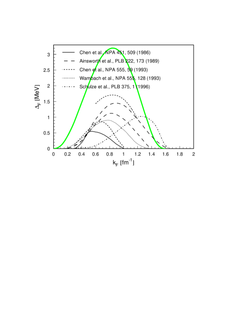
Figure 14: The ${}^{1}S_{0}$ gap in pure neutron matter predicted in several publications taking account of polarization effects. Taken from Lombardo and Schulze (2001)

We conclude by summarizing this section through Fig. 14. This figure exhibits the influence of various approaches which include screening corrections to the pairing gap. The curve in the background is given by the calculation with free single-particle energies and the bare nucleon-nucleon interaction. These calculations are similar, except for the potential model employed, to those discussed in, e.g., Fig. 6. This means that the calculations of Subsec. II.3, with only experimental inputs, phase shifts and scattering length, yield an upper limit for the ${}^{1}S_{0}$ pairing gap. How such renomalizations will affect the ${}^{3}P_{2}$ gap is an entirely open issue. This gap is crucial since it extends to large densities and can reasonably be expected to occur at the centers of neutron stars. Unfortunately, one cannot constrain at present the size of the pairing gap from data on thermal emission from neutron stars, see also the discussion in Sec. II.4.

III PAIRING CORRELATIONS IN FINITE NUCLEI

III.1 Introduction to the nuclear shell model

Our tool for analyzing pairing correlations in finite nuclei is the nuclear shell model, with appropriately defined model spaces and effective interactions. In this section we extract information on pairing correlations through large-scale shell-model calculations of several nuclear systems, from nuclei in the $sd$-shell to heavy tin isotopes.

We define the nuclear shell model by a set of spin-orbit coupled single-particle states with quantum numbers $ljm$ denoting the orbital angular momentum ($l$) and the total angular momenta ($j$) and its $z$-component, $m$. In a rotationally invariant basis, the one-body states have energy $\varepsilon_{lj}$ that are independent of $m$. The single-particle states and energies may be different for neutrons and protons, in which case it is convenient to include also the isospin component $t_{z}=\pm 1/2$ in the state description. We will use the label $\alpha$ for the set of quantum numbers $ljm$ or $ljmt_{z}$, as appropriate. These orbits define the valence $P$-space, or model space for the shell model, while remaining single-particle orbits define the so-called excluded space, or $Q$-space. We can express these spaces through the operators

$$P=\sum_{i=1}^{n}\left|\psi_{i}\right\rangle\left\langle\psi_{i}\right|,\;\;\;Q=\sum_{i=n+1}^{\infty}\left|\psi_{i}\right\rangle\left\langle\psi_{i}\right|,$$ (59)

where $n$ defines the dimension of the model space while the wave functions $\psi_{i}$ could represent a many-body Slater determinant built on the chosen single-particle basis. As an example, if we consider the chain of tin isotopes from ¹⁰⁰Sn to ¹³²Sn, the neutron single-particle orbits $2s_{1/2}$, $1d_{5/2}$, $1d_{3/2}$, $0g_{7/2}$, and $0h_{11/2}$ could define an eventual model space. We could then choose ¹³²Sn as a closed-shell core. Neutron holes from ¹³¹Sn to ¹⁰⁰Sn define then the valence-space or model-space degrees of freedom. We could, however, have chosen ¹⁰⁰Sn as a closed-shell core. In this case, neutron particles from ¹⁰¹Sn to ¹³²Sn define the model space.

The shell-model Hamiltonian $\hat{H}$ is thus built upon such a single-particle basis. The shell-model problem requires normally the solution of a real and symmetric $n\times n$ matrix eigenvalue equation

$$\hat{H}\left|\Psi_{k}\right\rangle=E_{k}\left|\Psi_{k}\right\rangle,$$ (60)

with $k=1,\ldots,n$, where the size of this matrix is defined by the actual shell-model space. The dimensionality $n$ of the eigenvalue matrix $H$ is increasing with an increasing number of valence particles or holes. As an example, for ¹¹⁶Sn with the above mentioned single-particle basis, the dimensionality of the Hamiltonian matrix is of the order of $n\sim 10^{8}$. For nuclei in the rare-earth region, this dimensionality can be of the order of $n\sim 10^{12}-10^{14}$.

The shell-model Hamiltonian can be written in the form $\hat{H}=\hat{H}_{1}+\hat{H}_{2}+\hat{H}_{3}+\dots$ where $\hat{H}_{1}$ is a one-body term typically represented by experimental single-particle energies, see Eq. (32). The two-body term, see Eq. (32), is given in terms of the uncoupled matrix elements $V$ of the two-body interaction. These matrix elements must obey rotational invariance, parity conservation, and (when implemented) isospin invarience. To make explicit the rotational and isospin invariance, we rewrite the two-body Hamiltonian as

$$\hat{H}_{2}=\frac{1}{4}\sum_{\alpha\beta\gamma\delta}\sum_{JT}\left[\left(1+\delta_{\alpha\beta}\right)\left(1+\delta_{\gamma\delta}\right)\right]^{1/2}V_{JT}(\alpha\beta,\gamma\delta)\sum_{MT_{z}}\hat{A}^{\dagger}_{JT;MT_{z}}(\alpha\beta)\hat{A}_{JT;MT_{z}}(\gamma\delta)\;,$$ (61)

where the pair operator is

$$\hat{A}^{\dagger}_{JT;MT_{z}}(\alpha\beta)=\sum_{m_{\alpha},m_{\beta},t_{\alpha},t_{\beta}}\left(j_{\alpha}m_{\alpha}j_{\beta}m_{\beta}\mid JM\right)\left(\frac{1}{2}t_{\alpha}\frac{1}{2}t_{\beta}\mid TT_{z}\right)a^{\dagger}_{j_{\beta}m_{\beta}t_{\beta}}a^{\dagger}_{j_{\alpha}m_{\alpha}t_{\alpha}}\;.$$ (62)

In these expressions $(JM)$ are the coupled angular momentum quantum numbers and $(TT_{z})$ are the coupled isospin quantum numbers. The coupled two-body matrix elements $V_{JT}$ define the valence particle interactions within the given shell-model space. They are matrix elements of a scalar potential $V(\vec{r}_{1},\vec{r}_{2})$ and are defined as

$$\left\langle\left[\psi_{j_{\alpha},t_{\alpha}}(\vec{r}_{1})\times\psi_{j_{\beta},t_{\beta}}(\vec{r}_{2})\right]^{JM;TT_{z}}\mid V(\vec{r}_{1},\vec{r}_{2})\mid\left[\psi_{j_{\delta},t_{\delta}}(\vec{r}_{1})\times\psi_{j_{\gamma},t_{\gamma}}(\vec{r}_{2})\right]^{JM;TT_{z}}\right\rangle\;,$$ (63)

and are independent of $M$ and $T_{z}$. The antisymmetrized matrix elements are $V^{A}_{JT}(\alpha\beta,\gamma\delta)$ and are then given by

$$V^{A}_{JT}(\alpha\beta,\gamma\delta)=\left[\left(1+\delta_{\alpha\beta}\right)\left(1+\delta_{\gamma\delta}\right)\right]^{-1/2}\left[V_{JT}(\alpha\beta,\gamma\delta)-(-1)^{J+j_{a}+j_{b}+T-1}V_{JT}(\beta\alpha,\gamma\delta)\right]\;.$$ (64)

We remark here that three-body or higher-body terms such as $\hat{H}_{3}$ are normally not included in a shell-model effective interaction, although shell-model analyses with three-body interactions have been made in Müther et al. (1985); Engeland et al. (2002).

In the following subsections, we discuss how to extract information about pairing correlations within the framework of large-scale shell-model and shell-model Monte Carlo (SMMC) calculations. In Subsec. III.2, we discuss selected features of the tin isotopes such as the near constancy of the energy difference between the first excited state with $J=2$ and the ground state with $J=0$ for the whole chain of even isotopes from ¹⁰²Sn to ¹³⁰Sn. These are nuclei whose excited states are well reproduced by the neutron model space mentioned above. We relate this near constancy to strong pairing correlations and the same partial waves which contribute to superfluiditity in neutron stars, namely the ${}^{1}S_{0}$ and ${}^{3}P_{2}$ components of the nucleon-nucleon interaction. The ${}^{1}S_{0}$ component is generally the dominating partial wave, a well-known fact in nuclear physics. We show also that a truncation scheme like generalized seniority Talmi (1993) is a viable first approximation to large-scale shell-model calculations.

In Subsec. III.3, we discuss isoscalar and isovector pairing correlations, whereas proton-neutron pairing and Wigner energy are discussed in Subsec. III.4. Various thermal properties are discussed in the remaining subsections. These results are obtained through large-scale SMMC calculations, see for example Koonin et al. (1997).

III.2 Tin isotopes, seniority, and the nucleon-nucleon interaction

Nuclei far from the line of $\beta$-stability are at present in focus of the nuclear structure physics community. Considerable attention is being devoted to the experimental and theoretical study of nuclei near ¹⁰⁰Sn from studies of the chain of Sn isotopes up to ¹³²Sn to, e.g., nuclei near the proton drip line like ^105,106Sb.

Our scheme to obtain an effective two-body interaction for shell-model studies starts with a free nucleon-nucleon interaction $V$, which is appropriate for nuclear physics at low and intermediate energies. Here we employ the charge-dependent version of the Bonn potential models, see Machleidt (2001) and the discussion in Sec. II. The next step in our many-body scheme is to handle the fact that the repulsive core of the nucleon-nucleon potential $V$ is unsuitable for perturbative approaches. This problem is overcome by introducing the reaction matrix $G$, which in a diagrammatic language represents the sum over all ladder types of diagrams. This sum is meant to renormalize the repulsive short-range part of the interaction. The physical interpretation is that the particles must interact with each other an infinite number of times in order to produce a finite interaction. We calculate $G$ using the double-partitioning scheme discussed in Hjorth-Jensen et al. (1995). Since the $G$-matrix represents just the summation to all orders of particle-particle ladder diagrams, there are obviously other terms which need to be included in an effective interaction. Long-range effects represented by core-polarization terms are also needed. In order to achieve this, the $G$-matrix elements are renormalized by the so-called $\hat{Q}$-box method. The $\hat{Q}$-box is made up of non-folded diagrams which are irreducible and valence-linked. Here we include all non-folded diagrams to third order in $G$ Hjorth-Jensen et al. (1995). Based on the $\hat{Q}$-box, we compute an effective interaction $\tilde{H}$ in terms of the $\hat{Q}$-box using the folded-diagram expansion method (see for example Hjorth-Jensen et al. (1995) for further details).

The effective two-particle interaction is then used in large-scale shell-model calculations. For the shell-model calculation, we employ the Oslo $m$-scheme shell-model code Engeland et al. (2002), which is based on the Lanczos algorithm, an iterative method which gives the solution of the lowest eigenstates. The technique is described in detail in Whitehead et al. (1977). The shell-model space consists of the orbits $2s_{1/2}$, $1d_{5/2}$, $1d_{3/2}$, $0g_{7/2}$ and $0h_{11/2}$.

Of interest in this study is the fact that the chain of even tin isotopes from ¹⁰²Sn to ¹³⁰Sn exhibits a near constancy of the $2^{+}_{1}-0^{+}_{1}$ excitation energy, a constancy which can be related to strong pairing correlations and the near degeneracy in energy of the relevant single-particle orbits. As an example, we show the experimental $2^{+}_{1}-0^{+}_{1}$ excitation energy from ¹¹⁶Sn to ¹³⁰Sn in Table 1. Our aim is to see whether partial waves which play a crucial role in superfluidity of neutron star matter, viz. ${}^{1}S_{0}$ and ${}^{3}P_{2}$, are equally important in reproducing the near-constant spacing in the chain of even tin isotopes shown in Table 1.

In order to test whether the ${}^{1}S_{0}$ and ${}^{3}P_{2}$ partial waves are equally important in reproducing the near constant spacing in the chain of even tin isotopes as they are for the superfluid properties of infinite neutron star matter (recall the discussion of Sec. II), we study four different approximations to the shell-model effective interaction, viz.,

1. Our best approach to the effective interaction, $V_{\mathrm{eff}}$, contains all one-body and two-body diagrams through third order in the $G$-matrix, as discussed above, see also Holt et al. (1998).

2. The effective interaction is given by the $G$-matrix only and inludes all partial waves up to $l=10$.

3. We define an effective interaction based on a $G$-matrix which now includes only the ${}^{1}S_{0}$ partial wave.

4. Finally, we use an effective interaction based on a $G$-matrix which does not contain the ${}^{1}S_{0}$ and ${}^{3}P_{2}$ partial waves, but all other waves up to $l=10$.

In all four cases the same NN interaction is used, viz., the CD-Bonn interaction described in Machleidt (2001). Table 1 lists the results.

We note from this table that the three first cases nearly produce a constant $2^{+}_{1}-0^{+}_{1}$ excitation energy, with our most optimal effective interaction $V_{\mathrm{eff}}$ being closest to the experimental data. The bare $G$-matrix interaction, with no folded diagrams as well, results in a slightly more compressed spacing. This is mainly due to the omission of the core-polarization diagrams which typically render the $J=0$ matrix elements more attractive. Such diagrams are included in $V_{\mathrm{eff}}$. Including only the ${}^{1}S_{0}$ partial wave in the construction of the $G$-matrix (case 3) yields, in turn, a somewhat larger spacing. This can again be understood from the fact that a $G$-matrix constructed with this partial wave only does not receive contributions from any entirely repulsive partial wave. It should be noted that our optimal interaction, as demonstrated in Holt et al. (1998), shows a rather good reproduction of the experimental spectra for both even and odd nuclei. Although the approximations made in cases 2 and 3 produce an almost constant $2^{+}_{1}-0^{+}_{1}$ excitation energy, they reproduce poorly the properties of odd nuclei and other excited states in the even Sn isotopes.

However, the fact that the first three approximations result in a such a good reproduction of the $2^{+}_{1}-0^{+}_{1}$ spacing may hint to the fact that the ${}^{1}S_{0}$ partial wave is of paramount importance. If we now turn attention to case 4, i.e., we omit the ${}^{1}S_{0}$ and ${}^{3}P_{2}$ partial waves in the construction of the $G$-matrix, the results presented in Table 1 exhibit a spectroscopic catastrophe. We also do not list eigenstates with other quantum numbers. For ¹²⁶Sn, the ground state is no longer a $0^{+}$ state; rather it carries $J=4^{+}$ while for ¹²⁴Sn the ground state has $6^{+}$. The first $0^{+}$ state for this nucleus is given at an excitation energy of $0.1$ MeV with respect to the $6^{+}$ ground state. The general picture for other eigenstates is that of an extremely poor agreement with data. Since the agreement is so poor, even the qualitative reproduction of the $2^{+}_{1}-0^{+}_{1}$ spacing, we defer from performing time-consuming shell-model calculations for ^{116,118,120,122}Sn.

Since pairing is so prominent in such systems, we present a comparison of the SM with the generalized seniority model Talmi (1993). The generalized seniority scheme is an extension of the seniority scheme, i.e., from involving only one single $j$–orbital, the model is generalized to involve a group of $j$–orbitals within a major shell. The generalized seniority scheme is a more simple model than the shell model since a rather limited number of configurations with a strictly defined structure are included, thus allowing a more direct physical interpretation. States with seniority $v=0$ are by definition states where all particles are coupled in pairs. Seniority $v=2$ states have one pair broken, seniority $v=4$ states have two pairs broken, etc. The generalized seniority scheme is suitable for describing semi-magic nuclei where pairing plays an important role. The pairing picture and the generalized seniority scheme have been important for the description and understanding of the tin isotopes. A typical feature of the seniority scheme is that the spacing of energy levels is independent of the number of valence particles. For the tin isotopes, not only the spacing between the ground state and the $2^{+}_{1}$ state, but also the spacing beween the ground state and the $4^{+}_{1}$ and $6^{+}_{1}$ states is fairly constant throughout the whole sequence of isotopes. In fundamental works on generalized seniority by, for instance, Talmi Talmi (1993), the tin isotopes have been used as one of the major test cases. It is also worth mentioning the classical work on pairing by Kisslinger and Sorensen Kisslinger and Sorensen (1960), see also the analyses of Sandulescu et al. (1997) and the review article of Bes and Sorensen Bes and Sorensen (1969).

If we, by closer investigation and comparison of the SM wave function and the seniority states, find that the most important components are accounted for by the seniority scheme, we can benefit from this and reduce the SM basis. This would be particularly useful when we want to do calculations on systems with a large number of valence particles.

The operator for creating a generalized seniority $(v=0)$ pair is

$$S^{\dagger}=\sum_{j}\frac{1}{\sqrt{2j+1}}\alpha_{j}\sum_{m\geq 0}(-1)^{j-m}b^{\dagger}_{jm}b_{j-m}^{\dagger},$$ (65)

where $b^{\dagger}_{jm}$ is the creation operator for holes. The generalized senitority $(v=2)$ operator for creating a broken pair is given by

$$D_{J,M}^{\dagger}=\sum_{j\leq j^{\prime}}(1+\delta_{j,j^{\prime}})^{-1/2}\beta_{j,j^{\prime}}\langle jmj^{\prime}m^{\prime}\left|JM\right\rangle b^{\dagger}_{jm}b^{\dagger}_{j^{\prime}m^{\prime}}.$$ (66)

The coefficients $\alpha_{j}$ and $\beta_{jj^{\prime}}$ are obtained from the ¹³⁰Sn ground state and the excited states, respectively.

We calculate the squared overlaps between the constructed generalized seniority states and our shell-model states

$$\begin{array}[]{lccccl}(v=0)&&&&&|\langle^{A}{\rm Sn(SM)};0^{+}|(S^{\dagger})^{\frac{n}{2}}|\tilde{0}\rangle|^{2},\\ (v=2)&&&&&|\langle^{A}{\rm Sn(SM)};J_{i}|D^{\dagger}_{JM}(S^{\dagger})^{\frac{n}{2}-1}|\tilde{0}\rangle|^{2}.\end{array}$$ (67)

The vacuum state $|\tilde{0}\rangle$ is the ¹³²Sn–core and $n$ is the number of valence particles. These quantities tell to what extent the shell-model states satisfy the pairing picture, or in other words, how well is generalized seniority conserved as a quantum number.

The squared overlaps are tabulated in Table 2, and vary generally from 0.95 to 0.75. As the number of valence particles increases, the squared overlaps gradually decrease. The overlaps involving the $4^{+}$ states show a fragmentation. In ¹²⁸Sn, the $4^{+}_{1}$ (SM) state is mainly a seniority $v=2$ state. As approaching the middle of the shell, the next state, $4^{+}_{2}$, takes more and more over the structure of a seniority $v=2$ state. The fragmentation of seniority over these two states can be understood from the fact that they are rather close in energy and therefore may have mixed structure.

In summary, these studies show clearly the prominence of pairing correlations in nuclear systems with identical particles as effective degrees of freedom. There is a clear link between superfluidity in infinite neutron star matter and spectra of finite nuclei such as the chain of tin isotopes. This link is provided especially by the ${}^{1}S_{0}$ partial wave of the nucleon-nucleon interaction. Excluding this component from an effective interaction yields spectroscopy in poor agreement with experimental data. Although the ${}^{1}S_{0}$ partial wave plays an important role, other many-body effects arising e.g., from low-lying collective surface vibrations among nucleons can have important effects on properties of nuclei, as demonstrated recently by Broglia et al Barranco et al. (1999); Giovanardi et al. (2002). In order to interpret the results of Table 1 one needs to analyze the core-polarizations diagrams which are used to compute the effective interaction in terms of the various partial waves.

Generalized seniority provides an explicit measure of the degree of pairing correlations in the wave functions. Furthermore, generalized seniority can serve as a useful starting point for large-scale shell-model calculations and is one among several ways of extracting information about pairing correlations. In the next subsections, we present further approaches.

III.3 Isoscalar and isovector pair correlations

Numerous phenomenological descriptions of nuclear collective motion describe the nuclear ground state and its low-lying excitations in terms of bosons. In one such model, the Interacting Boson Model (IBM), $L=0$ (S) and $L=2$ (D) bosons are identified with nucleon pairs having the same quantum numbers Iachello and Arima (1988), and the ground state can be viewed as a condensate of such pairs. Shell-model studies of the pair structure of the ground state and its variation with the number of valence nucleons can therefore shed light on the validity and microscopic foundations of these boson approaches.

Generally speaking, nucleon-nucleon pairing may be considered in several classes. A nucleon has a spin $j=1/2,j_{z}=\pm 1/2$ and an isospin $t=1/2,t_{z}=\pm 1/2$. Two protons (neutrons) thus are allowed to become paired to total $J,T=0,1$ and $T_{z}=-1$ ($T_{z}=1$). We shall call this isovector pairing. Isoscalar pairing delineates proton-neutron pairing for which $J,T=1,0$ and $T_{z}=0$.

While we concentrate here on shell model results, we do wish to point out to the reader several recent developments in other model studies of nucleon-nucleon pairing. Interesting studies of nucleon-nucleon pairing have been undertaken in several models, including pseudo-$SU(4)$ symmetry studies for $pf$-shell nuclei Van Isacker et al. (1999). These studies indicated that pseudo-$SU(4)$ is a reasonable starting point for the description of systems within the $pf$-shell larger than ⁵⁶Ni. It is also the starting point for generating collective pairs within the framework of the Interacting Boson Model that incorporates $T=0$ and $T=1$ bosons and a bosonic $SU(4)$ algebra Elliott (1958). This symmetry dictates that pairing strengths are the same in the both the $T=0$ and $T=1$ channels. Extensive studies of pairing in the framework of Hartree-Fock-Bogoliubov theory have also been undertaken (see, for example Goodman (2000)). Recent work in this direction indicates that $T=0$ and $T=1$ pairing superfluids may develop near the mid-point of isotope chains (i.e., near $N=Z$ nuclei).

In the framework of the shell model, it appears sufficient for many purposes to study the BCS pair structure in the ground state. The BCS pair operator for protons can be defined as

$$\hat{\Delta}^{\dagger}_{p}=\sum_{jm>0}p^{\dagger}_{jm}p^{\dagger}_{j\bar{m}}\;,$$ (68)

where the sum is over all orbitals with $m>0$ and $p^{\dagger}_{j\bar{m}}=(-)^{j-m}p^{\dagger}_{jm}$ is the time-reversed operator. Thus, the observable $\hat{\Delta}^{\dagger}\hat{\Delta}$ and its analog for neutrons are measures of the numbers of $J=0,T=1$ pairs in the ground state. For an uncorrelated Fermi gas, we have simply

$$\langle\hat{\Delta}^{\dagger}\hat{\Delta}\rangle=\sum_{j}{n_{j}^{2}\over{2(2j+1)}},$$ (69)

where the $n_{j}=\langle p^{\dagger}_{jm}p_{jm}\rangle$ are the occupation numbers, so that any excess of $\langle\hat{\Delta}^{\dagger}\hat{\Delta}\rangle$ in our SMMC calculations over the Fermi-gas value indicates pairing correlations in the ground state.

In this analysis, we move from tin isotopes to nuclei which can be described by the single-particle orbits of the $pf$-shell, $1p_{3/2}$, $1p_{1/2}$, $0f_{5/2}$, and $0f_{7/2}$. As effective interaction, we employ the phenomenological interaction of Brown and Richter Richter et al. (1991). Fig. 15 shows the SMMC expectation values of the proton and neutron BCS-like pairs, obtained after subtraction of the Fermi gas value (Eq. 69), for three chains of isotopes. As expected, these excess pair correlations are quite strong and reflect the well-known coherence in the ground states of even-even nuclei. Note that the proton BCS-like pairing fields are not constant within an isotope chain, showing that there are important proton-neutron correlations present in the ground state. The shell closure at $N=28$ is manifest in the neutron BCS-like pairing. As is demonstrated in Fig. 16, the proton and neutron occupation numbers show a much smoother behavior with increasing $A$.

It should be noted that the BCS form (Eq. 68) in which all time-reversed pairs have equal amplitude is not necessarily the optimal one and allows only the study of S-pair structure. To explore the pair content of the ground state in a more general way Alhassid et al. (1996); Langanke et al. (1996), we define proton pair creation operators

$$\hat{A}^{\dagger}_{J\mu}(j_{a}j_{b})={1\over\sqrt{1+\delta_{ab}}}[a^{\dagger}_{j_{a}}\times a^{\dagger}_{j_{b}}]_{J\mu}\;.$$ (70)

These operators are boson-like in the sense that

$$[\hat{A}^{\dagger}_{J\mu}(j_{a}j_{b}),\hat{A}_{J\mu}(j_{a}j_{b})]=1+{\cal O}(\hat{n}/2j+1)\;;$$ (71)

i.e., they satisfy the expected commutation relations in the limit of an empty shell. We may also construct from these operators a pair matrix

$$M^{J}_{\alpha\alpha^{\prime}}=\frac{1}{\sqrt{2(1+\delta_{j_{a}j_{b}})}}\sum_{M}\langle A^{\dagger}_{JM}(j_{a},j_{b})A_{JM}(j_{c},j_{d})\rangle$$ (72)

We construct bosons $\hat{B}^{\dagger}_{\alpha J\mu}$ as

$$\hat{B}^{\dagger}_{\alpha J\mu}=\sum_{j_{a}j_{b}}\psi_{\alpha\lambda}(j_{a}j_{b})\hat{A}^{\dagger}_{\lambda\mu}(j_{a}j_{b})\;,$$ (73)

where $\alpha=1,2,\ldots$ labels the particular boson and the “wave function” $\psi$ satisfies

$$\sum_{j_{a}j_{b}}\psi^{\ast}_{\alpha J}(j_{a}j_{b})\psi_{\beta J}(j_{a}j_{b})=\delta_{\alpha\beta}\;.$$ (74)

(Note that $\psi$ is independent of $\mu$ by rotational invariance.)

To find $\psi$ and $n_{\alpha J}\equiv\sum_{\mu}\langle\hat{B}^{\dagger}_{\alpha J\mu}\hat{B}_{\alpha J\mu}\rangle$, the number of bosons of type $\alpha$, and multipolarity $J$, we compute the quantity $\sum_{\mu}\langle\hat{A}^{\dagger}_{J\mu}(j_{a}j_{b})\hat{A}_{J\mu}(j_{c}j_{d})\rangle$, which can be thought of as an hermitian matrix $M^{J}_{\alpha\alpha^{\prime}}$ in the space of orbital pairs $(j_{a}j_{b})$; its non-negative eigenvalues define the $n_{\alpha J}$ (we order them so that $n_{1J}>n_{2J}>\ldots$), while the normalized eigenvectors are the $\psi_{\alpha J}(j_{a}j_{b})$. The index $\alpha$ distinguishes the various possible bosons. For example, in the complete $pf$-shell the square matrix $M$ has dimension $N_{J}=4$ for $J=0$, $N_{J}=10$ for $J=1$, $N_{J}=13$ for $J=2,3$.

The presence of a pair condensate in a correlated ground state will be signaled by the largest eigenvalue for a given $J$, $n_{1J}$, being much greater than any of the others; $\psi_{1J}$ will then be the condensate wavefunction. In Fig. 17 we show the pair matrix eigenvalues $n_{\alpha J}$ for the three isovector $J=0^{+}$ pairing channels as calculated for the iron isotopes ^54-58Fe. We compare the SMMC results with those of an uncorrelated Fermi gas, where we can compute $\langle\hat{A}^{\dagger}\hat{A}\rangle$ using the factorization

$$\langle a^{\dagger}_{\alpha}a^{\dagger}_{\beta}a_{\gamma}a_{\delta}\rangle=n_{\beta}n_{\alpha}(\delta_{\beta\gamma}\delta_{\alpha\delta}-\delta_{\beta\delta}\delta_{\alpha\gamma})\;,$$ (75)

where the $n_{\beta}=\langle a^{\dagger}_{\beta}a_{\beta}\rangle$ are the occupation numbers. Additionally, Fig. 17 shows the diagonal matrix elements of the pair matrix $M_{\alpha\alpha}$. As expected, the protons occupy mainly $f_{7/2}$ orbitals in these nuclei. Correspondingly, the $\langle\hat{A}^{\dagger}\hat{A}\rangle$ expectation value is large for this orbital and small otherwise. For neutrons, the pair matrix is also largest for the $f_{7/2}$ orbital. The excess neutrons in ^56,58Fe occupy the $p_{3/2}$ orbital, signaled by a strong increase of the corresponding pair matrix element $M_{22}$ in comparison to its value for ⁵⁴Fe. Upon closer inspection, we find that the proton pair matrix elements are not constant within the isotope chain. This behavior is mainly caused by the isoscalar proton-neutron, pairing. The dominant role is played by the isoscalar $1^{+}$ channel, which couples protons and neutrons in the same orbitals and in spin-orbit partners. As a consequence we find that, for ^54,56Fe, the proton pair matrix in the $f_{5/2}$ orbital, $M_{33}$, is larger than in the $p_{3/2}$ orbital, although the latter is favored in energy. For ⁵⁸Fe, this ordering is inverted, as the increasing number of neutrons in the $p_{3/2}$ orbital increases the proton pairing in that orbital.

After diagonalization of $M$, the $J=0$ proton pairing strength is essentially found in one large eigenvalue. Furthermore, we observe that this eigenvalue is significantly larger than the largest eigenvalue on the mean-field level (Fermi gas), supporting the existence of a proton pair condensate in the ground state of these nuclei. The situation is somewhat different for neutrons. For ⁵⁴Fe, only little additional coherence is found beyond the mean-field value, reflecting the closed-subshell neutron structure. For the two other isotopes, the neutron pairing exhibits two large eigenvalues. Although the larger one exceeds the mean-field value and signals noticeable additional coherence across the subshells, the existence of a second coherent eigenvalue shows the shortcomings of the BCS-like pairing picture.

It has long been anticipated that $J=0^{+}$ proton-neutron correlations play an important role in the ground states of $N=Z$ nuclei. To explore these correlations, we have performed SMMC calculations of the $N=Z$ nuclei in the mass region $A=48-56$ Langanke et al. (1997a). Note that for these nuclei the pair matrix in all three isovector $0^{+}$ channels essentially exhibits only one large eigenvalue, related to the $f_{7/2}$ orbital. We will use this eigenvalue as a convenient measure of the pairing strength. As the even-even $N=Z$ nuclei have isospin $T=0$, the expectation values of ${\hat{A}}^{\dagger}{\hat{A}}$ are identical in all three isovector $0^{+}$ pairing channels. This symmetry does not hold for the odd-odd $N=Z$ nuclei in this mass range, which have $T=1$ ground states, and $\langle\hat{A}^{\dagger}\hat{A}\rangle$ can be different for proton-neutron pairs than for like-nucleons pair (the expectation values for proton pairs and neutron pairs are identical). We find the proton-neutron pairing strength significantly larger for odd-odd $N=Z$ nuclei than in even-even nuclei, while the $0^{+}$ proton and neutron pairing shows the opposite behavior, in both cases leading to an odd-even staggering, as displayed in Fig. 18. This staggering is caused by a constructive interference of the isotensor and isoscalar parts of $\hat{A}^{\dagger}\hat{A}$ in the odd-odd $N=Z$ nuclei, while they interfere destructively in the even-even nuclei. The isoscalar part is related to the pairing energy, and is found to be about constant for the nuclei studied here. Similar behavior was also demonstrated in a simplified $SO(5)$ seniority-like model Engel et al. (1996, 1998). This model is analytic, but shows the same trends as the shell model results. Due to other correlations present in the shell model, such as the inclusion of several orbits, isoscalar pairing, spin-orbit splitting, long-range correlations, deformation, etc., the shell model results are reduced in comparison to the simplified model. Pairing correlations have also been studied in heavier systems that require the presence of the $0g_{9/2}$ orbital Dean et al. (1997); Petrovici et al. (2000). In heavier odd-odd $N=Z$ nuclei the ground state becomes a $T=1$ (rather than $T=0$), as was found experimentally in ⁷⁴Rb Rudolph and et al (1996). The lowest $T=0$ and $T=1$ states in these systems are very close in energy. Recently, mean-field calculations that include both $T=0$ and $T=1$ pairing correlations in odd-odd $N=Z$ nuclei Satula and Wyss (2001) showed that the interplay between quasiparticle excitations (relevant for the case of $T=0$ states) and isorotations (relevant for the case of $T=1$ states) explains the near degeneracy of these states.

III.4 Proton-neutron pairing and the Wigner energy

So far, the strongest evidence for $np$ pairing comes from the masses of $N$=$Z$ nuclei. An additional binding (the so-called Wigner energy) found in these nuclei manifests itself as a spike in the isobaric mass parabola as a function of $T_{z}$=$\frac{1}{2}(N-Z)$ (see the review Zeldes (1996) and references quoted therein). Gross estimates of the magnitude of the Wigner energy come from a large-scale fit to experimental binding energies with the macroscopic-microscopic approach Myers and Swiatecki (1966); Krappe et al. (1979) and from the analysis of experimental masses Jensen et al. (1984). Several early attempts were made to incorporate the effect of neutron-proton pair correlations in light nuclei in quasiparticle theory (for an early review see Goodman (1979)) with varying success. Satula et al, Satula et al. (1997) presented a technique to extract the Wigner energy directly from the experimental data and gave empirical arguments that this energy originates primarily from the $T$=0 part of the effective interaction. To obtain deeper insight into the structure of the Wigner term, they applied the nuclear shell model to nuclei from the $sd$ and $fp$ shells.

The Wigner energy, $E_{W}$, is believed to represent the energy of collective $np$-pairing correlations. It enters the semi-empirical mass formula (see e.g. Krappe et al. (1979)) as an additional binding due to the $np$-pair correlations. The Wigner energy can be decomposed into two parts:

$$E_{W}=W(A)|N-Z|+d(A)\pi_{np}\delta_{NZ},$$ (76)

The $|N-Z|$-dependence in Eq. (76) was first introduced by Wigner Wigner (1937) in his analysis of the SU(4) spin-isospin symmetry of nuclear forces. In the supermultiplet approximation, there appears a term in the nuclear mass formula which is proportional to $T_{\rm gs}(T_{\rm gs}+4)$, where $T_{\rm gs}$ denotes the isospin of the ground state. Empirically, $T_{\rm gs}$=$|T_{z}|$ for most nuclei except for heavy odd-odd $N$=$Z$ systems Jänecke (1965); Zeldes and Liran (1976). Although the experimental data indicate that the SU(4) symmetry is severely broken, and the masses behave according to the $T_{\rm gs}(T_{\rm gs}+1)$ dependence Jänecke (1965); Jensen et al. (1984), the expression of Eq. (76) for the Wigner energy is still very useful. In particular, it accounts for a non-analytic behavior of nuclear masses when an isobaric chain crosses the $N$=$Z$ line. An additional contribution to the Wigner term, the $d$-term in Eq. (76), represents a correction for $N$=$Z$ odd-odd nuclei. Theoretical justification of Eq. (76) has been given in terms of basic properties of effective shell-model interactions Zeldes (1996); Talmi (1962), and also by using simple arguments based on the number of valence $np$-pairs Jensen et al. (1984); Myers (1977). The estimates based on the number of $np$ pairs in identical spatial orbits suggest that the ratio $d/W$ is constant and equal to one Myers (1977). A different estimate has been given in Jensen et al. (1984): $d/W$=0.56$\pm$0.27.

In the work of Satula Satula et al. (1997), the Wigner energy coefficient $W$ in an even-even nucleus $Z$=$N$=$\frac{A}{2}$ was extracted by means of the indicator:

$$W(A)=\delta V_{np}\left(\frac{A}{2},\frac{A}{2}\right)-{1\over 2}\left[\delta V_{np}\left(\frac{A}{2},\frac{A}{2}-2\right)+\delta V_{np}\left(\frac{A}{2}+2,\frac{A}{2}\right)\right].$$ (77)

The $d$-term in an odd-odd nucleus, $Z$=$N$=$\frac{A}{2}$ [Eq. (76)], can be extracted using another indicator:

$$d(A)=2\left[\delta V_{np}\left(\frac{A}{2},\frac{A}{2}-2\right)+\delta V_{np}\left(\frac{A}{2}+2,\frac{A}{2}\right)\right]-4\delta V_{np}\left(\frac{A}{2}+1,\frac{A}{2}-1\right)\;,$$ (78)

where the double-difference formula from Zhang et al. (1989) is

$$\delta V_{np}(N,Z) = {1\over 4}\left\{B(N,Z)-B(N-2,Z)-B(N,Z-2)+B(N-2,Z-2)\right\}$$ (79)

$$\approx {\partial^{2}B\over{\partial N\partial Z}}.$$

Although the recipe for these third-order mass difference indicators is not unique, the results appear to be very weakly dependent on the particular prescription used.

To visualize the influence of the $T$=0 part of the effective nuclear interaction on the Wigner term, we have performed a set of shell-model calculations while switching off sequentially the $J=1,2,...,J_{\rm max}$, $T$=0 two-body matrix elements $\langle j_{1}j_{2}JT|\hat{H}|j_{1}^{\prime}j_{2}^{\prime}JT\rangle$ of the shell-model Hamiltonian $\hat{H}$ for different values of $J_{\rm max}$. Figure 19 shows a ratio $\varepsilon_{W}/\varepsilon_{W}^{\rm total}$, where $\varepsilon_{W}^{\rm total}$ denotes the result of full shell-model calculations versus $J_{\rm max}$. The calculations were performed for two representative examples, namely, the $fp$-shell nucleus ⁴⁸Cr and the $sd$-shell nucleus ²⁴Mg. The largest contribution to the Wigner energy comes from the part of the $T$=0 interaction between deuteron-like ($J$=1) and ‘stretched’ [$J$=5 ($sd$) and 7 ($pf$)] pairs. The importance of these matrix elements is well known; it is precisely for $J$=1 and stretched pair-states that experimentally determined effective $np$ $T$=0 interactions are strongest Anataraman and Schiffer (1971); Schiffer (1971); Molinari et al. (1975). Note also that the deuteron-like correlations contribute more strongly to $\varepsilon_{W}$ in $sd$-nuclei than in $fp$-nuclei, and that matrix elements corresponding to intermediate values of $J$ give non-negligible contributions. This reveals the complex structure of the Wigner energy and suggests that models which ignore high-$J$ components of the $np$ interaction (e.g., by considering only $J$=0, $T$=1 and $J$=1, $T$=0 $np$ pairs Evans et al. (1981)) are not too useful for discussing the actual $np$ pair correlations.

III.5 Thermal properties of $pf$-shell nuclei

The properties of nuclei at finite temperatures are of considerable experimental (for reviews, see Suraud et al. (1989); Snover (1986)) and theoretical interest Alhassid (1991); Egido and Ring (1993). How thermal excitations influence the pairing properties will be the main focus of this section. We address this topic in Sec. V as well but with an emphasis on an analysis based on experimental data on level densities.

Theoretical studies of nuclei at finite temperature have been based mainly on mean-field approaches and thus only consider the temperature dependence of the most probable configuration in a given system. These approaches have been criticized due to their neglect of quantum and statistical fluctuations Dukelsky et al. (1991). The SMMC method does not suffer this defect and allows the consideration of model spaces large enough to account for the relevant nucleon-nucleon correlations at low and moderate temperatures.

SMMC calculations were performed to study the thermal properties of several even-even and odd-A nuclei in the mass region $A=50-60$ Dean et al. (1994); Langanke et al. (1996) in an $fp$-shell model space using realistic interactions. More recently, Alhassid et al., carried out thermal calculations in a larger model-space which included the $0g_{9/2}$ shell. As a typical example, we discuss in the following our SMMC results for the nucleus ⁵⁴Fe, which is very abundant in the presupernova core of a massive star.

Our calculations include the complete set of $1p_{3/2,1/2}0f_{7/2,5/2}$ states interacting through the realistic Brown-Richter Hamiltonian Richter et al. (1991). (SMMC calculations using the modified KB3 interaction Poves and Zuker (1981a, b) give essentially the same results.) Some $5\times 10^{9}$ configurations of the 8 valence neutrons and 6 valence protons moving in these 20 orbitals are involved in the canonical ensemble. The results presented below have been obtained with a time step of $\Delta\beta=1/32~{}{\rm MeV}^{-1}$ using 5000–9000 independent Monte Carlo samples.

The calculated temperature dependence of various observables is shown in Fig. 20. In accord with general thermodynamic principles, the internal energy $U$ steadily increases with increasing temperature Dean et al. (1994). It shows an inflection point around $T\approx 1.1$ MeV, leading to a peak in the heat capacity, $C\equiv dU/dT$, whose physical origin we will discuss below. The decrease in $C$ for $T\gtrsim 1.4$ MeV is due to our finite model space (the Schottky effect Civitarese et al. (1989)); we estimate that limitation of the model space to only the $pf$-shell renders our calculations of ⁵⁴Fe quantitatively unreliable for temperatures above this value (internal energies $U\gtrsim 15$ MeV). The same behavior is apparent in the level density parameter, $a\equiv C/2T$. The empirical value for $a$ is $A/8~{}{\rm MeV}=6.8~{}{\rm MeV}^{-1}$, which is in good agreement with our results for $T\approx 1.1$–1.5 MeV.

More recent calculations confirm these basic findings. Liu and Alhassid calculated Liu and Alhassid (2001) the heat capacity for iron isotopes in a complete $0f1p-g_{9/2}$ model space. They used a phenomenological pairing-plus-quadrupole model for the two-body interaction and found that the pairing transition in the heat capacity is correlated with the suppression of the number of spin-zero neutron pairs as the temperature increases. The results were obtained using a novel method to calculate the heat capacity that decrease the statistical error bars in the calculation. We show results of this calculation for Fe isotopes in Fig. 21. While the original calculations of Dean et al. (1994) indicate a possible phase transition (along with a pairing collapse in the measured $\langle\Delta^{\dagger}\Delta\rangle$ pairing expectation), this effect appears to be delayed to more neutron-rich nuclei in the calculations of Liu and Alhassid (2001). Several factors likely contribute to this difference. First, the interactions are obviously different. Second, the extrapolation techniques used for realistic interactions likely over-estimate the influence of pairing in the region between $0.5$ and 1.0 MeV. Finally, the model space is smaller in the early calculation, although the Schottky peak is seen to appear at about 1.4 MeV. This makes the interpretation of the low temperature peak more difficult in Dean et al. (1994). Nevertheless, it should be clear that both the original calculations with realistic interactions and the more recent work in Liu and Alhassid (2001) both indicate interesting physics related to pairing phenomena in the $T=1.0$ MeV region.

We also show in Fig. 20 the expectation values of the BCS-like proton-proton and neutron-neutron pairing fields, $\langle\hat{\Delta}^{\dagger}\hat{\Delta}\rangle$. At low temperatures, the pairing fields are significantly larger than those calculated for a non-interacting Fermi gas, indicating a strong coherence in the ground state. With increasing temperature, the pairing fields decrease, and both approach the Fermi gas values for $T\approx 1.5$ MeV and follow it closely for even higher temperatures. Associated with the breaking of pairs is a dramatic increase in the moment of inertia, $I\equiv\langle J^{2}\rangle/3T$, for $T=1.0$–1.5 MeV; this is analogous to the rapid increase in magnetic susceptibility in a superconductor. At temperatures above 1.5 MeV, $I$ is in agreement with the rigid rotor value, $10.7\hbar^{2}$/MeV; at even higher temperatures, it decreases linearly due to our finite model space.

Although the results discussed above are typical for even-even nuclei in this mass region (including the $N=Z$ nucleus ⁵²Fe), they are not for odd-odd $N=Z$ nuclei. This is illustrated in Fig. 22 which shows the thermal behavior of several observables for ⁵⁰Mn ($N=Z=25$), calculated in a SMMC study within the complete $pf$-shell using the KB3 interaction Poves and Zuker (1981a, b). A closer inspection of the isovector $J=0$ and isoscalar $J=1$ pairing correlations holds the key to the understanding of these differences. The $J=0$ isovector correlations are studied using the BCS pair operators, Eq. (68) with a similar definition for proton-neutron pairing. For the isoscalar $J=1$ correlations, we have interpreted the trace of the pair matrix $M^{J=1}$ (defined in Eq.  (72)) as an overall measure for the pairing strength,

$$P_{sm}^{J}=\sum_{\beta}\lambda_{\beta}^{J}=\sum_{\alpha}M^{J}_{\alpha\alpha}.$$ (80)

Note that at the level of the non-interacting Fermi gas, proton-proton, neutron-neutron, and proton-neutron $J=0$ correlations are identical for $N=Z$ nuclei. However, the residual interaction breaks the symmetry between like-pair correlations and proton-neutron correlations in odd-odd $N=Z$ nuclei. As is obvious from Fig. 22, at low temperatures proton-neutron pairing dominates in ⁵⁰Mn, while pairing among like nucleons shows only a small excess over the Fermi gas values, in strong contrast to even-even nuclei.

A striking feature of Fig. 22 is that the isovector proton-neutron correlations decrease strongly with temperature and have essentially vanished at $T=1$ MeV, while the isoscalar pairing strength remains about constant in this temperature region (as it does in even-even nuclei) and greatly exceeds the Fermi gas values. We also note that the pairing between like nucleons is roughly constant at $T<1$ MeV. The change of importance between isovector and isoscalar proton-neutron correlations with temperature is nicely reflected in the isospin expectation value, which decreases from $<\hat{T}^{2}>=2$ at temperatures around 0.5 MeV, corresponding to the dominance of isovector correlations, to $<\hat{T}^{2}>=0$ at temperature $T=1$ MeV, when isoscalar proton-neutron correlations are most important.

The temperature dependence of the excitation energy $E=\langle H\rangle$ in the odd-odd nucleus ⁵⁰Mn is significantly different than that in even-even nuclei. The difference is due to the uniqueness of isospin properties in odd-odd $N=Z$ nuclei. It is only in these nuclei that one finds states of different isospin, $T=1$ and $T=0$, that are close to each other at low excitation energies. The ⁵⁰Mn ground state is $T=1$, $T_{z}=0$, and $J^{\pi}=0^{+}$. In that state $pn$ pair correlations dominate, and the like-particle correlations are reduced Langanke et al. (1997a). However, at relatively low excitation energy these nuclei exhibit a multiplet of $T=0$ states with nonvanishing angular momenta. These states contribute efficiently to corresponding thermal averages. On the other hand, it follows from isospin symmetry that in the $T=0$ states all three pairing strengths (in $T_{Z}$) must be equal. Thus, at temperatures where the $T=0$ states dominate the thermal average, the $pn$ pair correlations are substantially reduced when compared to ground state values. This argument appears to be a generic feature of odd-odd $N=Z$ nuclei beyond ⁴⁰Ca. For a further discussion see Langanke et al. (1997b). For a different point of view from the perspective of mean-field calculations, see, for example Röpke et al. (2000).

III.6 Pair correlations and thermal response

All SMMC calculations of even-even nuclei in the mass region $A=50-60$ show that the BCS-like pairs break at temperatures around 1 MeV. Three observables exhibit a particularly interesting behavior at this phase transition: a) the moment of inertia rises sharply; b) the M1 strength shows a sharp rise, but unquenches only partially; and c) the Gamow-Teller strength remains roughly constant (and strongly quenched). Note that the $B(M1)$ and $B(GT_{+})$ strengths unquench at temperatures larger than $\approx 2.6$ MeV and in the high-temperature limit approach the appropriate values for our adopted model space.

Langanke et al. (1996) has studied the pair correlations in the four nuclei ^54-58Fe and ⁵⁶Cr for the various isovector and isoscalar pairs up to $J=4$, tentatively interpreting the sum of the eigenvalues of the matrix $M^{J}$ 72 as an overall measure for the pairing strength. Note that the pairing strength, as defined in 80, is non-zero at the mean-field level. The physically relevant pair correlations $P_{\rm corr}^{J}$ are then defined as the difference of the SMMC and mean-field pairing strengths.

Detailed calculations of the pair correlations have been performed for selected temperatures in the region between $T=0.5$ MeV and 8 MeV. Fig. 23 shows the temperature dependence of those pair correlations that play an important role in understanding the thermal behavior of the moment of inertia and the total $M1$ and Gamow-Teller strengths.

The most interesting behavior is found in the $J=0$ proton and neutron pairs. There is a large excess of this pairing at low temperatures, reflecting the ground state coherence of even-even nuclei. With increasing temperature, this excess diminishes and vanishes at around $T=1.2$ MeV. We observe further from Fig. 23 that the temperature dependence of the $J=0$ proton-pair correlations are remarkably independent of the nucleus, while the neutron pair correlations show interesting differences. At first, the correlation excess is smaller in the semimagic nucleus ⁵⁴Fe than in the others. When comparing the iron isotopes, the vanishing of the neutron $J=0$ correlations occurs at higher temperatures with increasing neutron number.

The vanishing of the $J=0$ proton and neutron pair correlations is accompanied by an increase in the correlations of the other pairs. For example, the isovector $J=0$ proton-neutron correlations increase by about a factor of 3 after the $J=0$ proton and neutron pairs have vanished. The correlation peak is reached at higher temperatures with increasing neutron number, while the peak height decreases with neutron excess.

The isoscalar proton-neutron $J=1$ pairs show an interesting temperature dependence. At low temperatures, when the nucleus is still dominated by the $J=0$ proton and neutron pairs, the isoscalar proton-neutron correlations show a noticeable excess but, more interestingly, they are roughly constant and do not directly reflect the vanishing of the $J=0$ proton and neutron pairs. However, at $T>1$ MeV, where the $J=0$ proton- and neutron-pairs have broken, the isoscalar $J=1$ pair correlations significantly increase and have their maximum at around 2 MeV, with peak values of about twice the correlation excess in the ground state. In contrast to the isovector $J=0$ proton-neutron pairs, the correlation peaks occur at lower temperatures with increasing neutron excess. We also observe that these correlations fade rather slowly with increasing temperature.

A further discussion on thermal properties through recent experimental information on level densities will be given in Sec. V.

IV RANDOM INTERACTIONS AND PAIRING

We have seen that all even-even nuclei have a $J^{\pi}=0^{+}$ ground state. Pairing in even-even systems was also shown in previous sections to be a major contributor to the ground-state correlations. Furthermore, a property like the $0^{+}$ nature of all even nuclei can be explained within the simple seniority model, based itself on the short-range nature of the effective interaction. It is therefore interesting to see whether such a general property is specific of this hamiltonian or whether it could also emerge from a random ensemble of rotationally and isospin invariant random two-body interactions. This question was first posed in Johnson et al. (1998), where the low-lying spectral properties of random interactions were first studied from the shell-model perspective. Several interesting results were obtained including highly likely $0^{+}$ ground states emerging from the random ensembles, an enhanced phonon collectivity, strongly correlated pairing phenomena Johnson et al. (2000), odd-even staggering Papenbrock et al. (2002), and a likelihood of generating rotational and vibrational spectra.

Similar results were also obtained in the interacting boson model (IBM) Bijker and Frank (2000). The IBM Hamiltonian used in these calculations is given by

$$H = \epsilon\hat{n}_{d}-\kappa\hat{Q}(\chi)\times\hat{Q}(\chi)\;$$ (81)

$$\hat{Q}_{\mu}(\chi) = \left(s^{\dagger}\tilde{d}+d^{\dagger}s\right)_{\mu}^{(2)}+\chi\left(d^{\dagger}\tilde{d}\right)^{(2)}_{\mu}\;,$$ (82)

where only spin 0 ($s$, monopole) and spin 2 ($d$, quadrupole) bosons are considered. This interaction is randomized by introducing a scaling parameter $\eta=\epsilon/\left[\epsilon+4\kappa(N-1)\right]$ and $\bar{\chi}=2\chi/\sqrt{7}$, and choosing $\bar{\chi}$ and $\eta$ randomly on the intervals $[-1,1]$ and $[0,1]$, respectively. The IBM calculations also gave a predominance of $0^{+}$ ground states as well as strong evidence for the occurence of both vibrational and rotational band structures. Within the shell model, these structures appear within a continuum of rotational bands, but the nature of the IBM model restricts the structures to be of these two particular forms. In this section we will briefly review the present status of research into this interesting phenomena.

For fermions, we define the two-body matrix elements $V_{JT}(ab,cd)$ through an ensemble of two-particle Hamiltonians and require that the ensemble be invariant under changes in the basis of two-particle states. This is achieved by taking the matrix elements to be Gaussian distributed about zero with the widths possibly depending on $J$ and $T$ such that:

$$\matrix{\displaystyle\langle V_{\alpha,\alpha^{\prime}}^{2}\rangle=c_{J_{\alpha},T_{\alpha}}(1+\delta_{\alpha,\alpha^{\prime}})\bar{v}^{2},\hfill\cr\vskip 12.50002pt\cr\displaystyle\langle V_{\alpha,\alpha^{\prime}}V_{\beta,\beta^{\prime}}\rangle=0,\,\,\,(\alpha,\alpha^{\prime})\neq(\beta,\beta^{\prime}).\hfill\cr}$$ (83)

Here $\bar{v}$ is an overall energy scale that we generally ignore (except for scaling single-particle energies for the RQE-SPE defined below). The coefficients $c_{J}$ then define the ensemble. We emphasize that $J,T$ refer to quantum numbers of two-body states and not of the final many-body states (typically 4-10 valence particles).

Several basic ensembles may be defined by the choice of the form of the $c_{J,T}$ coefficients and the single-particle Hamiltonian, if present. One ensemble is called the Random Quasiparticle Ensemble (RQE). In this case $c_{J,T}=\left[(2T+1)(2J+1)\right]^{-1}$. This relation between the $c_{J,T}$, which was discussed in Johnson et al. (1998), came from imposing on the ensemble the constraint that it should remain the same for the particle-particle interaction as for the particle-hole interaction. A different ensemble in this class is called the two-body random ensemble (TBRE) for which $c_{JT}=$ constant. Historically, this was the first two-particle random ensemble to be employed in studying statistical properties of many-particle spectra French and Wong (1970). These two ensembles assume degenerate single-particle energies. Realistic interactions do have nondegenerate single-particle energies that will, in principle, affect various spectral properties. For calculations in the sd shell one uses single-particle energies from the Wildenthal interaction Wildenthal (1984a), scaling $\bar{v}=3.84$ MeV to best match the widths of the two-particle matrix elements. The resulting interactions with the single-particle splitting included are called the RQE-SPE and TBRE-SPE.

The first, and perhaps most striking, feature of all of these random interactions is the preponderance of $J^{\pi}=0+$ ground states. In Fig. 24 we show the distribution of ground-state spins in the various ensembles for the two systems ²⁰Ne and ²⁴Mg. We generated 1000 random interactions from each ensemble. These results are typical and consistent with calculations with only one type of particle (for example, neutrons only), or fermions in which the $\vec{l}\cdot\vec{s}$ force is not present Kaplan et al. (2001).

Fig. 24 also shows that the even spins are preferred. In some cases, higher even spin states are preferred over medium spin states. For example, in ²⁴Mg, the $8^{+}$ state is preferred over the $6^{+}$. The single-particle splitting tends to lower slightly the number of $0^{+}$ ground states. The RQE clearly obtains the highest number of $0^{+}$ ground states in each case.

Various research efforts have been undertaken to understand the preponderance of the $0^{+}$ ground-state. Ensembles of interactions derived from a Gaussian unitary ensemble (GUE) distribution are not time-reversal invariant, but both the Gaussian orthogonal ensemble (GOE) and GUE random ensembles yield $0^{+}$ dominance Bijker et al. (1999). This apparent paradox was recently resolved Velazques and Zuker (2002) by noting that the $J^{2}$ operator commutes with the ${\cal T}$ time-reversal operator for either ensemble. For bosons, Kusnezov Kusnezov (2000) was able to map the $U(4)$ vibron model onto random polynomials on the unit interval. Kusnezov was then able to show analytically the origin of $0^{+}$ ground states. While the $U(4)$ model is extremely simplified and only describes bosons (rather than fermions), it points to the interesting link between random polynomials and the two-body interaction. The $0^{+}$ predominance in the fermion case was recently studied by Mulhall et al Mulhall et al. (2000). These authors used a single $j$-shell to show that statistical correlations of fermions in a finite system with random interactions drive the ground state spin to its minimum or maximum value. The effect is universal and related to the geometric chaoticity, or the assumption of pseudorandom coupling of angular momentum Zelevinsky et al. (1996), of the spin coupling of individual fermions. While a rigorous derivation of these findings for general orbital schemes is not yet available, the research is pointing towards an understanding of why an ensemble of random interactions posesses predominantly $0^{+}$ ground states.

A second feature concerns the likelihood of finding rotational or vibrational spectra from the ensembles. The relevant measure for these states is the ratio of the first $4^{+}$ excitation energy to the first $2^{+}$ energy. This ratio, $\rho=[E(4^{+})-E(0^{+})]/[E(2^{+})-E(0^{+})]$ is 2 for a vibrational spectrum and $10/3$ for a rotational one. The results from the RQE show a broad distribution of various kinds of spectra peaked towards vibrational spectra. Using random interactions in the IBM, virtually all random interactions yield a vibrational or rotational spectrum in nearly equal proportions. The difference is due to the restricted nature of the random IBM interaction in which only $s$ and $d$ boson pairs and couplings are included in the Hamiltonian. Kusnezov et al. Kusnezov et al. (2000) confronted the results of the IBM model with known experimental data and found two interesting results. They found that both the interaction and the number of relevant valence nucleons were key to understanding the distribution of $\rho_{\rm IBM}$. They also found that experimental data favor rotational spectra over vibrational spectra and were able to place limits on the choice of random variables that would allow for a reproduction of experimental data.

Of the three general properties of random interactions we discuss here, the enhancement of the $B(E2)$ strength is not spontaneously produced by our choices of random interactions Horoi et al. (2001). This is particularly true for strongly deformed nuclei. The problem can be cured Velazques and Zuker (2002) by choosing a constant displacement of all the matrix elements which is essentially the same as adding some coherence to the choice of the random Hamiltonian. Velazques and Zuker Velazques and Zuker (2002) were able to do this and showed how one may obtain good rotational spectra from the displaced-TBRE.

A third feature of the random shell-model interactions involves the pair content of the $0^{+}$ ground-state wave functions. The pairing content of the wave function was measured by calculating the pair-transfer operator. Interestingly, for a given interaction, the same coherent pair connected several even-even nuclei in a given isotopic chain. This feature appears to be robust. On the other hand, studies Mulhall et al. (2000) made in a single $j$ shell relate the origin of regularities in the spectra to incoherent interactions rather than to coherent pairing. The origin of order in the spectra, attributed to geometric chaocity, tends to prove that the role of pairing is minimal. In order to better understand these two seemingly conflicting observations, a further analysis of the pairing properties of the system has been performed by Bennaceur et al. Bennaceur et al. (submitted, 2002) who compared shell-model results to those obtained from Hartree-Fock-Bogoliubov (HFB) calculations using the same set of random interactions. The aim of this study was to determine whether the interactions support static pairing or whether the effect is more dynamical. Because the HFB solution generally breaks all the symmetries required by the many-body Hamiltonian, it is not a physical state, but an indicator of the intrinsic structure in the many-body system.

In the HFB approach one does not explore the full Hilbert space; the trial function is constrained to be a superposition of pairs of single particles. Moreover, the Hamiltonian of Bennaceur et al. (submitted, 2002) omits the terms which represent the residual interaction between quasiparticles, and proton-neutron pairing is not taken into account. Finally, the HFB approach is an unprojected variational method, so $J$ is not a good quantum number and neither are the particle numbers $N$ and $Z$. In the shell model the particle numbers are well defined, while in HFB approximation, only the average particle numbers are constrained.

The HFB approximation describes only static pairing. On the contrary, in the SM model picture, the wave functions contain all the possible correlations inside a given model space. For that reason, a shell-model ground-state wave function can show some strong pairing properties while the corresponding HFB solution can be totally unpaired. In that case the pair structure can be due to dynamical pairing which cannot be described in the HFB method but require going beyond the mean field.

The three systems ²⁴Mg, ²²Ne, and ²⁰O were considered. Only those interactions generated from the RQE-SPE ensemble that lead to a SM ground state with $J^{\pi}=0^{+}$ were used, and the pairing properties of the ground state wave functions were investigated. The simultaneous use of the shell model and the HFB approximation gives a better understanding of the pairing induced by the random interactions.

In order to investigate the pairing properties of the shell-model solutions, one introduces the pair transfer coefficient

$$<P^{+}>\,\equiv\,<A|P^{+}_{00}|A-2>=\sum_{\alpha}<A|\big{[}a_{\alpha}^{+}a_{\bar{\alpha}}^{+}\big{]}^{0}_{0}|A-2>\;,$$ (84)

where $|A>$ and $|A-2>$ represent the ground states of the $A$ and $A-2$ particle systems obtained from the shell model (isospin $T=1$ is understood). This quantity is compared to the mean pairing strength in the HFB approximation $<\kappa>$ defined by

$$<\!\kappa\!>={\rm Tr}\;\kappa\;.$$ (85)

The three systems considered correspond in the $(sd)$ shell to $N-Z=0$, $N-Z=2$, and $N-Z=4$.

If the dominance of $J^{\pi}=0^{+}$ ground state is due to the pairing properties of the system, then we expect to obtain a significant value for $<\!\kappa\!>$ in most of the cases. Moreover if the pairing plays an important role for the structure of the ground state, then it must be related with the pair transfer coefficient, and in that case one can also expect a clear correlation between $<\!\kappa\!>$ and $<\!P^{+}\!>$.

In Fig. 25, we represent the distribution of the number of interactions according to the results obtained for $<\!P^{+}\!>$, $<\!\kappa\!>$, and $Q_{2}$ Bennaceur et al. (submitted, 2002). In the case with only one kind of active particle in the model space ($N-Z=4$), almost all the interactions lead to a strong pair transfer coefficient. This property can be related to the fact that when we consider only one kind of particle, the deformation effects are (almost) zero, and pairing can develop more easily. Netherless, for the three sets, we see once again that $<\!P^{+}\!>$ has a significant value in most cases. The distribution of the number of interactions according to the static pairing strength, measured via $<\!\kappa\!>$, follow the same evolution (i.e. the number of interactions that give a significant value of $<\!\kappa\!>$ increases with $N-Z$), but the number of interactions for which $<\!\kappa\!>$ is small is always important. It is then very unlikely to relate the origin of the spin 0 of the ground states with the static pairing created by the interactions.

It is also instructive to consider the evolution of the plots when one changes the asymmetry of the system from $N-Z=4$ to $N-Z=0$. In the mean-field description (center and lower part of Fig. 25), the pairing strength is concentrated into regions $<\!\kappa\!>\,\sim 0$ and $<\!\kappa\!>\,\sim 0.5$ to 2. This property does not strongly change as a function of $N-Z$. Nevertheless, we notice that $<\!\kappa\!>$ is more often close to zero and the non-zero values are less scattered when $N=Z$. This effect can probably be attributed to the deformations which play a more important role when $N\sim Z$. When the pairing is weak, the deformation effects prevail and so decrease the pairing strength in the region between 0 and 1.5.

In the shell-model description (upper part of Fig. 25), we notice a clear evolution of the pair transfer coefficient with the asymmetry of the system. This property seems to be mainly due to the deformation effects. Indeed for the system with $N-Z=4$, the coefficient $<\!P^{+}\!>$ is peaked at around 2.5, and no interactions give a value close to zero. The cases with $N-Z=2$ and $N-Z=0$ are similar and indicate that the $T=0$ part of the pairing interaction does not play a crucial role in these systems. This last remark tends to show that the $T=0$ part of the pairing interaction, like the $T=1$ part, does not play a significant role for the relative abundance of $0^{+}$ ground states. This conclusion is in agreement with the statement made by Mulhall et al. Mulhall et al. (2000), in which the origin of the abundance of the $0^{+}$ states in the even fermion systems is related with the geometric chaocity rather than with the pairing properties of the system.

V THERMODYNAMIC PROPERTIES AND PAIRING CORRELATIONS IN NUCLEI

V.1 Introduction

One of the most interesting problems in the context of phase transitions in small systems is the question of the existence and classification of a possible phase transition from a hadronic phase to a quark-gluon plasma in high-energy physics. The answer to this question has far-reaching consequences into many other fields of research like, e.g., cosmology, since it has been argued that hadronization of the quark-gluon plasma should be a first-order phase transition in order to allow for possible super cooling and consequently the emergence of large-scale inhomogeneities in the cosmos within the inflationary big-bang model.

In nuclear physics, different phase transitions have been discussed in the literature. A first-order phase transition has been reported in the multifragmentation of nuclei D’Agostino et al. (2000), thought to be the analogous phenomenon in a finite system to a liquid-gas phase transition in the thermodynamical limit. A pivotal role in these studies is played by the presence of a convex intruder in the microcanonical entropy curve Gross (1997); Gross and Votyakov (2000). This leads to a negative branch of the microcanonical heat capacity which is used as an indicator of a first-order phase transition in small systems. Negative heat capacities have indeed been observed in the multifragmentation of atomic nuclei, though the heat capacity curve has not been derived directly from the caloric curve, but by means of energy fluctuations D’Agostino et al. (2000); Chomaz et al. (2000). Another finding of a negative branch of the heat capacity curve has been in sodium clusters of 147 atoms M. Schmidt et al. (2001), indicating a possible first-order phase transition. On the other hand, it is not clear whether the observed negative heat capacities are simply not due to the changing volume of the system under study that is progressively evaporating particles Moretto et al. (2001). In general, great care should be taken in the proper extraction of temperatures and other thermodynamical quantities of a multifragmenting system.

Another transition discussed for atomic nuclei has been anticipated for the transition from a phase with strong pairing correlations to a phase with weak pairing correlations Sano and Yamasaki (1963). Early schematic calculations have shown that pairing correlations can be quenched by temperature as well as by the Coriolis force in rapidly rotating nuclei Goodman (1981a, b); Tanabe and Sugawara-Tanabe (1980, 1982); Shimizu et al. (1989). This makes the quenching of pairing correlations in atomic nuclei very similar to the breakdown of superfluidity in ³He (due to rapid rotation and/or temperature) or of superconductivity (due to external magnetic fields and/or temperature). Recently, structures in the heat capacity curve related to the quenching of pairing correlations have been obtained within the relativistic mean-field theory Agrawal et al. (2000, 2001), the finite-temperature random phase approximation Dinh Dang (1900), the finite-temperature Hartree-Fock-Bogoliubov theory Egido et al. (2000), and the shell-model Monte Carlo (SMMC) approach Dean et al. (1995); Nakada and Alhassid (1997); Rombouts et al. (1998); White et al. (2000); Liu and Alhassid (2001). An S-shaped structure in the heat capacity curve could also be observed experimentally Schiller et al. (2001) and has been interpreted as a fingerprint of a second-order phase transition in the thermodynamic limit from a phase with strong pairing correlations to one with no pairing correlations. For finite systems there will be a gradual transition from strong pairing correlations to weak pairing correlations, implying a finite order parameter, here the pairing gap $\Delta$. Indeed, the analogy of the quenching of pairing correlations in atomic nuclei with the breakdown of superfluidity in ³He and the breakdown of superconductivity suggests a second-order phase transition and a schematic calculation might support this assumption (see the discussion below). Interestingly, similar structures of the heat capacity curve as observed for atomic nuclei in Schiller et al. (2001) have been seen in small metallic grains undergoing a second-order phase transition from a superconductive to a normal conductive phase Ralph et al. (1995); Black et al. (1996, 1997); von Delft and Ralph (2001); Lauritzen et al. (1993), thereby supporting the analogous findings for atomic nuclei. On the other hand, breaking of nucleon pairs has been experimentally shown to cause a series of convex intruders in the microcanonical entropy curve of rare earth nuclei Melby et al. (1999, 2001), leading to several negative branches of the microcanonical heat capacity. This finding might, in analogy to the discussion of nuclear multifragmentation, be taken as an indicator of several first-order transitions. Other possible phase transition-like behaviors are, e.g., shape transitions from a collective to an oblate aligned-particle structure at higher temperatures (see for example the recent work of Ma et al. Ma. et al. (2000)).

For a finite isolated many-body system such as a nucleus, the correct thermodynamical ensemble is the microcanonical one. In this ensemble, the nuclear level density, the density of eigenstates of a nucleus at a given excitation energy, is the important quantity that should be used to describe thermodynamic properties of nuclei, such as the nuclear entropy, specific heat, and temperature. Bethe first described the level density using a non-interacting fermi gas model for the nucleons Bethe (1936). Modifications to this picture, such as the back-shifted fermi gas which includes pair and shell effects Gilbert and Cameron (1965) not present in Bethe’s original formulation, are in wide use. We note that several approaches based on mean-field theory have recently been developed to investigate nuclear level densities including recent work that incorporates BCS pairing into the mean-field picture to derive level densities for nuclei across the periodic table Demetriou and Goriely (2001). Other mean-field applications based on the Gogny effective nucleon-nucleon interaction (which includes pairing due to the finite range of the interaction) have also been developed recently Hilaire et al. (2001). The level density $\rho$ defines the partition function for the microcanonical ensemble and the entropy through the well-known relation $S(E)=k_{B}ln(\rho(E))$. Here $k_{B}$ is Boltzmann’s constant and $E$ is the energy. In the microcanonical ensemble, we could then extract expectation values for thermodynamical quantities like temperature $T$, or the heat capacity $C$. The temperature in the microcanonical ensemble is defined as

$$T=\left(\frac{dS(E)}{dE}\right)^{-1}.$$ (86)

It is a function of the excitation energy, which is the relevant variable of interest in the microcanonical ensemble. However, since the extracted level density is given only at discrete energies, the calculation of expectation values like $T$, involving derivatives of the partition function, is not reliable unless a strong smoothing over energies is performed. This case is discussed in detail in Melby et al. (1999) and below. Another possibility is to perform a transformation to the canonical ensemble. The partition function for the canonical ensemble is related to that of the microcanonical ensemble through a Laplace transform

$$Z(\beta)=\int_{0}^{\infty}dE\rho(E)\exp{(-\beta E)}.$$ (87)

Here we have defined $\beta=1/k_{B}T$. Since we will deal with discrete energies, the Laplace transform of Eq. (87) takes the form

$$Z(\beta)=\sum_{E}\Delta E\rho(E)\exp{(-\beta E)},$$ (88)

where $\Delta E$ is the energy bin used. With $Z$ we can evaluate the entropy in the canonical ensemble using the definition of the free energy

$$F(T)=-k_{B}T\ln Z(T)=\langle E(T)\rangle-TS(T).$$ (89)

Note that the temperature $T$ is now the variable of interest and the energy $E$ is given by the expectation value $\langle E\rangle$ as a function of $T$. Similarly, the entropy $S$ is also a function of $T$. For finite systems, fluctuations in various expectation values can be large. In nuclear and solid state physics, thermal properties have mainly been studied in the canonical and grand-canonical ensemble. In order to obtain the level density, the inverse transformation

$$\rho(E)=\frac{1}{2\pi i}\int_{-i\infty}^{i\infty}d\beta Z(\beta)\exp{(\beta E)},$$ (90)

is normally used. Compared with Eq. (87), this transformation is rather difficult to perform since the integrand $\exp{\left(\beta E+\ln Z(\beta)\right)}$ is a rapidly varying function of the integration parameter. In order to obtain the density of states, approximations like the saddle-point method, viz., an expansion of the exponent in the integrand to second order around the equilibrium point and subsequent integration, have been used widely, see for example, Koonin et al. (1997); Alhassid et al. (1999); White et al. (2000). For the ideal Fermi gas (FG), this gives the following density of states

$$\rho_{\rm FG}(E)=\frac{\exp{(2\sqrt{aE})}}{E\sqrt{48}},$$ (91)

where $a$ in nuclear physics is a factor typically of the order $a=A/8$ with dimension MeV^-1, $A$ being the mass number of a given nucleus.

To obtain an experimental level density is a rather hard task. Ideally, we would like an experiment to provide us with the level density as a function of excitation energy and thereby the ‘full’ partition function for the microcanonical ensemble. It is only rather recently that experimentalists have been able to develop methods Henden et al. (1995); Tveter et al. (1996) for extracting level densities at low spin from measured $\gamma$-spectra. These measurements were performed at the Oslo Cyclotron Laboratory. Detection of gamma-rays are obtained with the CACTUS multidetector array Melby et al. (1999) using the $(^{3}$He,$\alpha\gamma$) and $(^{3}$He,³He’) reactions on several rare-earth nuclei. Assuming that the experimental analysis is correct, the resulting microcanonical level density reveals structures between 1-5 MeV of excitation energy and were interpreted as indications of pair breaking in these systems.

The Oslo experimental results lead us to ask whether we can simultaneously understand the thermodynamic and pairing properties of a nuclear many-body system. We are also led to questions concerning the nature of phase transitions in a finite many-body system. After these introductory words, we briefly delineate the aim of this section. In the next subsection we present experimental level densities for several rare-earth nuclei together with a thermodynamical analysis and possible interpretations. In Subsec. V.3 the simple pairing model of Eq. (33) is used in a similar analysis in order to see whether such a simplified pairing Hamiltonian can mimick some of the features seen from the experimental level densities. Since this is a simplified model, we also present results from shell-model Monte Carlo calculations of level densities in the rare-earth region with pairing-plus-quadrupole effective interactions in realistic model spaces.

V.2 Level densities from experiment and thermal properties

The Oslo cyclotron group has developed a method to extract nuclear level densities at low spin from measured $\gamma$-ray spectra Tveter et al. (1996); Melby et al. (1999); Schiller et al. (2001); Henden et al. (1995); Schiller et al. (2000a). The main advantage of utilizing $\gamma$-rays as a probe for level density is that the nuclear system is likely thermalized prior to the $\gamma$-emission. In addition, the method allows for the simultaneous extraction of level density and $\gamma$-strength function over a wide energy region.

The experiments were carried out with 45 MeV ³He-projectiles accelerated by the MC-35 cyclotron at the University of Oslo. The experimental data were recorded with the CACTUS multidetector array using the $(^{3}$He,$\alpha\gamma$) reaction on several rare-earth nuclei such as ¹⁴⁹Sm, ¹⁶²Dy, ¹⁶³Dy, ¹⁶⁷Er, ¹⁷²Yb, and ¹⁷³Yb, yielding as result the nuclei ¹⁴⁸Sm, ¹⁶¹Dy, ¹⁶²Dy, ¹⁶⁶Er, , ¹⁷¹Yb, and ¹⁷²Yb. The $(^{3}$He,³He’) reaction was used to obtain the nuclei ¹⁴⁹Sm and ¹⁶⁷Er. For a critical discussion of the latter reaction see Schiller et al. (2000b). The charged ejectiles were detected with eight particle telescopes placed at an angle of 45^∘ relative to the beam direction. Each telescope comprises one Si $\Delta E$ front and one Si(Li) $E$ back detector with thicknesses of 140 and 3000 $\mu$m, respectively.

From the reaction kinematics, the measured $\alpha$-particle energy can be transformed to excitation energy $E$. Thus, each coincident $\gamma$-ray can be assigned to a $\gamma$-cascade originating from a specific excitation energy. The data are sorted into a matrix of $(E,E_{\gamma})$ energy pairs. The resulting matrix $P(E,E_{\gamma})$, which describes the primary $\gamma$-spectra obtained at initial excitation energy $E$, is factorized according to the Brink-Axel hypothesis D.M.Brink (1955); Axel (1962) by

$$P(E,E_{\gamma})\propto\rho(E-E_{\gamma})\sigma(E_{\gamma}),$$ (92)

where the level density $\rho$ and the $\gamma$-energy-dependent function $\sigma$ are unknown. The iterative procedure for obtaining these two functions and the assumptions behind the factorization of this expression are described in more detail in Henden et al. (1995); Schiller et al. (2000a). The experimental level density $\rho(E)$ at excitation energy $E$ is proportional to the number of levels accessible in $\gamma$-decay. For the present reactions, the spin distribution is centered around $\langle J\rangle\sim$ 4.4 $\hbar$ with a standard deviation of $\sigma_{J}\sim$ 2.4 $\hbar$. Hence, the entropy can be deduced within the microcanonical ensemble, using

$$S(E)=k_{B}\ln N(E)=k_{B}\ln\frac{\rho(E)}{\rho_{0}},$$ (93)

where $N$ is the number of levels in the energy bin at energy $E$. The normalization factor $\rho_{0}$ can be determined from the ground state band in the even-even nuclei, where one has $N(E)\sim$ 1 within a typical experimental energy bin of $\sim$ 0.1 MeV.

The extracted entropies for the ^161,162Dy and ^171,172Yb nuclei are shown in Figs. 26 and 27. In the transformation from level density to entropy, $\rho_{0}$ was set to $\rho_{0}\sim$ 3 MeV^-1 in Eq. (93). The entropy curves are rather linear, but with small oscillations or bumps superimposed. The curves terminate around 1 MeV below their respective neutron binding energies due to the experimental cut excluding $\gamma$-rays with $E_{\gamma}<$ 1 MeV. All four curves reach $S\sim$ 13 $k_{B}$, which by extrapolation correspond to $S\sim$ 15 $k_{B}$ at the neutron binding energy $B_{n}$.

Note that there is an entropy excess for the odd systems, since many low-lying states can be reached without needing to break a pair. The experimental level density can be used to determine the canonical partition function $Z(T)$. However, in the evaluation of Eq. (88), one needs to extrapolate the experimental $\rho$ curve to $\sim$ 40 MeV. The back-shifted level density formula of Gilbert and Cameron (1965); von Egidy et al. (1988) was employed (for further details see Schiller et al. (2000a)). From this semi-experimental partition function, the entropy can be determined from Eq. (95). The results are shown in Fig. 28. The entropy curves show a splitting at temperatures below $k_{B}T=0.5-0.6$ MeV which reflects the experimental splitting shown in the microcanonical plots of Figs. 26 and 27.

The merging together of the entropy curves at roughly $k_{B}T=0.5-0.6$ MeV can also be seen in the analysis of the heat capacity in the canonical ensemble. The extraction of the microcanonical heat capacity $C_{V}(E)$ gives large fluctuations which are difficult to interpret Melby et al. (1999). Therefore, the heat capacity $C_{V}(T)$ is calculated within the canonical ensemble as function of temperature $T$. The heat capacity is then given by

$$C_{V}(T)=\frac{\partial\langle E\rangle}{\partial T}.$$ (94)

The deduced heat capacities for the ^161,162Dy and ^171,172Yb nuclei are shown in Fig. 29. All four nuclei exhibit similarly S-shaped $C_{V}(T)$-curves with a local maximum relative to the Fermi gas estimate at $T_{c}\approx 0.5$ MeV. The S-shaped curve is interpreted as a fingerprint of a phase transition-like behavior in a finite system from a phase with strong pairing correlations to a phase without such correlations. Due to the strong smoothing introduced by the transformation to the canonical ensemble, we do not expect to see discrete transitions between the various quasiparticle regimes, but only the transition where all pairing correlations are quenched as a whole. In the right panels of Fig. 29, we see that $C_{V}(\langle E\rangle)$ has an excess in the heat capacity distributed over a broad region of excitation energy and is not giving a clear signal for quenching of pairing correlations at a certain energy Melby et al. (1999).

In passing, we note that the results displayed in Fig. 29 are similar to those of Liu and Alhassid Liu and Alhassid (2001) shown in Fig. 21.

V.3 Thermodynamics of a simple pairing model

In this section, we will try to analyze the results from the previous subsection in terms of the simple pairing model presented in Eq. (33). As stated in Sec. II, seniority is a good quantum number, which means that we can subdivide the full eigenvalue problem into minor blocks with given seniority and diagonalize these separately. If we consider an even system of $N=12$ particles which are distributed over $L=12$ two-fold degenerate levels, we obtain a total of $2.704.156$. Of this total, for seniority $\cal{S}$ $=0$, i.e. no broken pairs, we have $924$ states. Since the Hamiltonian does not connect states with different seniority $\cal{S}$, we can diagonalize a $924\times 924$ matrix and obtain all eigenvalues with $\cal{S}$ $=0$. Similarly, we can subdivide the Hamiltonian matrix into $\cal{S}$ $=2$, $\cal{S}$ $=4$,… and $\cal{S}$ $=12$ (all pairs broken) blocks and obtain all $2.704.156$ eigenvalues for a system with $L=12$ levels and $N=12$ particles. As such, we have the exact density of levels and can compute observables like the entropy, heat capacity, etc. This numerically solvable model enables us to compute exactly the entropy in the microcanonical and the canonical ensembles for systems with odd and even numbers of particles. In addition, varying the relation $\delta=d/G$ between the level spacing $d$ and the pairing strength $G$ may reveal features of the entropy that are similar to those of the experimentally extracted entropy discussed in the previous subsection. Recall that the experimental level densities represent both even-even and even-odd nucleon systems.

Here we study two systems in order to extract differences between odd and even systems, namely by fixing the number of doubly degenerated single-particle levels to $L=12$, whereas the number of particles is set to $N=11$ and $N=12$.

These two systems result in a total of $\sim 3\times 10^{6}$ eigenstates. In the calculations, we choose a single-particle level spacing of $d=0.1$ MeV, which is close to what is expected for rare-earth nuclei. We select three values of the pairing strength, namely $G=1$, $0.2$, and $0.01$, ($\delta=d/G=0.1$, $\delta=d/G=0.5$, and $\delta=d/G=10$), respectively. The first case represents a strong pairing case, with almost degenerate single-particle levels. The second is an intermediate case where the level spacing is of the order of the pairing strength, while the last case results in a weak pairing case. As shown below, the results for the latter resemble to a certain extent those for an ideal gas.

V.3.1 Entropy

The numerical procedure is rather straightforward. First we diagonalize the large Hamiltonian matrix (which is subdivided into seniority blocks) and obtain all eigenvalues $E$ for the odd and even particle case. This defines also the density of levels $\rho(E)$, the partition function, and the entropy in the microcanonical ensemble. Thereafter, we can obtain the partition function $Z(T)$ in the canonical ensemble through Eq. (88). The partition function $Z(T)$ enables us, in turn, to compute the entropy $S(T)$ by

$$S(T)=k_{B}\ln Z(T)+\langle E(T)\rangle/T.$$ (95)

Since this is a model with a finite number of levels and particles, unless a certain smoothing is done, the microcanonical entropy may vary strongly from energy to energy (see for example the discussion in Guttormsen et al. (2000)). Thus, rather than performing a certain smoothing of the results in the microcanonical ensemble, we will choose to present further results for the entropy in the canonical ensemble, using the Laplace transform of Eq. (88).

The results for the entropy in the canonical ensemble as functions of $T$ for the above three sets of $\delta=d/G$ are shown in Fig. 30. For the two cases with strong pairing, we see a clear difference in entropy between the odd and the even system. The difference in entropy between the odd and even systems can be easily understood from the fact that the lowest-lying states in the odd system involve simply the excitation of one single-particle to the first unoccupied single-particle state and is interpreted as a single-quasiparticle state. These states are rather close in energy to the ground state and explain why the entropy for the odd system has a finite value already at low temperatures. Higher-lying excited states include also breaking of pairs and can be described as three-, five-, and more-quasiparticle states. For $\delta=10$, the odd and even systems merge together already at low temperatures, indicating that pairing correlations play a negligible role. For a small single-particle spacing, also the difference in energy between the first excited state and the ground state for the odd system is rather small.

For $\delta=0.5$, we note that at a temperature of $k_{B}T\sim 0.5-0.6$, the even and odd systems approach each other. The temperature where this occurs corresponds to an excitation energy $\langle E\rangle$ in the canonical ensemble of $\langle E\rangle\sim 4.7-5.0$. This corresponds to excitation energies where we have $4-6$ quasiparticles, seniority ${\cal S}$ $=4-6$, in the even system and $5-7$ quasiparticles, seniority ${\cal S}$ $=5-7$, in the odd system (see for example the discussion in Guttormsen et al. (2000)). For the two cases with strong pairing ($\delta=0.1$ and $\delta=0.5$), Fig. 30 tells us that at temperatures where we have $4-6$ quasiparticles in the even system and $5-7$ quasiparticles in the odd system, the odd and even system tend to merge together. This reflects the fact that pairing correlations tend to be less important as we approach the non-interacting case. In a simple model with just pairing interactions, it is thus easy to see where, at given temperatures and excitation energies, certain degrees of freedom prevail. For the experimental results, this may not be the case since the interaction between nucleons is much more complicated. The hope, however, is that pairing may dominate at low excitation energies and that the physics behind the features seen in Fig. 30 is qualitatively similar to the experimental information conveyed in Fig. 28.

V.3.2 The free energy

We may also investigate the free energy of the system. Using the density of states, we can define the free energy $F(E)$ in the microcanonical ensemble at a fixed temperature $T$ (actually an expectation value in this ensemble),

$$F(E)=-T\ln\left[\Omega_{N}(E)e^{-\beta E}\right]\;.$$ (96)

Note that here we include only configurations at a particular $E$.

The free energy was used by Lee and Kosterlitz Lee and Kosterlitz (1990, 1991), based on the histogram approach for studying phase transitions developed by Ferrenberg and Swendsen Ferrenberg and Swendsen (1988a, b) in their studies of phase transitions of classical spin systems. If a phase transition is present, a plot of $F(E)$ versus $E$ will show two local minima which correspond to configurations that are characteristic of the high and low temperature phases. At the transition temperature $T_{C}$, the value of $F(E)$ at the two minima equal, while at temperatures below $T_{C}$, the low-energy minimum is the absolute minimum. At temperatures above $T_{C}$, the high-energy minimum is the largest. If there is no phase transition, the system develops only one minimum for all temperatures. Since we are dealing with finite systems, we can study the development of the two minima as a function of the size of the system and thereby extract information about the nature of the phase transition. If we are dealing with a second-order phase transition, the behavior of $F(E)$ does not change dramatically as the size of the system increases. However, if the transition is first order, the difference in free energy, i.e., the distance between the maximum and minimum values, will increase with increasing size of the system.

We calculate exactly the free energy $F(E)$ of Eq. (96) through diagonalization of the pairing Hamiltonian of Eq. (33) for systems with up to 16 particles in $16$ doubly degenerate levels, yielding a total of $\sim 4\times 10^{8}$ configurations. The density of states hence defines the microcanonical partition function.

For $d/G=0.5$ and 16 single-particle levels, the calculations yield two clear minima for the free energy. This is seen in Fig. 31 where we show the free energy as a function of excitation energy using Eq. (96) at temperatures $T=0.5$, $T=0.85$, and $T=1.0$. The first minimum corresponds to the case where we break one pair. The second and third minima correspond to cases where two and three pairs are broken, respectively. When two pairs are broken, corresponding to seniority ${\cal S}=4$, the free energy minimum is made up of contributions from states with ${\cal S}=0,2,4$. It is this contribution from states with lower seniority which contributes to the lowering of the free energy of the second minimum. Similarly, with three pairs broken, we have a free energy minimum which receives contributions from ${\cal S}=0,2,4,6$, yielding a new minimum. At higher excitation energies, population inversion takes place, and our model is no longer realistic.

We note that for $T=0.5$, the minima at lower excitation energies are favored. At $T=1.0$, the higher energy phase (more broken pairs) is favored. We see also that at $T=0.85$ for our system with 16 single-particle states and $d/G=0.5$, the free-energy minima where we break two and three pairs equal. Where two minima coexist, we may have an indication of a phase transition. Note, however, that this is not a phase transition in the ordinary thermodynamical sense. There is no abrupt transition from a purely paired phase to a nonpaired phase. Instead, our system develops several such intermediate steps where different numbers of broken pairs can coexist. At e.g., $T=0.95$, we find again two equal minima. For this case, seniority ${\cal S}=6$ and ${\cal S}=8$ yield two equal minima. This picture repeats itself for higher seniority and higher temperatures.

If we then focus on the second and third minima, i.e., where we break two and three pairs, respectively, the difference $\Delta F$ between the minimum and the maximum of the free energy can aid us in distinguishing between a first-order and a second-order phase transition. If $\Delta F/N$, with $N$ being the number of particles present, remains constant as $N$ increases, we have a second-order transition. An increasing $\Delta F/N$ is, in turn, an indication of a first-order phase transition. It is worth noting that the features seen in Fig. 31 apply to the cases with $N=10$, 12, and 14 as well, with $T=0.85$ being the temperature where the second and third minima equal. This means that the temperature where the transition is meant to take place remains stable as a function of number of single-particle levels and particles. This is in agreement with the simulations of Lee and Kosterlitz Lee and Kosterlitz (1990, 1991). We find a similar result for the minima developed at $T=0.95$, where both ${\cal S}=6$ and ${\cal S}=8$. However, due to population inversion, these minima are only seen clearly for $N=12$, $14$, and $16$ particles. In Table 3 we display $\Delta F/N$ for $N=10$, 12, 14, and 16 at $T=0.85$ MeV.

Table 3 reveals that $\Delta F/N$ is nearly constant, with $\Delta F/N\approx 0.5$ MeV, indicating a transition of second order. This result is in agreement with what is expected for an infinite system.

Before proceeding to the next method for classifying a phase transition in a finite system, we note the important result that for $d/G>1.5$, our free energy, for $N\leq 16$, develops only one minimum for all temperatures. That is, for larger single-particle spacings, there is no sign of a phase transition. This means that there is a critical relation between $d$ and $G$ for the appearance of a phase transition-like behavior, being a reminiscence of the thermodynamical limit. This agrees also with e.g., the results for ultrasmall metallic grains von Delft and Ralph (2001).

V.3.3 Distribution of zeros of the partition function

Another way to classify the thermal behavior of finite systems requires the analytic continuation of the partition function to the complex plane. Grossmann et al. Grossmann and Rosenhauer (1967, 1969); Grossmann and Lehmann (1969) first introduced this technique for infinite systems. In these early works, the authors were able to indicate the nature of phase transitions by studying the density of zeros (DOZ) of the partition function. Borrmann et al. recently extended this idea to finite many-body systems Borrmann et al. (2000). We implement the method by extending the inverse temperature to the complex plane $\beta\rightarrow{\cal B}=\beta+i\tau$. The partition function is then given by

$$Z({\cal B})=\int dE\rho(E)\exp(-{\cal B}E).$$ (97)

Since the partition function is an integral function, the zeros ${\cal B}_{k}={\cal B}_{-k}^{*}=\beta_{k}+i\tau_{k}\;\;(k=1,\cdots,{\cal N})$ are complex conjugated.

Different phases are represented by regions of holomorphy that are separated by zeros of the partition function. These zeros typically lie on lines in the complex temperature plane. For a finite system, the zeros do not fall exactly on lines (they can be quite distinguishable depending on the size of the system), and therefore the separation between two phases is more blurred than in an infinite system. The distribution of zeros contains the complete thermodynamic information about the system, and all thermodynamic properties are derivable from it. For example, in the complex plane, we define the specific heat as

$$C_{v}({\cal B})=\frac{\partial^{2}\ln Z({\cal B})}{\partial{\cal B}^{2}}\;.$$ (98)

Hence, the zeros of the partition function become poles of $C_{v}({\cal B})$. A pole approaching the real axis infinitely closely causes a divergence at a real critical temperature $T_{C}$. The contribution of a zero ${\cal B}_{k}$ to the specific heat decreases with increasing imaginary part $\tau_{k}$, so that thermodynamic properties of a system are governed by the zeros of $Z$ lying close to the real axis.

The distribution of zeros close to the real axis is approximately described by three parameters. Two of these parameters reflect the order of the phase transition, while the third indicates the size of the system. Let us assume that the zeros lie on a line. We label the zeros according to their closeness to the real axis. Thus $\tau_{1}$ reflects the discreteness of the system. The density of zeros for a given $\tau_{k}$ is given by

$$\phi\left(\tau_{k}\right)=\frac{1}{2}\left(\frac{1}{\mid{\cal B}_{k}-{\cal B}_{k-1}\mid}+\frac{1}{\mid{\cal B}_{k+1}-{\cal B}_{k}\mid}\right)\;,$$ (99)

with $k=2,3,4,\cdots$. A simple power law describes the density of zeros for small $\tau$, namely $\phi(\tau)\sim\tau^{\alpha}$. If we use only the first three zeros, then $\alpha$ is given by

$$\alpha=\frac{\ln\phi(\tau_{3})-\ln\phi(\tau_{2})}{\ln\tau_{3}-\ln\tau_{2}}\;.$$ (100)

The final parameter that describes the distribution of zeros is given by $\gamma=\tan\nu\sim(\beta_{2}-\beta_{1})/(\tau_{2}-\tau_{1})$.

In the thermodynamic limit $\tau_{1}\rightarrow 0$ in which case the parameters $\alpha$ and $\gamma$ coincide with the infinite system limits discussed by Grossman et al. Grossmann and Rosenhauer (1967, 1969); Grossmann and Lehmann (1969). For the infinite system, $\alpha=0$ and $\gamma=0$ yield a first-order phase transition, while for $0<\alpha<1$ and $\gamma=0$ or $\gamma\neq 0$ indicates a second-order transition. For arbitrary $\gamma$ third-order transitions occur when $1\leq\alpha<2$. For systems approaching infinite particle number, $\alpha$ cannot be smaller than zero since this causes a divergence of the internal energy. In small systems with finite $\tau_{1}$, $\alpha<0$ is possible.

Continuation of the partition function to the complex plane is best interpreted by invoking a quantum-mechanical interpretation, namely

$$Z(\beta+i\tau)=\hat{Tr}_{A}\left[\exp\left(-i\tau\hat{H}\right)\exp\left(-\beta\hat{H}\right)\right]\;,$$ (101)

where the quantum-mechanical trace of an operator, projected on a specified particle number is given by

$$\hat{Tr}_{A}\hat{\xi}=\sum_{\alpha}\langle\alpha\mid\hat{P}_{A}\hat{\xi}\mid\alpha\rangle\;,$$ (102)

$\hat{P}_{A}$ is the number projection operator, and $\alpha$ runs over all many-body states. Since $\beta$ represents the inverse temperature, the thermally averaged many-body state is a linear combination of many-body states weighted by a Boltzmann factor, $\mid\Psi(\beta,t=0)\rangle=\exp(-\beta E_{\alpha})\mid\alpha\rangle$, so that the partition function may be compactly written as

$$Z(\beta+i\tau)=\langle\Psi(\beta,t=0)\mid\Psi(\beta,t=\tau)\rangle\;.$$ (103)

Thus the zeros represent those times for which the overlap of the initial canonical state with the time-evolved state vanishes. In the $\tau$ direction, the zeros represent a memory boundary for the system.

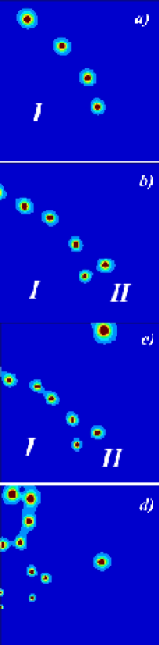
Figure 32: Contour plots of the specific heat in the complex temperature plane for a) $N=11$, b) $N=14$, and c) $N=16$ particles. Panel d) shows the $N=14$ case with weak pairing. The spots indicate the locations of the zeros of the canonical partition function.

In Fig. 32 we show contour plots of the specific heat $\mid C_{v}({\cal B})\mid$ in the complex temperature plane for $N=11$ (a), $14$ (b), and $16$ (c) particles at normal pairing $d/G=0.5$ and the $N=14$ (d) in the strong pairing limit, $d/G=1.5$. The poles are at the center of the dark contour regions. We see evidence of two phases in these systems. The first phase, labeled $I$ in Fig. 32, is a mixed seniority phase, while the second phase, $II$, is a paired phase with zero seniority and exists only in even-$N$ systems. No paired phase exists in the $N=11$ system, and no clear boundaries are evident in the strong pairing case. We find that for (b) and (c) the DOZ are apparently distributed along two lines where the intersection occurs at $\tau_{1}$, which is the point closest to the real axis. As the pairing branch (for $\beta>\beta_{1}$) only encompasses two points, we are unable to precisely determine $\alpha$ along this branch while $\gamma>0$. Based on our free energy results discussed above, we believe $\alpha$ along this branch will be positive. In the mixed phase branch (for $\beta<\beta_{1}$) we find $\gamma<0$, and $\alpha<0$ in all normal-pairing cases.

V.4 Level densities from shell-model Monte Carlo calculations

We also applied shell-model Monte Carlo (SMMC) techniques to survey rare-earth nuclei in the Dy region White et al. (2000). The goal of this extensive study was to examine how the phenomenologically motivated “pairing-plus-quadrupole” interaction compares in exact shell-model solutions with other methods. We also examined how the shell-model solutions compare with experimental data.

We discuss here one particular aspect of that work, namely level density calculations. Details may be found in White et al. (2000). We used the Kumar-Baranger Hamiltonian with parameters appropriate for this region. Our single-particle space included the 50-82 subshell for the protons and the 82-126 shell for the neutrons. While several interesting aspects of these systems were studied in SMMC, we limit our discussion here to the level densities obtained for ¹⁶²Dy.

SMMC is an excellent way to calculate level densities. $E(\beta)$ is calculated for many values of $\beta$ which determine the partition function, $Z$, as

$$\ln[Z(\beta)/Z(0)]=-\int_{0}^{\beta}d\beta^{\prime}E(\beta^{\prime})\;.$$ (104)

$Z(0)$ is the total number of available states in the space. The level density is then computed as an inverse Laplace transform of $Z$. Here, the last step is performed with a saddle point approximation with $\beta^{-2}C\equiv-dE/d\beta$:

$$S(E) = \beta E+\ln Z(\beta)\;,$$ (105)

$$\rho(E) = (2\pi\beta^{-2}C)^{-1/2}\exp(S)\;.$$ (106)

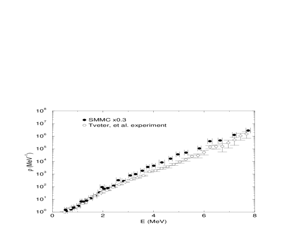
Figure 33: SMMC density vs. experimental data in ¹⁶²Dy.

The comparison of SMMC density in ¹⁶²Dy with the Tveter et al. Tveter et al. (1996) data is displayed in Fig. 33. The experimental method can reveal fine structure, but does not determine the absolute density magnitude. The SMMC calculation is scaled by a factor to facilitate comparison. In this case, the factor has been chosen to make the curves agree at lower excitation energies. From 1-3 MeV, the agreement is very good. From 3-5 MeV, the SMMC density increases more rapidly than the data. This deviation from the data cannot be accounted for by statistical errors in either the calculation or measurement. Near 6 MeV, the measured density briefly flattens before increasing and this also appears in the calculation, but the measurement errors are larger at that point.

The measured density includes all states from the theoretical calculation plus some others, so that one would expect the measured density to be greater than or equal to the calculated density and never smaller. We may have instead chosen our constant to match the densities for moderate excitations and let the measured density be higher than the SMMC density for lower energies (1-3 MeV). Comparing structure between SMMC and data is difficult for the lowest energies due to statistical errors in the calculation and comparison at the upper range of the SMMC calculation, i.e., $E\approx 15$ MeV is unfortunately impossible since the data only extend to about $8$ MeV excitation energy.

VI CONCLUSIONS AND OUTLOOK

Pairing is an essential feature of nuclear systems, with several interesting and unsettled theoretical and experimental consequences, such as superfluidity and neutrino emission in neutron stars or pairing transitions in finite nuclei.

This review is by no means an exhaustive overview; rather, our focus has been on the link between the nuclear many-body problem, and the underlying features of the nuclear force, and selected experimental interpretations and manifestations of pairing in nuclear systems. Our preferred many-body tools have been the nuclear shell model with its effective interactions and various many-body approaches to infinite matter. The common starting point for all these many-body approaches is, however, the free nucleon-nucleon interaction.

Within this setting, we have tried to present and expose several features of pairing correlations in nuclear systems. In particular, we have shown that in neutron star matter (Sec. II), pairing and superfluidity is synonymous with singlet ${}^{1}S_{0}$ and triplet ${}^{3}P_{2}$ pairing up to densities 2-3 times nuclear matter saturation density. For singlet pairing it is the central part of the nucleon-nucleon force which matters, which within a meson-exchange picture can be described in terms of multi-pion exchanges. For triplet pairing, it is the two-body spin-orbit force which provides the attraction necessary for creating a positive pairing gap. Hyperon pairing, especially $\Sigma^{-}$ pairing, is also very likely. However, the actual size of these nucleon and/or hyperon pairing gaps in infinite neutron star matter is an unsettled problem and awaits further theoretical studies. A proper treatment of both short-range and long-range correlations is central to this problem. It will have significant consequences on the emissivity of neutrinos in a neutron star. Color superconductivity in the interior of such compact objects is also an entirely open topic. A similarly unsettled issue is the size of the triplet ${}^{3}S_{1}$ gap in symmetric matter or asymmetric nuclear matter.

The above partial waves are also important for our understanding of pairing properties in finite nuclei. In Sec. III we showed, for example, that the near-constancy of the excitation energy between the ground state with $J=0$ and the first excited state with $J=2$ for the tin isotopes from ¹⁰²Sn to ¹³⁰Sn is essentially due to the same partial waves which yield a finite pairing gap in neutron star matter. Moreover, a seniority analysis of the pairing content of the wave functions for these states shows that we can very well approximate the ground state with a seniority ${\cal S}=0$ state (no broken pairs) and the first excited state in terms of a seniority ${\cal S}=2$ state (one broken pair).

Furthermore, we have used results from large-scale shell-model Monte Carlo and diagonalization calculations to extract information about isoscalar and isovector pairing and thermal response for $fp$-shell nuclei. One key result here was the decrease of $T=1$ pairing correlations as a function of increasing temperature (up to about 1 MeV) and a commensurate buildup of structure in the specific heat curves at the same temperature. Information about proton-neutron pairing and the Wigner energy has also been presented in Sec. III. The important result here was that all $J$ channels of the interaction contribute to the Wigner energy, and that the $J=1$ and $J=J_{\rm max}$ channels contributed most (see also Poves and Martinez-Pinedo (1998)). Proton-neutron pairing is, however, a much more elusive aspect of the nuclear pairing problem. Its actual size, as is also the case in infinite matter, needs further analysis. Our results from Sec. IV may indicate that the $T=0$ part of the pairing interaction does not play a crucial role. For more information, see Zelevinsky et al. (1996); Volya et al. (2002).

Finally, we have tried to analyze recent experimental data on nuclear level densities in terms of pairing correlations. This was done in Sec. V. These data reveal structures in the level density of rare-earth nuclei that can be interpreted as a gradual breaking of pairs. The experimental level densities can also be used to compute the thermal properties such as the entropy or the specific heat. The even systems exhibit a clear bump in the heat capacity. The temperature where this bump appears can be interpreted as a critical temperature for the quenching of pairing correlations. Similar features were also noted in Sec. III (see especially Figs. 20 and 21). More information was also obtained by studying the experimental entropy for even and odd nuclei with those extracted from a simple pairing model with a given number of particles and number of doubly-degenerate particle levels. We showed in Sec. V that the entropy of the odd and even system merge at a temperature which corresponds to the observed bumps in the heat capacity. This temperature occurs typically where we have 2-3 broken pairs.

Within the framework of this simple pairing model, we showed also that for a finite system there is no sudden and abrupt transition to another phase, as we have in an infinite system. Rather, there is a gradual breaking of pairs as temperature increases. However, studying systems with different numbers of particles and levels, we presented also two possible methods for classifying the order of the transition. In order to perform these studies, we needed all eigenvalues from the simple pairing model in order to compute thermodynamical properties. Albeit there have been several interesting theoretical developments of the solution of the model Hamiltonian of Eq. (34) or related models, see for example Richardson (2002); Roman et al. (2002); Volya et al. (2001); Volya (2002), we would like to stress that the investigation of thermodynamic properties requires a knowledge of all eigenvalues.

Furthermore, an obvious deficiency of this simple model in nuclear physics is the lack of long-range correlations, which could, e.g., be expressed via quadrupole terms. A pairing-plus-quadrupole model, as discussed in Sec. III, would however, spoil the simple block-diagonalization feature in terms of seniority as a good quantum number. Such a model is however necessary, since the nuclear force is particular in the sense that the ranges of its short-range and long-range parts are rather similar. This means that short-range contributions arising from e.g., strongly paired particle-particle terms and long-range terms from particle-hole excitations are central for a correct many-body description of nuclear systems, from nuclear matter to finite nuclei. The difficulty connected with these aspects of the nuclear force means that further analysis of the thermodynamics of e.g., rare-earth nuclei can presently only be done in terms of large-scale shell-model Monte Carlo methods.

It should be fairly obvious that we have only been able to cover a very limited aspect of pairing in nuclear systems. We have limited the attention to stable systems. However, pairing correlations are expected to play a special role in drip-line nuclei Dobaczewski et al. (1996). There is currently a considerable experimental effort in nuclear physics, especially due to the advances from radioactive-beam and heavy-ion facilities, which have stimulated an exploration of nuclei far from stability. Many of these nuclei are weakly bound systems. Hence, due to strong surface effects, the properties of such nuclei are perfect laboratories for studies of the density dependence of pairing interactions. An experimental observable that may probe pairing correlations is the pair transfer factor, which is directly related to the pairing density (see Dobaczweski and Nazarewicz (1998) for more details). The difference in the asymptotic behavior of the single-particle density and the pair density in a weakly bound system can be probed by comparing the energy dependence of one-particle and two-particle transfer cross sections. Such measurements, when performed on both stable and neutron rich nuclei, can hopefully shed some light on the asymptotic behavior of pairing. An interesting system here is the chain of tin isotopes beyond ¹³²Sn. Various mean-field calculations Dobaczewski et al. (1996) indicate that there is a considerable increase in the pair transfer form factors for nuclei between ¹⁵⁰Sn and ¹⁷²Sn Dobaczewski et al. (1996). At the moment of writing, $\beta$-decay properties of nuclei like ¹³⁶Sn have just been studied Shergur et al. (2002).

From a many-body point of view, a correct treatment of these weakly bound systems entails an approach which encompasses a proper description of bound states and eventually features from the continuum. Such calculations have recently been mounted within the framework of mean-field and Hartree-Fock-Bogoliubov (HFB) models (see Grasso et al. (2001, 2002)). A finite-range pairing interaction was included explicitely in the calculations. We mention here that the pairing terms in such mean-field calculations can be parameterized from microscopic many-body calculations, as demonstrated by Smerzi et al. Smerzi et al. (1997). However, to include the continuum in a many-body description such as the shell-model with an appropriate effective interaction is highly non-trivial. Even the determination of the effective two-body interaction is an open problem. The low-density studies of singlet ${}^{1}S_{0}$ pairing in dilute Fermi systems Heiselberg et al. (2000) clearly demonstrate that polarization terms cannot be neglected.

We conclude by pointing to the strong similarities between pairing in the nuclear many-body problem and pairing in systems of trapped fermions (see Heiselberg and Mottelson (2002); Bruun and Mottelson (2001) for recent examples). There are also very strong couplings to the experimental and theoretical developments of our understanding of ultra-small superconducting grains Ralph et al. (1995); Black et al. (1996, 1997); von Delft and Ralph (2001); Balian et al. (1999); Mastellone and Falci (1998); Dukelsky and Sierra (1999).

Table 1: $2^{+}_{1}-0^{+}_{1}$ excitation energy for the even tin isotopes ^130-116Sn for various approaches to the effective interaction. See text for further details. Energies are given in MeV.

	116Sn	118Sn	120Sn	122Sn	124Sn	126Sn	128Sn	130Sn
Expt	1.29	1.23	1.17	1.14	1.13	1.14	1.17	1.23
$V_{\mathrm{eff}}$	1.17	1.15	1.14	1.15	1.14	1.21	1.28	1.46
$G$-matrix	1.14	1.12	1.07	0.99	0.99	0.98	0.98	0.97
${}^{1}S_{0}$ $G$-matrix	1.38	1.36	1.34	1.30	1.25	1.21	1.19	1.18
No ${}^{1}S_{0}$ & ${}^{3}P_{2}$ in $G$					0.15	-0.32	0.02	-0.21

Table 2: Seniority $v=0$ overlap (first row) $|\langle^{A}Sn;0^{+}|(S^{\dagger})^{\frac{n}{2}}|\tilde{0}\rangle|^{2}$ and the seniority $v=2$ overlaps (remaining rows) $|\langle^{A}Sn;J_{f}|D^{\dagger}_{JM}(S^{\dagger})^{\frac{n}{2}-1}|\tilde{0}\rangle|^{2}$ for the lowest–lying eigenstates of ^128-120Sn.

	A=128	A=126	A=124	A=122	A=120
$0^{+}_{1}$	0.96	0.92	0.87	0.83	0.79
$2^{+}_{1}$	0.92	0.89	0.84	0.79	0.74
$4^{+}_{1}$	0.73	0.66	0.44	0.13	0.00
$4^{+}_{2}$	0.13	0.18	0.39	0.66	0.74
$6^{+}_{1}$	0.81	0.85	0.83	0.79	0.64

Table 3: $\Delta F/N$ for $T=0.85$ MeV. See text for further details.

$N$	10	12	14	16
$\Delta F/N$ [MeV]	0.531	0.505	0.501	0.495

\begin{picture}(100.0,60.0)\put(0.0,0.0){\epsfbox{dean_hjorthjensen_fig01.ps}} \end{picture}

Figure 1: Possible structure of a neutron star.

\begin{picture}(140.0,140.0)\put(-20.0,-50.0){\epsfbox{dean_hjorthjensen_fig02.ps}} \end{picture}

Figure 2: Plot of the NN interaction for the ${}^{1}S_{0}$ channel employing the Argonne $V_{18}$ interaction Wiringa et al. (1995).

\begin{picture}(140.0,140.0)\put(-20.0,-50.0){\epsfbox{dean_hjorthjensen_fig03.ps}} \end{picture}

Figure 3: Phase shifts for $J\leq 2$ partial waves as function of the incoming energy of two $T=1$ nucleons in the lab system.

\begin{picture}(140.0,140.0)\put(-20.0,-50.0){\epsfbox{dean_hjorthjensen_fig05.ps}} \end{picture}

Figure 5: Plot of the Argonne $V_{18}$ Wiringa et al. (1995) ${}^{3}P_{2}$ partial wave contribution with and without the spin-orbit contribution.

\begin{picture}(140.0,140.0)\put(-20.0,-50.0){\epsfbox{dean_hjorthjensen_fig06.ps}} \end{picture}

Figure 6: ${}^{1}S_{0}$ energy gap in neutron matter with the CD-Bonn, Nijmegen I and Nijmegen II potentials. In addition, we show the results obtained from phase shifts only, Eqs. (43)-(45), and the effective range approximation of Eq. (47). Taken from Elgarøy and Hjorth-Jensen (1998).

Figure 7: Top panel: The angle-averaged ${}^{3}P_{2}$-${}^{3}F_{2}$ gap in neutron matter depending on the Fermi momentum, evaluated with free single-particle spectrum and different nucleon-nucleon potentials. Middle panel: The gap evaluated with BHF spectra. Bottom panel: The gap with the CD-Bonn potential in different approximation schemes. Taken from Baldo et al. (1998b).

\begin{picture}(140.0,140.0)\put(-20.0,-50.0){\epsfbox{dean_hjorthjensen_fig08.ps}} \end{picture}

Figure 8: Effective masses derived from various interactions in the BHF approach. Taken from Baldo et al. (1998b).

Figure 9: Upper box: Proton pairing in $\beta$-stable matter for the ${}^{1}S_{0}$ partial wave. Lower box: Neutron pairing in $\beta$-stable matter for the ${}^{3}P_{2}$ partial wave. Taken from Elgarøy et al. (1996b).

\begin{picture}(140.0,140.0)\put(-20.0,-50.0){\epsfbox{dean_hjorthjensen_fig10.ps}} \end{picture}

Figure 10: EOS for symmetric nuclear matter with the NN potentials and many-body methods described in the text. Taken from Elgarøy et al. (1998).

\begin{picture}(140.0,140.0)\put(-20.0,-50.0){\epsfbox{dean_hjorthjensen_fig11.ps}} \end{picture}

Figure 11: ${}^{3}S_{1}$-${}^{3}D_{1}$ energy gap in nuclear matter, calculated in non-relativistic (full lines) and relativistic (dashed line) approaches. Taken from Elgarøy et al. (1998).

Figure 12: Energy gap in different approximations for the self-energy. The upper line (dashes with crosses) stands for the free single-particle spectrum with a standard BCS approach while the upper solid line arises from the BHF approach of Eq. (49) and the standard BCS approach. The lower lines arise from solving Eq. (9) for the pairing gap with different approaches to the self-energy, for further details see Lombardo et al. (2001b); Lombardo and Schulze (2001). Taken from Lombardo et al. (2001b); Lombardo and Schulze (2001).

\begin{picture}(100.0,60.0)\put(-10.0,-50.0){\epsfbox{dean_hjorthjensen_fig13.ps}} \end{picture}

Figure 13: Diagram (a) is the second-order diagram with particle-hole intermediate states. The external legs can be particles or holes. Diagrams (b) and (c) are examples of third-order TDA or RPA diagrams. The dotted lines represent the interaction vertex.

.

Figure 15: SMMC expectation values of proton and neutron BCS-like pairs after subtraction of the Fermi gas value. Taken from Langanke et al. (1995).

Figure 16: Proton and neutron occupation numbers for various chains of isotopes. Taken from Langanke et al. (1995).

Figure 17: Content of isovector $0^{+}$ pairs and isoscalar $1^{+}$ pairs in the ground states of the isotopes ^54-58Fe. The upper panel shows the diagonal matrix elements of the pair matrix $M_{\alpha\alpha}$. The index $\alpha=1,..,4$ refers to $0^{+}$ pairs in the $f_{7/2}$, $p_{3/2}$, $f_{5/2}$, and $p_{1/2}$ orbitals, respectively. For the isoscalar pairs $\alpha=1,2,3$ refers to $(f_{7/2})^{2}$, $(f_{7/2}f_{5/2})$, and $(f_{5/2})^{2}$ pairs, respectively. The middle panel gives the eigenvalues of the pair matrix; for the isoscalar pairs, only the 3 largest are shown. The lower panel gives the eigenvalues of the pair matrix for the uncorrelated Fermi gas case using Eq. (75). Taken from Langanke et al. (1996).

Figure 18: Largest eigenvalue for the various isovector $0^{+}$ pairs in the $N=Z$ nuclei in the mass region $A=48-56$. Taken from Langanke et al. (1997a).

Figure 19: Calculated displacement $\varepsilon_{W}$ of the binding energy of ²⁴Mg and ⁴⁸Cr from the average parabolic $(N-Z)^{2}$ behavior along an isobaric chain. Shell-model calculations were performed in the $0\hbar\omega$ configuration space. The results of calculations for the binding energies of even-even nuclei along the $A$=48 chain (normalized to ⁴⁸Cr) are shown in the insert. The values of $\varepsilon_{W}$ were obtained using the shell-model Hamiltonian with the $J=1,2,..,J_{\rm max},T=0$ matrix elements removed. For instance, the result for $J_{\rm max}$=3 corresponds to the variant of calculations in which all the two-body matrix elements between states $|j_{1}j_{2}JT$=$0\rangle$ with $J$=1,2,3, were put to zero. The results are normalized to the full shell-model value $\varepsilon_{W}^{\rm total}$ ($J_{\rm max}$=0). The Coulomb contribution to the binding energy has been disregarded. Taken from Satula et al. (1997).

Figure 20: Temperature dependence of various observables in ⁵⁴Fe. Monte Carlo points with statistical errors are shown at each temperature $T$. In the left-hand column, the internal energy, $U$, is calculated as $\langle{\hat{H}}\rangle-E_{0}$, where ${\hat{H}}$ is the many-body Hamiltonian and $E_{0}$ the ground state energy. The heat capacity $C$ is calculated by a finite-difference approximation to $dU/dT$, after $U(T)$ has been subjected to a three-point smoothing, and the level density parameter is $a\equiv C/2T$. In the right-hand column, we show the expectation values of the squares of the proton and neutron BCS pairing fields. For comparison, the pairing fields calculated in an uncorrelated Fermi gas are shown by the solid curve. The moment of inertia is obtained from the expectation values of the square of the total angular momentum by $I=\beta\langle{\hat{J}}^{2}\rangle/3$. Taken from Dean et al. (1994).

Figure 21: The heat capacity of even-even (left panel) and odd-even (right panel) iron isotopes. Taken from Liu and Alhassid (2001).

Figure 22: Temperature dependence of various observables in ⁵⁰Mn. The left panels show (from top to bottom) the total energy, the moment of inertia, and the proton-neutron BCS pairing fields, while the right panels exhibit the expectation values of the isospin operator $\langle\hat{T}^{2}\rangle$, the isovector $J=0$ proton-proton BCS pairing fields, and the isoscalar $J=1$ pairing strength, as defined in the text. For comparison, the solid lines indicate the Fermi gas values of the BCS pairing fields and $J=1$ pairing strength.

Figure 23: Pair correlations, as defined in Eq. 80, for isovector $0^{+}$ and isoscalar $1^{+}$ pairs for ^54-58Fe and ⁵⁶Cr, as functions of temperature. Taken from Langanke et al. (1996).

Figure 24: The distribution of ground state spins in the various random ensembles.

Figure 25: Distribution of the pair transfer coefficient $<\!\!P^{+}_{00}\!\!>$, pairing strength $<\!\!\kappa\!\!>$, and deformation $Q_{2}$ for the random interactions leading to a $J^{\pi}=0^{+}$ ground state in the shell-model description. From left to right we report the results for $N-Z=4$, 2, and 0. The arrows indicate the number of results in a bin when it is out of scale.

Figure 26: Observed entropy for ^161,162Dy as function of excitation energy $E$. Taken from Guttormsen et al. (2000).

Figure 27: Observed entropy for ^171,172Yb as function of excitation energy $E$. Taken from Guttormsen et al. (2000).

Figure 28: Semi-experimental entropy $S$ for ^161,162Dy and ^171,172Yb calculated in the canonical ensemble as a function of temperature $k_{B}T$. Taken from Guttormsen et al. (2000).

Figure 29: Semi-experimental heat capacity as a function of temperature (left panels) and energy $\langle E\rangle$ (right panels) in the canonical ensemble for ^161,162Dy and ^171,172Yb. The dashed lines describe the approximate Fermi gas heat capacity. The arrows indicate the first local maxima of the experimental curve relative to the Fermi gas estimates. The dashed-dotted lines describe extrapolated estimates of the critical temperature $T_{c}$. $T_{c}$ is indicated by the vertical lines. Taken from Schiller et al. (2001).

Figure 30: Entropy in the canonical ensemble as a function of temperature $k_{B}T$ for odd and even systems for $\delta=0.1$ (upper panel), $\delta=0.5$ (central panel), and $\delta=10$ (lower panel). If we wish to make contact with experiment, one can assign units of MeV to $k_{B}T$. The entropy $S/k_{B}$ is dimensionless. Taken from Guttormsen et al. (2000).

Figure 31: Free energy from Eq. (96) at $T=0.5$, $0.85$ and $T=1.0$ MeV with $d/G=0.5$ with 16 particles in 16 doubly degenerate levels. All energies are in units of MeV and an energy bin of $10^{-3}$ MeV has been chosen.

References

- Agrawal et al. (2000) Agrawal, B. K., S. Tapas, J. N. De, and S. K. Samaddar, 2000, Phys. Rev. C 62, 044307.
- Agrawal et al. (2001) Agrawal, B. K., S. Tapas, J. N. De, and S. K. Samaddar, 2001, Phys. Rev. C 63, 024002.
- Ainsworth et al. (1989) Ainsworth, T. L., J. Wambach, and D. Pines, 1989, Phys. Lett. B 222, 173.
- Ainsworth et al. (1993) Ainsworth, T. L., J. Wambach, and D. Pines, 1993, Nucl. Phys. A 555, 128.
- Akmal et al. (1998) Akmal, A., V. R. Pandharipande, and D. G. Ravenhall, 1998, Phys. Rev. C 58, 1804.
- Alford et al. (1999) Alford, A., K. Rajagopal, and F. Wilczek, 1999, Nucl. Phys. B 558, 219.
- Alhassid (1991) Alhassid, Y., 1991, New Trends in Nuclear Collective Dynamics, edited by Y. Abe (Springer).
- Alhassid et al. (1996) Alhassid, Y., G. Bertsch, D. Dean, and S. Koonin, 1996, Phys. Rev. Lett. 77, 1444.
- Alhassid et al. (1999) Alhassid, Y., S. Liu, and H. Nakada, 1999, Phys. Rev. Lett. 83, 4265.
- Alm et al. (1990) Alm, T., G. Röpke, and M. Schmidt, 1990, Z. Phys. A 337, 355.
- Alpar et al. (1995) Alpar, A., U. Kiziloglŭ, and J. van Paradijs, 1995, Lives of the neutron stars (Kluwer).
- Amundsen and Østgaard (1985) Amundsen, L., and E. Østgaard, 1985, Nucl. Phys. A 437, 487.
- Anataraman and Schiffer (1971) Anataraman, N., and J. Schiffer, 1971, Phys. Lett. B 37, 229.
- Arndt et al. (1997) Arndt, R. A., C. H. Oh, I. I. Strakovsky, R. L. Workman, and F. Dohrmann, 1997, Phys. Rev. C 56, 3005.
- Axel (1962) Axel, P., 1962, Phys. Rev. 126, 671.
- Babu and Brown (1973) Babu, S., and G. E. Brown, 1973, Ann. Phys. (N.Y.) 78, 1.
- Bäckmann et al. (1985) Bäckmann, S.-O., G. E. Brown, and J. A. Niskanen, 1985, Phys. Rep. 124, 1.
- Balberg and Barnea (1997) Balberg, S., and N. Barnea, 1997, Phys. Rev. C 57, 409.
- Baldo et al. (1998a) Baldo, M., F. Burgio, and H.-J. Schulze, 1998a, Phys. Rev. C 58, 3688.
- Baldo et al. (2000) Baldo, M., F. Burgio, and H.-J. Schulze, 2000, Phys. Rev. C 61, 055801.
- Baldo et al. (1990) Baldo, M., J. Cugnon, A. Lejeune, and U. Lombardo, 1990, Nucl. Phys. A 515, 409.
- Baldo et al. (1992) Baldo, M., J. Cugnon, A. Lejeune, and U. Lombardo, 1992, Nucl. Phys. A 536, 349.
- Baldo et al. (1998b) Baldo, M., Ø. Elgarøy, L. Engvik, M. Hjorth-Jensen, and H.-J. Schulze, 1998b, Phys. Rev. C 58, 1921.
- Baldo et al. (1995) Baldo, M., U. Lombardo, and P. Schuck, 1995, Phys. Rev. C 52, 975.
- Balian et al. (1999) Balian, R., H. Flocard, and M. Veneroni, 1999, Phys. Rep. 317, 251.
- Barranco et al. (1997) Barranco, F., R. A. Broglia, H. Esbensen, and E. Vigezzi, 1997, Phys. Lett. B 390, 13.
- Barranco et al. (1999) Barranco, F., R. A. Broglia, G. Gori, E. Vigezzi, P. F. Bortignon, and J. Terasaki, 1999, Phys. Rev. Lett. 83.
- Belyaev (1959) Belyaev, S., 1959, Mat. Fys. Medd. Dan. Vid. Selsk. 31, 641.
- Bennaceur et al. (submitted, 2002) Bennaceur, K., D. Dean, B. Barmore, W. Nazarewicz, and C. Özen, submitted, 2002, Phys. Rev. C .
- Bes and Sorensen (1969) Bes, D. R., and A. R. Sorensen, 1969, Adv. Nucl. Phys. 2.
- Bethe (1936) Bethe, H., 1936, Phys. Rev. 50, 332.
- Bijker and Frank (2000) Bijker, R., and A. Frank, 2000, Phys. Rev. Lett. 84, 420.
- Bijker et al. (1999) Bijker, R., A. Frank, and S. Pittel, 1999, Phys. Rev. C 60, 021302.
- Bishop (1991) Bishop, R. F., 1991, Theor. Chim. Acta 80, 95.
- Black et al. (1996) Black, C. T., D. C. Ralph, and M. Tinkham, 1996, Phys. Rev. Lett 76, 688.
- Black et al. (1997) Black, C. T., D. C. Ralph, and M. Tinkham, 1997, Phys. Rev. Lett 78, 4087.
- Bogolyubov (1959) Bogolyubov, N., 1959, Dolk. Akad. Nauk SSSR 119, 244.
- Bohr et al. (1958) Bohr, A., B. Mottelson, and D. Pines, 1958, Phys. Rev. 110, 936.
- Borrmann et al. (2000) Borrmann, P., O. Mulken, and J. Harting, 2000, Phys. Rev. Lett. 84, 3511.
- Bozek (1999) Bozek, P., 1999, Nucl. Phys. A 657, 187.
- Bozek (2000) Bozek, P., 2000, Phys. Rev. C 62, 054316.
- Bozek (2002) Bozek, P., 2002, Phys. Rev. C 65, 034327.
- Brockmann and Machleidt (1990) Brockmann, R., and R. Machleidt, 1990, Phys. Rev. C 42, 1965.
- Broglia et al. (1994) Broglia, R. A., F. V. De Blasio, G. Lazzari, M. C. Lazzari, and P. M. Pizzochero, 1994, Phys. Rev. D 50.
- Brown and Jackson (1976) Brown, G. E., and A. D. Jackson, 1976, The Nucleon-Nucleon Interaction (North-Holland).
- Bruun and Mottelson (2001) Bruun, G. M., and B. Mottelson, 2001, Phys. Rev. Lett. 87, 270403.
- Bulgac (2002) Bulgac, A., 2002, Phys. Rev. C 65, 051305.
- Bulgac and Yu (2002) Bulgac, A., and Y. Yu, 2002, Phys. Rev. Lett. 88, 042504.
- Chadan and Sabatier (1992) Chadan, K., and P. C. Sabatier, 1992, Inverse Problems in Quantum Scattering Theory (Springer).
- Chen et al. (1986) Chen, J. M. C., J. W. Clark, E. Krotschek, and R. A. Smith, 1986, Nucl. Phys. A 451, 509.
- Chen et al. (1983) Chen, J. M. C., R. D. Clark, J. W. Davé, and V. V. Khodel, 1983, Nucl. Phys. A 555, 59.
- Chomaz et al. (2000) Chomaz, P., V. Duflot, and F. Gulminelli, 2000, Phys. Rev. Lett. 85, 3587.
- Civitarese et al. (1989) Civitarese, O., G. Dussel, and A. Zuker, 1989, Phys. Rev. C40, 2900.
- Cooper et al. (1957) Cooper, L., J. Bardeen, and J. Schrieffer, 1957, Phys. Rev. 108, 1175.
- Cooper et al. (1959) Cooper, L. N., R. L. Mills, and A. M. Sessler, 1959, Phys. Rev. 114, 1377.
- D. and Love (1984) D., B., and A. Love, 1984, Phys. Rep. 107, 325.
- D’Agostino et al. (2000) D’Agostino, M., F. Gulminelli, P. Chomaz, M. Bruno, F. Cannata, R. Bougault, F. Gramegna, I. Iori, N. Le Neindre, G. V. Margagliotti, A. Moroni, and G. Vannini, 2000, Phys. Lett. B 473, 219.
- De Blasio et al. (1997) De Blasio, F. V., M. Hjorth-Jensen, Ø. Elgarøy, L. Engvik, G. Lazzari, M. Baldo, and H.-J. Schulze, 1997, Phys Rev. C 56, 2322.
- Dean et al. (1997) Dean, D., S. Koonin, K. Langanke, and P. Radha, 1997, Phys. Lett. B 399, 1.
- Dean et al. (1994) Dean, D., P. Radha, K. Langanke, Y. Alhassid, S. Koonin, and W. Ormand, 1994, Phys. Rev. Lett. 72, 4066.
- Dean et al. (1995) Dean, D. J., S. E. Koonin, K. Langanke, P. B. Radha, and Y. Alhassid, 1995, Phys. Rev. Lett. 74, 2909.
- Decharge et al. (1975) Decharge, J., M. Gerod, and D. Gogny, 1975, Phys. Lett. 55B, 361.
- von Delft and Ralph (2001) von Delft, J., and D. Ralph, 2001, Phys. Rep. 345, 61.
- Demetriou and Goriely (2001) Demetriou, P., and S. Goriely, 2001, Nucl. Phys. A 695.
- Dickhoff et al. (1983) Dickhoff, W. H., A. Faessler, H. Müther, and S. S. Wu, 1983, Nucl. Phys. A 405, 534.
- Dickhoff et al. (1981) Dickhoff, W. H., A. Faessler, J. Meyer-ter Vehn, and H. Müther, 1981, Phys. Rev. C 23, 1154.
- Dickhoff and Müther (1987) Dickhoff, W. H., and H. Müther, 1987, Nucl. Phys. A 473, 394.
- Dinh Dang (1900) Dinh Dang, N., 1900, Z. Phys. A 335, 253.
- D.M.Brink (1955) D.M.Brink, 1955, Ph.D. Thesis, Oxford University .
- Dobaczewski et al. (1996) Dobaczewski, J., W. Nazarewicz, T. Werner, J. Berger, C. Chinn, and J. Decharge, 1996, Phys. Rev. C 53, 2809.
- Dobaczweski and Nazarewicz (1998) Dobaczweski, J., and W. Nazarewicz, 1998, Phil. Trans. R. Soc. Lond. A 356, 2007.
- Døssing et al. (1995) Døssing, T., T. L. Khoo, T. Lauritsen, I. Ahmad, D. Blumenthal, M. P. Carpenter, B. Crowell, D. Gassman, R. G. Henry, R. V. F. Janssens, and D. Nisius, 1995, Phys. Rev. Lett. 75, 1275.
- Duguet et al. (2002a) Duguet, T., P. Bonche, P.-H. Heenen, and J. Meyer, 2002a, Phys. Rev. C 65, 014310.
- Duguet et al. (2002b) Duguet, T., P. Bonche, P.-H. Heenen, and J. Meyer, 2002b, Phys. Rev. C 65, 014311.
- Dukelsky et al. (1991) Dukelsky, J., A. Poves, and J. Retamosa, 1991, Phys. Rev. C 44, 2872.
- Dukelsky and Sierra (1999) Dukelsky, J., and G. Sierra, 1999, Phys. Rev. Lett. 83, 172.
- Egido and Ring (1993) Egido, J., and P. Ring, 1993, J. Phys. G 19, 1.
- Egido et al. (2000) Egido, J. L., L. M. Robledo, and V. Martin, 2000, Phys. Rev. Lett. 85, 26.
- von Egidy et al. (1988) von Egidy, T., H. Schmidt, and A. Behkami, 1988, Nucl. Phys. A 481, 189.
- Elgarøy et al. (1996a) Elgarøy, Ø., L. Engvik, M. Hjorth-Jensen, and E. Osnes, 1996a, Nucl. Phys. A 607, 425.
- Elgarøy et al. (1996b) Elgarøy, Ø., L. Engvik, M. Hjorth-Jensen, and E. Osnes, 1996b, Phys. Rev. Lett. 77, 1428.
- Elgarøy et al. (1996c) Elgarøy, Ø., L. Engvik, M. Hjorth-Jensen, and E. Osnes, 1996c, Nucl. Phys. A 604, 466.
- Elgarøy et al. (1998) Elgarøy, Ø., L. Engvik, M. Hjorth-Jensen, and E. Osnes, 1998, Phys. Rev. C 57, R1069.
- Elgarøy et al. (1996d) Elgarøy, Ø., L. Engvik, E. Osnes, F. V. De Blasio, M. Hjorth-Jensen, and G. Lazzari, 1996d, Phys. Rev. D 54.
- Elgarøy and Hjorth-Jensen (1998) Elgarøy, Ø., and M. Hjorth-Jensen, 1998, Phys. Rev. C 57, 1174.
- Elgarøy and Schulze (2001) Elgarøy, Ø., and H.-J. Schulze, 2001, private communication .
- Elliott (1958) Elliott, J., 1958, Proc. R. Soc. London A 245.
- Emery and Sessler (1960) Emery, V. J., and A. M. Sessler, 1960, Phys. Rev. 119.
- Engel et al. (1996) Engel, J., K. Langanke, and P. Vogel, 1996, Phys. Lett. B 389, 211.
- Engel et al. (1998) Engel, J., K. Langanke, and P. Vogel, 1998, Phys. Lett. B 429, 215.
- Engeland et al. (2002) Engeland, T., M. Hjorth-Jensen, and E. Osnes, 2002, unpublished .
- Erdelyi (1953) Erdelyi, D., 1953, Higher Transcendental Functions, volume I (McGraw-Hill).
- Evans et al. (1981) Evans, J., G. Dussel, E. Maqueda, and R. Perazzo, 1981, Nucl. Phys. A 367, 77.
- Fabrocini et al. (1998) Fabrocini, A., F. Arias de Savedra, G. Có, and P. Folgarait, 1998, Phys. Rev. C 57, 1668.
- Faessler et al. (1976) Faessler, A., K. Sandhya Devi, F. Grummer, K. Schmid, and R. Hilton, 1976, Nucl. Phys. A 256, 106.
- Ferrenberg and Swendsen (1988a) Ferrenberg, A., and R. Swendsen, 1988a, Phys. Rev. Lett. 61, 2635.
- Ferrenberg and Swendsen (1988b) Ferrenberg, A., and R. Swendsen, 1988b, Phys. Rev. Lett. 63, 1195.
- French and Wong (1970) French, J., and S. Wong, 1970, Phys. Lett. B 33, 449.
- Friman and Maxwell (1979) Friman, B., and O. Maxwell, 1979, Ap. J. 232, 541.
- Garrido et al. (2001) Garrido, E., P. Sarriguren, E. Moya de Guerra, U. Lombardo, P. Schuck, and H.-J. Schulze, 2001, Phys. Rev. C 63, 037304.
- Gilbert and Cameron (1965) Gilbert, A., and A. Cameron, 1965, Can. J. Phys. 43, 1446.
- Giovanardi et al. (2002) Giovanardi, N., F. Barranco, R. A. Broglia, and E. Vigezzi, 2002, Phys. Rev. C 65.
- Glendenning (2000) Glendenning, N. K., 2000, Compact Stars (Springer).
- Gold (1969) Gold, T., 1969, Nature 218, 731.
- Goodman (2000) Goodman, A., 2000, Phys. Scr. T 88.
- Goodman (1979) Goodman, A. L., 1979, Adv. Nucl. Phys. 11, 263.
- Goodman (1981a) Goodman, A. L., 1981a, Nucl. Phys. A 352, 30.
- Goodman (1981b) Goodman, A. L., 1981b, Nucl. Phys. A 352, 45.
- Gorkov and Melik-Barkhudarov (1961) Gorkov, L. P., and T. K. Melik-Barkhudarov, 1961, Sov. Phys. JETP 13.
- Grasso et al. (2001) Grasso, M., N. Sandulescu, N. Van Giai, and R. J. Liotta, 2001, Phys. Rev. C 64, 064321.
- Grasso et al. (2002) Grasso, M., N. Van Giai, and N. Sandulescu, 2002, Phys. Lett. B 535, 103.
- Gross (1997) Gross, D., 1997, Phys. Rep. 279, 119.
- Gross and Votyakov (2000) Gross, D., and E. Votyakov, 2000, Eur. Jour. Phys. B 15, 115.
- Grossmann and Lehmann (1969) Grossmann, S., and V. Lehmann, 1969, Z. Phys. 218, 449.
- Grossmann and Rosenhauer (1967) Grossmann, S., and W. Rosenhauer, 1967, Z. Phys. 207, 138.
- Grossmann and Rosenhauer (1969) Grossmann, S., and W. Rosenhauer, 1969, Z. Phys. 218, 439.
- Guimarães et al. (1996) Guimarães, F. B., B. V. Carlson, and T. Frederico, 1996, Phys. Rev. C 54, 2385.
- Guttormsen et al. (2000) Guttormsen, M., A. Bjerve, M. Hjorth-Jensen, E. Melby, J. Rekstad, A. Schiller, S. Siem, and A. Belić, 2000, Phys. Rev. C 62, 024306.
- Hagino and Bertsch (2000) Hagino, K., and G. F. Bertsch, 2000, Nucl. Phys. A 679, 163.
- Hagino et al. (2002) Hagino, K., P.-G. Reinhard, and G. F. Bertsch, 2002, Phys. Rev. C 65.
- Heiselberg and Hjorth-Jensen (2000) Heiselberg, H., and M. Hjorth-Jensen, 2000, Phys. Rep. 328, 237.
- Heiselberg and Mottelson (2002) Heiselberg, H., and B. Mottelson, 2002, Phys. Rev. Lett. 88, 190401.
- Heiselberg et al. (2000) Heiselberg, H., C. J. Pethick, H. Smith, and L. Viverit, 2000, Phys. Rev. Lett. 85, 2418.
- Henden et al. (1995) Henden, L., L. Bergholt, M. Guttormsen, J. Rekstad, and T. Tveter, 1995, Nucl. Phys. A 589, 249.
- Hewish et al. (1968) Hewish, A., J. S. Bell, J. D. H. Pilkington, P. F. Scott, and R. A. Collins, 1968, Nature 217, 709.
- Hilaire et al. (2001) Hilaire, S., J. Delaroche, and M. Girod, 2001, Eur. Phys. J. A 12.
- Hjorth-Jensen (2002) Hjorth-Jensen, M., 2002, Advances in Many-Body Physics, edited by N. Walet and R. F. Bishop, volume 2 (World Scientific).
- Hjorth-Jensen et al. (1995) Hjorth-Jensen, M., T. T. S. Kuo, and E. Osnes, 1995, Phys. Rep. 261, 125.
- Holt et al. (1998) Holt, A., T. Engeland, M. Hjorth-Jensen, and E. Osnes, 1998, Nucl. Phys. A 634, 41.
- Horoi et al. (2001) Horoi, M., B. B.A., and V. Zelevinsky, 2001, Phys. Rev. Lett. 87, 062501.
- Iachello and Arima (1988) Iachello, A., and A. Arima, 1988, The Interacting Boson Model (Cambridge University Press).
- Jackson (1983) Jackson, A. D., 1983, Ann. Rev. Nucl. Part. Sci. 33, 105.
- Jackson et al. (1982a) Jackson, A. D., E. Krotschek, D. E. Meltzer, and R. A. Smith, 1982a, Nucl. Phys. A 386, 125.
- Jackson et al. (1982b) Jackson, A. D., A. Lande, and R. A. Smith, 1982b, Phys. Rep. , 1.
- Jänecke (1965) Jänecke, J., 1965, Nucl. Phys. 73, 97.
- Jenkins et al. (2002) Jenkins, D. G., N. S. Kelsall, C. J. Lister, D. P. Balamuth, M. P. Carpenter, T. A. Sienko, S. M. Fischer, R. M. Clark, P. Fallon, A. Görgen, A. O. Macchiavelli, C. E. Svensson, et al., 2002, Phys. Rev. C 65.
- Jensen et al. (1984) Jensen, A., P. Hansen, and B. Jonson, 1984, Nucl. Phys. A 431, 393.
- Jeukenne et al. (1976) Jeukenne, J. P., A. Lejeune, and C. Mahaux, 1976, Phys. Rep. 25C, 83.
- Johnson et al. (1971) Johnson, A., H. Ryde, and J. Sztarkier, 1971, Phys. Lett. B 34.
- Johnson et al. (1998) Johnson, C., G. Bertsch, and D. Dean, 1998, Phys. Rev. Lett. 80, 2749.
- Johnson et al. (2000) Johnson, C., G. Bertsch, D. Dean, and I. Talmi, 2000, Phys. Rev. C 61, 14311.
- Kaplan et al. (2001) Kaplan, L., T. Papenbrock, and C. Johnson, 2001, Phys. Rev. C 63, 014307.
- Kerman et al. (1961) Kerman, A., R. Lawson, and M. Macfarlane, 1961, Phys. Rev. 124, 162.
- Kisslinger and Sorensen (1960) Kisslinger, L. S., and R. A. Sorensen, 1960, Mat. Fys. Medd. Dan. Vid. Selsk. 32, no. 9.
- Kodel et al. (1996) Kodel, V. A., V. V. Kodel, and J. W. Clark, 1996, Nucl. Phys. A 598, 390.
- Kodel et al. (1998) Kodel, V. A., V. V. Kodel, and J. W. Clark, 1998, Phys. Rev. Lett. 81, 3828.
- Kodel et al. (2001) Kodel, V. A., V. V. Kodel, and J. W. Clark, 2001, Nucl. Phys. A 679, 827.
- Koonin et al. (1997) Koonin, S., D. Dean, and K. Langanke, 1997, Phys. Rep. 278, 1.
- Krappe et al. (1979) Krappe, H., J. Nix, and A. Sierk, 1979, Phys. Rev. C 20, 992.
- Krotscheck and Clark (1983) Krotscheck, E., and A. D. Clark, J. W.and Jackson, 1983, Phys. Rev. B 28, 5088.
- Krotscheck and Clark (1980) Krotscheck, E., and J. W. Clark, 1980, Nucl. Phys. A 333, 77.
- Krotscheck et al. (1981) Krotscheck, E., R. A. Smith, and A. D. Jackson, 1981, Phys. Rev. B 24, 6404.
- Kucharek and Ring (1991) Kucharek, H., and P. Ring, 1991, Z. Phys. A 339, 23.
- Kucharek et al. (1989) Kucharek, H., P. Ring, P. Schuck, R. Bengtsson, and M. Girod, 1989, Phys. Lett. B 216, 249.
- Kusnezov (2000) Kusnezov, D., 2000, Phys. Rev. Lett. 85, 3773.
- Kusnezov et al. (2000) Kusnezov, K., N. Zamfir, and R. Casten, 2000, Phys. Rev. Lett. 85, 1396.
- Kwong and Köhler (1997) Kwong, N. H., and S. Köhler, 1997, Phys. Rev. C 55, 1650.
- Lacombe et al. (1980) Lacombe, M., B. Loiseau, J. M. Richard, R. Vinh Mau, J. Côte, P. Pirès, and R. de Tourreil, 1980, Phys. Rev. C 21, 861.
- Lamb (1991) Lamb, F. K., 1991, Frontiers of stellar evolution, edited by D. L. Lambert (Astronomy Society of the Pacific).
- Langanke et al. (1997a) Langanke, K., D. Dean, S. Koonin, and P. Radha, 1997a, Nucl. Phys. A 613, 253.
- Langanke et al. (1995) Langanke, K., D. Dean, P. Radha, Y. Alhassid, and S. Koonin, 1995, Phys. Rev. C 52, 718.
- Langanke et al. (1996) Langanke, K., D. Dean, P. Radha, and S. Koonin, 1996, Nucl. Phys. A 602, 718.
- Langanke et al. (1997b) Langanke, K., P. Vogel, and D.-C. Zheng, 1997b, Nucl. Phys. A 626.
- Lauritzen et al. (1993) Lauritzen, B., A. Anselmino, P. F. Bortignon, and R. A. Broglia, 1993, Ann. Phys. (NY) 223, 216.
- Lee and Kosterlitz (1990) Lee, J., and J. Kosterlitz, 1990, Phys. Rev. Lett. 65, 137.
- Lee and Kosterlitz (1991) Lee, J., and J. Kosterlitz, 1991, Phys. Rev. B 43, 3265.
- Lipkin (1960) Lipkin, H., 1960, Ann. of Phys. 31, 525.
- Liu and Alhassid (2001) Liu, S., and Y. Alhassid, 2001, Phys.Rev.Lett. 87, 022501.
- Lombardo et al. (2001a) Lombardo, U., P. Nozieres, P. Schuck, H.-J. Schulze, and A. Sedrakian, 2001a, Phys. Rev. C 64.
- Lombardo and Schuck (2001) Lombardo, U., and P. Schuck, 2001, Phys. Rev. C 63, 038201.
- Lombardo et al. (2001b) Lombardo, U., P. Schuck, and W. Zuo, 2001b, Phys. Rev. C 64, 021301.
- Lombardo and Schulze (2001) Lombardo, U., and H.-J. Schulze, 2001, Lect. Notes Phys., volume 578 (Springer).
- M. Schmidt et al. (2001) M. Schmidt, M., R. Kusche, T. Hippler, J. Donges, W. Kronmüller, B. von Issendorff, and H. Haberland, 2001, Phys. Rev. Lett 86, 1191.
- Ma. et al. (2000) Ma., W. C., V. Martin, T. L. Khoo, T. Lauritsen, J. L. Egido, I. Ahmad, P. Bhattacharyya, M. P. Carpenter, J. P. Daly, Z. W. Grabowksy, J. H. Hamilton, R. V. F. Janssens, et al., 2000, Phys. Rev. Lett. 84, 5967.
- Machleidt (1989) Machleidt, R., 1989, Adv. Nucl. Phys. 19, 189.
- Machleidt (2001) Machleidt, R., 2001, Phys. Rev. C 63, 024001.
- Machleidt et al. (1996) Machleidt, R., F. Sammarruca, and Y. Song, 1996, Phys. Rev. C 53, 1483.
- Mastellone and Falci (1998) Mastellone, A., and R. Falci, G. Fazio, 1998, Phys. Rev. Lett. 80, 4542.
- Matera et al. (1997) Matera, F., G. Fabbri, and A. Dellafiore, 1997, Phys. Rev. C 56, 228.
- Mayer (1950) Mayer, M., 1950, Phys. Rev. 78, 22.
- Melby et al. (1999) Melby, E., L. Bergholt, M. Guttormsen, M. Hjorth-Jensen, F. Ingebretsen, S. Messelt, J. Rekstad, A. Schiller, S. Siem, and S. Ødegard, 1999, Phys. Rev. Lett. 83, 3150.
- Melby et al. (2001) Melby, E., M. Guttormsen, J. Rekstad, A. Schiller, S. Siem, , and A. Voinov, 2001, Phys. Rev. C 63, 044309.
- Migdal (1959) Migdal, A., 1959, Nucl. Phys. 13, 655.
- Migdal (1960) Migdal, A., 1960, Sov. Phys. JETP 10, 176.
- Molinari et al. (1975) Molinari, A., M. Johnson, A. Bethe, and W. Alberico, 1975, Nucl. Phys. A 239, 45.
- Moretto et al. (2001) Moretto, L. G., J. B. Elliott, L. Phair, and G. J. Wozniak, 2001, preprint nucl-th/0012037 .
- Mottelson and Valantin (1960) Mottelson, B., and J. Valantin, 1960, Phys. Rev. Lett. 5, 511.
- Mueller and Sherril (1993) Mueller, A. C., and B. M. Sherril, 1993, Ann. Rev. Nucl. Part. Phys. 43, 529.
- Muhlhans et al. (1983) Muhlhans, K., E. Muller, U. Mosel, and A. Goodman, 1983, Z. PHys. A 313, 133.
- Mulhall et al. (2000) Mulhall, D., A. Volya, and V. Zelevinsky, 2000, Phys. Rev. Lett. 85, 4016.
- Müther et al. (1985) Müther, H., A. Polls, and T. T. S. Kuo, 1985, Nucl. Phys. A 435, 548.
- Myers (1977) Myers, W., 1977, Droplet model of atomic nuclei (Plenum).
- Myers and Swiatecki (1966) Myers, W., and W. Swiatecki, 1966, Nucl. Phys. A 81, 1.
- Nakada and Alhassid (1997) Nakada, H., and Y. Alhassid, 1997, Phys. Rev. Lett. 79, 2939.
- Nayak and Pearson (1995) Nayak, R., and J. Pearson, 1995, Phys. Rev. C 52, 2254.
- Newton (1956) Newton, T., 1956, Can. J. Phys. 36, 804.
- Nogami (1964) Nogami, Y., 1964, Phys. Rev. 134, 313.
- Nozieres and Schmitt-Rink (1985) Nozieres, P., and S. Schmitt-Rink, 1985, J. Low Temp. Phys. 59, 195.
- Oganessian et al. (1999) Oganessian, Y. T., V. Zagrebaev, and J. Vaagen, 1999, Phys. Rev. Lett. 82, 4996.
- Page et al. (2000) Page, D., M. Prakash, J. M. Lattimer, and A. Steiner, 2000, Phys. Rev. Lett. 85, 2048.