Basis Generator for M-Scheme SU(3) Shell Model Calculations

Abstract

A FORTRAN code for generating the leading $SU(3)$ irreducible representation (irrep) of $N$ identical spin ${}^{1}/_{2}$ fermions in a harmonic oscillator mean field is introduced. The basis states are labeled by $N$ – the total number of particles, the $SU(3)$ irrep labels ($\lambda,\mu$), and $S$ – the total spin of the system. The orthonormalized basis states have two additional good quantum numbers: $\epsilon$ – the eigenvalue of the quadruple operator, $Q_{0}$; and $M_{J}$ – the eigenvalues of the projection of the total angular momentum operator, $J_{0}=L_{0}+S_{0}$. The approach that is developed can be used for a description of nuclei in a proton-neutron representation and is part of a larger program aimed at integrating $SU(3)$ symmetry into the best of the currently available exact shell-model technologies.

1 Introduction

Successful models for describing energy spectra, transition strengths and other nuclear phenomena usually work well in one region of a shell but not in others. For example, the random phase approximation (RPA) [1] is a reasonable theory for describing properties of nuclei near closed shells but fails in mid-shell regions where deformation is the most characteristic feature due to the importance of the quadruple-quadrupole ($Q\cdot Q$) interaction [2] in this domain. For near mid-shell nuclei, algebraic models based on $SU(3)$ [3] work best since the basis states are then eigenstates of $Q\cdot Q$.

Applications of a nuclear shell-model theory always involve three considerations [4]:

• Step 1: Selection of a model space based on a simplified Hamiltonian. Frequently used approximations include the Simple Harmonic Oscillator Hamiltonian for near closed-shell nuclei and a Nilsson Hamiltonian for deformed systems.

• Step 2: Diagonalization of a realistic Hamiltonian in the model space to obtain the energy spectrum and eigenstates of the system under consideration. Important components of a realistic Hamiltonian include the $Q\cdot Q$ and pairing ($P$) interactions as well as single-particle $l\cdot l$ and $l\cdot s$ terms.

• Step 3: Evaluation of electromagnetic transition strengths (E2, M1, etc.) between calculated eigenstates and a comparison with the available experimental data.

If the model Hamiltonian includes free parameters, for example, single-particle energies and/or the strength of the $Q\cdot Q$ and $P$ interactions, the procedure is repeated to obtain a best overall fit to the experiment data.

The easiest to use of modern shell-model codes are based on the so-called M-scheme logic, namely, model spaces spanned by many-particle configurations (Slater determinants) with good projection of the total angular momentum [5, 6]. Good total angular momentum, which is a conserved symmetry due to the isotropy of space, is obtained by angular momentum projection. Codes of this type normally yield a good description of the single-particle nuclear phenomena; unfortunately, an equally good description of collective phenomena within the framework of such a theory is very difficult to achieve. On other hand, an $SU(3)$ based shell-model scheme is designed to give a simple interpretation of collective phenomena. An ideal scenario would incorporate both, allowing the Hamiltonian of the system to “choose” which one of the two (or an admixture) is most appropriate.

A project, code named Red Stick for Baton Rouge, is now under development at Louisiana State University. Principal authors are Jerry Draayer, Erich Ormand, Calvin Johnson, and Vesselin Gueorguiev. The goal of the project is to develop a new M-scheme shell-model code that allows the user to include $SU(3)$ symmetry-adapted basis states in addition to (the usual) single-particle based configurations.

In this paper we discuss the first stage of the Red Stick project – a basis generator for $M$-scheme $SU(3)$ shell-model configurations. We begin with a review of $SU(3)$ shell-model basics [7, 8]. Then we introduce an appropriate single-particle level scheme and give matrix elements of the generators of $SU(3)$ in that representation. Next we consider the structure of the Highest Weight State (HWS) of an $SU(3)$ irrep, and especially the HWS of so-called leading $SU(3)$ irreps. Once a HWS is known, we then go on to show how all states of that irrep can be constructed using $SU(3)$ step operators [9]. States with good projection of the total angular momentum $M_{J}$ are obtained by considering the direct product $SU(3)\otimes SU_{S}(2)$. Some information about the FORTRAN code that uses these techniques will also be presented.

1.1 $SU(3)$ Basics

In this section we review group theoretical concepts that are important to the development of the theory and introduce $SU(3)$ conventions adopted in our discussion. We also consider the physical reduction $SU(3)\supset SO(3)$ and the canonical reduction $SU(3)\supset U(1)\otimes SU(2)$ with their respective labels.

First consider the so-called physical reduction $SU(3)\supset SO(3)$, which yields a convenient labeling scheme for the generators of $SU(3)$ in terms of $SO(3)$ tensor operators. The commutation relations for these $SU(3)\supset SO(3)$ tensor operators are given in terms of ordinary $SO(3)$ Clebsch-Gordan coefficients (CGC) [7]:

$$[L_{m},L_{m^{\prime}}] = -\sqrt{2}(1m,1m^{\prime}|1m+m^{\prime})L_{m+m^{\prime}}$$

$$[Q_{m},L_{m^{\prime}}] = -\sqrt{6}(2m,1m^{\prime}|2m+m^{\prime})Q_{m+m^{\prime}}$$ (1)

$$[Q_{m},Q_{m^{\prime}}] = 3\sqrt{10}(2m,2m^{\prime}|1m+m^{\prime})L_{m+m^{\prime}}$$

Within this reduction scheme, states of an $SU(3)$ irrep $(\lambda,\mu)$ have the following labels:

• $(\lambda,\mu)$ – $SU(3)$ irrep labels;

• $l$ – total orbital angular momentum, which corresponds to the second order Casimir operator of $SO(3)$;

• $m_{l}$ – projection of the angular momentum along the laboratory $z$-axis;

• $k$ – projection of the angular momentum in a body-fixed frame, which is related to multiple occurrences of $SO(3)$ irreps with angular momentum $l$ in the $(\lambda,\mu)$ irrep.

Unfortunately, this scheme has only one additive label, namely $m_{l}$, and in addition, there are technical difficulties associated with handling the $k$ label.

The labeling scheme for this project is the canonical reduction $SU(3)\supset U(1)\otimes SU(2)$ where $Q_{0}$ is the $U(1)$ generator and the $SU(2)$ generators are proportional to $L_{0}$, $Q_{+2}$, and $Q_{-2}$ [7]. Under the action of the generators of these $U(1)$ and $SU(2)$ groups, the remaining four generators of $SU(3)$ transform as two conjugate spin $[\frac{1}{2}]$ $SU(2)$ tensors with $\varepsilon=\pm 3$ values for $Q_{0}$. For this scheme, states of a given $SU(3)$ irrep $(\lambda,\mu)$ have the following labels:

• $(\lambda,\mu)$ – $SU(3)$ irrep labels,

• $\varepsilon$ – quadruple moment ($Q_{0}$),

• $m_{l}$ – projection of the orbital angular momentum ($L_{0}$),

• $n_{\rho}$ – related to the second order Casimir operator of $SU(2)$, which for symmetric $(\lambda,0)$ irreps is simply the number of oscillator quanta in the $(x,y)$ plane.

This canonical reduction, $SU(3)\supset U(1)\otimes SU(2)$, has two additive labels, $\varepsilon$ ($Q_{0}$) and $m_{l}$ ($L_{0}$) and the allowed values of these labels for fixed $SU(3)$ irrep $(\lambda,\mu)$ are given by [9]:

$$\varepsilon = 2\lambda+\mu-3(p+q)$$ (2)

$$n_{\rho} = \mu+(p-q)$$

$$m_{l} = n_{\rho}-2m$$

where $0\leq p\leq\lambda$ , $0\leq q\leq\mu$ , and $0\leq m\leq n_{\rho}.$

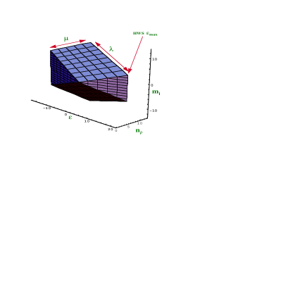
Figure 1: Three-dimensional view of the $(\lambda,\mu)$ $SU(3)$ irrep.

2 Basis State Generation

The algorithm we use to generate $SU(3)$ symmetry adapted states with good projection of the total angular momentum is described in this section. It consists of four basic components: 1) definition of the single-particle levels and matrix elements of the $SU(3)$ generators for a given shell; 2) generation of the HWS of $SU(3)\otimes SU_{S}(2)$ for given number of fermions $N$ and spin $S$; 3) generation of the other $SU(3)$ states by applying step operators to the HWS; and 4) generation of states of good total angular momentum projection, $M_{J}$. This will be followed by a short discussion of a FORTRAN code that uses the algorithm.

2.1 Single-particle Levels – Ordering Scheme

Single-particle levels of the $\eta=0,1,2,...$ $(s,p,sd,...)$ harmonic oscillator shell belong to the symmetric $(\eta,0)$ irrep of $SU(3)$. Because $\mu=0$, a typical three-dimensional representation of $SU(3)$ basis states, Fig.1, reduces to a special two-dimensional triangular shape ($\varepsilon$ and $n_{\rho}$ become linearly dependent), Fig.2. Also, because $SU(3)$ is a compact group its irreps are finite dimensional and many-particle (fermion) configurations can be conveniently represented as binary strings with a $1$ or $0$ representing the presence or absence of a particle in the corresponding single-particle level. (The latter, together with a “sign rule” to accommodate fermion statistics, is a convenient computer native implementation of a Slater determinant representation of the basis states.)

A convenient ordering scheme (which tracks the arrows in Fig.2) is set by requiring a simple representation of many-particle configurations with maximum quadruple deformation. This objective can be achieved if the states are ordered by $\varepsilon$ (quadruple moment) first and then by $m_{l}$ (projection of the total angular momentum).

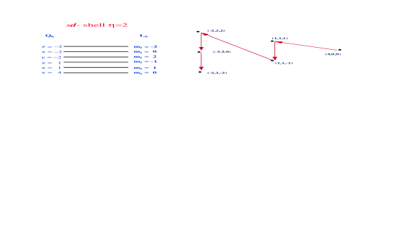
Figure 2: Ordering scheme of the single-particle levels.

2.2 Action of $SU(3)$ Generators on Single-particle States

To be able to apply the $SU(3)$ generators on many-particle configurations it suffices to know the action of these generators on the single-particle states. The eight generators of $SU(3)$ belong to the self-adjoint $(1,1)$ irrep of $SU(3)$. The operator structure should be chosen in the most convenient form for the application under consideration. For the present application, this choice is the same as used for the basis states, namely, the $SU(3)\supset SU(2)\otimes U(1)$ reduction. The matrix elements of the $SU(3)$ generators can be obtained either by using an application of the appropriate Wigner-Eckert theorem or by using explicit expressions [9] for determining the action of the operators on the basis states. For computational purposes it is better to adopt a direct solution, one that exploits the fact that the action is on a product of single-particle levels each of which belongs to a symmetric $(\eta,0)$ irrep of $SU(3)$. This allows the matrix elements of the $SU(3)$ generators to be calculated using properties of the $SU(2)$ only (Fig.3).

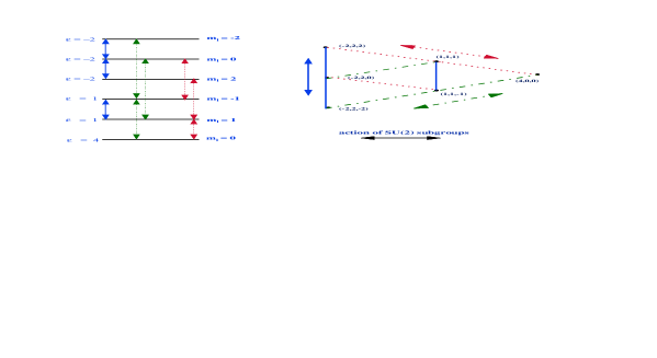
Figure 3: The diagram on the right shows the action of the six non-diagonal generators of $SU(3)$. The vertical solid lines represent the action of the $SU(2)$ subgroup that enters the $SU(3)\supset SU(2)\otimes U(1)$ chain. The diagram on the left shows that applying an $SU(3)$ generator to a single-particle state results in another single-particle state.

A key feature is the fact that the six non-diagonal generators of $SU(3)$ (recall that $L_{0}$ and $Q_{0}$ are diagonal) are rising or lowering generators of $SU(2)$ subgroups of $SU(3)$. The three $SU(2)$ subgroups and their respective actions are shown in Fig. 3. States that are collinear with one of the sides of the triangular shape shown on the right in the figure form an irrep of the corresponding $SU(2)$ subgroup.

2.3 Highest Weight States of $SU(3)\otimes SU_{S}(2)$ for Leading Irreps

So far we have constructed single-particle states and evaluated matrix elements of the generators of $SU(3)$ when they act on these states. The next step is to construct many-particle HWS of $SU(3)\otimes SU_{S}(2)$. In the chosen scheme there are seven extreme states which correspond to the vertexes of the three-dimensional diagram (Fig.1) of a general $(\lambda,\mu)$ irrep. We are particularly interested in the vertex that has the maximum value for the quadruple moment of the system (Fig.1). Our HWS is the state with $\varepsilon=2\lambda+\mu$, $n_{\rho}=\mu$, and $m_{l}=\mu$. This HWS (maximum value of $m_{l}$ for maximum $\varepsilon$) can be easily constructed by ensuring that the action of the $SU(3)$ rising generators annihilate it. Indeed, for such a HWS the values of $\lambda$ and $\mu$ can be determined from its $\varepsilon$ and $m_{l}$ labels.

Selecting the leading $(\lambda,\mu)$ irrep (HWS with maximum overall value of $\varepsilon$) out of all possible irreps of an $N$ fermion system with total system spin $S$ is very simple within the chosen scheme. This is because the number of particles with spin up $n_{\uparrow}$ and spin down $n_{\downarrow}$ is uniquely determined by the solution of two linear equations:

$$N = n_{\uparrow}+n_{\downarrow}$$

$$2S = n_{\uparrow}-n_{\downarrow}.$$

Where the second equation expresses the fact that we also require the state to be highest weight with respect to $SU_{S}(2)$. Further, maximizing the value of $Q_{0}$ is achieved by filling the single-particle states of the $(\eta,0)$ irrep (Fig.2) from bottom to top. The chosen scheme ensures that this simple procedure gives maximum values for $\varepsilon$ and $m_{l}$. The $SU(3)$ irrep labels $(\lambda,\mu)$ are obtained by evaluating the quadruple moment $Q_{0}$ and projection of the angular momentum $L_{0}$, as these are additive quantum numbers.

For example, in the $sd$–shell, there are six single-particle levels corresponding to the $(2,0)$ irrep of $SU(3)$. The HWS of the leading irrep for $N=6$ particles and total system spin $S=1$ is $(3,3)$ (Fig.4), whereas for $S=0$ the leading $SU(3)$ irrep is $(6,0)$ (Fig.5). These many-particle configurations are HWS with respect to $SU(3)$ as well as $SU_{S}(2)$.

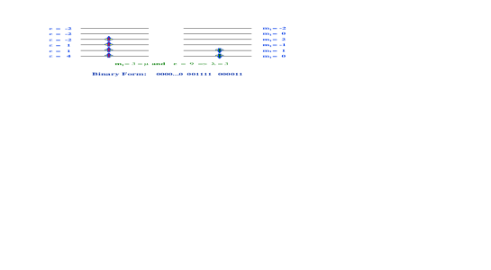
Figure 4: Highest weight state of the leading $(3,3)$ irrep for $N=6$ and $S=1$ in the $sd$–shell.

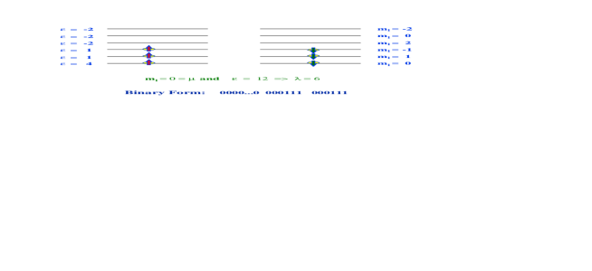
Figure 5: Highest weight state of the leading $(6,0)$ irrep for $N=6$ and $S=0$ in the $sd$–shell.

2.4 Generating $SU(3)$ States with Step Operators

Once we have the HWS of $SU(3)$ $\otimes$ $SU_{S}(2)$, we can generate any other state of the $SU(3)$ irrep $(\lambda,\mu)$ by applying step operators similar to those given by Hecht. By using the parameterization (2) [9], we can identify the corresponding step operators, Fig. 6.

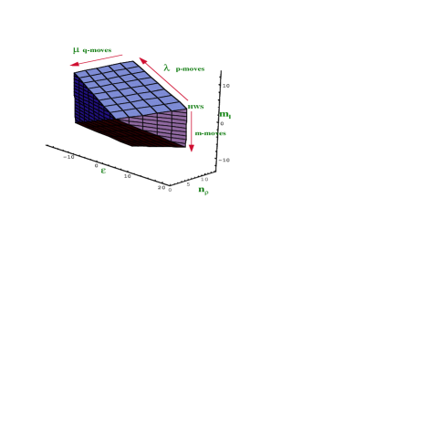
Figure 6: Action of the $SU(3)$ step operators.

It is important to note that applying $p$–move or $q$–move step operators to states on the top surface yields other states (or zero) on that same surface. Since the states on the top surface are HWS with respect to $SU(2)$ in the $SU(3)$ $\supset$ $SU(2)\otimes U(1)$ reduction, the $m$–move step operator is an $SU(2)$ lowering operator which changes the projection of the angular momentum, $m_{l}$. The $p$–move and $q$–move step operators can be obtained by imposing the restriction that they generate only transformations within the $SU(2)$ HWS space. From an algebraic perspective, the $p$–move and the $m$–move operators are linear in $SU(3)$ generators while the $q$–move operator is quadratic. Nevertheless, the state generation process can be written in such a way that the $q$–move operator effectively reduces to a linear action. These step operators can also be obtained by a projection operator technique [10].

2.5 Generating States of Good $M_{J}$ by Lowering the Spin

Since the action of $SU(3)$ commutes with that of the spin, $SU_{S}(2)$, it is not difficult to achieve the final goal of states with good total angular momentum projection, $M_{J}$. Recall that we started with the HWS of $SU(3)$ $\otimes$ $SU_{S}(2)$. We then introduced a procedure to generate other states of the $SU(3)$ irrep by applying step operators. Each of these states remains a HWS of $SU_{S}(2)$. By applying spin lowering operators to $SU(3)$ states with $m_{l}=M_{J}-m_{s}$, we can generate states with labels: $N$, $S$ , $(\lambda,\mu)$, $\varepsilon$, $n_{\rho}$, $m_{l}$, and $M_{J}$.

2.6 About the FORTRAN code

A FORTRAN code that uses the above algorithm was run on three platforms: Macintosh IIci, Power Macintosh 8500, and SUN workstation. Here we give some of the run-time characteristics of the code for shells below the $sdg$–shell:

• On a $50$ MHz Macintosh IIci with math co-processor, $3$ Mb of memory suffices and the longest run time for generating all states of any leading $SU(3)$ irrep was less than $5$ min.

• On a $200$ MHz Power Macintosh $8500$, $4$ Mb of memory was sufficient and the longest run time for generating all states of any leading $SU(3)$ irrep was less than $30$ sec.

• On a $200$ MHz SUN workstation the longest run time for generating all states of any leading $SU(3)$ irrep was less than $15$ sec. All states with good $M_{J}$ for any leading irrep of $SU(3)$ $\otimes$ $SU_{S}(2)$ for the $p,sd,$ and $pf$ shells can be generated in less than $20$ min.

Beyond the $pf$–shell ($\eta\geq 4$), the number of configurations in a single $SU(3)$ state may exceed $100,000$. The storage requirement must be pushed up accordingly. More storage is also needed because beyond the $sdg$–shell the number of single-particle states exceed $16$ ($32$ with the spin degree of freedom) which means more than a single word is required to represent many-particle configurations.

3 Summary and Discussion

An $SU(3)$ basis state generator for producing states with good projection of the total angular momentum, $M_{J}$, and therefore one that is suitable for integration into modern $M$-scheme shell-model codes, is suggested as a possible way to obtain simultaneously a description of collective and single-particle nuclear phenomena. Indeed, a basis state generator that uses the algorithm described above and generates $SU(3)$ states as a sum of Slater determinants (many-particle configurations) with good $M_{J}$ is available. The basis state generation procedure consists of four main components as follows:

• Symmetric irreps of $SU(3)$ are chosen as single-particle shell-model states,

• many-particle state is constructed as HWS of $SU(3)$ $\otimes$ $SU_{S}(2)$,

• $SU(3)$ step operators are applied to obtain other states within an $SU(3)$ irrep,

• and finally, states with good $M_{J}$ are then obtained by $SU_{S}(2)$ lowering operators.

There are additional things that need to be done, especially the generation of other then leading irreps of $SU(3)$. This can be achieved by employing an algorithm for generating non-leading HWS that is part of an $SU(3)$ reduced matrix element package [11] or perhaps by using another more direct approach tailored to the present application. The generation of other HWS is important if one wishes to include states that are not maximally deformed in their intrinsic configuration in a calculation. For example, these will be important if the non-$Q\cdot Q$ parts of the interaction play a significant role.

The generation of good proton-neutron $SU(3)$ and $M_{J}$ states can be achieved in a variety of ways. One scheme, the so-called strong coupling limit uses standard $SU(3)$ coupling procedures to couple the proton and neutron irreps to final irreps: proton states, $|N^{\pi}$ $S^{\pi}$ $(\lambda^{\pi},\mu^{\pi})$ $\varepsilon^{\pi},n_{\rho}^{\pi},m_{l}^{\pi},M_{J}^{\pi}>$, are coupled with neutron states, $|N^{\nu}$ $S^{\nu}$ $(\lambda^{\nu},\mu^{\nu})$ $\varepsilon^{\nu},n_{\rho}^{\nu},m_{l}^{\nu},M_{J}^{\nu}>$, to final states $|N$ $S$ $(\lambda,\mu)$ $\varepsilon,n_{\rho},m_{l},M_{J}>$. Another procedure would be to extend what was done here for $SU_{S}(2)$ to $SU(4)$ reduced with respect to $SU_{S}(2)$ $\otimes$ $SU_{T}(2)$, the supermultiplet scheme. The latter is not simple because the $SU(4)$ HWS is not the one of primary interest in nuclear physics and therefore it must be reduced, which requires procedures like those developed here for a non-canonical reduction of $SU(4)$.

The underlying goal is to be able to carry out shell-model calculations using $M$-scheme techniques with $SU(3)$ symmetry adapted basis states included in the basis. The $SU(3)$ basis state generator described here provides good start in that direction, and therefore the beginning of an symmetry adapted $M$-scheme code that is an integral part of our Red Stick shell-model project.

References

- [1] G. Bertsch, In: “Computational Nuclear Physics 1,” (Springer-Verlag, Berlin Heidelberg, 1991) 75.
- [2] A. J. Singh, P. K. Raina and S. K. Dhiman, Phys. Rev. C 50 (1994) 2307.
- [3] R. F. Casten, P. O. Lipas, D. D. Warner, T. Otsuka, K. Heyde and J. P. Draayer, “Algebraic Approaches to Nuclear Structure: Interacting Boson and Fermion Models,” (Harwood, Switzerland, 1993).
- [4] J. B. McGrory and B. H. Wildenthal, Ann. Rev. Nucl. Part. Sci. 30 (1980) 383.
- [5] E. Caurier, “Computer code ANTOINE,” (CRN, Strasbourg, 1989).
- [6] B. A. Brown, A. Etchegoyen and W. D. M. Rae, “OXBASH: The Oxford-Buenos Aires-MSU shell-model code,” (Michigan State University, Cyclotron Laboratory Report No. 524, 1988).
- [7] J. P. Elliott, Proc. Roy. Soc. A 245 (1958) 128.
- [8] J. P. Elliott and M. Harvey, Proc. Roy. Soc. A 272 (1962) 557.
- [9] K. T. Hecht, Nuclear Physics 62 (1965) 1.
- [10] Z. Pluhar, Yu F. Smirnov and V. N. Tolstoy, “A Novel Approach to the Symmetry Calculus,” preprint (Charles University, Prague, 1981).
- [11] C. Bahri and J. P. Draayer, Computer Physics Communications, 83 (1994) 59.