Energies of the ground state and first excited $0^{+}$ state
in an exactly solvable pairing model

Abstract

Several approximations are tested by calculating the ground-state energy and the energy of the first excited $0^{+}$ state using an exactly solvable model with two symmetric levels interacting via a pairing force. They are the BCS approximation (BCS), Lipkin - Nogami (LN) method, random-phase approximation (RPA), quasiparticle RPA (QRPA), the renormalized RPA (RRPA), and renormalized QRPA (RQRPA). It is shown that, in the strong-coupling regime, the QRPA which neglects the scattering term of the model Hamiltonian offers the best fit to the exact solutions. A recipe is proposed using the RRPA and RQRPA in combination with the pairing gap given by the LN method. Applying this recipe, it is shown that the normal-superfluid phase transition is avoided, and a reasonably good description for both of the ground-state energy and the energy of the first excited $0^{+}$ state is achieved.

PACS numbers: 21.60.Jz, 21.60.-n

I Introduction

The random-phase approximation (RPA) [1, 2] is one of the most popular method in the theoretical microscopic study of nuclear structure. It includes the correlations beyond the mean field models such as the Hartree-Fock (HF) approximation with a phenomenological interaction, e.g. the Skyrme interaction. Being also a computationally simple method, the RPA serves as a powerful tool in treating all the excited states in nuclei, which are beyond the reach of the full diagonalization within a shell-model basis. The quasiparticle RPA (QRPA), in which the quasiparticle correlations and excitations are considered, has shown its prominent role in treating the open-shell nuclei, where the superfluid pairing correlations are important.

Recent developments in nuclear structure including $\beta$-decay and double-beta ($\beta\beta$) -decay physics, the study of various types of giant resonances, and the prospect of using radioactive beams to study nuclei far from the line of $\beta$-stability have sparked off a renewed interest in the efficiency of the RPA compared to other microscopic calculations  [3]. More refined and exact treatments of the pairing problem in nuclei have also been proposed in [4].

Recently the accuracy of the RPA in describing the binding energies has been tested using the HF+RPA calculations within schematic exactly solvable models [5, 6] as well as for nuclei throughout the $sd$-shell and the lower $pf$-shell  [7]. The tests using exactly solvable Lipkin models [5, 6] has shown that the HF+RPA (QRPA) calculations yield a very good ground state energy except for the region of the pairing interaction around the point where the pairing gap collapses. Mean while, the tests using more realistic shell-model Hamiltonian have pointed out that the binding energy predicted by RPA is generally, but not always, satisfactory [7, 8]. A number of suggestions have been made to improve the reliability of the RPA. They can be classified into two groups. The first group includes the approaches to improve the treatment of pairing correlations. Among them are the Hartree-Fock-Bogolyubov (HFB) + QRPA, the number projection [2], the variational method using boson expansion [9], and the Lipkin-Nogami (LN) method [10, 11]. The LN method is an approximation to remove the fluctuations due to the violation of particle number conservation of the BCS approximation, which leads to the collapses of the pairing gap at a certain critical value of the pairing interaction. The second group includes various treatments of the ground-state correlations beyond RPA, which occur due to the violation of the Pauli principle when the quasiboson approximation is used within the RPA or QRPA. In a way similar to the particle number violation within the BCS approximation, the violation of the Pauli principle by treating the fermion pairs as bosons within the quasiboson approximation leads to the collapse of the RPA at a critical value of the interaction parameter. Various approaches have been proposed to renormalize the RPA (QRPA) to remove this inconsistency  [12, 13, 14, 15, 16, 17].

Since the RPA, first of all, is a theory of excited states, an improvement of the accuracy of the RPA should give, as a first step, a better description for both of the energies of the ground state and the first excited state simultaneously. In the present paper, we are going to propose a recipe for such improvement using existing approximation schemes, namely the LN method for the pairing gap and the renormalized RPA (renormalized QRPA) to treat the ground state correlations beyond RPA. In order to compare the result with the exact solution we limit ourselves to the study of the ground state and the first excited $0^{+}$ state within an well-known exactly solvable two-level model, which was introduced for the first time in Ref. [18], and widely used in the study of pairing correlations.

The paper is organized as follows. The pairing Hamiltonian applied to the two-level model is discussed in Sec. I. The BCS approximation, the LN method, and the results obtained within these approximations for the pairing gap in the two-level model under consideration are summarized in Sec. II. The RPA, QRPA and their renormalized versions are presented in Sec. III, where the results for the ground-state energy and energy of the first excited $0^{+}$ state are analysed. Also discussed in the same section are results obtained following a recipe which combines the LN-method and the renormalized QRPA (renormalized RPA). The last section summarizes the paper, where conclusions are drawn.

II Pairing Hamiltonian

We consider the well-known pairing Hamiltonian of nucleons interacting via a pairing force between the time-conjugate orbitals with angular-momentum quantum number $j$

$$H=\sum_{j}\epsilon_{j}N_{j}-G\sum_{jj^{\prime}}\sqrt{\Omega_{j}}\sqrt{\Omega_{j^{\prime}}}A^{\dagger}_{j}A_{j^{\prime}}~{},$$ (1)

where $\epsilon_{j}$ are the single-particle energies, and $G$ is the pairing constant. The nucleon number operator for the $j$ shell is

$$N_{j}=\sum_{m}a^{\dagger}_{jm}a_{jm}~{}.$$ (2)

The pairing operators $A^{\dagger}_{j}$ and $A_{j}$ are given by

$$A_{j}^{\dagger}=\frac{1}{\sqrt{\Omega_{j}}}\sum_{m>0}a_{jm}^{\dagger}a^{\dagger}_{j\widetilde{m}}~{},\hskip 14.22636ptA_{j}=(A^{\dagger}_{j})^{\dagger}~{},$$ (3)

where the tilde denotes the time-reversal operation, e.g. $a^{\dagger}_{j\widetilde{m}}=(-1)^{j-m}a^{\dagger}_{j-m}$. These operators satisfy the following commutation relations:

$$[A_{j},A^{\dagger}_{j^{\prime}}]=\delta_{jj^{\prime}}\bigg{(}1-\frac{N_{j}}{\Omega{j}}\bigg{)}~{},$$ (4)

$$[N_{j},A^{\dagger}_{j^{\prime}}]=2\delta_{jj^{\prime}}A^{\dagger}_{j}~{},\hskip 17.07164pt[N_{j},A_{j^{\prime}}]=-2\delta_{jj^{\prime}}A_{j}~{}.$$ (5)

The exact solutions of this pairing Hamiltonian have been found in Ref. [19] and known as the Richarson’s solution. In the present paper, we consider only a simple schematic model. It has $N$ particles occupying two levels with the same shell degeneracy $\Omega=j+1/2$ so that $\Omega=N/2$. The upper level simulates the degenerates states with energy $\epsilon/2$ and magnetic quantum numbers $m$ (0$<m\leq\Omega$), while the lower level is for the states with energy $-\epsilon/2$ and the magnetic quantum numbers $-m$. The distance between two levels is, therefore, $\epsilon$, which will take the value equal to 1 MeV in all calculations in this paper. The exact solution in this case is easy to be found using the SU(2) algebra, which the operators $J_{+}=\sqrt{\Omega_{j}}A^{\dagger}_{j}$, $J_{-}=(J_{+})^{\dagger}$, and $J_{0}=(N_{j}-\Omega_{j})/2$ obey. This leads to the diagonalization of the Hamiltonian (1), whose matrix elements are

$\displaystyle\langle J,M_{1}^{\prime},M_{2}^{\prime}|H|J,M_{1},M_{2}\rangle=-\epsilon(M_{1}-M_{2})\delta_{M_{1},M_{1}^{\prime}}\delta_{M_{2},M_{2}^{\prime}}$

$\displaystyle-G[2J(J+1)-M_{1}(M_{1}-1)-M_{2}(M_{2}-1)]\delta_{M_{1},M_{1}^{\prime}}\delta_{M_{2},M_{2}^{\prime}}$

$$-G\sqrt{J(J+1)-M_{1}(M_{1}-1)}\sqrt{J(J+1)-M_{2}(M_{2}+1)}\delta_{M_{1},M_{1}^{\prime}+1}\delta_{M_{2},M_{2}^{\prime}-1}$$ (6)

$\displaystyle-G\sqrt{J(J+1)-M_{1}(M_{1}+1)}\sqrt{J(J+1)-M_{2}(M_{2}-1)}\delta_{M_{1},M_{1}^{\prime}-1}\delta_{M_{2},M_{2}^{\prime}+1}~{},$

with $J=\Omega/2$ and $-J\leq M_{i}\leq J$ ($i=$ 1, 2). Among the obtained eigenenergies ${\cal E}_{i}$, the lowest one, ${\cal E}_{0}$, is the exact ground-state energy, while the exact energy $\omega_{\rm ex}$ of the first excited $0^{+}$ state is $\omega_{\rm ex}={\cal E}_{1}-{\cal E}_{0}~{}.$

It is convenient to study a fermion system with superfluid pairing using the Bogolyubov transformation from particle operators $a_{jm}^{\dagger}$ and $a_{jm}$ to the quasiparticle ones, $\alpha_{jm}^{\dagger}$ and $\alpha_{jm}$. The quasiparticle representation of the Hamiltonian (1) is given in [18, 20], which we quote here again for the convenience in further discussions:

$\displaystyle H=a+\sum_{j}b_{j}{\cal N}_{j}+\sum_{j}c_{j}({\cal A}_{j}^{\dagger}+{\cal A}_{j})+\sum_{jj^{\prime}}d_{jj^{\prime}}{\cal A}_{j}^{\dagger}{\cal A}_{j^{\prime}}$

$$+\sum_{jj^{\prime}}g_{j}(j^{\prime})({\cal A}_{j^{\prime}}^{\dagger}{\cal N}_{j}+{\cal N}_{j}{\cal A}_{j^{\prime}})+\sum_{jj^{\prime}}h_{jj^{\prime}}({\cal A}_{j}^{\dagger}{\cal A}_{j^{\prime}}^{\dagger}+{\cal A}_{j^{\prime}}{\cal A}_{j})+\sum_{jj^{\prime}}q_{jj^{\prime}}{\cal N}_{j}{\cal N}_{j^{\prime}}~{}.$$ (7)

Here ${\cal N}_{j}$ is the operator of the quasiparticle number on the $j$-shell, while ${\cal A}_{j}^{\dagger}$ and ${\cal A}_{j}$ are the creation and destruction operators of a pair of time-conjugate quasiparticles:

$${\cal N}_{j}=\sum_{m}\alpha^{\dagger}_{jm}\alpha_{jm}~{},\hskip 14.22636pt{\cal A}_{j}^{\dagger}=\frac{1}{\sqrt{\Omega_{j}}}\sum_{m>0}\alpha_{jm}^{\dagger}\alpha^{\dagger}_{j\widetilde{m}}~{},\hskip 14.22636pt{\cal A}_{j}=({\cal A}^{\dagger}_{j})^{\dagger}~{}.$$ (8)

Their commutation relations are similar to those for nucleon operators in Eqs. (4) and (5), namely:

$$[{\cal A}_{j},{\cal A}^{\dagger}_{j^{\prime}}]=\delta_{jj^{\prime}}(1-\frac{{\cal N}_{j}}{\Omega{j}})~{},$$ (9)

$$[{\cal N}_{j},{\cal A}^{\dagger}_{j^{\prime}}]=2\delta_{jj^{\prime}}{\cal A}^{\dagger}_{j}~{},\hskip 17.07164pt[{\cal N}_{j},{\cal A}_{j^{\prime}}]=-2\delta_{jj^{\prime}}{\cal A}_{j}~{}.$$ (10)

The coefficients in Eq. (7) are

$$a=2\sum_{j}\Omega_{j}\epsilon_{j}v_{j}^{2}-G(\sum_{j}\Omega_{j}u_{j}v_{j})^{2}-G\sum_{j}\Omega_{j}v_{j}^{4}~{},$$ (11)

$$b_{j}=\epsilon_{j}(u_{j}^{2}-v_{j}^{2})+2Gu_{j}v_{j}\sum_{j^{\prime}}\Omega_{j^{\prime}}u_{j^{\prime}}v_{j^{\prime}}+Gv_{j}^{4}~{},$$ (12)

$$c_{j}=2\sqrt{\Omega_{j}}\epsilon_{j}u_{j}v_{j}-G\sqrt{\Omega_{j}}(u_{j}^{2}-v_{j}^{2})\sum_{j^{\prime}}\sqrt{\Omega_{j^{\prime}}}u_{j^{\prime}}v_{j^{\prime}}-2G\sqrt{\Omega_{j}}u_{j}v_{j}^{3}~{},$$ (13)

$$d_{jj^{\prime}}=-G\sqrt{\Omega_{j}\Omega_{j^{\prime}}}(u_{j}^{2}u_{j^{\prime}}^{2}+v_{j}^{2}v_{j^{\prime}}^{2})=d_{j^{\prime}j}~{},$$ (14)

$$g_{j}(j^{\prime})=Gu_{j}v_{j}\sqrt{\Omega_{j^{\prime}}}(u_{j^{\prime}}^{2}-v_{j^{\prime}}^{2})~{},$$ (15)

$$h_{jj^{\prime}}=\frac{G}{2}\sqrt{\Omega_{j}\Omega_{j^{\prime}}}(u_{j}^{2}v_{j^{\prime}}^{2}+v_{j}^{2}u_{j^{\prime}}^{2})=h_{j^{\prime}j}~{},$$ (16)

$$q_{jj^{\prime}}=-Gu_{j}v_{j}u_{j^{\prime}}v_{j^{\prime}}=q_{j^{\prime}j}~{},$$ (17)

where $u_{j}$ and $v_{j}$ are the coefficients of the Bogolyubov transformation. Hereafter we will refer to the terms at the right-hand side (RHS) of Eq. (7), which contain the coefficients $a_{j}$ , $b_{j}$, etc. as the a-term, b-term, etc., respectively.

III Gap equations

A BCS approximation

The BCS equation is usually obtained using the variational procedure to get the minimum of the average value of $H-\lambda\hat{N}$ ($\lambda$ is the chemical potential, $\hat{N}=\sum_{j}N_{j}$ is the particle-number operator) over the BCS ground state taken as the quasiparticle vacuum $|0\rangle_{\alpha}$, i.e. $\alpha_{jm}|0\rangle_{\alpha}=$ 0, where $|0\rangle_{\alpha}=\prod_{j,m>0}(u_{j}+v_{j}a_{jm}^{\dagger}a_{j\widetilde{m}}^{\dagger})|0\rangle$ with $a_{jm}|0\rangle=$ 0. Within the BCS approximation, only the a-term in Eq. (7) contributes, which leads to the well-known BCS equation to determine the gap $\Delta$ and chemical potential $\lambda$:

$$\Delta=G\sum_{j}\Omega_{j}u_{j}v_{j}~{},\hskip 14.22636ptN=\sum_{j}\Omega_{j}\bigg{(}1-\frac{{\epsilon_{j}^{\prime}}-\lambda}{E_{j}}\bigg{)}~{},$$ (18)

where the single-particle energy is $\epsilon_{j}^{\prime}=\epsilon_{j}$ if the self-energy term $-Gv_{j}^{2}$ is neglected, or $\epsilon_{j}^{\prime}=\epsilon_{j}-Gv_{j}^{2}$ if the self-energy term is included. The quasiparticle energy is $E_{j}=\sqrt{(\epsilon_{j}^{\prime}-\lambda)^{2}+\Delta^{2}}$. The $u_{j}$ and $v_{j}$ coefficients are given as

$$u_{j}^{2}=\frac{1}{2}\bigg{(}1+\frac{\epsilon^{\prime}_{j}-\lambda}{E_{j}}\bigg{)}~{},\hskip 14.22636ptv_{j}^{2}=\frac{1}{2}\bigg{(}1-\frac{\epsilon^{\prime}_{j}-\lambda}{E_{j}}\bigg{)}~{}.$$ (19)

The a-term (Eq. (11)) is actually the ground state energy within the BCS approximation, since this is the only term that remains in the average over the quasiparticle vacuum $|0\rangle_{\alpha}$, where the second term can be now replaced with $-\Delta^{2}/G$ using the BCS equation (18).

In the present two-level model, using the BCS equations (18) and the property $u_{i}^{2}+v_{i}^{2}=$ 1 with $i=$ 1 (lower level) or 2 (upper level), it is easy to see that the quasiparticle energy $E$ and the chemical potential $\lambda$ are state-independent, namely

$$E_{1}=E_{2}=E=G\Omega~{},\hskip 22.76219pt\lambda=-\frac{G}{2}~{}.$$ (20)

The gap $\Delta$ and the $u$ and $v$ coefficients are [6]

$$\Delta=G\Omega\sqrt{1-\bigg{[}\frac{G_{\rm cr}}{G}\bigg{]}^{2}}~{},$$ (21)

$$u_{1}^{2}=v_{2}^{2}=\frac{1}{2}\bigg{(}1-\frac{\widetilde{\epsilon}}{2G\Omega}\bigg{)}=u^{2},~{}\hskip 14.22636ptv_{1}^{2}=u_{2}^{2}=\frac{1}{2}\bigg{(}1+\frac{\widetilde{\epsilon}}{2G\Omega}\bigg{)}=v^{2}~{},$$ (22)

where

$$\widetilde{\epsilon}=\left\{\begin{array}[]{ll}\epsilon&\textrm{neglecting the self-energy term~{},}\\ \\ {2\Omega}\epsilon/({2\Omega-1})&\textrm{including the self-energy term~{},}\end{array}\right.$$ (23)

and

$$G_{\rm cr}=\frac{\widetilde{\epsilon}}{2\Omega}~{}.$$ (24)

The BCS ground state energy in this model becomes

$\displaystyle E_{\rm BCS}=\Omega\epsilon(1-2v^{2})-\Delta^{2}/G-G\Omega(u^{4}+v^{4})$

$$=\left\{\begin{array}[]{ll}-\epsilon^{2}/2G-\Delta^{2}(1-1/2\Omega)/G-G\Omega&\textrm{neglecting the self-energy term~{},}\\ \\ -\epsilon^{2}/(2G(1-1/2\Omega))-\Delta^{2}(1-1/2\Omega)/G-G\Omega{}{}{}&\textrm{self-energy term included~{}.}\end{array}\right.$$ (25)

This shows that the effect of the self-energy term on the ground-state energy becomes negligible at a large particle number when $1/2\Omega\ll$ 1. The major drawback of the BCS method is that the BCS wave function is not an eigenstate of the particle number operator $\hat{N}$. Therefore the particle-number fluctuations $\Delta N^{2}={~{}}_{\alpha}\langle 0|\hat{N}^{2}|0\rangle_{\alpha}-{~{}}_{\alpha}\langle|0\hat{N}|0\rangle_{\alpha}^{2}=4\sum_{j}\Omega_{j}(u_{j}v_{j})^{2}=2\Delta^{2}/{G^{2}\Omega}$ [20] cause the inaccuracy of this method. Using the exact commutation relation (9), and ${}_{\alpha}\langle 0|{\cal N}_{j}|0\rangle_{\alpha}=$ 0, we see that

$${~{}}_{\alpha}\langle 0|[{\cal A}_{j},{\cal A}^{\dagger}_{j^{\prime}}]|0\rangle_{\alpha}=\delta_{jj^{\prime}}~{},\hskip 14.22636pt{~{}}_{\alpha}\langle 0|[{\cal N}_{j},{\cal A}^{\dagger}_{j^{\prime}}]|0\rangle_{\alpha}=0~{},$$ (26)

which imply that, within the BCS approximation, the quasiparticle-pair operators ${\cal A}^{\dagger}_{j}$ and ${\cal A}_{j}$ behave like bosons (the so-called Cooper pairs). Such violation of the Pauli principle between quasiparticles has the same origin as the quasiboson approximation used in the RPA, which will be discussed in the next section. This leads to the collapse of the pairing gap at the critical value $G_{\rm cr}$, below which the BCS equations (18) yields the imaginary solution. In the present two-level model, $G_{\rm cr}$ is given by Eq. (24). Such kind of critical behavior inspired a speculation of the existence of a phase transition from the normal phase, where the gap is absent, to the superfluid phase with a nonzero gap. In the absence of the pairing gap, only the sum over the hole ($h$) state remains in expression for the ground-state energy (11), as $v_{h}=$ 1 and $v_{p}=$ 0. This gives the HF ground-state energy within the present two-level model as

$$E_{\rm HF}=\langle{\rm HF}|H|{\rm HF}\rangle=2\sum_{j_{h}}\Omega_{j_{h}}\epsilon_{j_{h}}-G\sum_{j_{h}}\Omega_{j_{h}}=-\Omega(\epsilon+G)~{},$$ (27)

where $|{\rm HF}\rangle=\prod_{j}a^{\dagger}_{jm}|0\rangle$ is the HF ground state. However, the superfluid-normal phase transition in a system with a finite particle number is spurious as it does not exist in the exact calculations [21] as well as in the method using particle-number projection [2], where the gap is finite at all finite values of $G$ [2]. Since carrying out the particle-number projection in calculations using realistic spectra is numerically complicate, a simple approximate number projection has been proposed, which is known as the Lipkin-Nogami (LN) method [10, 11] and summarized below for the present two-level model.

B Lipkin-Nogami (LN) method

The LN method has gained a great popularity as it provides a simple and computationally easy way to go beyond the pairing mean-field. Within this method, the particle-number fluctuations are removed by adding the term $\lambda_{2}\hat{N}^{2}$, and carrying out the variational procedure over the average value of $H-\lambda\hat{N}-\lambda_{2}\hat{N}^{2}$ in the quasiparticle vacuum $|0\rangle_{\alpha}$. Details of this method is given in Ref. [11]. For the present two-level model, it gives

$$\Delta_{\rm LN}=G\Omega\sqrt{1-\frac{\bar{\epsilon}^{2}}{4G^{2}\Omega^{2}}}~{},$$ (28)

$$u^{2}=\frac{1}{2}\bigg{(}1-\frac{\bar{\epsilon}}{2G\Omega}\bigg{)}~{},\hskip 14.22636ptv^{2}=\frac{1}{2}\bigg{(}1+\frac{\bar{\epsilon}}{2G\Omega}\bigg{)}~{},$$ (29)

where

$$\bar{\epsilon}=\frac{2G\Omega\epsilon}{2G\Omega+\alpha}~{},\hskip 22.76219pt\alpha=4\lambda_{2}-G~{}.$$ (30)

Setting the factor $\alpha=$ 0 recovers the BCS equation without the self-energy term, while setting $\lambda_{2}=$ 0 brings back to the BCS equation including this term. The factor $\alpha$ is found substituting $(uv)^{2}$ in the equation for $\lambda_{2}$:

$$\frac{4\lambda_{2}}{G}=\frac{\Omega-2(uv)^{2}}{2(2\Omega-1)(uv)^{2}}~{}.$$ (31)

This leads to the following cubic equation for $\alpha$:

$$\alpha(2\Omega-1)[(\alpha+2G\Omega)^{2}-\epsilon^{2}]-2G\Omega\epsilon^{2}=0~{}.$$ (32)

The ground state energy is given by

$$E_{\rm LN}=\Omega(u^{2}-v^{2})-\frac{\Delta_{\rm LN}^{2}}{G}-G\Omega[1-2(uv)^{2}]-2(\alpha+G)\Omega(uv)^{2}~{}.$$ (33)

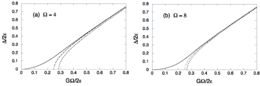
FIG. 1.: Pairing gaps (in units of $2\epsilon$) as a function of $G\Omega/(2\epsilon)$ for $\Omega=$ 4 (a) and 8 (b). The dotted line denotes the BCS gap $\Delta$ obtained including the self-energy term. The dashed line is the BCS result neglecting the self-energy term. The solid line stands for the gap $\Delta_{\rm LN}$ given by the LN method.

The gaps obtained within the BCS approximation and LN method using Eqs. (21) and (28) for $\Omega=$ 4 and 8 are plotted against the interaction parameter $G\Omega/(2\epsilon)$ in Fig. 1. With decreasing the interaction, the BCS gap $\Delta$ decreases and collapses at $G_{\rm cr}$, whose value for the case when the self-energy term is neglected is smaller than that obtained including the self-energy term. The LN gap $\Delta_{\rm LN}$, on the contrary, decreases monotonously with decreasing $G$ until $G=0$, where $\Delta_{\rm LN}$ vanishes, showing no signature of the superfluid-normal phase transition. Hence, by removing the particle number fluctuations, the LN method erases completely the odd behavior of the BCS gap characterized by this phase transition. The system remains in the superfluid phase at all nonzero values of the pairing interaction. It is interesting to see that, due to the suppression of the self-energy term $-Gv^{2}$ by $4\lambda_{2}v^{2}$ in the LN method, the BCS gap without the self-energy correction is closer to the LN result than the BCS gap including this correction. By comparing Fig. 1 (a) and (b), we also see that the difference between two BCS versions (with and without the self-energy term) decreases significantly when the particle number increases.

IV QRPA (RPA), its renormalization, and combination with the LN method

The RPA ground state includes $2p2h$-, $4p4h$-, $6p6h$-, etc. excitations on top of the HF ground state. The RPA including the pairing correlations within the quasiparticle representation is usually referred to as the QRPA. The correlations in the QRPA ground state, therefore, are much richer than the $2p2h$-, $4p4h$-, etc. correlations in the “diffuse” (quasiparticle) ground state $|0\rangle_{\alpha}$ created by scattering of particle pairs within the BCS approximation. The LN method takes into account some $2p2h$-correlations beyond the BCS approximation by using the $\lambda_{2}\hat{N}^{2}$ term. However, this method still uses the same BCS ground state $|0\rangle_{\alpha}$ since it approximately expresses the expectation value of the Hamiltonian with respect to the projected state in terms of that with respect to the BCS ground state [11]. The discussion below is conducted within the QRPA, where the RPA is obtained as the limit when $\Delta=$ 0. Consequently, we summarize also the main features of the renormalized QRPA, whose zero-pairing limit is the renormalized RPA. In the present two-level model, the QRPA works at $G\geq G_{\rm cr}$, while the RPA is applied at $G<G_{\rm cr}$.

A QRPA

The standard QRPA operators, called phonon operators, have the following form in the present two-level model

$$Q^{\dagger}_{\nu}=\sum_{j}(X_{j}^{(\nu)}{\cal A}_{j}^{\dagger}-Y_{j}^{(\nu)}{\cal A}_{j})~{},\hskip 22.76219ptQ_{\nu}=(Q_{\nu}^{\dagger})^{\dagger}~{},$$ (34)

The QRPA ground state $|0\rangle_{\rm Q}$ is defined as the vacuum for the phonon operator, i.e. $Q_{\nu}|0\rangle_{\rm Q}=0={}_{\rm Q}\langle 0|Q^{\dagger}_{\nu}$. The $0^{+}$ excited state $|0^{+}\rangle$ is obtained by acting $Q^{\dagger}_{\nu}$ on this vacuum, i.e. $|0^{+}\rangle=Q^{\dagger}_{\nu}|0\rangle_{\rm Q}$. The excitation energy $\omega_{\nu}$ of the state $|0^{+}\rangle$, and the amplitudes $X_{j}^{(\nu)}$ and $Y_{j}^{(\nu)}$ are found respectively as the eigenenergy and the components of the eigenvector of the QRPA equation, which is derived from the following equation of motion for the Hamiltonian (7):

$${}_{Q}\langle 0|[\delta Q,[H,Q^{\dagger}_{\nu}]]|0\rangle_{\rm Q}=\omega_{\nu}{}_{Q}\langle 0|[\delta Q,Q^{\dagger}_{\nu}]|0\rangle_{\rm Q}~{}.$$ (35)

In the standard way of derivation of the QRPA equations, the BCS equation is solved first. Then the a- and b-terms in the Hamiltonian (7) is replaced with the BCS result, which is $H_{\rm BCS}=\sum_{j}E_{j}{\cal N}_{j}$. Using the exact commutation relations (9), we see that, among the remaining terms of (7), which do not contribute in the BCS, the d-, h-, and q-terms start to contribute within the QRPA. The c-term and g-term do not contribute since, in the commutation with the phonon operators (34), the former gives a number, while the latter leads to the terms $\sim{\cal A}^{\dagger}_{j}{\cal A}^{\dagger}_{j^{\prime}}$, $\sim{\cal A}^{\dagger}_{j}{\cal A}_{j^{\prime}}$, and ${\cal N}_{j}(1-{\cal N}_{j^{\prime}}/\Omega_{j^{\prime}})$, which are left out by linearizing the equation of motion according to (35). Moreover, in order to obtain a set of QRPA equations, linear with respect to the $X_{j}^{(\nu)}$ and $Y_{j}^{(\nu)}$ amplitudes, another approximation called the quasiboson approximation is made, which implies that the following approximate commutation relation holds

$$[{\cal A}_{j},{\cal A}^{\dagger}_{j^{\prime}}]=\delta_{jj^{\prime}}~{},$$ (36)

instead of Eq. (9). The definition of phonon operators (34) and the quasiboson approximation (36) lead to the well-known normalization of the QRPA $X_{j}^{(\nu)}$ and $Y_{j}^{(\nu)}$ amplitudes

$$\sum_{j}[X_{j}^{(\nu)}X_{j}^{(\nu^{\prime})}-Y_{j}^{(\nu)}Y_{j}^{(\nu^{\prime})}]=\delta_{\nu\nu^{\prime}}$$ (37)

so that the phonon operators are bosons, i.e.:

$$[Q_{\nu},Q_{\nu^{\prime}}^{\dagger}]=\delta_{\nu\nu^{\prime}}$$ (38)

The quasiboson approximation (36) shows that the quasiparticle-pair operators ${\cal A}^{\dagger}_{j}$ and ${\cal A}_{j}$ behave like boson operators when interacting with each other. The effect of Pauli principle represented by the last term at the RHS of (9) is just ignored. The set of QRPA equations obtained in this way is written in the matrix form as

$${~{}~{}~{}A\hskip 22.76219ptB\choose-B~{}~{}-A}{X\choose Y}=\omega{X\choose Y}~{}.$$ (39)

The explicit form of the matrices $A$ and $B$ depend on the approximation. Below we compare the results obtained within the boson and fermion formalisms.

1 Boson formalism

The boson formalism is based on two following assumptions:

(a) It considers ${\cal A}_{j}^{\dagger}$ and ${\cal A}_{j^{\prime}}$ as ideal bosons ${\bf b}^{\dagger}_{j}$ and ${\bf b}_{j}$, respectively, according to the quasiboson approximation (36). The $j$-shell quasiparticle number operator ${\cal N}_{j}$ is then mapped onto a boson pair as

$${\cal N}_{j}=2{\bf b}^{\dagger}_{j}{\bf b}_{j}.$$ (40)

This mapping preserves the commutators (10). The Hamiltonian (7) can be then fully expressed in terms of the boson operators ${\bf b}^{\dagger}_{j}$ and ${\bf b}_{j}$.

(b) In deriving the QRPA equations according to (35), the q-term of the Hamiltonian (7) is neglected. This term is a special case of the so-called scattering term in the general Hamiltonian with a two-body residual interaction. For instance, when the residual interaction is separable, the q-term involves a sum of products of two scattering quasiparticle pairs $\sim B_{jj^{\prime}}^{\dagger}(LM)B_{j_{1}j_{1}^{\prime}}(L\widetilde{M})$, where $B_{jj^{\prime}}(LM)=-\sum_{mm^{\prime}}\langle jmj^{\prime}m^{\prime}|LM\rangle\alpha_{jm}^{\dagger}\alpha_{j^{\prime}\widetilde{m^{\prime}}}$ is the scattering quasiparticle-pair operator. The latter is equal to ${\cal N}_{j}/\sqrt{2j+1}$ when $L=0$. The scattering term is usually omitted in most of numerical calculations within QRPA for realistic nuclei in literature.

The boson mapping of the phonon operator (34) becomes

$$Q_{\nu}^{\dagger}\rightarrow\sum_{j}(X_{j}^{(\nu)}{\bf b}_{j}^{\dagger}-Y_{j}^{(\nu)}{\bf b}_{j})~{}.$$ (41)

The QRPA matrices $A_{jj^{\prime}}$ and $B_{jj^{\prime}}$ have the simple form:

$$A_{jj^{\prime}}=2E_{j}\delta_{jj^{\prime}}+d_{jj^{\prime}}~{},\hskip 22.76219ptB_{jj^{\prime}}=2h_{jj^{\prime}}~{},$$ (42)

which, in the present two-level model, become

$$A_{11}=A_{22}=G\Omega+\frac{\Delta^{2}}{2G\Omega}~{},$$ (43)

$$A_{12}=A_{21}=-\frac{\Delta^{2}}{2G\Omega}~{},$$ (44)

$$B_{11}=B_{22}=\frac{\Delta^{2}}{2G\Omega}~{},$$ (45)

$$B_{12}=B_{21}=G\Omega-\frac{\Delta^{2}}{2G\Omega}~{}.$$ (46)

The QRPA equations give one positive solution equal to

$$\omega_{\rm QRPA}^{(b)}=2\Delta~{},$$ (47)

while the spurious state associated with the non-conservation of particle number is located exactly at zero energy. We see that the energy of the first excited $0^{+}$ state above the phonon ground state $|0\rangle_{\rm Q}$ is just twice the pairing gap, the same for the lowest two-quasiparticle excitation above the quasiparticle ground state $|0\rangle_{\alpha}$ of a system with an even particle number.

In the normal-fluid phase ($\Delta$=0), the quasiparticle operator $\alpha_{jm}$ becomes the particle-($p$) creation or hole-($h$) destruction operator depending on whether the level is located above or below the Fermi level, namely

$$\alpha_{jm}^{\dagger}=\left\{\begin{array}[]{ll}a_{jm}^{\dagger}&\textrm{if $\epsilon_{j}>\lambda$}\\ -a_{j-m}&\textrm{if $\epsilon_{j}<\lambda$}\end{array}\right.$$ (48)

Therefore, the following boson mapping for operators $A_{j}^{\dagger}$ and $A_{j}$ holds

$$A_{j}^{\dagger}\rightarrow\left\{\begin{array}[]{ll}{\bf b}^{\dagger}_{j}&\textrm{if $\epsilon_{j}>\lambda$}\\ {\bf b}_{j}&\textrm{if $\epsilon_{j}<\lambda$}\end{array}\right.~{},\hskip 22.76219ptA_{j}\rightarrow\left\{\begin{array}[]{ll}{\bf b}_{j}&\textrm{if $\epsilon_{j}>\lambda$}\\ {\bf b}^{\dagger}_{j}&\textrm{if $\epsilon_{j}<\lambda$}\end{array}\right.~{},$$ (49)

The boson mapping for the number operator $N_{j}$ is given as

$$N_{j}=\left\{\begin{array}[]{ll}2{\bf b}_{j}^{\dagger}{\bf b}_{j}&\textrm{if $\epsilon_{j}>\lambda$}\\ 2(\Omega_{j}-{\bf b}_{j}^{\dagger}{\bf b}_{j})&\textrm{if $\epsilon_{j}<\lambda$}\end{array}\right.~{},$$ (50)

which preserves the commutation relations (5) and the particle number on the j-shell equal to $2\Omega_{j}$. The RPA matrices for the two-level model are

$$A_{11}=A_{22}=2(\epsilon-G\Omega)~{},\hskip 22.76219ptA_{12}=A_{21}=0~{}.$$ (51)

$$B_{11}=B_{22}=0~{},\hskip 22.76219ptB_{12}=B_{21}=-2G\Omega~{}.$$ (52)

They lead to the RPA phonon energy

$$\omega_{\rm RPA}^{(b)}=2\epsilon\sqrt{1-\frac{G}{G_{\rm cr}^{(b)}}}~{},\hskip 22.76219ptG_{\rm cr}^{(b)}=\frac{\epsilon}{2\Omega}~{}.$$ (53)

The critical value of $G_{\rm cr}^{(b)}$ where the RPA collapses is the same collapsing point of the BCS obtained without the self-energy term (Eqs. (23) and (24)). Therefore, in order to have the superfluid regime start at the same critical point, the gap $\Delta$ in Eqs. (43) – (47) should be calculated neglecting the self-energy term in the BCS equation (21). This gives

$$\Delta^{(b)}=G\Omega\sqrt{1-\bigg{(}\frac{\epsilon}{2G\Omega}\bigg{)}^{2}}~{}.$$ (54)

The phonon energies (47) and (53) are exactly those obtained for the first time in Ref. [18] using the space-variable technique and the gap $\Delta^{(b)}$ (54).

2 Fermion formalism

The fermion formalism does not use directly the quasiboson approximation (36). Instead, it employs the exact commutation relations (9) and (10) to rearrange the results of calculating the commutators $[H,{\cal A}^{\dagger}_{j}]$ and $[H,{\cal A}_{j}]$ into the normal order. Then, in the process of linearizing the equation of motion (35) the following “average” quasiboson approximation is used

$${~{}}_{\rm Q}\langle 0|[{\cal A}_{j},{\cal A}_{j^{\prime}}^{\dagger}]|0\rangle_{\rm Q}=\delta_{jj^{\prime}}~{},$$ (55)

assuming that the quasiparticle occupation number $n_{j}$ in the RPA ground state is zero, i.e.

$$n_{j}\equiv\frac{{}_{\rm Q}\langle 0|{\cal N}_{j}|0\rangle_{\rm Q}}{2\Omega_{j}}=0~{}.$$ (56)

The QRPA matrices are obtained in this way as

$$A_{jj^{\prime}}=2(E_{j}+2q_{jj})\delta_{jj^{\prime}}+d_{jj^{\prime}}~{},\hskip 22.76219ptB_{jj^{\prime}}=2(1-\frac{1}{\Omega_{j}}\delta_{jj^{\prime}})h_{jj^{\prime}}~{}.$$ (57)

Their explicit form in the two-level model is given as

$$A_{11}=A_{22}=G\Omega-\frac{\Delta^{2}}{G\Omega^{2}}+\frac{\Delta^{2}}{2G\Omega}~{},$$ (58)

$$A_{12}=A_{21}=-\frac{\Delta^{2}}{2G\Omega}~{},$$ (59)

$$B_{11}=B_{22}=-\frac{\Delta^{2}}{2G\Omega^{2}}+\frac{\Delta^{2}}{2G\Omega}~{},$$ (60)

$$B_{12}=B_{21}=G\Omega-\frac{\Delta^{2}}{2G\Omega}~{}.$$ (61)

The BCS equation (21) for the gap $\Delta$ includes the self-energy term. The $4q_{jj}\delta_{jj^{\prime}}$-term in the expression for $A_{jj}$ (Eqs. (57) and (58)) appears due to the use of the exact commutation relation (10) to calculate the commutator between the q-term of the Hamiltonian (7) and ${\cal A}^{\dagger}_{j}$ (or ${\cal A}_{j}$) as follows:

$$\sum_{j_{1}j_{1}^{\prime}}q_{j_{1}j_{1}^{\prime}}[{\cal N}_{j_{1}}{\cal N}_{j_{1}^{\prime}},{\cal A}^{\dagger}_{j}]=4q_{jj}{\cal A}^{\dagger}_{j}+4\sum_{j^{\prime}}q_{jj^{\prime}}{\cal A}^{\dagger}_{j}{\cal N}_{j^{\prime}}~{}.$$ (62)

The last term at the RHS of (62) does not contribute in the linearization within the QRPA. The first term leads to the above-mentioned 4$q_{jj}\delta_{jj^{\prime}}$-term. It is worthwhile to notice that, if one rearranges the quasiparticle operators in the q-term of (7) to the normal order as

$$\sum_{jj^{\prime}}q_{jj^{\prime}}{\cal N}_{j}{\cal N}_{j^{\prime}}=\sum_{j}q_{jj}{\cal N}_{j}-\sum_{jmj^{\prime}m^{\prime}}q_{jj^{\prime}}\alpha_{jm}^{\dagger}\alpha_{j^{\prime}m^{\prime}}^{\dagger}\alpha_{jm}\alpha_{j^{\prime}m^{\prime}}~{},$$ (63)

and then drops the last term at the RHS (although there is no rigorous justification for doing so), the remaining term in the commutation with ${\cal A}^{\dagger}_{j}$ gives

$$\sum_{j_{1}j_{1}^{\prime}}q_{j_{1}j_{1}^{\prime}}[{\cal N}_{j_{1}}{\cal N}_{j_{1}^{\prime}},{\cal A}^{\dagger}_{j}]\simeq\sum_{j^{\prime}}q_{j^{\prime}j^{\prime}}[{\cal N}_{j^{\prime}},{\cal A}^{\dagger}_{j}]=2q_{jj}{\cal A}_{j}^{\dagger}~{},$$ (64)

i.e. just the half of the first term at the RHS of Eq. (62). This explains the difference between Eq. (58) above and Eq. (38) of Ref. [6] by a factor of 2 in the denominator of the second term at their RHS.

The energy of the first $0^{+}$ excited state $\omega$ obtained solving the QRPA equation with the matrices (58) – (61) has the form

$$\omega_{1}=2\Delta\sqrt{\bigg{(}1-\frac{3}{4\Omega}\bigg{)}\bigg{(}1-\frac{\Delta^{2}}{4G^{2}\Omega^{3}}\bigg{)}}\hskip 8.53581pt~{}.$$ (65)

The energy of the spurious state in this case is imaginary. If one uses the approximation (64) instead of (62), the positive solution is given by Ref. [6] as:

$$\omega_{01}=2\Delta\sqrt{1-\frac{1}{2\Omega}}~{},$$ (66)

while the energy of the spurious state is exactly zero. Neglecting the q-term in (7) yields the energy of the first $0^{+}$ state as

$$\omega_{0}=2\Delta\sqrt{\bigg{(}1-\frac{1}{4\Omega}\bigg{)}\bigg{(}1+\frac{\Delta^{2}}{4G^{2}\Omega^{3}}\bigg{)}}~{}.$$ (67)

There are two features of the fermion formalism, which are worth noticing here. The fact that in the process of linearizing the equation of motion, the exact commutation relations (9) and (10) have been used to calculate the commutators $[H,{\cal A}^{\dagger}_{j}]$ and $[H,{\cal A}_{j}]$ does not reduce matrices (57) by setting $q_{jj^{\prime}}=$ 0 to those given within the boson formalism (42). The difference in $B_{jj}$ still remains. Another feature is that, when the q-term in (7) is omitted, the spurious mode in the fermion formalism is shifted to a positive value equal to

$$\omega_{0}^{s}=\Delta\sqrt{\frac{1}{\Omega}\bigg{(}1-\frac{\Delta^{2}}{4G^{2}\Omega^{3}}\bigg{)}}~{}.$$ (68)

However it is much smaller than the pairing gap $\Delta$ especially at large $\Omega$, therefore, remains well-isolated. Comparing Eqs. (65) – (67) with the boson energy $\omega_{\rm QRPA}^{(b)}$ (Eq. (47)), it is easy to see that

$$\omega_{1}<\omega_{01}<\omega_{0}<\omega_{\rm QRPA}^{(b)}=2\Delta~{}.$$ (69)

The ground-state energy is now calculated following Refs. [1, 6] as

$$E_{\rm QRPA}=E_{\rm BCS}+\frac{1}{2}[\omega-(A_{11}+A_{22})]~{}.$$ (70)

In the limit of zero gap, the $pp$-RPA equation is obtained from the QRPA equation discussed above putting $\Delta=$ 0, $v=v_{1}=u_{2}=$1, $u=u_{1}=v_{2}=0$. The solution of this RPA equation is decoupled into the addition and removal modes, which have been discussed in detail in Ref. [2, 6]. In the present two-level model, these two sets of equations can be written in one matrix equation as

$${A_{11}\hskip 22.76219ptB_{12}\choose B_{12}\hskip 22.76219ptA_{22}}{R_{p}^{(\tau)}\choose R_{h}^{(\tau)}}={1\hskip 22.76219pt0\choose 0~{}~{}-1}{R_{p}^{(\tau)}\choose R_{h}^{(\tau)}}\omega_{\tau}~{},\hskip 22.76219pt(\tau=~{}1,~{}2~{})~{},$$ (71)

where

$$A_{11}=\epsilon+2\lambda+2G-G\Omega~{},\hskip 22.76219ptA_{22}=\epsilon-2\lambda-G\Omega~{},\hskip 22.76219ptB_{12}=G\Omega~{},$$ (72)

and $R_{p}^{(1)}=X_{\rm a}$ , $R_{h}^{(1)}=Y_{\rm a}$ , $R_{p}^{(2)}=Y_{\rm r}$ , $R_{h}^{(2)}=X_{\rm r}$ , $\omega_{1}=\omega_{\rm a}$ , and $\omega_{2}=-\omega_{\rm r}$ . The energies $\omega_{\rm a}$ and $\omega_{\rm r}$ are found as

$$\omega_{\rm a}=-G-2\lambda\pm\sqrt{(\epsilon+G)(\epsilon+G-2G\Omega)}~{}.$$ (73)

$$\omega_{\rm r}=G+2\lambda\pm\sqrt{(\epsilon+G)(\epsilon+G-2G\Omega)}~{},$$ (74)

where only the sign $+$ in front of the square roots corresponds to the positive values for these energies. Here we still keep the factor $\pm 2\lambda$, which is useful to connect the RPA solutions with the QRPA one at the critical point $G=G_{\rm cr}$, where 2$\lambda=-G_{\rm cr}$ according to Eq. (20).

In order make a comparison with the boson formalism, where there is only one boson state, we apply the sum-rule method, representing the RPA phonon operator as

$$Q^{\dagger}=Q_{\rm a}^{\dagger}+Q_{\rm r}^{\dagger}~{}.$$ (75)

The RPA ground-state wave function $|\rm{RPA}\rangle$ can be written as a direct product of the ground-state wave functions of the (orthogonal) additional and removal modes

$$|\rm{RPA}\rangle=|0\rangle_{\rm a}\otimes|0\rangle_{\rm r}~{}.$$ (76)

Using the Thouless theorem for the energy-weighted sum rule ${\cal S}_{1}$  [2] with respect to the phonon operator $Q^{\dagger}$ (75)

$${\cal S}_{1}\equiv\sum_{i}\omega_{\rm RPA}^{(i)}|\langle\nu_{i}|Q^{\dagger}|{\rm RPA}\rangle|^{2}=\frac{1}{2}\langle{\rm HF}|[Q^{\dagger},[H,Q^{\dagger}]]|{\rm HF}\rangle~{},$$ (77)

it is easy to see that the LHS of Eq. (77) is equal $\omega_{\rm RPA}$ since $|\nu_{i}\rangle=Q^{\dagger}|{\rm RPA}\rangle$ ($i=$ 1), while the RHS is equal to

$\displaystyle\frac{1}{2}\bigg{[}\langle{\rm HF}|[Q_{\rm a}^{\dagger},[H,Q_{\rm a}^{\dagger}]]|{\rm HF}\rangle+\langle{\rm HF}|[Q_{\rm r}^{\dagger},[H,Q_{\rm r}^{\dagger}]]|{\rm HF}\rangle\bigg{]}=$

$$\omega_{\rm a}|\langle\nu_{\rm a}|Q^{\dagger}_{\rm a}|{\rm RPA}\rangle|^{2}+\omega_{\rm r}|\langle\nu_{\rm r}|Q^{\dagger}_{\rm r}|{\rm RPA}\rangle|^{2}=\omega_{\rm a}|\langle\nu_{\rm a}|\nu_{\rm a}\rangle|^{2}+\omega_{\rm r}|\langle\nu_{\rm r}|\nu_{\rm r}\rangle|^{2}=\omega_{\rm a}+\omega_{\rm r}~{}.$$ (78)

(The crossing terms $\langle{\rm HF}|[Q_{\rm i}^{\dagger},[H,Q_{\rm i^{\prime}}^{\dagger}]]|{\rm HF}\rangle$ ($i\neq i^{\prime}$) vanish as can be easily checked using $\langle i|i^{\prime}\rangle=\delta_{ii^{\prime}}$). Therefore

$$\omega_{\rm RPA}=\omega_{\rm a}+\omega_{\rm r}~{}.$$ (79)

The ground-state energy is then given by

$$E_{\rm RPA}=E_{\rm HF}+\frac{1}{2}(\omega_{\rm RPA}-A_{11}-A_{22})=\sqrt{(\epsilon+G)(\epsilon+G-2G\Omega)}-(\epsilon-G\Omega+G)~{},$$ (80)

which is exactly the same expression obtained previously in Eq. (45) of Ref. [6].

The energies of the ground-state and the first $0^{+}$ state obtained within the fermion formalism of RPA and QRPA for $\Omega=$ 4 are compared with the exact energies in Fig. 2. The figure shows that, in the superfluid regime, except for the region close to the critical point $G=G_{\rm cr}$ where the QRPA collapses, the approximation (64) fits the exact result for the ground-state energy better than (62). For the energy of the first $0^{+}$ state, both of the QRPA versions, which include the q-term of the Hamiltonian (7) give practically the same values. However, they are obviously smaller compared to the exact solution. This discrepancy increases with increasing the interaction. From Eqs. (65) – (67) we found that, in the limit of infinite $G$ the solution $\omega_{0}$ (q-term neglected) becomes $2\Delta\sqrt{1-1/4\Omega}\simeq 3.88\Delta$, while the solutions $\omega_{1}$ based on the approximation (62), and $\omega_{10}$ based on (64) [6] are equal to $0.96\omega_{0}$ and $0.93\omega_{0}$, respectively. The only QRPA approximation that fits well the exact results for both of the ground-state and excited-state energies the one, which neglects the q-term of the Hamiltonian (7). The results within this approximation practically coincide with the exact ones at large $G$. The RPA energy $\omega_{\rm RPA}=\omega_{\rm a}+\omega_{\rm r}$ of the first ${0}^{+}$ state exhibits the well-known behavior. It decreases with increasing $G$ and collapses at the same critical point $G=G_{\rm cr}$, from which the the normal-fluid phase ceases to exist, and the superfluid phase begins. Meanwhile, the exact solution for the first excited state has only a bending in this region, showing no signature of such phase transition. For the ground-state energy the exact result shows a completely smooth curve, while the critical point is clearly seen in the approximations.

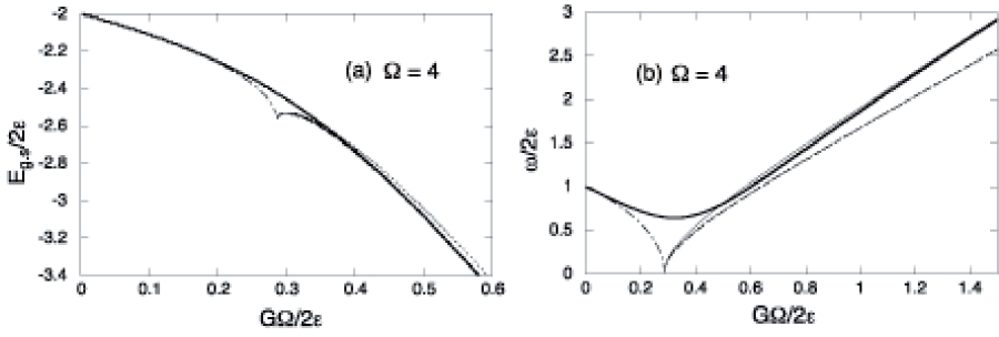
FIG. 2.: The ground-state energy (a) and energy of the first excited state (b) (in units of $2\epsilon$) as a function of $G\Omega/(2\epsilon)$. The thick solid line is the exact result. The thin solid line shows the QRPA result neglecting the q-term in the Hamiltonian (7). The dashed line denotes the QRPA result of Ref. [6]. The dotted line stands for the result obtained using the matrices (58) – (61). The dash-dotted line represents the RPA result.

As shown in Fig. 3 for $\Omega=$ 4, the QRPA energy $\omega_{0}$ obtained without the q-term of (7), and the RPA energy $\omega_{\rm RPA}$ also match well the solutions of the boson formalism, especially after shifting $G_{\rm cr}=G_{\rm cr}^{(b)}$ in the latter to the value of $\epsilon/(2\Omega-1)$ used in the fermion formalism due to the inclusion of the self-energy term (Eq. (24)).

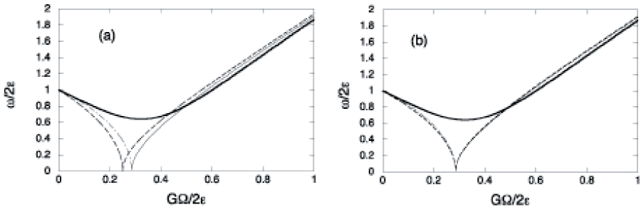
FIG. 3.: The energy of the first ${0}^{+}$ state (in units of $2\epsilon$) given by the boson formalism (dashed line) in comparison with those obtained within the QRPA (thin solid line) neglecting the q-term of the Hamiltonian (7), RPA as the sum $\omega_{\rm a}+\omega_{\rm r}$ (dash-dotted line), and the exact solution (thick solid line) for $\Omega=$ 4. In (a) the boson energy [Eqs. (47) and (53)] has been obtained using $G_{\rm cr}=G_{\rm cr}^{(b)}=\epsilon/2\Omega$ (neglecting the self-energy term). In (b) the boson energy has been calculated using the value $G_{\rm cr}=\epsilon/(2\Omega-1)$ obtained including the self-energy term.

B Renormalized QRPA

The collapse of the BCS approximation and QRPA (RPA) has the same origin of neglecting the Pauli principle between quasiparticle pairs operators in the BCS approximation (26) and the quasiboson approximation strictly (36) or in average (55). The LN method approximately corrects this inconsistency within the BCS approximation. For the QRPA this is done by the renormalized QRPA.

The essence of the renormalized QRPA is to replace the quasiboson approximation in the form of Eqs. (36) or (55) with the average value of the commutator

$$\langle\widetilde{0}|[{\cal A}_{j},{\cal A}^{\dagger}_{j^{\prime}}]|\widetilde{0}\rangle=D_{j}\delta_{jj^{\prime}}~{},\hskip 22.76219ptD_{j}=1-2n_{j}~{},$$ (81)

in a new ground state $|\widetilde{0}\rangle$, where the correlations beyond the QRPA due to the fermion structure of the quasiparticle pairs ${\cal A}^{\dagger}_{j}$ and ${\cal A}_{j}$ are taken into account, namely

$$n_{j}=\frac{1}{2\Omega_{j}}\langle\widetilde{0}|{\cal N}_{j}|\widetilde{0}\rangle\neq 0~{},$$ (82)

instead of the assumption (56). The phonon operators are renormalized as

$${\cal Q}_{\nu}=\sum_{j}\frac{1}{\sqrt{D_{j}}}({\cal X}_{j}^{(\nu)}{\cal A}^{\dagger}_{j}-{\cal Y}^{(\nu)}_{j}{\cal A}_{j})~{},\hskip 22.76219pt{\cal Q_{\nu}}=({\cal Q}_{\nu}^{\dagger})^{\dagger}~{},$$ (83)

so that the condition for phonons to be bosons within the correlated ground state $|\widetilde{0}\rangle$

$$\langle\widetilde{0}|[{\cal Q}_{\nu},{\cal Q}^{\dagger}_{\nu^{\prime}}]|\widetilde{0}\rangle=\delta_{\nu\nu^{\prime}}~{}$$ (84)

leads to the same normalization condition for the amplitudes ${\cal X}_{j}^{(\nu)}$ and ${\cal Y}_{j}^{(\nu)}$ as that of the QRPA, i.e. $\sum_{j}({\cal X}_{j}^{(\nu)}{\cal X}_{j}^{(\nu^{\prime})}-{\cal Y}_{j}^{(\nu)}{\cal Y}_{j}^{(\nu^{\prime})})=\delta_{\nu\nu^{\prime}}~{}.$ The factor $D_{j}$ is calculated according to the approximation in Ref. [16] as

$$D_{j}=\frac{1}{1+({\cal Y}_{j}^{(\nu)})^{2}/{\Omega_{j}}}.$$ (85)

The renormalized-QRPA matrices $A_{jj^{\prime}}$ and $B_{jj^{\prime}}$ are given as

$$A_{jj^{\prime}}=2(E_{j}+2q_{jj})\delta_{jj^{\prime}}+4\sum_{j"}\Omega_{j^{\prime\prime}}q_{j^{\prime}j^{\prime\prime}}(1-D_{j^{\prime\prime}})+D_{j}d_{jj^{\prime}}~{},$$ (86)

$$B_{jj^{\prime}}=2(D_{j}-\frac{1}{\Omega_{j}}\delta_{jj^{\prime}})h_{jj^{\prime}}~{}.$$ (87)

Since only the omission of the q-term in (7) within the QRPA reproduces well the exact solution in the present two-level model at large values of $G$, we discuss below only the case when $q_{jj^{\prime}}=$0. The renormalized QRPA matrices in this case read

$$A_{11}=A_{22}=G\Omega(2-D)+\frac{D\Delta^{2}}{2G\Omega^{2}}~{},\hskip 22.76219ptA_{12}=A_{21}=-\frac{\Delta^{2}}{2G\Omega}(4-3D)~{},$$ (88)

$$B_{11}=B_{22}=-\frac{\Delta^{2}}{2G\Omega^{2}}+\frac{D\Delta^{2}}{2G\Omega}~{},\hskip 22.76219ptB_{12}=B_{21}=D(G\Omega-\frac{\Delta^{2}}{2G\Omega})~{}.$$ (89)

The energy of the first excited $0^{+}$ state is found as

$$\omega_{\rm RQRPA}=2\Delta\sqrt{\bigg{[}\bigg{(}D-\frac{1}{4\Omega}\bigg{)}+\frac{G^{2}\Omega^{2}(1-D)}{\Delta^{2}}\bigg{]}\bigg{(}1+\frac{\Delta^{2}}{4G^{2}\Omega^{3}}\bigg{)}}~{},$$ (90)

By setting $D_{j}=$ 1 ($n_{j}=$ 0) in Eqs. (88) – (90), the QRPA limit in Eqs. (58) – (61) (without the second term at the RHS of (58) since the q-term is neglected), and $\omega_{0}$ given by Eq. (67) are recovered . The ground-state energy is calculated using Eq. (70), using the energy $\omega_{\rm RQRPA}$ given by Eq. (90) and the matrices $A_{11}=A_{22}$ given by Eq. (88).

The renormalized RPA matrices ($G<G_{\rm cr}$) are given as

$$A_{11}=\epsilon+2G-DG\Omega~{},\hskip 22.76219ptA_{22}=\epsilon-DG\Omega~{},\hskip 22.76219ptA_{12}=A_{21}=0~{},$$ (91)

$$B_{11}=B_{22}=0~{},\hskip 22.76219ptB_{12}=B_{21}=DG\Omega~{}.$$ (92)

The positive renormalized RPA phonon energies are found as

$$\widetilde{\omega}_{\rm a}=-G-2\lambda+\sqrt{(\epsilon+G)(\epsilon+G-2DG\Omega)}~{}.$$ (93)

$$\widetilde{\omega}_{\rm r}=G+2\lambda+\sqrt{(\epsilon+G)(\epsilon+G-2DG\Omega)}~{},$$ (94)

$$\omega_{\rm RRPA}=\widetilde{\omega}_{\rm a}+\widetilde{\omega}_{\rm r}=2\sqrt{(\epsilon+G)(\epsilon+G-2DG\Omega)}~{},$$ (95)

and the ground-state energy is

$$E_{\rm RRPA}=\sqrt{(\epsilon+G)(\epsilon+G-2DG\Omega)}-(\epsilon+G-DG\Omega)~{}.$$ (96)

As has been shown in Ref. [16], the presence of the factor $D$ in the renormalized RPA matrices reduces the interaction in such a way that the critical point where the RPA collapses is completely washed out. The energy $\widetilde{\omega}_{\rm a}$, $\widetilde{\omega}_{\rm r}$, and consequently, $\omega_{\rm RRPA}$ are always real. As for the renormalized QRPA, the presence of the pairing gap $\Delta$ makes it still collapse if $\Delta$ is calculated within the BCS (Eq. (21), but it is no longer the case if the LN pairing gap $\Delta_{\rm LN}$ (28) is used.

C LN-method + renormalized RPA (renormalized QRPA)

We have seen in the preceding sections that the LN-method allows us to avoid the phase transition of the BCS approximation, the QRPA without the q-term in (7) provides us with the best fit of the exact results for the energies of the ground state and the first excited ${0}^{+}$ state, while the renormalized RPA is known to smear out the collapse of the RPA due to the violation of the Pauli principle within the quasiboson approximation [16]. Therefore, in order to avoid the phase transition and to give at the same time a good description for both of the energies of the ground state as well as the fist excited ${0}^{\dagger}$ state, we propose here the following recipe.

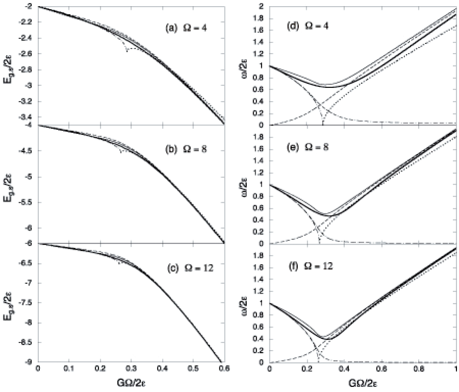
FIG. 4.: The energies of the ground state (left panels) and of the first ${0}^{+}$ excited state (right panels) (in units of $2\epsilon$) at several values of $\Omega$. The thick solid line is the exact result. The dotted line is the QRPA result using the matrices (58) – (61). The dash-dotted line denotes the RPA result. In (a) – (c): the dashed line shows the LN result, while the thin solid line represents the ground-state energy calculated according to (ii) of Section IV C. In (d) – (f): the dashed line stands for renormalized QRPA result using the LN pairing gap and neglecting the q-term in (7); the double-dash-dotted line represents the renormalized RPA results; the thin solid line is the energy $\omega_{0^{+}}$ according to Eq. (97).

i) The QRPA equations (without the q-term in (7)) are solved using the pairing gap $\Delta_{\rm LN}$ (28) found in the LN method.

ii) The ground state energy is calculated using Eq. (70), in which the LN pairing gap $\Delta_{\rm LN}$ is used instead of the BCS gap $\Delta$ (21) and the renormalized QRPA matrices given by Eq. (88) are used instead of Eq. (58).

iii) The first excited $0^{+}$ state is presented as a mixed state of those obtained within the renormalized RPA and renormalized QRPA (in (i)). Applying the sum-rule method and following a derivation similar to Eqs. (76) – (78), we find that the energy $\omega_{0^{+}}$ of this mixed state is the sum of the renormalized RPA and renormalized QRPA energies, namely

$$\omega_{0^{+}}=\omega_{\rm RRPA}+\omega_{\rm RQRPA}~{},$$ (97)

where $\omega_{\rm RRPA}$ and $\omega_{\rm QRPA}$ are given by Eqs. (95) and (90), respectively, with $\Delta_{\rm LN}$ used in the latter. The results obtained using this recipe will be referred to as the combined results.

The combined results for ground state energy and the energy of the first excited $0^{+}$ state are presented as thin solid lines in Fig. 4 at several values of $\Omega$ in comparison with the exact results and those of RPA, QRPA and their renormalized versions. The result obtained within the renormalized RPA and the combined result (i) for the energy of the first excited $0^{+}$ state show that the superfluid-normal phase transition is completely washed out. For the ground-state energy, the combined result (ii) is closer to the exact one compared to the LN result in the weak-coupling region ($G\ll G_{\rm cr}$) and in the region around $G_{\rm cr}$. It coincides with the LN and exact results in the strong-coupling region ($G\gg G_{\rm cr}$) (See the thin lines in Fig. 4 (a) – (c)). The combined result (iii) agrees reasonable well with the exact results (See the thin lines in Fig. 4 (d) – (f)), especially for larger $\Omega$. Hence, this numerical test confirms the validity of the assumption (iii) that the exact excited $0^{+}$ state may be considered as a mixed state where both of the normal and superfluid phases coexist at $G\neq$ 0. The weak-coupling region is dominated by the normal-fluid phase, where the energy $\omega_{0^{+}}$ of the first excited $0^{+}$ state decreases monotonously with increasing the pairing interaction $G$. The strong-coupling region is dominated by the superfluid phase, in which $\omega_{0^{+}}$ increases with increasing $G$.

V Conclusions

In this work, a schematic model of two symmetric levels interacting via a pairing force has been used to test several well-known approximations by calculating the ground-state energy and the energy $\omega_{0^{+}}$ of the first excited $0^{+}$ state. Results obtained within the BCS approximation, LN method, boson and fermion formalisms for RPA and QRPA, renormalized RPA, and renormalized QRPA have been analyzed in details. It is shown that the common version of the QRPA, which neglects the scattering term (the q-term of the Hamiltonian (7)) and the boson formalism give the closest results to the exact ones for both of the ground-state energy and $\omega_{0^{+}}$ at the values of the pairing interaction parameter $G\gg G_{\rm cr}$. Meanwhile the QRPA version used in Ref. [6] as well as the QRPA using the exact commutation relations between quasiparticle-pair operators to treat the scattering term do not describe well the energy of the first excited $0^{+}$ state at large $G$.

A recipe has been proposed which combines the results obtained within the LN method for the pairing gap $\Delta_{\rm LN}$, the renormalized RPA, and the renormalized QRPA neglecting the last term (q-term) of the Hamiltonian (7). The combined results agree reasonably well with the exact ones for both of the ground-state energy and $\omega_{0^{+}}$, showing no signature of a sharp superfluid-normal phase transition. The agreement is better at a larger particle number. The results suggest that the exact excited $0^{+}$ state can be decomposed approximately into two components, which correspond to the normal and superfluid regimes, respectively. The weak-coupling region is dominated by the normal-fluid phase, while the strong-coupling region - by the superfluid phase. Since the proposed scheme is based on rather simple, well-known, and numerically accessible approximations, its future extension toward an application in realistic nuclei may be useful.

For a more self-consistent approach, one can derive the set of RPA equations using the Hamiltonian (7) with the coefficients $u_{j}$, $v_{j}$, $X_{j}^{(\nu)}$ and $Y_{j}^{(\nu)}$ left as variational parameters when minimizing the average energies over the ground state and the first excited $0^{+}$ state. This may serve as a goal of the future study.

REFERENCES

• [1] D.J. Rowe, Phys. Rev. 175, 1293 (1968); Rev. Mod. Phys. 40, 153 (1968); Nucl. Phys. A107, 99 (1968).
• [2] P. Ring and P. Schuck, The nuclear many-body problem, (Springer-Verlag, New-York, 1980).
• [3] J. Toivanen and J. Suhonen, Phys. Rev. Lett. 75, 410 (1995); J.G. Hirsch, P.O. Hess, and O. Civitarese, Phys. Rev. C 54, 1976 (1996); Phys. Lett. B 390, 36 (1997); M. Sambataro and J. Suhonen, Phys. Rev. C 56, 782 (1997); M. Sambataro and N. Dinh Dang, Phys. Rev. C 59, 1422 (1999); J. Dukelsky, G. Röpke, and P. Schuck, Nucl. Phys. A 628, 17 (1998); J. Dukelsky and P. Schuck, Phys. Lett. B 464, 164 (1999).
• [4] A. Volya, B.A. Brown, and V. Zelevinsky, Phys. Lett. B 509, 37 (2001); J. Engel, S. Pittel, M. Stoitsov, P. Vogel, and J. Dukelsky, Phys. Rev. C 55, 1781 (1997).
• [5] K. Hagino and G.F. Bertsch, Phys. Rev. C 61, 024307 (2000).
• [6] K. Hagino and G.F. Bertsch, Nucl. Phys. A 679, 163 (2000).
• [7] I. Stetscu and C.W. Johnson, arXiv:nucl-th/0205029.
• [8] N. Ullah and D.J. Rowe, Phys. Rev. 188, 1640 (1969).
• [9] M. Sambataro, Phys. Rev. C 52, 3378 (1995).
• [10] H.J. Lipkin, Ann. of. Phys. 31, 525 (1960); Y. Nogami and I.J. Zucker, Nucl. Phys. 60, 203 (1964); Y. Nogami, Phys. Lett. 15, 335 (1965); J.F. Goodfellow and Y. Nogami, Can. J. Phys. 44, 1321 (1966).
• [11] H.C. Pradhan, Y. Nogami, and J. Law, Nucl. Phys. A 201. 357 (1973).
• [12] K. Hara, Prog. Theor. Phys. 32, 88 (1964); K. Ikeda, T. Udagawa, and H. Yamamura, ibid. 33, 22 (1965).
• [13] A. Klein, R.M. Dreizler, and R.E. Johnson, Phys. Rev. 171, 1216 (1968).
• [14] P. Schuck and S. Ethofer, Nucl. Phys. A212, 269 (1973); J. Dukelsky and P. Schuck, ibid. A512, 446 (1990).
• [15] F. Krmpotic, T.T.S. Kuo, A. Mariano, E.J.V. Passos, A.F.R. de Toledo Piza, Nucl. Phys. A 612, 223 (1997).
• [16] F. Catara, N. Dinh Dang, and M. Sambataro, Nucl. Phys. A579, 1 (1994).
• [17] N.D. Dang and A. Arima, Phys. Rev. C 62, 024303 (2000), N. Dinh Dang and V. Zelevinsky, Phys. Rev. C 64, 064319 (2001).
• [18] J. Högaasen-Feldman, Nucl. Phys. 28, 258 (1961).
• [19] R.W. Richarson and N. Sherman, Nucl. Phys, 52, 221 (1964).
• [20] N. Dinh Dang, Z. Phys. A 335, 253 (1990).
• [21] M. Rho and J.O. Rasmussen, Phys. Rev. 135 B1295, (1964).