Time scales for fission at finite temperature

Abstract

The concept of the ”transient effect” is examined in respect of a ”mean first passage time”. It is demonstrated that the time the fissioning system stays inside the barrier is much larger than suggested by the transient time, and that no enhancement of emission of neutrons over that given by Kramers’ rate formula ought to be considered.

Keywords: Decay rate, transient effect, mean first passage time
PACS: 05.60-k, 24.10.Pa, 24.60.Dr, 24.75.+i

”Symposium on Nuclear Clusters”,
Rauischholzhausen, Germany, 5-9 August 2002

1 Introduction

Fission at finite thermal excitation is characterized by the evaporation of light particles and $\gamma$’s. Any description of such a process must rely on statistical concepts, both with respect to fission itself as well as with respect to particle emission. For decades it has been customary to describe experiments in terms of particle and fission widths, where the former, $\Gamma_{n}$, is identified through the evaporation rate and the latter $\Gamma_{f}$ is given by the Bohr-Wheeler formula $\Gamma_{f}\equiv\Gamma_{\rm{BW}}$ for the fission rate. Often in the literature this is referred to as the ”statistical model”. It was only in the 80’s that discrepancies of this procedure with experimental evidence was encountered: Sizably more neutrons were seen to accompany fission events than given by the ratio $\Gamma_{n}/\Gamma_{\rm{BW}}$ (for a review see e.g. [1]). It was then that one recalled Kramers’ old objection [2] against the Bohr-Wheeler formula. Indeed, in this seminal paper he pointed to the deficiency of the picture of Bohr and Wheeler in that it discards the influence of couplings of the fission mode to the nucleonic degrees of freedom. Such couplings will in general reduce the flux across the barrier as the energy in the fission degree of freedom $Q$ may be diminished and fall below the barrier.

In Kramers’ picture this effect is realized through the presence of frictional and fluctuating forces (intimately connected to each other by the fluctuation dissipation theorem). For not too weak dissipation Kramers’ rate formula writes

$$\Gamma_{\rm{K}}=\frac{\hbar\varpi_{\rm{a}}}{2\pi}\exp\left(-\frac{E_{\rm{b}}}{T}\right)\,\left(\sqrt{1+\eta_{\rm{b}}^{2}}-\eta_{\rm{b}}\right)=\frac{\hbar}{\tau_{\rm{K}}}=\hbar R_{\rm{K}}.$$ (1)

Here, $T$ and $E_{\rm{b}}$ stand for temperature and barrier height, $\varpi_{\rm{a}}$ for the frequency of the motion in the (only) minimum at $Q=Q_{\rm{a}}$ and $\eta_{\rm{b}}=(\gamma/(2M\varpi))_{\rm{b}}$ for the dissipation strength at the barrier (at $Q=Q_{\rm{b}}$) with $\gamma$ being the friction coefficient and $M$ the inertia. For the sake of simplicity we will assume these coefficients not to vary along the fission path; otherwise the formula must be modified [3]. For vanishing dissipation strength (1) reduces to the Bohr-Wheeler formula (simplified to the case that the equilibrium of the nucleons can be parameterized by a temperature).

Commonly, formula (1) is derived in a time dependent picture solving the underlying Fokker-Planck equation for special initial conditions with respect to the time dependence of the distribution function. The initial condition is intimately related to the condition of a compound reaction, in that the decay process is assumed to be independent of how the compound nucleus is produced. In this spirit one does not need to care for the truly initial stages of the reaction. One simply assumes the system to be located initially around the ground state minimum $Q=Q_{\rm{a}}$ of the static energy. However, there still is room for the precise definition, as the system may or may not be in (quasi-)equilibrium with respect to the fission degree of freedom $Q$ — which for large damping belongs to the slowest modes present. Since the corresponding momentum may safely be assumed to relax much faster one may also let the system start sharply at $Q=Q_{\rm{a}}$ with a Maxwell distribution in $P$. In any case, for the current across the barrier it takes some finite time to build up. This apparent delay of fission was taken [4, 5] as an indication for additional possibilities to emit light particles beyond the measure given by $\Gamma_{n}/\Gamma_{\rm{K}}\,>\,\Gamma_{n}/\Gamma_{\rm{BW}}$.

In case that the full process is studied in a time dependent picture both for fission as well as for particle emission, as done in the typical Langevin codes [6], such an effect is included automatically. Problems arise, however, if one tries to imitate this delay in statistical codes which are in use for analyzing experimental results. Such codes are based on time independent reaction theory. For this reason it is not obvious how this method may be reconciled with the picture of fission delay, the ”transient effect”. In the present note we like to shed some light on this problem by exploiting the concept of a ”mean first passage time” (MFPT).

2 Time dependent current across the barrier

Solutions of the transport equation require appropriate boundary conditions for the coordinate $Q$ (and $P$ if present). For the solutions discussed above the boundary conditions are chosen to make sure that the distribution vanishes at infinity. Calculations of the current $j(t)$ across the barrier then typically imply a behavior as exhibited in Fig.1 for different initial conditions. In all cases the asymptotic value of $j_{\rm{b}}(t)$ is seen to behave like $\Gamma_{\rm{K}}\exp(-\Gamma_{\rm{K}}\,t/\hbar)$. The differences at short times are due to the following choices:

(i) For the dashed curves the system starts out of equilibrium for both $Q$ and $P$; the curve on the left corresponds to the current at the barrier $j_{\rm{b}}(t)=j(Q_{\rm{b}},t)$ and the right one to that in the scission region $j_{\rm{sc}}(t)=j(Q_{\rm{sc}},t)$. The equilibrium is defined by the oscillator potential which approximates the $V(Q)$ around $Q_{\rm{a}}$.

(ii) For the fully drawn line the system starts at $Q_{\rm{a}}$ sharp with a Maxwell distribution in $P$. The obvious delay is essentially due to the relaxation of $Q$ to the quasi-equilibrium in the well. This feature is demonstrated on the right by the $t$-dependence of the width in $Q$ (as given by the average potential energy).

(iii) The dotted curve corresponds to an initial distribution which is also sharp in the momentum but centers at the finite value $\langle P\rangle_{t=0}=\sqrt{MT}$.

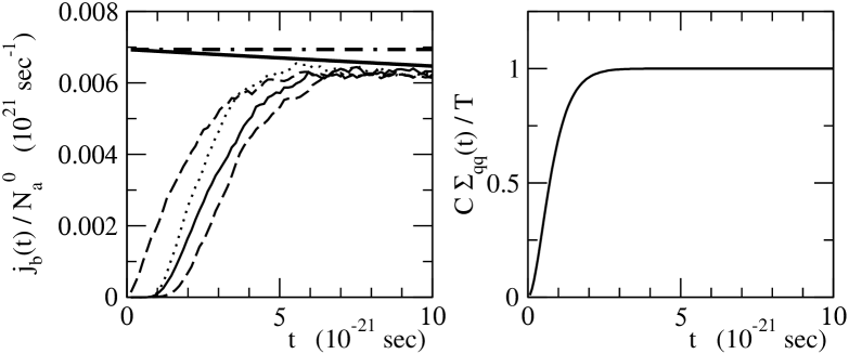
Figure 1: The current across the barrier for different initial distributions, see text.

The figure demonstrates clearly a remarkable uncertainty in the very concept of the ”transient effect”, namely that the $j_{\rm{b}}(t)$ reaches its asymptotic behavior only after some finite time $\tau_{\rm{trans}}$. Even more important appears to be that the whole effect is due to the arbitrariness in choosing time zero. If the calculation were repeated at some later time $t_{0}>\tau_{\rm{trans}}$, the same behavior would be seen! This is due to the fact that the whole transient effect only comes about because in the initial distribution there is some favorable region in phase space from which it is easiest to reach the barrier. This is demonstrated in Fig.2. There, all initial points in phase space are sampled which cross the barrier after some time $\tau_{s}$. On the right a sufficiently large time was chosen such that most parts of the initial distribution have ”fissioned”. As exhibited on the left, for the much shorter time, of the order of $\tau_{\rm{trans}}$, only a small fraction of points have succeeded to do this, namely those which start close to the barrier with a more favorite initial momentum. The vast majority of particles are still waiting to complete the same motion but at a later time! This feature is very important for several reasons, in particular (i) for an understanding of the essentials of the concept of the MFPT [7, 8, 9], (ii) that there still is ample time for neutrons to be emitted inside the barrier, even for $t\gg\tau_{\rm{trans}}$.

Figure 2: Samples of initial points which overcome the saddle within a given time $\tau_{s}$: Left part: $\tau_{s}\simeq\tau_{\rm{trans}}$; right part $\tau_{s}\simeq\tau_{\rm{K}}$.

The calculations have been performed by simulating the Langevin equations exploiting a locally harmonic oscillation, for the following parameters: $T=3$ MeV, $E_{b}=8$ MeV, $\hbar\varpi_{a}=1$ MeV and $\eta_{a}=1$. The potential was constructed from two oscillators, an upright one and one upside down, joined at some point between the minimum and the saddle with a smooth first derivative.

3 The mean first passage time

For the sake of simplicity we take the example of overdamped motion for which the momentum is always in equilibrium such that one only needs to consider the time evolution of the fission coordinate $Q$. The first passage time may then be defined in the following way. Suppose that at $t=0$ the particle starts at the potential minimum $Q_{\rm{a}}$ sharp. Because of the fluctuating force there will be many trajectories $i$ which will pass a certain exit point $Q_{\rm{ex}}$ once. This process may take the time $t_{i}$, the first passage time. The mean-FPT $\tau_{\rm{mfpt}}(Q_{\rm{a}}\to Q_{\rm{ex}})$ is defined by the average $\langle t_{i}\rangle$ over all possibilities. In order to really obtain the mean first passage time the $i$ has to be removed from the ensemble once it has exited the interval at $Q_{\rm{ex}}$: the ”particle” can be said to be absorbed at $Q_{\rm{ex}}$ (”absorbing barrier”). As the potential $V(Q)$ is assumed to rise to infinity for $Q\to-\infty$, any motion to the far left will bounce back: the region $Q\to-\infty$ acts as a ”reflecting barrier”.

The MFPT $\tau_{\rm{mfpt}}$ can also be calculated from solutions $K(Q,t\,|\,Q_{\rm{a}},0)$ of the Smoluchowski equation, adequate for overdamped motion [7, 8, 9]. The initial condition for the particles to start at $Q_{\rm{a}}$ is then: $\lim_{t\to 0}K(Q,t|Q_{\rm{a}},0)=\delta(Q-Q_{\rm{a}})$, which is identical to the one used for the fully drawn line of Fig.1. It is this case which (for constant friction and temperature) allows for an analytic form for the MFPT,

$$\tau_{\rm{mfpt}}(Q_{\rm{a}}\to Q_{\rm{ex}})=\frac{\gamma}{T}\int_{Q_{\rm{a}}}^{Q_{\rm{ex}}}du\;\exp\left[\frac{V(u)}{T}\right]\int_{-\infty}^{u}dv\;\exp\left[-\frac{V(v)}{T}\right]\,,$$ (2)

by reasoning as follows: The probability of finding at time $t$ the particle still inside the interval $(-\infty,~{}Q_{\rm{ex}})$ is given by $W(Q_{\rm{a}},t)=\int_{-\infty}^{Q_{\rm{ex}}}\,dQ\,K(Q,t\,|\,Q_{\rm{a}},0)$. Hence, the probability for it to leave the region during the time lap from $t$ to $t+dt$ is determined by $-dW=-\frac{\partial}{\partial t}W(Q_{\rm{a}},t)dt$, such that one has $\tau_{\rm{mfpt}}(Q_{\rm{a}}\to Q_{\rm{ex}})=-\int tdW$ which turns into

$$\tau_{\rm{mfpt}}(Q_{\rm{a}}\to Q_{\rm{ex}})=\int_{0}^{\infty}\int_{-\infty}^{Q_{\rm{ex}}}\,K(Q,t\,|\,Q_{\rm{a}},0)\,dQ\,dt=\int_{0}^{\infty}dt\,t\,j(Q_{\rm{ex}},t\,|\,Q_{\rm{a}},0)\,.$$ (3)

These formulas are associated to the special boundary conditions with respect to the

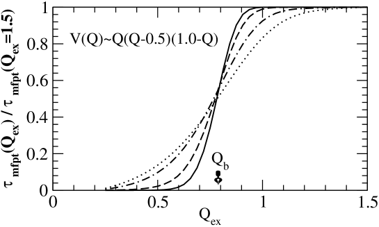
Figure 3: MFPT for the cubic potential normalized to its asymptotic value. Solid, dashed, dotted-dashed and dotted curves correspond to $T/E_{b}=0.1,0.2,0.5,1.0$.

coordinate mentioned before, the reflecting barrier at $Q\to-\infty$ and an absorbing barrier at $Q_{\rm{ex}}$. In particular for the latter reason it is not permitted to use in (3) the currents shown in Fig.1. Inserting them blindly would indeed lead to expressions for $\tau_{\rm{mfpt}}$ in which the $\tau_{\rm{trans}}$ appears. This is in clear distinction to the correct expression (2). Actually, the derivation of (2) involves proper solutions of that equation which is ”adjoint” to the Smoluchowski equation, and which describes motion backward in time. In Fig.3 we show the dependence of $\tau_{\rm{mfpt}}(Q_{\rm{a}}\to Q_{\rm{ex}})$ on $Q_{\rm{ex}}$ as given by (2) calculated for a cubic potential. Evidently, the MFPT needed to reach the saddle at $Q_{\rm{b}}$ is exactly half the asymptotic value. The latter may be identified as the mean fission life time $\tau_{f}\equiv\tau_{\rm{mfpt}}(Q_{\rm{a}}\to Q_{\rm{ex}}\gg Q_{\rm{b}})$. For the typical conditions under which Kramers’ rate formula (1) is valid for overdamped motion, this relation of $R_{\rm{K}}=\left(\tau_{f}\right)^{-1}$ to the asymptotic MFPT can be derived analytically [8]. Another remarkable feature seen in Fig.3 is the insensitivity of the MFPT to the exit point for small and large $Q_{\rm{ex}}$.

4 Discussion

It should be evident from the previous discussion that in the very concept of the MFPT there is no room for a transient effect. After all, formula (2) is based on exact solutions of the transport equation which satisfy the same initial condition as those used for the plots in Fig.1. One essential difference is seen in the fact that the evaluation of the MFPT takes into account an average over all initial points, as is warranted by the definition of the MFPT through the probability distribution $-dW$. Contrasting this feature, and as outlined in sect.2, the transient effect only represents a minor part of the initial population, namely that one which reaches the barrier first. Discarding the rest implies ignoring the many particles which are still moving inside the barrier for times typically much longer than $\tau_{\rm{mfpt}}(Q_{\rm{a}}\to Q_{\rm{b}})$. Neutrons from deformations corresponding to that region are not only emitted within $\tau_{\rm{trans}}$ but within $\tau_{\rm{mfpt}}(Q_{\rm{a}}\to Q_{\rm{b}})$, which turns out to be just half of the total fission time $\tau_{\rm{K}}$. Of course, this discussion shows that — besides the additional neutrons often associated to the transient effect — also those, supposedly emitted during the motion from saddle to scission are not treated correctly by introducing the saddle to scission time $\tau_{\rm{ssc}}$ of [10]. As one may guess from Fig.3, like the $\tau_{\rm{trans}}$, the $\tau_{\rm{ssc}}$ does not appear to be in accord with the MFPT either. These findings suggest that one simply estimates the emission rate of neutrons over fission from the ratio $\Gamma_{n}/\Gamma_{\rm{K}}$. Anything else does not seem to be in accord with the assumption that fission can be described by the Kramers or Smoluchowski equations, for the usually assumed form of the potential. This does not rule out any effects related to a more complicated dynamics, in particular if the initial stage of the whole reaction is to be described with a different transport theory. These findings may perhaps imply that some of the existing statistical codes will have to be revised. The question of the temperature dependence of nuclear transport does not seem to be a closed one yet. A theoretical prediction has been given in [3].

The authors benefitted greatly from a collaboration meeting on ”Fission at finite thermal excitations” in April, 2002, sponsored by the ECT* (’STATE’ contract). One of us (F.A.I.) would like to thank the Physik Department of the TUM for the hospitality extended to him during his stay at Garching.

References

- [1] P. Paul and M. Thoennessen, Ann. Rev. Part. Nucl. Sci. 44 (1994) 65
- [2] H.A. Kramers, Physica 7 (1940) 284
- [3] H. Hofmann, F.A. Ivanyuk, C. Rummel and S. Yamaji, Phys. Rev.C, 64 (2001) 054316
- [4] P. Grangé, J.-L. Li and H.A. Weidenmüller, Phys. Rev. C27 (1983) 2063
- [5] K. H. Bhatt, P. Grangé and B. Hiller, Phys. Rev. C33 (1986) 954
- [6] K.Pomorski, J.Bartel, J.Richert and K. Dietrich, Nucl. Phys. A605 (1996) 87; P.Fröbrich and I.I.Gontchar, Phys.Rep. 292 (1998) 131; Y.Aritomo, T.Wada, M.Ohta and Y.Abe, Phys. Rev. C 55 (1997) 1011
- [7] N.G. van Kampen: ”Stochastic processes in physics and chemistry ”, North-Holland, 2001, Amsterdam
- [8] C.W. Gardiner, ”Handbook of stochastic methods, Springer, 2002, Berlin
- [9] H. Risken, ”The Fokker-Planck-Equation”, Springer, Berlin, 1989
- [10] H. Hofmann and J.R. Nix, Phys. Lett.B 122 (1983) 117