PHOTON EXCHANGE IN NUCLEUS-NUCLEUS COLLISIONS

Abstract

The strong electromagnetic fields in peripheral heavy ion collisions give rise to photon-photon and photon-nucleus interactions. I present a general survey of the photon-photon and photon-hadron physics accessible in these collisions. Among these processes I discuss the nuclear fragmentation through the excitation of giant resonances, the Coulomb dissociation method for application in nuclear astrophysics, and the production of particles.

1 Peripheral Heavy Ion Collisions

The field of peripheral atomic collisions was born in 1924, when E. Fermi had the ingenious idea of relating the atomic processes induced by fast charged particles to processes induced by electromagnetic waves. In 1934-1935, Weizsäcker and Williams modified Fermi’s calculation by including the appropriate relativistic corrections. The original Fermi’s idea is now known as the Weizsäcker-Williams method [2, 3], an approximation widely used in coherent processes in atomic, nuclear and particle physics. In Fermi’s method the electromagnetic (strong) field generated by a fast particle is replaced by a flux of equivalent photons (flux mesons or gluons).

In peripheral heavy ion collisions (PHIC) the number of equivalent photons, $n(\omega)$ of energy $\omega$ can be calculated classically, or quantum-mechanically. For the electric dipole (E1) multipolarity both results are identical under the assumption of very forward scattering [4]. In ref. [4] the number of equivalent photons for all multipolarities was calculated exactly. It was shown that for the electric dipole multipolarity, E1, the equivalent photon number, $n_{E1}(\omega)$, coincides with the one deduced by Weizsäcker and Williams. It was also shown that in the extreme relativistic collisions the equivalent photon numbers for all multipolarities agree, i.e, $n_{E1}(\omega)\sim n_{E2}(\omega)\sim n_{M1}(\omega)\sim...$. This is shown in figure 1.

According to Fermi’s idea, the cross sections for one- and two-photon processes depicted in figure 2(a,b) are given by

$$\sigma_{X}=\int d\omega\frac{n\left(\omega\right)}{\omega}\sigma_{X}^{\gamma}\left(\omega\right)\;,\;{\rm and}\;\;\sigma_{X}=\int d\omega_{1}d\omega_{2}\frac{n\left(\omega_{1}\right)}{\omega_{1}}\frac{n\left(\omega_{2}\right)}{\omega_{2}}\sigma_{X}^{\gamma\gamma}\left(\omega_{1},\omega_{2}\right)\;,$$ (1)

where $\sigma_{X}^{\gamma}\left(\omega\right)$ is the photon-induced cross section for the energy $\omega$, and $\sigma_{X}^{\gamma\gamma}\left(\omega_{1},\omega_{2}\right)$ is the two-photon cross section. Note that we do not refer to the photon momenta. The virtual photons are real: $q^{2}=0$, a relation always valid for PHIC.

Figure 1: Virtual photon numbers (in units of $Z^{2}\alpha$) for the E1, E2 and M1 multipolarities. Upper (lower) figure is for $\gamma=2$ ($\gamma=100$). $\omega$ is the photon energy and $R$ is the sum of the nuclear radii.

At relativistic bombarding energies one has (in natural units)

$$n(\omega)={2\over\pi}Z_{p}^{2}\alpha\ln\left({\gamma\over\omega R}\right)\ ,$$ (2)

where $\gamma=(1-v^{2})^{-1/2}$ is the relativistic Lorentz factor in the frame of reference of the target, $Z_{p}e$ is the projectile charge and $\alpha=1/137$.

Eq. 1 is called the equivalent photon approximation (EPA), or Weizsäcker-Williams method. It is valid for processes c, d, e, and f in figure 2. But the approximation is not applicable to processes a and b in figure 2, in which multiple virtual photons are exchanged between the projectile, the target, and/or with the produced particle(s).

For one-photon processes, e.g., Coulomb fragmentation, $\sigma_{X}^{\gamma}\left(\omega\right)$ is localized in a small energy interval and one gets a cross section in the form $\sigma=A\ln\gamma+B$, where $A$ and $B$ are coefficients depending on the system. The $\ln\gamma$ factor is due to the equivalent photon number, $n\left(\omega\right)$, which is approximately independent of $\omega$ in the integral range of interest. For two-photon processes, besides the $\ln^{2}\gamma_{c}$ from $n_{1}$ and $n_{2}$, a third $\ln\gamma_{c}$ arises from the integral over $\omega_{1}$ ($\omega_{1}$ and $\omega_{2}$ are related by energy conservation). Note that here we used $\gamma_{c}$ of a heavy ion collider, so that $\gamma=2\gamma_{c}^{2}-1$, with $\gamma_{c}$ the collider Lorentz gamma factor (e.g., $\gamma_{c}\sim 100$ for the RHIC collider at Brookhaven).

Most applications of PHIC were reviewed in ref. [5]. Since then a great amount of work has been performed in this field. The coherent $\gamma$-$\gamma$ and $\gamma$-A interactions in very peripheral collisions at relativistic ion colliders has been reviewed recently in ref. [6]. In this review article I will present a general account of the theory and the latest developments in the field of PHIC with fixed targets at intermediate energies ($E_{Lab}\simeq 100$ MeV/nucleon), and at ultra-relativistic energies of present day (the Relativistic Heavy Ion Collider (RHIC), at Brookhaven) and future heavy ion collider (the Large Hadron Collider (LHC), at CERN) energies .

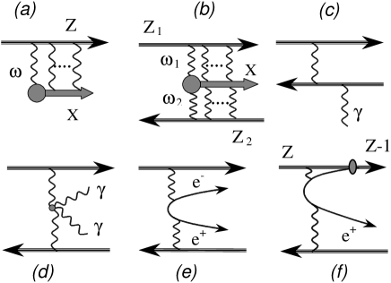
Figure 2: PHIC processes: (a) one-photon, (b) two-photon, (c) Bremsstrahlung, (d) Delbrück scattering, (e) pair-production, and (f) pair-production with capture.

2 Relativistic Coulomb Excitation and Fragmentation

Relativistic Coulomb excitation is now a popular tool for the investigation of the intrinsic nuclear dynamics and structure of the colliding nuclei, specially important in reactions involving radioactive nuclear beams [1, 7, 8, 9, 10, 11, 12]. The advantage is that the Coulomb interaction is very well known. The disadvantage is that the contribution of the nuclear-induced processes also play a role in some situations. The treatment of the dissociation problem by nuclear forces is very model dependent, based on eikonal or multiple Glauber scattering approaches [7, 13, 14, 15, 16]. Among the uncertainties are the in-medium nucleon-nucleon cross sections, the multiple scattering process and the separation of stripping from elastic dissociation of the nuclei [16]. Nonetheless, specially for the very weakly-bound nuclei, relativistic Coulomb excitation has lead to very exciting new results [7, 8, 13, 14, 15].

2.1 Reactions with Radioactive Beams

Coulomb breakup of weakly-bound nuclei may involve single or multiple photon-exchange between the projectile and the target. In the first case, perturbation theory gives a direct relation between the data and the matrix elements of electromagnetic transitions. Such matrix elements are the clearest probes of the nuclear structure of these nuclei, since one cannot perform experiments with real photons or with electron scattering off nuclei far from the stability valley. In the second case, often called by post-acceleration, or reacceleration, effects [13, 14, 15, 17, 18], one has to perform a non-perturbative treatment of the reaction what complicates the extraction of the electromagnetic (mainly E1) matrix elements.

Among several possible studies of interest, one expects to learn if the Coulomb-induced breakup proceeds via a resonance or by the direct dissociation into continuum states [13, 14, 15]. There is a strong ongoing effort to use the relativistic Coulomb excitation technique also for studying bound excited states in exotic nuclei, to obtain information on gamma-decay widths, angular momentum, parity, and other properties of hitherto unknown states [8, 11, 12].

Figure 3: S-factors ($S_{17}$) for the ${}^{7}Be(p,\gamma)^{8}B$ reaction. The inset is a blowup of the low energy region. See text for details.

Another application of peripheral collisions with radioactive nuclear beams is in astrophysics. Radiative capture reactions are known to play a major role in astrophysical sites, e.g., in a pre-supernova [19, 20]. Some reactions of interest for astrophysics, e.g., ${}^{7}Be\left(p,\gamma\right)^{8}B$, can be studied via the inverse photo-dissociation reaction ${}^{8}B\left(\gamma,p\right)^{7}Be$ [21]. Since the equivalent photon numbers in eq. 1 can be calculated theoretically , an experimental measurement of the Coulomb breakup reaction $a+A\longrightarrow b+c+A$ is useful to obtain the corresponding $\gamma$ induced cross section $\gamma+a\longrightarrow b+c$. Using detailed balance, this cross section can be related to the radiative capture cross section $b+c\longrightarrow a+\gamma,$ of astrophysical interest [21] (see eq. 4).

The radiative capture cross sections in nuclear astrophysics are often written in terms of the astrophysical S-factor [19, 20], defined by

$$S(E)=E\sigma\left(E\right)\exp\left[2\pi\eta\left(E\right)\right]\ ,$$ (3)

where $\eta\left(E\right)=Z_{b}Z_{c}e^{2}/\hbar\sqrt{2\mu_{bc}E}$, and $E$ is the relative kinetic energy of the nuclei $b$ and $c$ in the reaction $b(c,\gamma)a$. The cross section for the dissociation process $a+A\longrightarrow b+c+A$ can be written as

$${d\sigma\over dE}={\mu_{bc}c^{2}\over E_{x}^{3}}\ n(E_{x})\ {(2J_{b}+1)(2J_{c}+1)\over(2J_{a}+1)}\ S(E)\ \exp\left[-2\pi\eta\left(E\right)\right]\ ,$$ (4)

where $E_{x}=E+B$ is the sum of the relative energy $E$ and the binding energy $B$ of the two fragments. $J_{i}$ is the ground-state angular momentum of the nucleus i.

Table 1: Radiative capture reactions of interest in nuclear astrophysics which can be studied with the Coulomb dissociation method.

Reaction	$T_{1/2}$ (projectile)	Astrophysical application
${}^{3}He\left(\alpha,\gamma\right)^{7}Be$	53.3 days	Solar-neutrinos
${}^{7}Be\left(p,\gamma\right)^{8}B$	770 ms	${}^{3}He$ abundance
${}^{7}Be\left(\alpha,\gamma\right)^{11}C$	20.4 min
${}^{4}He\left(d,\gamma\right)^{6}Li$	Stable	Primordial nucleosynthesis
${}^{6}Li\left(p,\gamma\right)^{7}Be$	53.3 days
${}^{6}Li\left(\alpha,\gamma\right)^{10}B$	Stable
${}^{4}He\left(t,\gamma\right)^{7}Li$	Stable
${}^{7}Li\left(\alpha,\gamma\right)^{11}B$	Stable
${}^{11}B\left(p,\gamma\right)^{12}C$	Stable
${}^{9}Be\left(p,\gamma\right)^{10}B$	Stable
${}^{10}B\left(p,\gamma\right)^{11}C$	20.4 min
${}^{7}Li\left(n,\gamma\right)^{8}Li$	842 ms	Inhomogeneous Big Bang
${}^{8}Li\left(n,\gamma\right)^{9}Li$	178 ms
${}^{12}C\left(n,\gamma\right)^{13}C$	Stable
${}^{14}C\left(n,\gamma\right)^{15}C$	2.45 s
${}^{14}C\left(\alpha,\gamma\right)^{18}O$	Stable
${}^{12}C\left(p,\gamma\right)^{13}N$	10 min	CNO cycles
${}^{16}O\left(p,\gamma\right)^{17}F$	65 s
${}^{13}N\left(p,\gamma\right)^{14}O$	70.6 s
${}^{20}Ne\left(p,\gamma\right)^{21}Na$	22.5 s
${}^{11}C\left(p,\gamma\right)^{12}N$	11 ms	Hot p-p chain
${}^{15}O\left(\alpha,\gamma\right)^{19}Ne$	17.2 s	rp process
${}^{31}S\left(p,\gamma\right)^{32}Cl$	291 ms
${}^{12}C\left(\alpha,\gamma\right)^{16}O$	Stable	Helium burning
${}^{16}O\left(\alpha,\gamma\right)^{20}Ne$	Stable
${}^{14}N\left(\alpha,\gamma\right)^{18}F$	109.7 min
${}^{22}Mg\left(p,\gamma\right)^{23}Al$	3.86 s	rp bottlenecks

The Coulomb dissociation method is more useful when higher order effects are under control, so that the eq. 4, obtained in 1st-order perturbation theory, is valid. Higher order effects can be taken into account in a coupled channels approach, or by using higher order perturbation theory.

Expanding the nuclear wave function in the set $\{\mid j\rangle;\ j=1,N\}$ of eigenstates of the intrinsic Hamiltonian $H_{0}$, where $N$ is the number states included in the calculation, one obtains the coupled equations for the occupation amplitude of the state $k$ as

$$i\hbar\ {\dot{a}}_{k}(t)=\sum_{j=1}^{N}\ \langle k\mid V(t)\mid j\rangle\;\exp\left[i(E_{k}-E_{j})t/\hbar\right]\;a_{j}(t)\;,\qquad\qquad k=1\;\mathrm{to}\;\;N\ ,$$ (5)

where $E_{n}$ is the energy of the state $\left|n\right\rangle.$ This set of equations can be solved numerically if one has a theoretical model or experimental information on the matrix elements $\langle k\mid V(t)\mid j\rangle$. In the most relevant situations the perturbing potential is the Coulomb interaction of the fragments with the target. This interaction is expanded into electric and magnetic multipolarities. One thus needs information on the electromagnetic matrix elements between the bound states and the continuum states of the nucleus to carry out the coupled-channels calculation. This approach has been used in refs. [22, 23] to treat the problem of Coulomb reacceleration of fragments following the breakup. More recently, a similar technique has been used in ref. [24].

Another approach to the Coulomb postacceleration, or reacceleration, problem is to integrate the time-dependent Schrödinger equation directly for a given model Hamiltonian. This approach is only useful when one can use a two-body potential model for the nucleus. Then, expanding the two-body wavefunction into angular components one gets the time-dependent wave equation

$$\left[{d^{2}\over dr^{2}}-{l(l+1)\over r^{2}}-{2\mu_{bc}\over\hbar}V(r)\right]u_{lm}(r)+\sum_{l^{\prime}m^{\prime}}S_{l^{\prime}m^{\prime}}^{lm}u_{l^{\prime}m^{\prime}}(r)=-{2\mu_{bc}\over\hbar}{\partial u_{lm}\over\partial t}$$ (6)

where $u_{lm}(r)$ is the radial part of the $lm$-component of the two-body wavefunction. $S_{l^{\prime}m^{\prime}}^{lm}$ is a source term for the postacceleration, arising from the multipole component $lm$ of the Coulomb field of the target. This approach has been used in ref. [15] and later developed in refs. [17, 18, 25, 26, 27].

As an example of application of the Coulomb dissociation method, we show in figure 3 the result of an experiment performed at the GSI laboratory, in Darmstadt, Germany [28]. The S-factor obtained in this experiment is shown in figure 3 as solid circles, by a direct application of eq. 4, using $S_{17}(E)$ obtained from theoretical models. The solid curve is a fit using a theoretical model of ref. [23], whereas the dashed curve is a calculation done in ref. [29].

Alternative experiments have obtained $S_{17}$ by measuring the parallel momentum distribution of the fragments after Coulomb breakup [33, 32]. This technique was applied to several experiments at the NSCL laboratory, of Michigan State University [32, 31, 30]. The technique also allows the disentanglement of the E1 and E2 contributions to the breakup by looking at the asymmetries in the momentum distribution following the Coulomb breakup of the projectile [33].

In table I a set of reactions are shown which can be studied with the Coulomb dissociation method [34].

Besides the reaction ${}^{7}Be\left(p,\gamma\right)^{8}B$, the Coulomb dissociation method has also been applied to the study of ${}^{4}He\left(d,\gamma\right)^{6}Li$ (see ref. [35]), ${}^{12}C\left(n,\gamma\right)^{13}C$ (see ref. [36, 37]), ${}^{11}C\left(p,\gamma\right)^{12}N$ (see ref. [38]), and ${}^{12}C\left(\alpha,\gamma\right)^{16}O$ (see ref. [39]).

2.2 Multiphonon Resonances

Giant dipole resonances (GDR) occur in nuclei at energies around 10-20 MeV. Assuming that they are harmonic vibrations of protons against neutrons, one expects that DGDRs (Double Giant Dipole Resonances), i.e., two giant dipole vibrations superimposed in one nucleus, will have exactly twice the energy of the GDR [5, 9, 10].

Assuming that one knows $\sigma^{GDR}_{\gamma}(E)$ somehow (either from experiments, or from theory), a simple harmonic model can be formulated to obtain the Coulomb excitation cross sections of these states. In this model the inclusion of the coupling between all multiphonon states can be performed analytically [40]. Following the same reasoning leading to eq. 1, to first-order the probability to excite a giant resonance state at energy $E$ is given by

$$P^{1st}(E,b)={N(E,b)\over E}\ \sigma^{GDR}_{\gamma}(E)\ ,$$ (7)

where $N(E,b)$ is the number of equivalent photons per unit area in a collision at impact parameter $b$. The relation between $n(E)$ of eq. 1 and $N(E,b)$ is given by $n(E)=2\pi\int N(E,b)\ b\ db$.

In the harmonic oscillator model the excitation probabilities calculated to first-order, are modified to include the flux of probability to the other states [5]. That is,

$$P(E,\;b)=P^{1st}(E,b)\;\exp\left\{-P^{1st}(b)\right\}\;,$$ (8)

where $P^{1st}(b)$ is the integral of $P(E,b)$ over the excitation energy $E$. In general, the probability to reach a multiphonon state with the energy $E^{(n)}$ from the ground state, with energy $E^{(0)},$ is obtained by an integral over all intermediate energies [41]

$$P^{(n)}(E^{(n)},b)=\frac{1}{n!}\;\exp\left\{-P^{1st}(b)\right\}\int dE^{(n-1)}\;dE^{(n-2)}\;...\;dE^{(1)}$$ (9)

$$\times P^{1st}(E^{(n)}-E^{(n-1)},b)\;P^{1st}(E^{(n-1)}-E^{(n-2)},b)\;...\;P^{1st}(E^{(1)}-E^{(0)},b)\ .$$ (10)

Integrating this equation over impact parameters yields the cross section for the excitation of the multiphonon state $n$, as a function of the excitation energy $E^{(n)}$.

A series of experiments at the GSI laboratory have obtained the energy spectra, cross sections, and angular distribution of fragments following the decay of the DGDR [42, 43, 44, 45, 46, 47, 48]. It was shown that the experimental cross sections are about 30% bigger than the theoretical ones. This is shown in figure 4 where the cross sections for the excitation of 1-phonon (GDR),

$$\sigma_{1}\sim 2\pi S\ln\left[{2\gamma A_{T}^{1/3}\over A_{P}^{1/3}+A_{T}^{1/3}}\right]\ ,$$ (11)

while for the 2-phonon state it is

$$\sigma\sim 0.1\ {S^{2}\over\left(A_{P}^{1/3}+A_{T}^{1/3}\right)^{2}\ {\rm mb}}\ ,$$ (12)

where

$$S=5.45\times 10^{-4}{Z_{P}^{2}Z_{T}N_{T}\over A_{T}^{2/3}}\ \ \ {\rm mb}\ .$$ (13)

The dashed lines of figure 4 are the result of more elaborate calculations [9, 10, 49, 50, 51, 52, 53].

The GSI experiments are very promising for the studies of the nuclear response in very collective states. One should notice that after many years of study of the GDRs and other collective modes, the width of these states are still poorly explained theoretically, even with the best microscopic approaches known sofar. The extension of these approaches to the study of the width of the DGDRs will be helpful to improve such models [10].

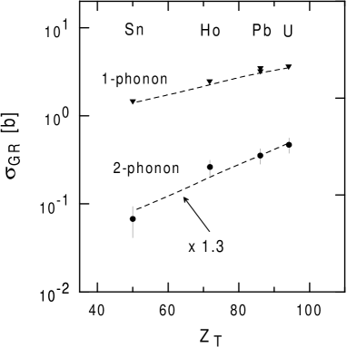
Figure 4: Cross sections for the excitation of the GDR and the DGDR for several systems. The dashed curves are theoretical calculations. See text for more details.

In heavy ion colliders the mutual Coulomb excitation of the ions (leading to their simultaneous fragmentation) is a useful tool for beam monitoring [54]. A recent measurement at RHIC [55], using the Zero Degree Calorimeter to measure the neutron decay of the reaction products, has proved the feasibility of the method. The theoretical prediction of about 3 b for this process, agrees quite well with the experimental results.

The DGDR contributes to only about 10% of the total fragmentation cross section induced by Coulomb excitation in PHIC. The main contribution arises from the excitation of a single GDR, which decays mostly by neutron emission. This is also a potential source of beam loss in relativistic heavy ion colliders [1], and an important fragmentation mode of relativistic nuclei in cosmic rays.

3 Atomic Processes

3.1 Atomic ionization

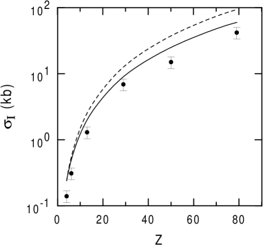
Figure 5: Atomic ionization cross sections for $Pb^{81+}$ (33 TeV) projectiles impinging on several targets. The solid and dashed curves are theoretical calculations. See text for more details.

The cross sections for atomic ionization in PHIC are very large, of order of kilobarns, increasing slowly with the logarithm of the RHI energy. For a fixed target experiment using naked projectiles one gets [5] (here we use $\hbar=c=1$)

$$\sigma_{I}=\zeta(3)\ {Z_{P}^{2}r_{e}^{2}\over\left(Z_{T}\alpha\right)^{2}}\left[1.8\pi+9.8\ln\left({2\gamma\over Z_{T}\alpha}\right)\right]$$ (14)

which decreases with the target charge $Z_{T}$. This is due to the increase of the binding energy of $K$-electrons with the atomic charge. The probability to eject a $K$-electron is much larger than for other atomic orbitals. In this equation $r_{e}=e^{2}/m$ is the classical electron radius, and $\zeta(3)=1.202$ accounts for the ionization of electrons from higher orbits.

The first term inside brackets in eq. 14 is due to close collisions assuming elastic scattering of the electron off the projectile, while the second part is for distant collisions, with impact parameter larger than the Bohr radius [5]. Recently, Baltz [56] has shown that the numerical factors in the equation above should be replaced by $1.8\rightarrow 1.74-1.83$ and $9.8\rightarrow 7.21$, respectively, when one treats the electronic wavefunctions with the relativistic corrections.

Recent experiments have reported ionization cross sections for $Pb^{81+}$ (33 TeV) beams on several targets [57]. In this case, the role of projectile and target are exchanged in the previous equation. In figure 5 show the results of eq. 14 (dashed line) are compared to the experimental data. Since the targets are screened by their electrons, the discrepancy is expected. Calculations by Anholt, Becker and collaborators [58, 59, 60] (solid line) or of Baltz [56] also yield larger cross sections than the experimental data.

Non-perturbative calculations, solving the time dependent Dirac equation exactly, were first performed by Giessen and Oak Ridge groups [61, 62]. The main problem is to adequately treat the several channels competing with the ionization process, specially for atoms with more than one electron. Also, the effects of screening (static and dynamic) are hard to calculate. On the experimental side, there are little data available for a meaningful comparison with theory. However, atomic ionization should be taken seriously in accelerator design when a residual gas remains in the accelerator pipes.

3.2 Bremsstrahlung and Delbrück scattering

Bremsstrahlung (fig. 2c) is a minor effect in PHIC. It has been calculated in ref. [5, 63]. The cross section is proportional to the inverse of the square mass of the ions. Most virtual photons have very low energies. For 10 MeV photons the central collisions deliver 10⁶ more photons than the peripheral ones [63].

For a collider the Bremsstrahlung differential cross section is given by

$${d\sigma_{\gamma}\over d\omega}={16Z^{6}\alpha^{3}\over 3\omega A^{2}m_{N}^{2}}\ln\left({\gamma\over\omega R}\right)\ ,$$ (15)

where $m_{N}$ is the nucleon mass, $\gamma=2\gamma_{c}^{2}-1$, where $\gamma_{c}$ is the collider Lorentz gamma factor ($\gamma_{c}\sim 100$ for RHIC/BNL), and $R$ is the nuclear dimension ($R\sim 2.4\times A^{1/3}$ fm) [63].

For very low energy photons ($\omega\sim 100$ eV) the whole set of particles in a beam bunch can act coherently and a great number of Bremsstrahlung photons can be produced. This has been proposed as a tool for monitoring the bunch dimension in colliders [64]. Recently, an experiment has been approved at RHIC/BNL to measure this kind of coherent effect, including the emission of real photons by the interaction of a bunch with the edges of the accelerator magnets [65].

Delbruck scattering ($\gamma^{\ast}+\gamma^{\ast}\longrightarrow\gamma+\gamma$) involves an additional $\alpha^{2}$ as compared to pair production and has never been possible to study experimentally.  The cross section is about 50 b for the LHC [63] and the process is dominated by high-energy photons, $E_{\gamma}\gg m_{e}$. A study of this process in PHIC is thus promising if the background problems arising from central collisions can be eliminated. No experiments of Bremsstrahlung or Delbrück scattering in PHIC have been performed so far. The total cross section for Delbrück scattering ($\omega\gg m_{e}$) in colliders is given by [63]

$$\sigma=2.54Z^{4}\alpha^{4}r_{e}^{2}\ln^{3}\left({\gamma\over m_{e}R}\right)\ .$$ (16)

4 The Electromagnetic Field of an Ultrarelativistic Charge

As discussed above, the calculation of processes involving the multiple exchange of photons is not as easy to perform. For example, substantial differences have been found between the cross sections for the production of $e^{+}e^{-}$ pairs calculated within several approaches [67, 68]. However, the calculation of multiple photon exchange can be considerably simplified at very high bombarding energies if one assumes that the electromagnetic field generated by the projectile (or target, depending on the reference frame) lies entirely on a plane perpendicular to its trajectory [69]. We show next that this approximation is well justified [70].

The scalar part of the electromagnetic potential generated by an ultrarelativistic particle is proportional to $V\left(\mbox{\boldmath$\rho$},z,t\right)=\phi\left(\mbox{ \boldmath$\rho$},z,t\right)$ where $\phi\left(\mbox{\boldmath$\rho$},z,t\right)$ is the Lienard-Wiechert potential at a point ${\bf r}=\left(\mbox{\boldmath$\rho$},z\right)$, generated by a relativistic particle with velocity ${\bf v}=v\hat{\bf z}$ and impact parameter ${\bf b}$ (in our units $\hbar=c=m_{e}=1$),

$$\phi\left(\mbox{\boldmath$\rho$},z,t\right)=\gamma Z\alpha\left[\left({\bf b}-\mbox{\boldmath$\rho$}\right)^{2}+\gamma^{2}\left(z-vt\right)^{2}\right]^{-1/2}\;.$$ (17)

In these expressions $\gamma=\left(1-v^{2}\right)^{-1/2}$ is the Lorentz contraction factor. The vector part of the electromagnetic interaction is proportional to eq. 17 and , for simplicity, we leave it out of this proof.

Using the Bethe-integral [5], the potential (17) can be written in the form

$$\phi\left(\mbox{\boldmath$\rho$},z,t\right)=Z\alpha\,\frac{1}{2\pi^{2}}\int d^{3}q\frac{e^{-i{\bf q.u}}e^{i{\bf q.r}}}{q^{2}-v^{2}q^{2}_{z}}\,,$$ (18)

where ${\bf u}={\bf b}+{\bf v}t$ and $q=\left({\bf q}_{t},\ q_{z}\right)$. The integral in (18) diverges logarithmically as $v\,\rightarrow\,1$.

For practical purposes one needs the interaction in the form $V\left(\mbox{\boldmath$\rho$},z,t\right)=\phi\left(\mbox{\boldmath$\rho$},z,t\right)-\phi\left(0,z,t\right)$, i.e.,

$$V\left(\mbox{\boldmath$\rho$},z,t\right)=Z\alpha\,\,\frac{1}{2\pi^{2}}\int d^{3}q\ e^{-i{\bf{\bf q.u}}}\frac{\left[e^{i{\bf q.r}}-e^{iq_{z}z}\right]}{q_{t}^{2}+q^{2}_{z}/\gamma^{2}}\,.$$ (19)

Let us define

$$\Phi\left(\mbox{\boldmath$\rho$},z,t\right) \equiv {V\left(\mbox{\boldmath$\rho$},z,t\right)\over Z\alpha\,}$$ (20)

$$= \frac{1}{\pi}\int d^{2}q_{t}\,\frac{1}{q^{2}_{t}}\,\exp{(-i{\bf q}_{t}.{\bf b})}\,\left[\exp{(i{\bf q}_{t}.\mbox{\boldmath$\rho$})}-1\right]\,\Phi_{z}\left({\bf q}_{t},z,t\right)\,.$$

Then

$$\Phi_{z}\left({\bf q}_{t},z,t\right)=\frac{q^{2}_{t}}{2\pi}\int dq_{z}\frac{e^{iq_{z}\left(z-vt\right)}}{q_{t}^{2}+q^{2}_{z}/\gamma^{2}}=\frac{\gamma q_{t}}{2}e^{-\gamma q_{t}|z-vt|}\,.$$ (21)

Now, using $\lim_{\Lambda\rightarrow\infty}\,\left(\Lambda/2\right)e^{-\Lambda|x|}=\delta\left(x\right)$, we see that for $\gamma\rightarrow\infty$, $\Phi_{z}$ does not depend on $q_{t}$, and assumes the form of a delta function: $\Phi_{z}\left(z,t\right)=\delta\left(z-vt\right)$.

In this limit, we can write (20) as

$$\Phi\left(\mbox{\boldmath$\rho$},z,t\right)=\delta\left(z-t\right)\Phi_{\rho}\left(\mbox{\boldmath$\rho$},t\right)\,,$$ (22)

with

$$\Phi_{\rho}\left(\mbox{\boldmath$\rho$},t\right) = \frac{1}{\pi}\int d^{2}q_{t}\,\frac{1}{q^{2}_{t}}\,\exp{(-i{\bf q}_{t}.{\bf b})}\,\left[\exp{(i{\bf q}_{t}.\mbox{\boldmath$\rho$})}-1\right]$$ (23)

$$= 2\int\frac{dq_{t}}{q_{t}}\left\{J_{0}\left[q_{t}|\mbox{\boldmath$\rho$}-b|\right]-J_{0}\left(q_{t}b\right)\right\}\,,$$

where $J_{0}$ is the cylindrical Bessel function. The integral over each Bessel function diverges, but their difference does not. To show this one regularizes the integrals by using

$$\int dx\,\frac{xJ_{0}\left(ax\right)}{x^{2}+k^{2}}=K_{0}\left(ak\right)\,,$$ (24)

where $K_{0}$ is the modified cylindrical Bessel function. Taking the limit $k\rightarrow 0$, and using $K\left(ak\right)\simeq\ln\left(ak\right)$, for small values of $ak$, one gets

$$\Phi\left(\mbox{\boldmath$\rho$},t\right)=\ln\frac{\left({\bf b}-\mbox{\boldmath$\rho$}\right)^{2}}{b^{2}}\,.$$ (25)

This is the solution of the Coulomb potential of a unit charge in 2-dimensions. An easy way to see this is to use Gauss law for the electric field in two dimensions. One obtains $E\simeq 1/b$, where $b$ is the distance to the charge. Since $E=-\partial\Phi/\partial b$, the logarithmic form of $\Phi$ is evident.

The above derivation illustrates the validity of the approximation in terms of the transverse momentum transfer $q_{t}$. It should fail for very soft processes, i.e., those for which $q_{t}$$\rightarrow 0.$ Also, it requires that $q_{z}$ is small compared to $\gamma$. As shown in ref. [5], $q_{z}$ values up to $\gamma$ units of the electron mass contribute appreciably to the integrals involved in the production of free, and of bound-free, $e^{+}e^{-}$ pairs.

The delta-function interaction yields reasonable results as long as $\omega b/\gamma\leq 0.1.$ [70]. This amounts to $b\leq 0.1\gamma/\omega$. As shown in ref. [5], the most effective impact parameters for this process are of the order of  $b\simeq 1/m$. In ref. [70] it has been shown that the differential cross sections for $e^{+}e^{-}$ pair production are well described up to energies of the order of $0.1\gamma m$, by using the delta-function interaction.

For other situations, e.g., nuclear fragmentation due to the electromagnetic interaction, the most effective impact parameter is given by $b\simeq R$, where $R\simeq 10$ fm. We thus expect that the delta-function interaction works well for $\varepsilon\leq 0.1\gamma$ MeV. Note that $\gamma$ is huge for RHIC and LHC energies, and the approximation works well for all energies of practical interest in nuclear fragmentation.

The basic idea of the delta-function interaction is that the electromagnetic field of a relativistic charge looks like a very thin pancake. Those processes which do not involve too large energy transfers, will not be sensitive to the spatial variation of the field. Then the delta-function is a good approximation. For typical energy transfers of the order of 10-100 MeV in nuclear fragmentation, the approximation works well for $b\leq 0.1\gamma/\omega$ fm. To calculate total cross sections it is always necessary to account for those large impact parameters at which the delta-function approximation fails. Similar conclusions have been drawn in a recent article on projectile-electron loss in relativistic collisions with atomic targets [71].

4.1 Free and bound-free electron-positron pair production

It has been demonstrated long time ago [72, 73, 74, 75] that to leading order in $\ln\gamma$, the $e^{+}e^{-}$-pair production in PHIC is given by

$$\sigma={28\over 27\pi}\ Z_{P}^{2}Z_{T}^{2}r_{e}^{2}\ln^{3}\left({\gamma\over 4}\right)\ .$$ (26)

A renewed interest in this process appeared with the construction of relativistic heavy ion accelerators. For heavy ions with very large charge (e.g, lead, or uranium) the pair production probabilities and cross sections are very large. They cannot be treated to first order in perturbation theory [5], and are also difficult to calculate. This resulted in a great number of theoretical studies [76, 77, 78, 79, 80, 81].

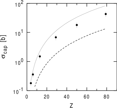
Figure 6: Pair production with capture for $Pb^{82+}$ (33 TeV) beams on several targets. The solid and dashed curves are theoretical calculations. See text for more details.

Replacing the Lorentz compressed electromagnetic fields by delta functions, and working with light cone variables, one has developed more elaborate calculations [82], recently. One still debates upon the proper treatment of Coulomb distortion of the lepton wavefunctions, and of production of n-pairs [82].

An important phenomenon occurs when the electron is captured in an atomic orbit of the projectile, or of the target. In a collider this leads to beam losses each time a charge modified nucleus passes by a magnet downstream [63]. A striking application of this process was the recent production of antihydrogen atoms using relativistic antiproton beams [83, 84]. Here the positron is produced and captured in an orbit of the antiproton. Early calculations for this process used perturbation theory [5, 58, 85, 86, 87, 88]. Some authors use non-perturbative approaches, e.g., coupled-channels calculations [76, 77, 78, 79, 80, 81]. Initially some discrepancy with perturbative calculations were found, but later it was shown that non-perturbative calculations agree with the perturbative ones at the 1% level (see, e.g., ref. [82, 89, 90, 91, 92, 68, 93]).

The expression

$$\sigma={3.3\pi Z^{8}\alpha^{6}r_{e}^{2}\over\exp\left(2\pi Z\alpha\right)-1}\left[\ln\left({0.681\gamma\over 2}\right)-{5\over 3}\right]$$ (27)

for pair production with electron capture in PHIC was obtained in ref. [5]. The term in the denominator is the main effect of the distortion of the positron wavefunction. It arises through the normalization of the continuum wavefunctions which accounts for the reduction of the magnitude of the positron wavefunction near the nucleus where the electron is localized (bound). Thus, the greater the $Z$, the less these wavefunctions overlap. Eq. 27 predicts a dependence of the cross section in the form $\sigma=A\ln\gamma+B$, where $A$ and $B$ are coefficients depending on the system. This dependence was used in the analysis of the experiment in ref. [57].

In recent calculations, attention was given to the correct treatment of the distortion effects in the positron wavefunction [95]. In figure 6 we show the recent experimental data of ref. [57] compared to eq. 27 and recent calculations [94, 95]. These calculations also predict a $\ln\gamma$ dependence but give larger cross sections than in ref. [5]. The comparison with the experimental data is not fair since atomic screening was not taken into account. When screening is present the cross sections will always be smaller up to a factor of 2 (see ref. [5]). The conclusion here is that pair production with electron capture is a process which is well treated in first order perturbation theory. However, eq. 27 is shown to be only a rough estimate of the cross section [94]. As with the production of free pairs, the main concern here is the correct treatment of distortion effects (multiphoton scattering) [94, 95].

The production of para-positronium in heavy ion colliders was calculated [66]. The cross section at RHIC is about 18 mb. This process is of interest due to the unusual large transparency of the parapositronium in thin metal layers.

The production of mesons in two- and three-photon collisions can be studied following the same formalism as used in QED for the production of positronium [96]. This is shown in the next section.

5 Photon-photon Fusion Mechanism

5.1 Meson Production

The production of heavy lepton pairs ($\mu^{+}\mu^{-}$, or $\tau^{+}\tau^{-}$), or of meson pairs (e.g., $\pi^{+}\pi^{-}$) can be calculated using the second of equation (1). One just needs the cross sections for $\gamma\gamma$ production of these pairs. Since they depend on the inverse of the square of the particle mass [63], the pair-production cross sections are much smaller in this case. The same applies to single meson production by $\gamma\gamma$ fusion. Low [97] showed that one can relate the particle production by two real photons (with energies $\omega_{1}$ and $\omega_{2}$, respectively) to the particle’s decay width, $\Gamma_{\gamma\gamma}$. Since both processes involve the same matrix elements, only the phase-space factors and polarization summations are distinct. Low’s formula is

$$\sigma(\omega_{1},\ \omega_{2})=8\pi^{2}(2J+1){\Gamma_{\gamma\gamma}\over M}\ \delta(4\omega_{1}\omega_{2}-M^{2})\ ,$$ (28)

where $J$, $M$, and $\Gamma_{M\rightarrow\gamma\gamma}$ are the spin, mass and two-photon decay width of the meson, $W$ is the c.m. energy of the colliding photons [63]. The delta-function accounts for energy conservation.

In ref. [5] the following equation was obtained for the production of mesons with mass $M$ in HI colliders:

$$\sigma={128\over 3}\ Z^{4}\alpha^{2}{\Gamma_{\gamma\gamma}\over M^{3}}\ \ln^{3}\left({2\gamma\delta\over MR}\right)\ ,$$ (29)

where $\delta=0.681...$ Later [99] it was shown that a more detailed account of the space geometry of the two-photon collision is necessary, specially for the heavier mesons. $R$ is a parameter which depends on the mass of the produced particle. If $M$ is much smaller than the inverse of a typical nuclear radius, then $R=1/M$, otherwise $R$ is the nuclear radius. These choices reflect the uncertainty relation in the direction transverse to the beam, as explained in ref. [5]. Since spin 1 particles cannot couple to two real photons [98], one expects that only spin 0 and spin 2 particles are produced.

In the next section we show how one can calculate meson production using the concepts of QED extended to include bound quark states [96].

Figure 7: Feynman graphs for two- and three-photon fusion in ultra-peripheral collisions of relativistic heavy ions.

5.2 Two-photon fusion in heavy ion colliders

In the laboratory frame the Fourier components of the classical electromagnetic field at a distance ${\bf b}/2$ of nucleus 1 with charge $Ze$ and velocity $\beta$, is given by (in our notation $q=(q_{0},{\bf q}_{t},q_{3})$, and $q_{3}\equiv q_{z}$)

$$A^{(1)}_{0}(q)=-8\pi^{2}Ze\ \delta(q_{0}-\beta q_{3}){e^{i{\bf q}_{t}.{\bf b}/2}\over{q^{2}_{t}+q_{3}^{2}/\gamma^{2}}}\ \ \ \ \ \ \ {\rm and}\ \ \ \ A^{(1)}_{3}=\beta A^{(1)}_{0}$$ (30)

For the field of nucleus 2, moving in the opposite direction, we replace $\beta$ by $-\beta$ and ${\bf b}$ by $-{\bf b}$ in the equations above. Although $\beta\simeq 1$ in relativistic colliders, it is important to keep them in the key places, as some of their combinations will lead to important $\gamma=(1-\beta^{2})^{-1/2}$ factors.

The matrix element for the production of positronium is directly obtained from the corresponding matrix element for the production of a free pair (see fig. 7(a)), with the requirement that $P_{+}=P_{-}=P/2$, where $P$ is the momentum of the final bound state. That is

$${\cal M} = {\cal M}_{1}+{\cal M}_{2}$$ (31)

$$= -ie^{2}\bar{u}({P\over 2})\left[\int{d^{4}q\over{(2\pi)^{4}}}\not\!\!A^{(1)}({P\over 2}-q){{\not\!q+M/2}\over{q^{2}-M^{2}/4}}\not\!\!A^{(2)}({P\over 2}+q)\right.$$

$$+ \left.\not\!\!A^{(1)}({P\over 2}+q){{\not\!q+M/2}\over{q^{2}-M^{2}/4}}\not\!\!A^{(2)}({P\over 2}-q)\right]v({P\over 2})\ ,$$

where $M$ is the positronium mass.

The treatment of bound states in quantum field theory is a very complex subject (for reviews, see [100, 101]). In our case, we want to use the matrix element for free-pair production and relate the results for the production of a bound-pair. A common trick used in this situation is to convolute the matrix element given above with the bound-state wave function. One can show (see, e.g., [102]) that this is equivalent to the use of projection operators of the form

$$\bar{u} \cdots v\longrightarrow\ {\Psi(0)\over 2\sqrt{M}}\ {\rm tr}\left[\cdots(\not\!\!P+M)i\gamma^{5}\right]\ ,\ \ {\rm and}$$

$$\bar{u} \cdots v\longrightarrow\ {\Psi(0)\over 2\sqrt{M}}\ {\rm tr}\left[\cdots(\not\!\!P+M)i\not\!\hat{e}^{*}\right]$$ (32)

where $\cdots$ is any matrix operator. The first equation applies to a spin 0 (parapositronium) and the second to spin 1 (orthopositronium) particles, respectively. In these equations $\Psi({\bf r})$ is the bound state wavefunction calculated at the origin, and $\hat{e}^{*}$ is the polarization vector, given by $\hat{e}^{*}_{\pm 1}=(0,1/\sqrt{2},\pm i/\sqrt{2},0)$ and $\hat{e}^{*}_{0}=(0,0,0,1)$.

Using eq. 32 in eq. 31, one gets for the parapositronium production

$${\cal M}=16i{\Psi(0)\over\sqrt{M}}\left(Z\alpha\right)^{2}\Big{|}{\bf P\times I}\Big{|}\ ,$$ (33)

where

$${\bf I}=\int{d^{2}q_{t}\ {\bf q}_{t}\over q_{t}^{2}+{\cal Q}^{2}}\ {1\over\left[\left({\bf P}_{t}/2+{\bf q}_{t}\right)^{2}+\omega_{1}^{2}/\gamma^{2}\right]}\ {1\over\left[\left({\bf P}_{t}/2-{\bf q}_{t}\right)^{2}+\omega_{2}^{2}/\gamma^{2}\right]}\ ,$$ (34)

with

$${\cal Q}^{2}={M^{2}\over 2}+{P_{t}^{2}\over 4}+{P_{z}^{2}\over 2\gamma^{2}}\simeq{M^{2}\over 2}+{P_{t}^{2}\over 4}$$ (35)

and

$$\omega_{1}={E/\beta-P_{z}\over 2}\ ,\ \ \ \omega_{2}={E/\beta+P_{z}\over 2}\ \ \ {\rm and}\ \ \ \ 4\omega_{1}\omega_{2}=M^{2}+P_{t}^{2}-P_{z}/\gamma^{2}\simeq M^{2}+P_{t}^{2}\ ,$$ (36)

where $E\equiv P_{0}$ is the total positronium energy.

We see that $\omega_{1}$ and $\omega_{2}$ play the role of the (real) photon energies. For real photons one expects $4\omega_{1}\omega_{2}=E^{2}$, as in eq. 28.

The two-photon fusion cross sections can be obtained by using

$$d\sigma=\sum_{\mu}\left[\int d^{2}b\ |{\cal M}(\mu)|^{2}\right]\ {d^{3}P\over(2\pi)^{3}\ 2E}$$ (37)

The positronium wavefunction at the origin is very well known. It is given by $\Big{|}\Psi(0)\Big{|}^{2}=M^{3}\alpha^{3}/64\pi$, where $M$ is the positronium mass.

Since the important impact parameters for the production of the positronium will be $b>1/m_{e}\gg R$, where $R$ is the nuclear radius, the integral over impact parameter can start from $b=0$. Thus, the integral over impact parameter in eq. 37 yields a delta function. Changing to the variables

$${\bf q}_{1t}={{\bf P}_{t}\over 2}-{\bf q}_{t}\ ,\ \ \ {\bf q}_{2t}={{\bf P}_{t}\over 2}+{\bf q}_{t}\ ,\ \ \ \ q_{1z}={P_{z}/2-q_{z}\over\gamma}\ ,\ \ \ \ q_{2z}={P_{z}/2+q_{z}\over\gamma}\ ,$$ (38)

eq. 37 becomes

$$E{d\sigma\over d^{3}P}={\zeta(3)\over\pi}\ {\sigma_{0}\over M^{2}}\ J_{B}\ ,$$ (39)

where

$$J_{B}={M^{2}\over\pi}\int{\bf A}^{2}\delta\left({\bf q}_{1t}+{\bf q}_{2t}-{\bf P}_{t}\right)d{\bf q}_{1t}d{\bf q}_{2t}\ ,$$ (40)

with

$${\bf A}={{\bf q}_{1t}\times{\bf q}_{2t}\over q_{1}^{2}q_{2}^{2}}\ {M^{2}\over M^{2}-q_{1}^{2}-q_{2}^{2}}\ ,\ \ \ \ \ \zeta(3)=1.202...\ ,\ \ \ \ {\rm and}\ \ \ \ \ \sigma_{0}={4Z^{4}\alpha^{7}\over M^{2}}\ .$$ (41)

We have included the zeta-function $\zeta(3)$ to take into account the production of the para-positronium in higher orbits, besides the production in the K-shell.

The equation 39 is equal to the equation obtained in ref. [66] for the production of the parapositronium, using an alternative method.

The integral in eq. 40 can be carried out analytically, reducing it to a 3-dimensional integral [96]. For RHIC, using $\gamma=108$ and $Au+Au$ collisions, one finds $\sigma=19.4$ mb. For the LHC , using $\gamma=3000$ and $Pb+Pb$ collisions, one finds $\sigma=116$ mb. These are in good agreement with the results (Born cross sections) of ref. [66]. Notice however, that Coulomb corrections are very important, due to the low mass of the electron and the positron [66]. When Coulomb corrections are included to the Born cross sections, the final values decrease by as much as 43% for RHIC and 27% for LHC. For meson production one expects that these corrections ere less relevant.

5.3 Production of $C=even$ Mesons

One can extend the calculation of the previous section to account for the production of mesons with spin $J=0$ and $J=2$ by the two-photon fusion mechanism. The following procedure is to be adopted:

1. Replace the electron-positron lines by quark-antiquarks in the diagram of figure 7(a).

2. $M$ in the following formulas will refer to the meson mass.

3. Replace $\alpha^{2}$ by $\alpha^{2}\ (2J+1)\ 3\sum_{i}Q_{i}^{4}$, where 3 accounts for the number of colors, and $Q_{i}$ is the fractional quark charge. These two last factors will cancel out when one expresses $\Big{|}\Psi(0)\Big{|}^{2}$ in terms of $\Gamma_{\gamma\gamma}$, the decay-width of the meson. To understand how this is done, lets discuss the basics of the annihilation process of a positronium (see also ref. [104]). With probability $\alpha^{2}$ the $e^{-}$ can fluctuate and emit a virtual photon with energy $~{}m_{e}$. The electron recoils and can travel up to a distance $\sim 1/m_{e}$ (or time $\sim m_{e}$) to meet the positron and annihilate. This occurs when $e^{-}$ and $e^{+}$ are both found close together in a volume of size $(1/m_{e})^{3}$, i.e., with a probability given by $|\Psi(0)|^{2}/m_{e}^{3}$. Thus, the annihilation probability per unit time (decay width) is $\Gamma\sim\alpha^{2}|\Psi(0)|^{2}/m_{e}^{2}$. Angular momentum conservation and CP invariance does not allow the ortho-positronium to decay into an even number of photons [98]. The description of the annihilation process given above is thus only appropriate for the para-positronium. A detailed QED calculation yields an extra $4\pi$ in the formula above. This yields $\Gamma_{\gamma\gamma}(^{1}S_{0})=8.03\times 10^{9}\ s^{-1}$, while the experimental value [107] is $7.99(11)\times 10^{9}\ s^{-1}$, in good agreement with the theory. For mesons, including the color and the charge factors, as described before, the relationship between $\Psi(0)$ and $\Gamma_{\gamma\gamma}$ arise due to the same reasons. One gets $\Gamma_{\gamma\gamma}=16\pi\alpha^{2}\Big{|}\Psi(0)\Big{|}^{2}/M^{2}\cdot 3\sum_{i}Q_{i}^{4}$.

   According to these arguments the connection between $\Gamma_{\gamma\gamma}$ and $\Big{|}\Psi(0)\Big{|}^{2}$, extended to meson decays, should be valid for large quark masses so that $1/m_{q}\ll\ \sqrt{<r^{2}>}$, where $\sqrt{<r^{2}>}$ is the mean size of the meson. Thus, it should work well for, e.g. charmonium states, $c\bar{c}$. In fact, Appelquist and Politzer [105] have generalized this derivation for the hadronic decay of heavy quark states, which besides other phase-space considerations amounts in changing $\alpha$ to $\alpha_{s}$, the strong coupling constant. This can be simply viewed as a way to get a constraint on the wavefunction $|\Psi(0)|^{2}$ (see, ref. [106]). One expects that these arguments are valid to zeroth order in quantum chromodynamics and in addition one should include relativistic corrections. But, as shown in [104], the inclusion of relativistic effects, summing diagrams to higher order in the perturbation series, is equivalent to solving the non-relativistic Schrödinger equation.

4. Change the integration variable to ${\bf q}_{1t}$ and ${\bf q}_{2t}$.

5. Introduce form factors $F(q_{1t})$ and $F(q_{2t})$ to account for the nuclear dimensions. This is a simple way to eliminate the integral over impact parameters and is justified ’a posteriori’, i.e., when one compares the results with those from other methods. These form factors will impose a cutoff in $q_{1t}$ and $q_{2t}$, so that

   $$q_{1t}\ ,\ \ q_{2t}\simeq{1\over R}\ll M\ ,$$ (42)

   where $R$ is a typical nuclear size. Taking $R=6.5$ fm, one gets $1/R\sim 30$ MeV. This is much smaller than the meson masses. As an outcome of this condition, one can replace ${\cal Q}^{2}\sim M^{2}/2$ in eq. 35.

According the procedures 1-5 one gets from eq. 39,

$${d\sigma\over dP_{z}} = {16(2J+1)\over\pi^{2}}{Z^{4}\alpha^{2}\over M^{3}}\ \Gamma_{\gamma\gamma}\ {1\over E}$$ (43)

$$\times \int d{\bf q}_{1t}d{\bf q}_{2t}\ ({\bf q}_{1t}\times{\bf q}_{2t})^{2}\ {\left[F_{1}(q_{1t}^{2})F_{2}(q_{2t}^{2})\right]^{2}\over\left(q_{1t}^{2}+\omega_{1}^{2}/\gamma^{2}\right)^{2}\left(q_{2t}^{2}+\omega_{2}^{2}/\gamma^{2}\right)^{2}}$$

Using eqs. 36 one has

$$E=\omega_{1}+\omega_{2}\ ,\ \ \ \ \omega_{1}-\omega_{2}=P_{z}\ ,\ \ \ \ \ {\rm and}\ \ \ \ \ \omega_{1}\omega_{2}=M^{2}/4$$

so that

$$dP_{z}=\left(1+{M^{2}\over 4\omega_{1}^{2}}\right)d\omega_{1}\ ,\ \ \ \ \ {\rm and}\ \ \ \ \ E={\omega_{1}^{2}+M^{2}/4\over\omega_{1}}\ .$$ (44)

Thus,

$${d\sigma\over d\omega_{1}}=\sigma^{(+)}\ {d{\cal N}_{2\gamma}(\omega_{1})\over d\omega_{1}}=\sigma^{(+)}\ {1\over\omega_{1}}\ n_{1}(\omega_{1})n_{2}(\omega_{2})\ ,$$ (45)

where

$$\sigma^{(+)}=8\pi^{2}(2J+1){\Gamma_{\gamma\gamma}\over M^{3}}\ \ \ \ {\rm and}\ \ \ \ \ n_{i}(\omega_{i})={2\over\pi}\ Z^{2}\alpha\ \int{dq\ q^{3}\ \left[F_{i}(q^{2})\right]^{2}\over\left(q^{2}+\omega_{i}^{2}/\gamma^{2}\right)^{2}}\ .$$ (46)

We notice that $n(\omega)$ is the frequently used form of the equivalent photon number which enters eq. 1. Thus, eqs. 45 and 46 are the result one expects by using the equivalent photon method, i.e., by using eqs. 28 and 1. This is an important result, since it shows that the projection method to calculate the two-photon production of mesons works even for light quark masses (i.e., for $\pi^{0}$). In this case there seems to be no justification for replacing the quark masses and momenta by half the meson masses and momenta, as we did for the derivation of eq. 43. This looks quite intriguing, but it is easy to see that the step 3 in our list of procedures adopted is solely dependent on the meson mass, not on the quark masses, i.e., if they are constituent, sea quarks, etc. Moreover, the projection method eliminates the reference to quark masses in the momentum integrals. The condition 42 finishes the job, by eliminating the photon virtualities and yielding the same result one would get with the equivalent photon approximation.

One can define a “two-photon equivalent number”, ${\cal N}_{2\gamma}(M^{2})$, so that $\sigma=\sigma^{(+)}{\cal N}_{2\gamma}(M^{2})$, where

$${\cal N}_{2\gamma}(M^{2})=\int d\omega{d{\cal N}_{2\gamma}\over d\omega}=\int{d\omega\over\omega}\ n_{1}(\omega)\ n_{2}\left({M^{2}\over 4\omega}\right)\ .$$ (47)

To calculate this integral one needs the equivalent photon numbers given by eq. 46. The simplest form factor one can use for this purpose is the ‘sharp-cutoff’ model, which assumes that

$$F(q^{2})=1\ \ {\rm for}\ \ q^{2}<1/R\ ,\ \ \ {\rm and}\ \ \ F(q^{2})=\ 0\ ,\ \ {\rm otherwise}\ .$$ (48)

In this case, one gets for the differential cross section

$${d\sigma\over d\omega} = \sigma^{(+)}\ {Z^{4}\alpha^{2}\over\pi^{2}\omega}\ \left[\ln\left(1+{\gamma^{2}\over\omega^{2}R^{2}}\right)-{1\over 1+\omega^{2}R^{2}/\gamma^{2}}\right]$$ (49)

$$\times \left[\ln\left(1+{16\gamma^{2}\omega^{2}\over M^{4}R^{2}}\right)-{1\over 1+M^{4}R^{2}/16\gamma^{2}\omega^{2}}\right]\ .$$

The spectrum possesses a characteristic $1/\omega$ dependence, except for $\omega\gg\gamma/R$, when it decreases as $1/\omega^{5}$.

When the condition $\gamma\gg MR$ is met, one can neglect the unity factors inside the logarithm in eq. 49, as well as the second term inside brackets. Then, doing the integration of 49 from $\omega=M^{2}R/4/\gamma$ to $\omega=\gamma/R$, we get eq. 29. But eq. 49 is an improvement over eq. 29. Eq. 29 is often used in the literature, but it is only valid for $\gamma\gg MR$. This relation does not apply to, e.g., the Higgs boson production ($M_{H^{0}}\sim 100$ GeV), as considered in ref. [103, 108, 109].

Figure 8: Two-photon luminosities (see definition in eq. 50) at RHIC and LHC. Dashed lines include a geometric correction.

For quantitative predictions one should use a more realistic form factor. The Woods-Saxon distribution, with central density $\rho_{0}$, size $R$, and diffuseness $a$ gives a good description of the densities of the nuclei involved in the calculation. For $Au$ we use $R=6.38$ fm, and $a=0.535$ fm, with $\rho_{0}$ normalized so that $\int d^{3}r\rho(r)=197$. For $Pb$ the appropriate numbers are 6.63 fm, 0.549 fm, and 208, respectively [110]. In table 2 we show the cross sections for the production of $C=even$ mesons at RHIC ($Au+Au$) and LHC ($Pb+Pb$) using the formalism described above.

Table 2: Cross sections for two-photon production of ($C=even$) mesons at RHIC ($Au+Au$) and at LHC ($Pb+Pb$).

meson	mass	$\Gamma_{\gamma\gamma}$	$\sigma^{(+)}$	${\cal N}_{2\gamma}^{RHIC}/10^{3}$	${\cal N}_{2\gamma}^{LHC}/10^{7}$	$\sigma^{RHIC}$	$\sigma^{LHC}$
	[MeV]	[keV]	[nb]			[$\mu$b]	[mb]
$\pi_{0}$	134	$7.8\times 10^{-3}$	99	49	2.8	4940	28
$\eta$	547	0.46	86	12	1.8	1000	16
$\eta^{\prime}$	958	4.2	147	5.1	1.4	746	21
$f_{2}(1270)$	1275	2.4	179	3.0	1.2	544	22
$a_{2}(1320)$	1318	1.0	67	2.9	1.1	195	8.2
$\eta_{c}$	2981	7.5	8.7	0.38	0.7	3.3	0.61
$\chi_{0c}$	3415	3.3	2.6	0.24	0.63	0.63	0.16
$\chi_{2c}$	3556	0.8	2.8	0.21	0.56	0.59	0.15

As pointed out in refs. [99, 111], one can improve the (classical) calculation of the two-photon luminosities by introducing a geometrical factor (the $\Theta$-function in ref. [99]), which affects the angular part of the integration over impact parameters. This factor takes care of the position where the meson is produced in the space surrounding the nuclei. In the approach described here the form factors also introduce a geometrical cutoff implying that the mesons cannot be produced inside the nuclei. However, it is not easy to compare both approaches directly, as one obtains a momentum representation of the amplitudes when one performs the integration over impact parameters to obtain eq. 43. But one can compare the effects of geometry in both cases by using equation 49. After performing the integral over $\omega$, one can rewrite it as

$$\sigma=\int ds{\cal L}(s)\sigma_{\gamma\gamma}(s)\ ,$$ (50)

where $s=4\omega_{1}\omega_{2}$ is the square of the center-of-mass energy of the two photons, $\sigma(s)$ is given by eq. 28, and ${\cal L}(s)$ is the “photon-photon luminosity”, given by

$${\cal L}(s) = {1\over s}\ {Z^{4}\alpha^{2}\over\pi^{2}}\int{d\omega\over\omega}\left[\ln\left(1+{\gamma^{2}\over\omega^{2}R^{2}}\right)-{1\over 1+\omega^{2}R^{2}/\gamma^{2}}\right]$$ (51)

$$\times \left[\ln\left(1+{16\gamma^{2}\omega^{2}\over s^{2}R^{2}}\right)-{1\over 1+s^{2}R^{2}/16\gamma^{2}\omega^{2}}\right]\ .$$

In figure 8 we compare the result obtained by eq. 51 and that of ref. [99]. The luminosities for RHIC ($Au+Au$) and for LHC ($Pb+Pb$) are presented. For RHIC the difference between the two results can reach 10% for very large meson masses (e.g. the Higgs), but one notices that for the LHC the two results are practically identical, the difference being of the order of 3%, or less, even for the Higgs production. Thus, the improved version of eq. 29, given by integrating eq. 49, is accurate enough to describe meson production by two-photon fusion. Other effects, like the interference between the electromagnetic and the strong interaction production mechanism in grazing collisions, must yield larger corrections to the (non-disruptive) meson production cross sections than a more elaborate description of geometrical effects.

One might think that the calculation above can be extended to the three-photon fusion by using the equivalent photon approximation that, as we have seen in this section, works so well for $C=even$ mesons. However, the introduction of a third photon leads to an additional integration, which implies that at least two of the exchanged photons cannot be treated as real ones. Nonetheless, the results of this section paves the way to the calculation of production of $C=odd$ mesons. Although the use of the projection technique to systems composed of light quarks is questionable, we have seen that it works, basically because of the relation 42, due to the inclusion of the nuclear form-factors.

5.4 Three-photon Mechanism: Vector mesons

Lets now consider the diagram of figure 7(b), appropriate for the fusion of three photons into a $C=odd$ particle. According to the Feynman rules, the matrix element for it is given by

$${\cal M}_{a} = e^{3}\bar{u}({P\over 2})\int{d^{4}q\over{(2\pi)^{4}}}\int{d^{4}k\over{(2\pi)^{4}}}\not\!\!A^{(1)}({P\over 2}-q){{\not\!q+M/2}\over{q^{2}-M^{2}/4}}$$ (52)

$$\times \not\!\!A^{(2)}(q-k){{\not\!k+M/2}\over{k^{2}-M^{2}/4}}\not\!\!A^{(2)}({P\over 2}+k)v({P\over 2})\ .$$

There will be 12 diagrams like this. But the upper photon leg in diagram of fig. 7(b) can be treated as a real photon, meaning that the equivalent photon approximation is valid for this piece of the diagram.

Figure 9: Feynman graphs for three-photon fusion in ultra-peripheral collisions of relativistic heavy ions.

A straightforward calculation yields

$${d\sigma\over dP_{z}} = 1024\pi\ \Big{|}\Psi(0)\Big{|}^{2}(Z\alpha)^{6}{1\over M^{3}E}\ \int{dq_{1t}\ q_{1t}^{3}\ \left[F(q_{1t}^{2})\right]^{2}\over\left(q_{1t}^{2}+\omega_{2}^{2}/\gamma^{2}\right)^{2}}$$ (53)

$$\times \int{dq_{2t}\ q_{2t}\ \left[F(q_{2t}^{2})\right]^{2}\over\left[q_{2t}^{2}+(2\omega_{1}-\omega_{2})^{2}/\gamma^{2}\right]^{2}}\left[\int{dk_{t}\ k_{t}\ F(k_{t}^{2})\over\left(k_{t}^{2}+(\omega_{1}-\omega_{2})^{2}/\gamma^{2}\right)}\right]^{2}$$

We now use the relationship between $E$ and $P_{z}$ to $\omega_{1}$ and $\omega_{2}$ and get rid of the meson wavefunction at the origin. The wavefunction $\Big{|}\Psi(0)\Big{|}^{2}$ cannot be related to the $\gamma\gamma$ decay widths. But, vector mesons can decay into $e^{+}e^{-}$ pairs. These decay widths are very well known experimentally. Following a similar derivation as for the $\gamma\gamma$-decay the $e^{+}e^{-}$ decay-width of the vector mesons can be shown [106] to be equal to $\Gamma_{e^{+}e^{-}}=16\pi\alpha^{2}\Big{|}\Psi(0)\Big{|}^{2}/3M^{2}\ (3\cdot\sum_{i}Q_{i}^{2})$. Inserting these results in the above equation, the factor $(3\cdot\sum_{i}Q_{i}^{2})$ will cancel out for the same reason as explained in section 3, and one gets

$${d\sigma\over d\omega}=\sigma^{(-)}\ \ {n(\omega)\over\omega}\ \ H(M,\omega)$$ (54)

where

$$\sigma^{(-)}=96\pi{\Gamma_{e^{+}e^{-}}\over M^{3}}\ ,$$ (55)

with $n(\omega)$ given by 46 and

$$H(M,\omega) = Z^{4}\alpha^{3}M^{2}\int{dq_{2t}\ q_{2t}\ \left[F(q_{2t}^{2})\right]^{2}\over\left[q_{2t}^{2}+(M^{2}/2\omega-\omega)^{2}/\gamma^{2}\right]^{2}}$$ (56)

$$\times \left[\int{dk_{t}\ k_{t}\ F(k_{t}^{2})\over\left(k_{t}^{2}+(M^{2}/4\omega-\omega)^{2}/\gamma^{2}\right)^{2}}\right]^{2}\ .$$

The above formulas should also be valid for the production of the ortho-positronium in ultra-peripheral collisions of relativistic heavy ions. For RHIC ($Au+Au$) one obtains $\sigma=11.2$ mb, while for the LHC ($Pb+Pb$) we get $\sigma=35$ mb. These numbers are also in good agreement with the results (in the Born approximation) given in ref. [66]. When one includes Coulomb corrections, as shown in ref. [66], the cross sections for orhto-positronium production is reduced by 40% for both RHIC and LHC. This is not considered in the present approach as we are mainly interested in vector meson production for which this effect should be smaller.

In table 3 we present the cross sections for the production of vector mesons by means of the three-photon fusion process are given.

Table 3: Cross sections for three-photon production of vector ($C=odd$) mesons at RHIC ($Au+Au$) and at LHC ($Pb+Pb$).

meson	mass [MeV]	$\Gamma_{e^{+}e^{-}}$ [keV]	$\sigma^{(-)}$ [nb]	$\sigma^{RHIC}$ [nb]	$\sigma^{LHC}$ [nb]
$\rho^{0}$	770	6.77	1740	137	1801
$\omega$	782	0.60	147	13	163
$J/\psi$	3097	5.26	21	31	423
$\Psi$’	3686	2.12	5	12	155

One sees that the cross sections for the production of vector mesons in ultra-peripheral collisions of relativistic heavy ions are small. They are not comparable to the production of vector mesons in central collisions. In principle, one would expect that the cross sections for three-photon production would scale as $(Z\alpha)^{3}$, which is an extra $Z\alpha$ factor compared to the two-photon fusion cross sections. However, the integral over the additional photon momentum decreases the cross section by several orders of magnitude.

In the next section we discuss the possibility to access information on the gluon distribution in nuclei using the abundant virtual photons in PHIC [112].

6 One-photon Production Mechanism

6.1 Vector Mesons and Gluon Distributions

One of main predictions of QCD is the transition from the confined/chirally broken phase to the deconfined/chirally symmetric state of quasi-free quarks and gluons, the so-called quark-gluon plasma (QGP). Recently the heavy ion collisions have provided strong evidence for the formation of a QGP [113], with the first results of RHIC marking the beginning of a collider era in the experiments with relativistic heavy ions, as well as the era of detailed studies of the characteristics of the QGP. Currently, distinct models associated to different assumptions describe reasonably the experimental data [114], with the main uncertainty present in these analysis directly connected with the poor knowledge of the initial conditions of the heavy ion collisions. Theoretically, the early evolution of these nuclear collisions is governed by the dominant role of gluons [115], due to their large interaction probability and the large gluonic component in the initial nuclear wave functions. This leads to a “hot gluon scenario”, in which the large number of initially produced energetic partons create a high temperature, high density plasma of predominantly hot gluons and a considerably number of quarks. Such extreme condition is expected to significantly influence QGP signals and should modify the hard probes produced at early times of the heavy ion collision. Consequently, a systematic measurement of the nuclear gluon distribution is of fundamental interest in understanding of the parton structure of nuclei and to determine the initial conditions of the QGP. Other important motivation for the determination of the nuclear gluon distributions is that the high density effects expected to occur in the high energy limit of QCD should be manifest in the modification of the gluon dynamics.

At small $x$ and/or large $A$ we expect the transition of the regime described by the linear dynamics (DGLAP, BFKL) (for a review, see e.g. ref. [116]), where only the parton emissions are considered, to a new regime where the physical process of recombination of partons becomes important in the parton cascade and the evolution is given by a nonlinear evolution equation. In this regime a Color Glass Condensate (CGC) is expected to be formed [117], being characterized by the limitation on the maximum phase-space parton density that can be reached in the hadron/nuclear wavefunction (parton saturation) and very high values of the QCD field strength $F_{\mu\nu}\approx 1/\sqrt{\alpha_{s}}$ [118]. In this case, the number of gluons per unit phase space volume practically saturates and at large densities grows only very slowly (logarithmically) as a function of the energy [119]. This implies a large modification of the gluon distribution if compared with the predictions of the linear dynamics, which is amplified in nuclear processes [120, 121, 122, 123].

Other medium effects are also expected to be present in the nuclear gluon distribution at large values of $x$: the antishadowing ($0.1<x<0.3$), the EMC effect ($0.3<x<0.7$) and the Fermi motion ($x>0.7$) [124, 125]. The presence of these effects is induced from the experimental data for the nuclear structure function which determines the behavior of the nuclear quark distributions and the use of the momentum sum rule as constraint. Experimentally, the behavior of the nuclear gluon distribution is indirectly determined in the lepton-nucleus processes in a small kinematic range of the fixed target experiments, with the behavior at small $x$ (high energy) completely undefined. This situation should be improved in the future with the electron-nucleus colliders at HERA and RHIC [126, 127], which probably could determine whether parton distributions saturate. However, until these colliders become reality we need to consider alternative searches in the current accelerators which allow us to constraint the nuclear gluon distribution. In this section we analyze the possibility of using peripheral heavy ion collisions as a photonuclear collider and therefore to determine the behavior of the gluon distribution.

A photon stemming from the electromagnetic field of one of the two colliding nuclei can penetrate into the other nucleus and interact with one or more of its hadrons, giving rise to photon-nucleus collisions to an energy region hitherto unexplored experimentally. For example, the interaction of quasireal photons with protons has been studied extensively at the electron-proton collider at HERA, with $\sqrt{s}=300$ GeV. The obtained $\gamma p$ center of mass energies extends up to $W_{\gamma p}\approx 200$ GeV, an order of magnitude larger than those reached by fixed target experiments. Due to the larger number of photons coming from one of the colliding nuclei in heavy ion collisions similar and more detailed studies will be possible in these collisions, with $W_{\gamma N}$ reaching 950 GeV for the Large Hadron Collider (LHC) operating in its heavy ion mode.

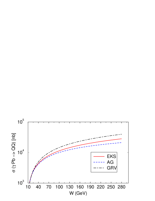
Figure 10: Energy dependence of the photoproduction of heavy quarks for distinct nuclear gluon distributions ($A=208$).

When a very hard photon from one equivalent swarm of photons penetrates the other nucleus it is able to resolve the partonic structure of the nucleus and to interact with the quarks and gluons. One of the basic process which can occur in the high energy limit is the photon-gluon fusion leading to the production of a quark pair. The main characteristic of this process is that the cross section is directly proportional to the nuclear gluon distribution. The analysis of this process in peripheral heavy ion collisions has been proposed many years ago [128] and improved in the Refs. [129, 130] (for a review, see ref. [131]). Here we reanalyze the charm photoproduction as a way to estimate the medium effects in $xG_{A}$ in the full kinematic region. We consider as input three distinct parameterizations of the nuclear gluon distribution. First, we consider the possibility that the nuclear gluon distribution is not modified by medium effects, i.e., $xG_{A}(x,Q^{2})=A\times xG_{N}(x,Q^{2})$, with the nucleon gluon distribution ($xG_{N}$) given by the GRV parameterization [132]. Moreover, we consider that $xG_{A}(x,Q^{2})=R_{G}\times xG_{N}(x,Q^{2})$, where $R_{G}$ parameterizes the medium effects as proposed by Eskola, Kolhinen and Salgado (EKS) [133]. The main shortcoming of these parameterizations is that these are based on the DGLAP evolution equations which are not valid in the small $x$ regime, where the parton saturation effects should be considered. In order to analyze the sensitivity of peripheral heavy ion collisions to these effects we consider as input the parameterization proposed by Ayala Filho and Gonçalves (AG) [134] which improves the EKS parameterization to include the high density effects.

One shortcoming of the analysis of photoproduction of heavy quarks in peripheral heavy ion collisions to constraint the nuclear gluon distribution is the linear dependence of the cross section with this distribution. This implies that only experimental data with a large statistics and small error will allow to discriminate the medium effects in the nuclear gluon distribution. Consequently, it is very important to analyze other possible processes which have a stronger dependence in $xG_{A}$. Here we propose the study of the elastic photoproduction of vector mesons in peripheral heavy ion collisions as a probe of the behavior of the nuclear gluon distribution. This process has been largely studied in $ep$ collisions at HERA, with the perturbative QCD predictions describing successfully the experimental data [116], considering a quadratic dependence of the cross section with the nucleon gluon distribution.

6.2 Photoproduction of Heavy Quarks

At high energies the dominant process occurring when the photon probes the structure of the nucleus is the photon-gluon fusion producing a quark pair. For heavy quarks the photoproduction can be described using perturbative QCD, with the cross section given in terms of the convolution between the elementary cross section for the sub-process $\gamma g\rightarrow Q\overline{Q}$ and the probability of finding a gluon inside the nucleus, i.e., the nuclear gluon distribution. Basically, the cross section for $c\overline{c}$ photoproduction is given by

$$\sigma_{\gamma g\rightarrow c\overline{c}}\,(s) = \int_{2m_{c}}^{\sqrt{s}}dM_{c\overline{c}}\frac{d\sigma_{c\overline{c}}}{dM_{c\overline{c}}}\,g_{A}(x,\mu)\,\,,$$ (57)

where $d\sigma_{c\overline{c}}/dM_{c\overline{c}}$ is calculable perturbatively, $M_{c\overline{c}}$ is the invariant mass of the $c\overline{c}$ pair with $M^{2}_{c\overline{c}}={\hat{s}}=xs$, $s$ is the squared CM energy of the $\gamma A$ system, $g_{A}(x,\mu)$ is the gluon density inside the nuclear medium, $\mu$ is the factorization scale ($\mu=\sqrt{M^{2}_{c\overline{c}}}$), and $m_{c}$ is the charm quark mass (we assume that $m_{c}=1.45$ GeV). Moreover, the differential cross section is [135]

$$\frac{d\sigma_{\gamma g\rightarrow c\overline{c}}}{dM_{c\overline{c}}}=\frac{4\pi\alpha\alpha_{s}e_{c}^{2}}{M^{2}_{c\overline{c}}}\Big{[}(1+\epsilon+\frac{1}{2}\epsilon^{2})\ln(\frac{1+\sqrt{1-\epsilon}}{1-\sqrt{1-\epsilon}})-(1+\epsilon)\sqrt{1-\epsilon}\Big{]}\,\,,$$ (58)

where $e_{c}$ is the charm charge and $\epsilon=4m_{c}^{2}/M_{c\overline{c}}^{2}$. From the above expression, we verify that the cross section is directly proportional to the nuclear gluon distribution, which implies the possibility to constraint its behavior from experimental results for photoproduction of heavy quarks.

Throughout this section we use the Born expression for the elementary photon-gluon cross section [eq. (58)]. QCD corrections to the Born cross section will not be considered here, although these corrections modify the normalization of the cross section by a factor of two. This is justified by the fact that we are interested in the relative difference between the predictions of the distinct nuclear gluon distributions, which should be not modified by the next-to-leading-order corrections.

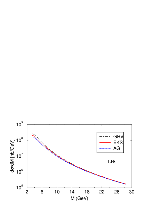
Figure 11: Differential cross section for $c\overline{c}$ production versus the invariant mass $M=M_{c\overline{c}}$. The photon-gluon fusion in the heavy-ion collision system ²⁰⁸Pb + ²⁰⁸Pb at LHC energy is considered.

In Fig. 10 we present the energy dependence of the photoproduction cross section. We focus our discussion on charm photoproduction instead of bottom photoproduction, since in this process smaller values of $x$ are probed. One verifies that different nuclear gluon distributions imply distinct behaviors for the cross section, with the difference between the predictions increasing with the energy. This is associated to the fact that at high energies we are probing the small $x$ behavior of $xG_{A}$, since $x\propto M_{c\overline{c}}/s$, where $M_{c\overline{c}}$ is the invariant mass of the photon-gluon system. Currently, only the region of small center of mass energy has been analyzed by the fixed target electron-nucleus experiments, not allowing a good constraint on medium effects present in the nuclear gluon distribution. Such situation should be improved in the future with electron-nucleus colliders at HERA and RHIC [124, 127].

Another possibility to study photoproduction of heavy quarks at large center of mass energies is to consider peripheral heavy ion collisions [128, 129, 130]. In this process the large number of photons coming from one of the colliding nuclei in heavy ion collisions will allow to study photoproduction, with $W_{\gamma N}$ reaching 950 GeV for the LHC. To determine the photoproduction of heavy quarks in peripheral heavy ion collisions the elementary photon-gluon cross section has to be convoluted with the photon energy distribution and the gluon distribution inside the nucleus:

$$\sigma(AA\rightarrow XXQ\overline{Q})=n(\omega)\otimes\sigma_{\gamma g\rightarrow Q\overline{Q}}\otimes xG_{A}(x,Q^{2})\,\,.$$ (59)

It is interesting to determine the values of $x$ which will be probe in peripheral heavy ion collisions. The Bjorken $x$ variable is given by $x=(M/2p)e^{-y}$, where $M$ is the invariant mass of the photon-gluon system and $y$ the center of momentum rapidity. For Pb + Pb collisions at LHC energies the nucleon momentum is equal to $p=3000$ GeV; hence $x=(M/6000\,{\rm GeV})e^{-y}$. Therefore, the region of small mass and large rapidities probes directly the small $x$ behavior of the nuclear gluon distribution. This demonstrates that peripheral heavy ion collisions at LHC represents a very good tool to determine the behavior of the gluon distribution in a nuclear medium, and in particular the low $x$ regime. Conversely, the region of large mass and small rapidities is directly associated to the region where the EMC and antishadowing effects are expected to be present. Similarly, for RHIC energies ($p=100$ GeV) the cross section will probe the region of medium and large values of $x$ ($x>10^{-2}$). For this kinematical region, the EKS and AG parameterizations are identical, which implies that the photoproduction of heavy quarks in peripheral heavy ion collisions at RHIC does not allows to constraint the high density effects. However, the study of this process at RHIC will be very interesting to determine the presence or not of the antishadowing and EMC effect in the nuclear gluon distribution.

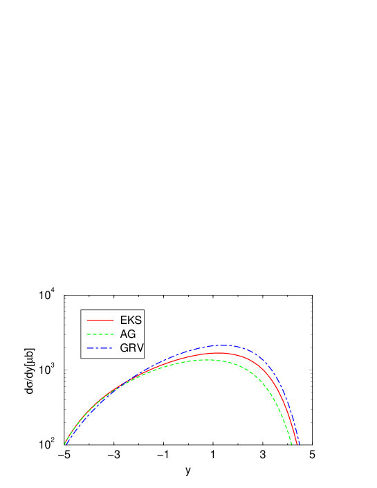
Figure 12: Rapidity distribution for the photoproduction of charm quarks in ²⁰⁸Pb + ²⁰⁸Pb collisions at LHC.

Fig. 11 shows the mass distribution in photoproduction of charm quarks in peripheral heavy ion collisions. We can see that the main difference between the predictions occur at small values of $M$, which is associated to the small $x$ region. Basically, we have that the predictions of the EKS parameterization are a factor 1.25 larger than the AG prediction in this region, while the prediction of Glück, Reya and Vogt (GRV) is a factor 2.4 larger. This result is consistent with the fact that the main differences between the parameterizations of the nuclear gluon distribution occur at small $x$ [134]. The difference between the predictions diminishes with the growth of the invariant mass, which implies that this distribution is not a good quantity to estimate the nuclear effects for medium and large $x$.

A better distribution to discriminate the behavior of the nuclear gluon distribution is the rapidity distribution, which is directly associated to the Bjorken $x$ variable, as discussed above. The rapidity distribution is calculated considering that $d\sigma/dy=\omega d\sigma/d\omega$. In Fig. 12 we show the rapidity distribution considering the three parameterizations of $xG_{A}$ as input. We have that the region of small rapidities probes the region of large $x$, while for large $y$ we directly discriminate the different predictions of $xG_{A}$ for small $x$. These results are coherent with this picture: as at large $x$ the EKS and AG predictions are identical, this region allows to estimate $R_{G}=xG_{A}/(AxG_{N})$ in the region of the antishadowing and EMC effects; at large $y$ the large difference between the parameterizations implies large modifications in the rapidity distribution, which should allow a clean experimental analysis.

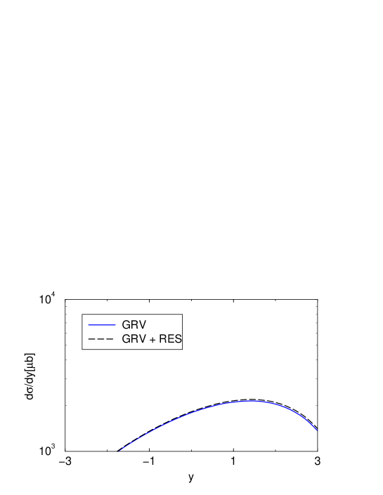
Figure 13: Rapidity distribution for the photoproduction of charm quarks in ²⁰⁸Pb + ²⁰⁸Pb collisions at LHC with (GRV+RES) and without (GRV) the inclusion of the resolved contribution.

A comment is in order here. In hard photon-hadron interactions the photon can behave as a pointlike particle in the so-called direct photon processes or it can act as a source of partons, which then scatter against partons in the hadron, in the resolved photon processes (for a recent review see ref. [136]). Resolved interactions stem from the photon fluctuation to a quark-antiquark state or a more complex partonic state, which are embedded in the definition of the photon structure functions. Recently, the process of jet production in photoproduction has been search of studies of the partonic structure of the photon (See e.g. [116]), and the contribution of the resolved photon for the photoproduction of charm has been estimated [137]. Basically, these studies shown that the partonic structure of the photon is particularly important in some kinematic regions (for example, the region of large transverse momentum of the charm pair [137]). Consequently, it is important to analyze if this contribution modifies, for instance, the results for the rapidity distribution, which is strongly dependent of nuclear gluon distribution. To leading order, beyond the process of photon-gluon fusion considered above, charm production can occur also in resolved photon interactions, mainly through the process $gg\rightarrow c\overline{c}$. Therefore, one needs to add in eq. (59) the resolved contribution given by

$$\sigma_{res}(AA\rightarrow XXQ\overline{Q})=n(\omega)\otimes x_{\gamma}G_{\gamma}(x_{\gamma},Q^{2})\otimes\sigma_{gg\rightarrow Q\overline{Q}}\otimes xG_{A}(x,Q^{2})\,\,,$$ (60)

where $x_{\gamma}$ denote the fraction of the photon momentum carried by its gluon component $x_{\gamma}G_{\gamma}$ and $\sigma_{gg\rightarrow Q\overline{Q}}$ the heavy quark production cross section first calculated in ref. [138]. Since the resolved contribution should be the same for the three nuclear parton distributions, Fig. 13 only shows the results obtained using the GRV parameterization for the nucleon. For the photon distribution we use the GRV photon parameterization [139], which predicts a strong growth of the photon gluon distribution at small $x_{\gamma}$. We can see that though this contribution is important in the photoproduction of heavy quarks, as shown in ref. [137], it is small in the rapidity distribution of charm quarks produced in peripheral heavy ion collisions. Therefore, the inclusion of the resolved component of the photon does not is not relevant for the use of this process as a probe of the nuclear gluon distribution.

It is important to salient that the potentiality of the photoproduction of quarks to probe the high density effects have been recently emphasized in ref. [140], where the color glass condensate formalism was used to estimate the cross section and transverse momentum spectrum. The authors have verified that the cross section is sensitive to the saturation scale which characterizes the colored glass. The results abovecorroborate the conclusion that this process is sensitive to the high density effects and the agreement between the predictions is expected in the kinematic region in which the transverse momentum of the pair $k_{t}$ is larger than the saturation scale $Q_{s}$. For $k_{t}<Q_{s}$ the collinear factorization to calculate the cross sections must be generalized, similarly to ref. [140].

6.3 Elastic Photoproduction of Vector Mesons

The production of vector mesons at HERA has become a rich field of experimental and theoretical research [for a recent review see, e.g. ref. [141]], mainly related with the question of whether perturbative QCD (pQCD) can provide an accurate description of the elastic photoproduction processes. At high energies the elastic photoproduction of vector mesons is a two-stage process: at first the photon fluctuates into the vector meson which then interacts with the target. For light vector mesons the latter process occurs similarly to the soft hadron-hadron interactions and can be interpreted within Regge phenomenology [142]. However, at large mass of the vector meson, for instance the mass of the $J/\Psi$ meson, the process is hard and pQCD can be applied [143]. In this case the lifetime of the quark-antiquark fluctuation is large compared with the typical interaction time scale and the formation of the vector meson only occur after the interaction with the target. In pQCD the interaction of the $q\overline{q}$ pair is described by the exchange of a color singlet system of gluons (two gluons to leading order) and, contrary to the Regge approach, a steep rise of the vector meson cross section is predicted, driven by the gluon distribution in the proton. Measurements of the elastic photoproduction of $J/\Psi$ mesons in $ep$ processes has been obtained by the H1 and ZEUS collaborations for values of center of mass energy below 300 GeV, demonstrating the steep rise of the cross section predicted by pQCD. This result motivates the extension of the pQCD approach used in electron-proton collisions to photonuclear processes.

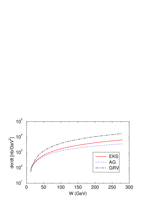
Figure 14: Energy dependence of the elastic photoproduction of $J/\Psi$ for distinct nuclear gluon distributions ($A=208$).

The procedure for calculating the forward differential cross section for photoproduction of a heavy vector meson in the color dipole approximation is straightforward. The calculation was performed some years ago to leading logarithmic approximation, assuming the produced vector-meson quarkonium system to be nonrelativistic [143] and improved in distinct aspects [144]. To lowest order the $\gamma A\rightarrow J/\Psi A$ amplitude can be factorized into the product of the $\gamma\rightarrow c\overline{c}$ transition, the scattering of the $c\overline{c}$ system on the nucleus via (colorless) two-gluon exchange, and finally the formation of the $J/\Psi$ from the outgoing $c\overline{c}$ pair. The heavy meson mass $M_{J/\Psi}$ ensures that pQCD can be applied to photoproduction. The contribution of pQCD to the imaginary part of the $t=0$ differential cross section of photoproduction of heavy vector mesons is given by [143]

$$\frac{d\sigma(\gamma A\rightarrow J/\Psi A)}{dt}|_{t=0}=\frac{\pi^{3}\Gamma_{ee}M_{J/\Psi}^{3}}{48\alpha}\frac{\alpha_{s}^{2}(\overline{Q}^{2})}{\overline{Q}^{8}}\times[xG_{A}(x,\overline{Q}^{2})]^{2}\,\,,$$ (61)

where $xG_{A}$ is the nuclear gluon distribution, $x=4\overline{Q}^{2}/W^{2}$ with $W$ the center of mass energy and $\overline{Q}^{2}=M_{J/\Psi}^{2}/4$. Moreover, $\Gamma_{ee}$ is the leptonic decay width of the vector meson. The total cross section is obtained by integrating over the momentum transfer $t$,

$$\sigma(\gamma A\rightarrow J/\Psi A)=\frac{d\sigma(\gamma A\rightarrow J/\Psi A)}{dt}|_{t=0}\,\int_{t_{min}}^{\infty}dt\,|F(t)|^{2}\,\,\,,$$ (62)

where $t_{min}=(M_{J/\Psi}^{2}/2\omega)^{2}$ and $F(t)=\int d^{3}r\ \rho(r)\ \exp(i{\bf q}\cdot{\bf r})$ is the nuclear form factor for the matter distribution.

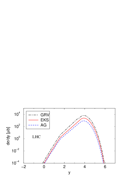
Figure 15: The rapidity distribution for elastic photoproduction of $J/\Psi$ at LHC considering distinct nuclear gluon distributions ($A=208$).

A comment is in order here. Although some improvements of the expression (61) have been proposed in the literature [144], these modifications do not change the quadratic dependence on $xG_{A}$.

The main characteristic of the elastic photoproduction of vector mesons is the quadratic dependence on the gluon distribution, which makes it an excellent probe of the behavior of this distribution. In Fig. 14 we show the energy dependence of the differential cross section [eq. (61)], considering the three distinct nuclear gluon distributions discussed above. One obtains larger differences between the predictions than obtained in photoproduction of heavy quarks, mainly at large values of energy. This result motivates experimental analysis of elastic $J/\Psi$ photoproduction in photonuclear processes at high energies. Although the future electron ion colliders (HERA-A and eRHIC) should probe this kinematic region, here we show that this can also be done with peripheral heavy ion collisions.

Following similar steps used in photoproduction of heavy quarks, photons coming from one of the colliding nuclei may interact with the other. For elastic photoproduction of $J/\Psi$ one can consider that this photon decays into a $c\overline{c}$ pair which interacts with the nuclei by the two gluon exchange. After the interaction, this pair becomes the heavy quarkonium state. Consequently, the total cross section for $J/\Psi$ production in peripheral heavy ion collisions is obtained by integrating the photonuclear cross section [eq. (62)] over the photon spectrum, resulting

$$\sigma(AA\rightarrow AAJ/\Psi)=\int\frac{d\omega}{\omega}\ n(\omega)\frac{d\sigma(\gamma A\rightarrow J/\Psi A)}{dt}|_{t=0}\,\int_{t_{min}}^{\infty}dt\,|F(t)|^{2}\,\,.$$ (63)

Table 4: The total cross section $\sigma(AA\rightarrow AAJ/\Psi)$ for different nuclear gluon distributions. Results for LHC.

Gluon Distribution	LHC
GRV	$6.584$ mb
EKS	2.452 mb
AG	0.893 mb

Table 4 presents the total cross section considering as input the distinct nuclear gluon distributions and LHC energies. Although these numbers will be modified by the inclusion of higher order corrections for the cross section [144], the difference between the predictions should not be altered. One verifies that due to the large number of equivalent photons and the large center of mass energies of the photon-nucleus system, the cross section for this process is large, which allows an experimental verification of these predictions. Also, in peripheral heavy ion collisions the multiplicity is small what might simplify the experimental analysis. Moreover, the difference between the predictions is significant. For RHIC energies, the cross section for this process is small and probably an experimental determination will be very hard.

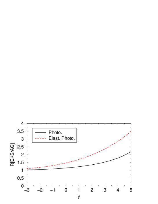
Figure 16: Rapidity behavior of the ratio between the EKS and AG predictions for photoproduction of charm quarks and elastic photoproduction of $J/\Psi$.

In fig. 15 the rapidity distribution for $J/\Psi$ production at LHC energies is shown. In this case, the final state rapidity is determined by

$$y=\frac{1}{2}\ln\frac{\omega}{\sqrt{|t_{min}|}}=\ln\frac{2\omega}{M_{J/\Psi}}\,\,.$$ (64)

Similarly to the heavy quark photoproduction, the large $y$ region probes the behavior of $xG_{A}$ at small $x$, while the region of small $y$ probes medium values of $x$. One concludes that the rapidity distribution for elastic production of $J/\Psi$ at RHIC allows to discriminate between the GRV and EKS prediction, with the AG prediction being almost identical to the latter. For LHC one finds a large difference between the distributions, mainly in magnitude, which will allow to estimate the magnitude of the EMC, antishadowing and high density effects.

Finally, fig. 16 compares the photoproduction of heavy quarks and the elastic photoproduction of $J/\Psi$ in peripheral heavy ion collisions as a possible process to constraint the behavior of the nuclear gluon distribution. The rapidity distribution of the ratio

$$R[EKS/AG]\equiv\frac{d\sigma}{dy}[EKS]/\frac{d\sigma}{dy}[AG]\,\,,$$ (65)

is shown where we consider the EKS and AG parameterizations as inputs of the rapidity distributions. One confirms that the analysis of the elastic photoproduction of $J/\Psi$ at medium and large rapidities is a potential process to determinate the presence and estimate the magnitude of the high density effects.

7 Final Remarks

The possibility to produce a Higgs boson via $\gamma\gamma$ fusion was suggested in ref. [103, 108]. The cross sections for LHC are of order of 1 nanobarn, about the same as for gluon-gluon fusion. But, the two-photon processes can also produce $b\bar{b}$ pairs which create a large background for detecting the Higgs boson. A good review of these topics was presented in ref. [145].

The excitation of a hadron in the field of a nucleus is another useful tool to study the properties of hadrons. It has been used for example to obtain the lifetime of the $\Sigma_{0}$ particle by measuring the (M1) excitation cross section for the process $\gamma+\Lambda\rightarrow\Sigma_{0}$ [146]. The vertex $\gamma\rightarrow 3\pi$ has been investigated [147] in the reaction of pion pair production by pions in the nuclear Coulomb field: $\pi^{-}+Z\rightarrow\pi^{-}+\pi^{0}+Z$. Also, the $\pi^{-}$ polarizability has been studied in the reaction $\pi^{-}+Z\rightarrow\pi^{-}+\gamma+Z$ [148]. Other unexplored possibilities includes the excitation of a nucleon to a $\Delta$-particle in the field of a heavy nucleus in order to disentangle the $M1$ and $E2$ parts of the excitation.

As for meson-production in PHIC there are several planned experiments at RHIC, as well as for the future LHC [149]. These machines were designed to study hadronic processes. But, as have shown in this brief review, they can also be used for studying very interesting phenomena induced in peripheral collisions.

References

- [1] C.A. Bertulani and G. Baur, Physics Today, March 1994, p. 22.
- [2] E. Fermi, Z. Physik 29, 315 (1924).
- [3] K. F. Weizsacker, Z. Physik , 612 (1934); E. J. Williams, Phys. Rev. 45, 729 (1934).
- [4] C.A.Bertulani and G. Baur, Nucl. Phys. A442 (1985) 73.
- [5] C.A. Bertulani and G. Baur, Physics Reports 163 (1988) 299.
- [6] G. Baur, K. Hencken, D. Trautmann, S. Sadovsky, Y. Kharlov, Phys. Rep. 364, 359 (2002).
- [7] C.A. Bertulani, L.F. Canto and M.S. Hussein, Phys. Rep. 226, 282 (1993).
- [8] T. Glasmacher, Ann. Rev. Nucl. Part. Sci. 48 (1998) 1.
- [9] T. Aumann, P.F. Bortignon, H. Emling, Ann. Rev. Nucl. Part. Sci. 48, 282 (1998).
- [10] C.A. Bertulani and V.Yu. Ponomarev, Phys. Reports 321, 139 (1999).
- [11] S.A. Austin and G.F. Bertsch, Scientific American, 272, 62 (1995) 62
- [12] P. G. Hansen, A. S. Jensen, and B. Jonson, Ann. Rev. Nucl. Part. Sci. 45, 591 (1995).
- [13] G. Baur, C.A. Bertulani and D.M. Kalassa, Nucl. Phys. A550, 527 (1992).
- [14] K. Ieki, et al., Phys. Rev. Lett. 70 (1993) 730.
- [15] G.F. Bertsch and C.A. Bertulani, Nucl. Phys. A556, 136 (1993); Phys. Rev. C49, 2834 (1994).
- [16] M.S.Hussein, R.A.Rego and C.A. Bertulani, Phys. Reports 201, 279 (1991).
- [17] H. Esbensen, G.F. Bertsch and C.A. Bertulani, Nucl. Phys. A581, 107 (1995).
- [18] T. Kido, K. Yabana and Y. Suzuki, Phys.Rev. C53, 2296 (1996).
- [19] D.D. Clayton, Principles of Stellar Evolution and Nucleosynthesis, McGraw-Hill, New York, 1968.
- [20] C. Rolfs and W.S. Rodney, Cauldrons in the Cosmos, Chicago Press, Chicago, 1988.
- [21] G.Baur, C.A.Bertulani and H.Rebel, Nucl. Phys. A458, 188 (1986).
- [22] C.A.Bertulani and L.F.Canto, Nucl. Phys. A539, 163 (1992).
- [23] C.A. Bertulani, Z. Phys. A356, 293 (1996).
- [24] F.M. Nunes and I.J. Thompson, Phys. Rev. C59, 2652 (1999).
- [25] V. S. Melezhik and D. Baye, Phys. Rev. C59, 3232 (1999).
- [26] H. Utsunomia, Y. Tokimoto, T. Yamagata, M. Ohta, Y. Aoki, K. Hirota, K. Ieki, Y. Iwata, K. Katori, S. Hamada, Y.-W. Lui, R. P. Schmitt, S. Typel and G. Baur, Nucl. Phys. A654, 928 (1999).
- [27] S. Typel, H. H. Wolter, Z. Naturforsch. 54 a, 63 (1999).
- [28] N. Iwasa, et al., Phys. Rev. Lett. 83 (1999) 2910
- [29] P. Descouvemont and D. Baye, Nucl. Phys. A567, 341 (1994).
- [30] B. Davids, D. W. Anthony, T. Aumann, Sam M. Austin, T. Baumann, D. Bazin, R. R. C. Clement, C. N. Davids, H. Esbensen, P. A. Lofy, T. Nakamura, B. M. Sherrill, J. Yurkon, Phys.Rev.Lett. 86, 2750 (2001).
- [31] B. Davids, D.W. Anthony, Sam M. Austin, D. Bazin, B. Blank, J.A. Caggiano, M. Chartier, H. Esbensen, P. Hui, C.F. Powell, H. Scheit, B.M. Sherrill, M. Steiner, P. Thirolf, Phys. Rev. Lett. 81, 2209 (1998).
- [32] B. Davids, Sam M. Austin, D. Bazin, H. Esbensen, B. M. Sherrill, I. J. Thompson, and J. A. Tostevin, Phys. Rev. C63, 065806 (2001).
- [33] H. Esbensen and G. Bertsch, Nucl. Phys. A600, 37 (1996).
- [34] G. Baur and H. Rebel, Annu. Rev. Nucl. Part. Sc. 46, 321 (1996).
- [35] J. Kiener, A. Lefebre, P. Aguer, C.O. Bacri, R. Bimbot, G. Bogaert, B. Borderie, F. Claper, A. Coc, D. Disdier, S. Fortier, C. Grunberg, L. Klaus, I. Linck, G. Pasquier, M.F. Rivet, F. StLaurent, C. Stephan, L. Tassangot and J.P. Thibaud, Nucl. Phys. A552, 66 (1993).
- [36] J. Kiener, H. J. Gils, H. Rebel, S. Zagromski, G. Gsottschneider, N. Heide, H. Jelitto, J. Wentz and G. Baur, Phys. Rev. C44, 2195 (1991).
- [37] T. Motobayashi et al., Phys. Lett B264, 259 (1991).
- [38] A. Lefebre et al., Nucl. Phys. A595, 69 (1995).
- [39] V. Tatischeff, J. Kiener, P. Aguer, and A. Lefebvre Phys. Rev. C51, 2793 (1995).
- [40] G. Baur and C.A. Bertulani, Phys. Lett. B 174 (1986) 23; Nucl. Phys. A 482 (1988) 313; Phys. Rev. C 34 (1986) 1654; Proc. Int. School of Heavy Ion Physics, Erice, Italy, October 1986, Plenum Press, ed. by R.A. Broglia and G.F. Bertsch, p. 331.
- [41] W. Llope and P. Braun-Munzinger, Phys. Rev. C 45 (1992) 799; W. Llope, Ph. D. dissertation, SUNY at Stony Brook, 1992, and private communication.
- [42] J. Ritman, F. D. Berg, W. K hn, V. Metag, R. Novotny, M. Notheisen, P. Paul, M. Pfeiffer, and O. Schwalb, H. L hner and L. Venema, A. Gobbi, N. Herrmann, K. D. Hildenbrand, J. M sner, R. S. Simon, K. Teh, J. P. Wessels, and T. Wienold, Phys. Rev. Lett. 70, 533 (1993).
- [43] R. Schmidt, Th. Blaich, Th. W. Elze, H. Emling, H. Freiesleben, K. Grimm, W. Henning, R. Holzmann, J. G. Keller, H. Klingler, R. Kulessa, J. V. Kratz, D. Lambrecht, J. S. Lange, Y. Leifels, E. Lubkiewicz, E. F. Moore, E. Wajda, W. Prokopowicz, Ch. Sch tter, H. Spies, K. Stelzer, J. Stroth, W. Walus, H. J. Wollersheim, M. Zinser, E. Zude, Phys. Rev. Lett. 70, 1767 (1993).
- [44] T. Aumann, J. V. Kratz, and E. Stiel, K. S mmerer, W. Br chle, M. Sch del, and G. Wirth, M. Fauerbach and J. Hill, Phys. Rev. C47, 1728 (1993).
- [45] K. Boretzky, J. Stroth, E. Wajda, T. Aumann, Th. Blaich, J. Cub, Th. W. Elze, H. Emling, W. Henning, R. Holzmann, H. Klingler, R. Kulessa, J. V. Kratz, D. Lambrecht, Y. Leifels, E. Lubkiewicz, K. Stelzer, W. Walus, M. Zinser, E. Zude, Phys. Lett. B384, 30 (1996 ).
- [46] A. Gr nschloss, K. Boretzky, T. Aumann , C. A. Bertulani, J. Cub, W. Dostal, B. Eberlein, Th. W. Elze, H. Emling, J. Holeczek, R. Holzmann, M. Kaspar, J. V. Kratz, R. Kulessa, Y. Leifels, A. Leistenschneider, E. Lubkiewicz, S. Mordechai, I. Peter, P. Reiter, M. Rejmund, H. Simon, K. Stelzer, A. Surowiec, K. S mmerer, J. Stroth, E. Wajda, W. Walus, S. Wan, H. J. Wollersheim, Phys. Rev. C60, 051601 (1999).
- [47] K. Boretzky, T. Aumann, J. Cub, Th. W. Elze , H. Emling, A. Gr nschloss, R. Holzmann, S. Ilievski, R. Kulessa, J. V. Kratz, Y. Leifels, A. Leistenschneider, E. Lubkiewicz, J. Stroth, E. Wajda, W. Walus, Nucl. Phys. A649, 235c (1999).
- [48] S. Ilievski, T. Aumann, K. Boretzky, J. Cub, W. Dostal, B. Eberlein, Th. W. Elze, H. Emling, A. Gr nschloss, J. Holeczek, R. Holzmann, C. Kozhuharov, J. V. Kratz, R. Kulessa, Y. Leifels, A. Leistenschneider, E. Lubkiewicz, T. Ohtsuki, P. Reiter, H. Simon, K. Stelzer, J. Stroth, A. Surowiec, E. Wajda, W. Walus , Nucl. Phys. A687 , 178c (2001).
- [49] C. A. Bertulani, L. F. Canto, M. S. Hussein, and A. F. R. de Toledo Piza, Phys. Rev. C53, 334 (1996).
- [50] M. S. Hussein, A. F. R. de Toledo Piza, and O. K. Vorov Phys. Rev. C59, R1242 (1999).
- [51] A. F. R. de Toledo Piza, M. S. Hussein, B. V. Carlson, C. A. Bertulani, L. F. Canto, and S. Cruz-Barrios Phys. Rev. C59, 3093 (1999); B. V. Carlson, L. F. Canto, S. Cruz-Barrios, M. S. Hussein, and A. F. R. de Toledo Piza Phys. Rev. C59, 2689 (1999); B. V. Carlson and M. S. Hussein Phys. Rev. C59, R2343 (1999); B. V. Carlson, M. S. Hussein, A. F. R. de Toledo Piza, and L. F. Canto Phys. Rev. C60, 014604 (1999).
- [52] D. T. de Paula, T. Aumann, L. F. Canto, B. V. Carlson, H. Emling, and M. S. Hussein, Phys. Rev. C64, 064605 (2001).
- [53] I.A. Pshenichnov, J.P. Bondorf, I.N. Mishustin, A. Ventura and S. Masetti, Phys.Rev. C64, 024903 (2001).
- [54] A.J. Baltz, M.J. Rhoades-Brown, and J. Weneser, Phys. Rev E54, 4233 (1996); A.J. Baltz, C. Chasman and S.N. White, Nucl. Instrum. Meth, A417, 1 (1998); S.N. White, Nucl. Instrum. Meth. A409, 618 (1998).
- [55] M. Chiu, A. Denisov, E. Garcia, J. Katzy, A. Makeev, M. Murray, and S. White, Phys. Rev. Lett. 89, 012302 (2002).
- [56] A.J. Baltz, physics/0102045; see also, A.B. Voitkov, C. Müller, and N. Grün, Phys. Rev. A62, 062701 (2000).
- [57] H.F. Krause et al., Phys. Rev. Lett. 80 (1998) 1190.
- [58] R. Anholt and U. Becker, Phys. Rev. A36 (1987) 4628.
- [59] J. Eichler and W. Meyerhof, Relativistic Atomic Collisions (Academic Press, San Diego, 1995).
- [60] R. Anholt and H. Gould, in AAdvances in Atomic and Molecular Physics (Academic Press, San Diego, 1986), p. 315.
- [61] U. Becker, N. Grün and W. Scheid, J. Phys. B16 (1983) 1967; U. Becker, PhD. Thesis, Giessen (1986).
- [62] C. Bottcher and M.R. Strayer, Phys. Rev. Lett. 54 (1985) 669.
- [63] G. Baur and C.A. Bertulani, Z. Phys. A330 (1988) 77; C.A. Bertulani and G. Baur, Nucl. Phys. A505 (1989) 835.
- [64] I.F. Ginzburg, G.L. Kotkin, S.I. Polityko and V.G. Serbo, Phys. Rev. Lett. 68 (1992) 788; Phys. Lett. B286 (1992) 392; Z. Phys. C60 (1993) 737.
- [65] V. Serbo, private communication.
- [66] G.L. Kotkin, E.A. Kuraev, A. Schiller and V.G. Serbo, Phys. Rev. C59 (1999) 2734
- [67] U. Eichmann, J. Reinhardt, and W. Greiner, Phys. Rev. A 61, 062710 (2000).
- [68] A. Baltz, F. Gelis, L. McLerran and A. Peshier, Nucl. Phys. A695, 395 (2001).
- [69] A.J. Baltz, M.J. Rhoades-Brown, and J. Weneser, Phys. Rev. A 44, 5569 (1991); Phys. Rev. A 48, 2002 (1993); Phys. Rev. A 47, 3444 (1993); Phys. Rev. A 50, 4842 (1994); A.J. Baltz, Phys. Rev. A 52, 4970 (1995).
- [70] C.A. Bertulani, Phys. Rev. A63, 062706 (2001).
- [71] A.B. Voitkiv, C. Müller, and N. Grün, Phys. Rev. A62, 062701 (2000).
- [72] W.H. Furry and J.F. Carlson, Phys. Rev. 44, 238 (1933).
- [73] L.D. Landau and E.M. Lifshitz, Phys. Zs. Sowjet. 6, 244 (1934).
- [74] H.J. Bhabha, Proc. R. Soc. London Ser. A152, 559 (1935).
- [75] Y. Nishina, S. Tomonaga and M. Kobayashi , Sci. Pap. Phys. Chem. Res. 27, 137 (1935).
- [76] C. Bottcher and M.R. Strayer, Phys. Rev. D39, 1330 (1989); J. Phys. G16, 975 (1990); Phys. Lett. B237 (1990) 175.
- [77] G. Baur, Phys. Rev. D41, 3535 (1990); Phys. Rev. A42, 5736 (1990).
- [78] M.J. Rhoades-Brown and J. Weneser, Phys. Rev. A4, 33 (1991).
- [79] C. Best, W. Greiner and G. Soff, Phys. Rev. A46 (1992) 261.
- [80] M. Vidović, M. Greiner, C. Best and G. Soff, Phys. Rev. C47, 2308 (1993).
- [81] K. Hencken, D. Trautmann and G. Baur, Phys. Rev. A51 (1995) 998; A51, 1874 (1995).
- [82] A.J. Baltz, Phys. Rev. Lett. 78 (1997) 1231.
- [83] G. Baur et al., Phys. Lett. B368, 351 (1996).
- [84] G. Blanford et al., Phys. Rev. Lett. 80, 3037 (1998).
- [85] U. Becker, J. Phys. B20, 6563 (1987).
- [86] K. Momberger, N. Grün and W. Scheid, Z. Phys. D18, 133 (1991).
- [87] K. Rumrich, G. Soff and W. Greiner, Phys. Rev. A47 , 215 (1993).
- [88] K. Momberger, A. Belkacem and A.H. Sorensen, Europhys. Lett. 32, 401 (1995).
- [89] A.J. Baltz and L. McLerran, Phys. Rev. C58, 1679 (1998).
- [90] B. Segev and J.C. Wells, Phys. Rev. A57, 1849 (1998).
- [91] D.Yu. Ivanov, A. Schiller, V.G. Serbo, Phys. Lett. B454, 155 (1999).
- [92] U. Eichmann, J. Reinhardt, S. Schramm and W. Greiner, Phys. Rev. A59, 1223 (1999).
- [93] R.N. Lee and A.J. Milstein, hep-ph/0103212.
- [94] C. A. Bertulani and D. Dolci, Nucl. Phys. A683, 635 (2001).
- [95] H. Meier, Z. Halabuka, K. Hencken, D. Trautmann and G. Baur, e-print nucl-th/0008020.
- [96] C.A. Bertulani and F. Navarra, Nucl. Phys. A703, 861 (2002).
- [97] F.E. Low, Phys. Rev. 120, 582 (1960).
- [98] C.N. Yang, Phys. Rev. 77, 242 (1950); L. Wolfenstein and D.G. Ravenhall, Phys. Rev. 88, 279 (1952).
- [99] G. Baur and L.G. Ferreira Filho, Nucl. Phys. A518, 786 (1990).
- [100] G.T. Bodwin, D.R. Yennie and M.A. Gregorio, Rev. Mod. Phys. 57, 723 (1985).
- [101] “Theory of hydrogenic bound states”, J. Sapirstein and D.R. Yennie, in “Quantum electrodynamics”, edited by T. Kinoshita, World Scientific, Singapore (1990).
- [102] V.A. Novikov et al., Phys. Rep. 41C, 1 (1978).
- [103] E. Papageorgiu, Phys. Rev. D40, 92 (1989).
- [104] V. B. Berestetskii, E.M. Lifshitz and L.P. Pitaevskii, Quantum Electrodynamics, 2nd edition, Pergamon, Oxford, 1982.
- [105] T. Appelquist and H.D. Politzer, Phys. Rev. Lett. 34, 43 (1975).
- [106] R.P. Royen and V.F. Weisskopf, Nuovo Cim. A50, 617 (1967).
- [107] E.D. Theriot, Jr., R. H. Beers, V. W. Hughes, and K. O. H. Ziock, Phys. Rev. A2, 707 (1970).
- [108] M. Grabiak, B. Müller, W. Greiner and P. Koch, J. Phys. G15, L25 (1989).
- [109] C.G. Roldão and A.A. Natale, Phys. Rev. C61, 064907 (2000).
- [110] C.W. de Jager, H. de Vries and C. de Vries, Atomic Data and Nuclear Data Tables 14, 479 (1974).
- [111] R.N. Cahn and J.D. Jackson, Phys. Rev. D42, 3690 (1990).
- [112] V.P. Gonçalves and C.A. Bertulani, Phys. Rev. C65, 054905 (2002).
- [113] See, e.g., U. Heinz, Nuc. Phys. A 685, 414 (2000).
- [114] K. J. Eskola, Proceedings ”Quark Matter 2001”, Nuc. Phys. A (in press), hep-ph/0104058.
- [115] See, e.g., K. Geiger., Phys. Rep. 258, 237 (1995); X.-N Wang., Phys. Rep. 280, 287 (1997).
- [116] H. Abramowicz and A. C. Caldwell, Rev. Mod. Phys. 71, 1275 (1999).
- [117] E. Iancu, A. Leonidov and L. McLerran, Nuc. Phys. A692, 583 (2001).
- [118] A. H. Mueller, Nucl. Phys. B558, 285 (1999).
- [119] M. B. Gay Ducati and V. P. Gonçalves, Phys. Lett. B502, 92 (2001).
- [120] A. L. Ayala, M. B. Gay Ducati and E. M. Levin. Nucl. Phys. B493, 305 (1997).
- [121] E. Gotsman, E. Levin, U. Maor, L. McLerran and K. Tuchin, Nuc. Phys. A683, 383 (2000).
- [122] M. B. Gay Ducati and V. P. Gonçalves, Phys. Lett. B466, 375 (1999).
- [123] V. P. Gonçalves, Phys. Lett. B495, 303 (2000).
- [124] M. Arneodo, Phys. Rep. 240, 301 (1994).
- [125] G. Piller and W. Weise, Phys. Rep. 330, 1 (2000).
- [126] M. Arneodo et al., Future Physics at HERA. Proceedings of the Workshop 1995/1996. Edited by G. Ingelman et al.. hep-ph/9610423.
- [127] R. Venugopalan, hep-ph/0102087.
- [128] Ch. Hofmann, G. Soff, A. Schafer and W. Greiner, Phys. Lett. B262, 210 (1991).
- [129] N. Baron and G. Baur, Phys. Rev. C48, 1999 (1993).
- [130] M. Greiner, M. Vidovic, Ch. Hofman, A. Schafer and G. Soff, Phys. Rev. C C51, 911 (1995).
- [131] F. Krauss, M. Greiner and G. Soff, Prog. Part. Nucl. Phys. 39, 503 (1997).
- [132] M. Glück, E. Reya and A. Vogt, Z. Phys. C 67, 433 (1995).
- [133] K. J. Eskola, V. J. Kolhinen and C. A. Salgado, Eur. Phys. J. C 9 , 61 (1999); K.J. Eskola, V. J. Kolhinen and P. V. Ruuskanen, Nucl. Phys. B B535, 351 (1998).
- [134] A.L. Ayala and V. P. Gonçalves, Eur. Phys. J. C20, 343 (2001).
- [135] M. Glück and E. Reya, Phys. Lett. 79, 453 (1978).
- [136] R. Nisius, Phys. Rep. 332, 165 (2000).
- [137] S. Frixione et al., Phys. Lett. B348, 633 (1995); Nucl. Phys. B454, 3 (1995).
- [138] B. L. Combridge, Nucl. Phys. B151, 429 (1979).
- [139] M. Glück, E. Reya and A. Vogt, Phys. Rev. D45, 3986 (1992)
- [140] F. Gelis and A. Peshier, Nuc. Phys. A (in press), hep-ph/0107142.
- [141] B. Naroska, hep-ex/0110023.
- [142] A. Donnachie and P. V. Landshoff, Nuc. Phys. B244, 322 (1984).
- [143] M. G. Ryskin, Z. Phys. C57, 89 (1993); S. J. Brodsky, L. Frankfurt, J. F. Gunion, A. H. Mueller and M. Strikman, Phys. Rev. D50, 3134 (1994); M. G. Ryskin, R. G. Roberts, A. D. Martin and E. M. Levin, Z. Phys. C76, 231 (1997); L. Frankfurt, W. Koepf and M. Strikman, Phys. Rev. D57, 512 (1998).
- [144] L. Frankfurt, M. McDermott and M. Strikman, JHEP 03, 045 (2001); K. Susuki, A. Hayashigaki, K. Itakura, J. Alam and T. Hatsuda, Phys. Rev. D62, 031501 (2000).
- [145] G. Baur, K. Hencken and D. Trautmann, J. Phys. G24, 1657 (1998).
- [146] F. Dydak et al., Nucl. Phys. B118, 1 (1977); P.C. Petersen, A. Beretvas, T. Devlin, K. B. Luk, G. B. Thomson, and R. Whitman, R. Handler, B. Lundberg, L. Pondrom, M. Sheaff, and C. Wilkinson, P. Border, J. Dworkin, O. E. Overseth, R. Rameika, and G. Valenti, K. Heller and C. James, Phys. Rev. Lett., 57, 949 (1986).
- [147] Yu.M. Antipov, V. A. Batarin, V. A. Bessubov, N. P. Budanov, Yu. P. Gorin, S. P. Denisov, S. V. Klimenko, I. V. Kotov, A. A. Lebedev, A. I. Petrukhin, S. A. Polovnikov, and D. A. Stoyanova , Phys. Rev. D36, 21 (1987).
- [148] Yu.M. Antipov et al., Phys. Lett. B121 (1983) 445; Z. Phys. C26, 495 (1985).
- [149] S. Klein and E. Scannapieco, RHIC-STAR Note 1997/243, ”Two-photon physics with STAR”; G. Baur et al., LHC-CMS Note 2000/060, ”Heavy ion physics programme in CMS”; H. Takai (for the ATLAS experiment), private communication.