Quark model predictions for the SU(6)-breaking ratio of the proton momentum distributions

Abstract

The ratio between the anomalous magnetic moments of proton and neutron has recently been suggested to be connected to the ratio of proton momentum fractions carried by valence quarks. This ratio is evaluated using different constituent quark models, starting from the CQM density distributions and calculating the next-to leading order distributions. We show that this momentum fraction ratio is a sensitive test for SU(6)-breaking effects and is a useful observable to distinguish among different CQMs. We investigate also the possibility of getting constraints on the formulation of quark structure models.

PACS : 12.39.-x, 13.60.Hb, 14.20.Dh
Keywords: hadrons, partons, parton distributions, constituent quark models.

1 Introduction

The static properties of baryons are an important testing ground for QCD based calculations in the confinement region. However, different CQMs[1, 2, 3, 4, 5, 6, 7] are able to obtain a comparable good description of the low energy data, so that it is difficult to discriminate among them. A fundamental aspect of the theoretical description is the introduction of terms in the quark Hamiltonian which violate the underlying $SU(6)-$symmetry. It is therefore important to find out observables which are sensitive to the various SU(6)-breaking mechanisms.

In this respect, the relation proposed recently by Goeke, Polyakov and Vanderhaeghen [8] between the anomalous magnetic moments of the proton and the neutron and the proton momentum fractions carried by valence quarks, $M_{2}^{q_{val}}$, might be a good candidate for testing SU(6)-breaking effects and can lead to important constraints on the models for the structure of the nucleon.

Quark models are able to reproduce in a extraordinary way the static low energy properties of baryons with very few parameters and this gives us confidence that they are a good effective representation of the low energy strong interaction dynamics. The QCD based parton model reproduces in a beautiful way the $Q^{2}$ dependence of the high energy properties even with naive input. However the perturbative approach to QCD does not provide absolute values of the observables; one can only relate data at different momentum scales. The description based on the Operator Product Expansion (OPE) and the QCD evolution require the input of non-perturbative matrix elements which have to be predetermined [9] and therefore the parton distributions are usually obtained in a phenomenological way from fits to deep inelastic lepton nucleon scattering and Drell-Yan processes. The basic steps are to find a parametrization [10] which is appropriate at a sufficiently large momentum ${{Q_{0}}^{2}}$, where it is expected that perturbation theory is applicable, and then QCD evolution techniques are used in order to obtain the parton distribution at higher $Q^{2}$. Using these parametrizations a large body of data is reasonably described, even if at the origin this parametrization is purely phenomenological.

Gluck, Reya and Vogt [11] started from a parametrized distribution of partons at a very low scale ${\mu^{2}}_{0}$, which resembles that of a naive Quark Model of hadron structure, in the sense that the contribution of the valence quarks to the structure function is dominant. As suggested by Parisi and Petronzio [12], the hadronic ${\mu^{2}_{0}}$ scale is defined such that the fraction of the total momentum carried by the valence quarks is unity. This procedure opens the possibility of using Constituent Quark Models as input in order to calculate the nonperturbative (twist-two) nucleon matrix elements, as proposed by Jaffe and Ross [13].

The scheme developed by Traini et al.[14] takes into account all these aspects: it uses as input the quark model results in order to determine the non perturbative matrix elements at the hadronic scale [12], then an upwards NLO evolution procedure at high momentum transfer ($Q^{2}=10$ GeV²) is performed[15].

Starting from three different Constituent Quark Models [1, 6, 3], we have calculated the parton distributions at the hadronic scale and we have evaluated the ratio of the proton momentum fractions carried by valence quarks. A NLO evolution has been performed up to $Q^{2}=10$ GeV².

All models give a good description of the spectrum and have been used also to describe various observables (elastic and inelastic form factors, strong decays). In particular, the different results for the electromagnetic transition form factors indicate that the models have a quite different $Q^{2}$-behaviour. However, as we shall see later, the ratio of the proton momentum fractions carried by valence quarks is independent of the scale $Q^{2}$, therefore we expect that the study of this relation will give important information on general aspect of CQM.

The paper is organized as follow. In Section 2 we review in a critical way the new relation as found in Ref. [8] between the ratio of the anomalous magnetic moments of the proton and the neutron and the ratio of the proton momentum fractions $M_{2}^{q_{val}}$. In Section 3 the unpolarized parton distributions are evaluated, at the hadronic scale, using different CQMs, and an evolution procedure is performed and then in Sect. 4 the ratio of the proton momentum fractions carried by valence quarks is calculated as a function of $Q^{2}$ and compared with experimental values and with the results of the models for the ratio of the anomalous magnetic moments.

2 Ratio of proton momentum fractions carried by valence quarks

In Ref. [8], a relation has been proposed between the ratio of the proton and neutron anomalous magnetic moments and the momentum fractions carried by valence $u$- and $d$-quark distributions, as follows :

$$\frac{\kappa^{p}}{\kappa^{n}}\,=\,-\,{1\over 2}\,\frac{4\,M_{2}^{d_{val}}+M_{2}^{u_{val}}}{M_{2}^{d_{val}}+M_{2}^{u_{val}}}\,,$$ (1)

with the proton momentum fraction carried by the valence quarks defined as

$$M_{2}^{q_{val}}\,=\,\int_{0}^{1}dx\,x\,q_{val}(x)\,.$$ (2)

In Fig. 1, we show the scale dependence of the rhs of Eq. (1), which we shall henceforth denote with R, for various recent parametrizations of next-to-leading order (NLO) and next-to-next-to-leading order (NNLO) parton distributions. Fig. 1 shows that the scale dependence drops out of the rhs of Eq. (1), although the numerator and denominator separately clearly have a scale dependence. Furthermore, it is seen from Fig. 1, for all NLO and one NNLO parametrizations of parton distributions, that the relation of Eq. (1) is numerically verified to an accuracy at the one percent level! In particular, the most recent MRST01 NLO [16], the MRST01 NNLO [17], and the CTEQ6M NLO [18] parton distributions (which appeared after the writing of Ref. [8]), nicely confirm the finding of Ref. [8]. Although the relation Eq. (1) was originally derived within a parametrization of generalized parton distributions, it is in fact completely independent of such a parametrization, as the rhs of Eq. (1) is expressed in terms of moments of forward valence quark distributions alone.
The above observations from phenomenology suggest that Eq. (1) holds and that the unpolarized valence $u-$ and $d$-quark forward distributions contain a non-trivial information about the anomalous magnetic moments of the proton and neutron. It is the aim of the present work to investigate the relation of Eq. (1) in different quark models.
Let us firstly consider the simplest quark model, with exact $SU(6)$ symmetry. In this limit, $M_{2}^{u_{val}}=2\,M_{2}^{d_{val}}$, and $\kappa^{p}$ = - $\kappa^{n}=2$, so that one immediately verifies that Eq. (1) holds.
In reality, the ratio of anomalous magnetic moments deviates from the $SU(6)$ limit by about 6.5 %. The smallness of this deviation is the main reason why constituent quark models are quite successful in predicting nucleon (and more generally baryon octet) magnetic moments. In quark model language, the relation of Eq. (1) implies that the small breaking of the $SU(6)$ symmetry follows some rule which is encoded in the valence quark distributions. In particular, it is interesting to investigate a possible correlation between the ratio of valence $d-$ and $u$-quark distributions, and the ratio of proton to neutron anomalous magnetic moments in different models. To this end, we turn in the next section to the calculation of parton distributions in quark models with different $SU(6)$ breaking mechanisms.

3 Parton distributions from quark models

The approach, recently developed by M. Traini et al. for the unpolarized distributions [14], connects the model wave functions and the parton distributions at the input hadronic scale through the quark momentum density distribution. In the unpolarized case one can write the parton distributions [14]:

$$q_{V}(x,\mu_{0}^{2})=\frac{1}{(1-x)^{2}}~{}\int d^{3}k~{}n_{q}(|\mbox{\bf k}|)~{}\delta(\frac{x}{1-x}-\frac{k_{+}}{M})$$ (3)

where $k_{+}$ is the light-cone momentum of the struck parton, and $n_{q}(|\mbox{\bf k}|)$ represents the density momentum distribution of the valence quark of q-flavour:

$$n_{u}(|\mbox{\bf k}|)=\langle N,J_{z}=+1/2|\sum_{i=1}^{3}\frac{1+\tau_{i}^{z}}{2}~{}\delta(\mbox{\bf k}-\mbox{\bf k}_{i})|N,J_{z}=+1/2\rangle$$

$$n_{d}(|\mbox{\bf k}|)=\langle N,J_{z}=+1/2|\sum_{i=1}^{3}\frac{1-\tau_{i}^{z}}{2}~{}\delta(\mbox{\bf k}-\mbox{\bf k}_{i})|N,J_{z}=+1/2\rangle~{},$$ (4)

$\tau_{i}^{z}$ is the third component of the isospin Pauli matrices, $k_{i}$ is the momentum of the $i$th constituent quark in the CM frame of the nucleon, $|N,J_{z}=+1/2\rangle$ is the nucleon wave function (in momentum space) with $J_{z}=+1/2$ component.
Using $k_{+}=k_{0}+k_{z}$, one can integrate eq. 3 over the angular variables and get:

$$q_{V}(x,\mu_{0}^{2})=\frac{2\pi M}{(1-x)^{2}}\int_{k_{m}(x)}^{\infty}d|\mbox{\bf k}||\mbox{\bf k}|~{}n_{q}(|\mbox{\bf k}|)\mbox{,}$$ (5)

where

$$k_{m}(x)=\frac{M}{2}~{}\Big{|}~{}\frac{x}{1-x}-\left(\frac{m_{q}}{M}\right)^{2}~{}\frac{1-x}{x}~{}\Big{|}~{},$$

$M$ and $m_{q}$ are the nucleon and (constituent) quark masses respectively.
Eq. (5) can be applied to a large class of quark models and satisfies some important requirements: it vanishes outside the support region $0\leq x\leq 1$ and it has the correct integral property in order to preserve the number normalization.

In the present section we shortly illustrate the evolution procedure we have been using. Even if alternative factorization schemes have been investigated, we remain within the $\overline{MS}$ renormalization and DIS factorization scheme(see [15] and references therein). In this case the moments of the $F_{2}$ proton (neutron) structure functions have the simple expression

$$\langle F_{2}^{\rm p,(n)}(Q^{2})\rangle_{n} = \sum_{q=u,d,s}\,e^{2}_{q}\langle x\,q(x,Q^{2})+x\,\bar{q}(x,Q^{2})\rangle_{n}=$$ (6)

$$= 2\,\left[+(-){1\over 12}\,\langle xq_{3}(Q^{2})\rangle_{n}+{1\over 36}\,\langle xq_{8}(Q^{2})\rangle_{n}+{1\over 9}\,\langle x\Sigma(Q^{2})\rangle_{n}\right]\,\,,$$

where $+\,(-)\,$ refers to proton and neutron respectively; $\Sigma=\sum_{q}(q+\bar{q})$ is a singlet component and $q_{3}=u+\bar{u}-(d+\bar{d})$, $q_{8}=u+\bar{u}+d+\bar{d}-2\,(s+\bar{s})$ are nonsinglet (NS) contributions. The Wilson coefficients $C^{(1),q}_{n}$ and $C^{(1),g}_{n}\,$, in the $\overline{MS}$ renormalization and factorization scheme, can be found,e.g., in Refs.[22, 23].

The NLO evolution of the unpolarized distributions is performed following the solution of the renormalization group equation in terms of moments, i.e. $\langle f(Q^{2})\rangle_{n}=\int_{0}^{1}dx\,f(x,Q^{2})\,x^{n-1}$. Since, in our case, the starting point for the evolution ($\mu_{0}^{2}$) is rather low, the form of the equations must guarantee complete symmetry for the evolution from $\mu_{0}^{2}$ to $Q^{2}\gg\mu_{0}^{2}$ and back  avoiding additional approximations associated with Taylor expansions and not with the genuine perturbative QCD expansion [15]. In particular for the Non-Singlet sector we have

$$\langle q_{NS}(Q^{2})\rangle_{n}=\left[\left(\frac{\alpha(Q^{2})}{\alpha(\mu_{0}^{2})}\right)^{\frac{\gamma_{NS}^{0,n}}{2\beta_{0}}}\frac{1+\left(\frac{\gamma_{NS}^{1,n}}{2\beta_{0}}-\frac{\gamma_{NS}^{0,n}\beta_{1}}{2\beta_{0}^{2}}\right)\frac{\alpha(Q^{2})}{4\pi}}{1+\left(\frac{\gamma_{NS}^{1,n}}{2\beta_{0}}-\frac{\gamma_{NS}^{0,n}\beta_{1}}{2\beta_{0}^{2}}\right)\frac{\alpha(\mu_{0}^{2})}{4\pi}}\right]\langle q_{NS}(\mu_{0}^{2})\rangle_{n}\,\,,$$ (7)

where $\gamma_{NS}^{(0,1),n}$ are the anomalous dimensions at LO and NLO in the DIS scheme , and $\beta_{0}$, $\beta_{1}$ the expansion coefficients (up to NLO) of the function $\beta(Q^{2})$: $\beta_{0}=11-2/3\,N_{f}$, $\beta_{1}=102-38/3\,N_{f}$ for $N_{f}$ active flavors. Eq. (7) reduces to the more familiar form (e.g. Ref.[11, 23])

$$\langle q_{NS}(Q^{2})\rangle_{n}=\left[\left(\frac{\alpha(Q^{2})}{\alpha(\mu_{0}^{2})}\right)^{\frac{\gamma_{NS}^{0,n}}{2\beta_{0}}}\left(1+\left(\frac{\gamma_{NS}^{1,n}}{2\beta_{0}}-\frac{\gamma_{NS}^{0,n}\beta_{1}}{2\beta_{0}^{2}}\right)\left(\frac{\alpha(Q^{2})-\alpha(\mu_{0}^{2})}{4\pi}\right)\right)\right]\,\langle q_{NS}(\mu_{0}^{2})\rangle_{n}$$ (8)

after performing a Taylor expansion for both  ${\alpha(\mu_{0}^{2})\over 4\pi}\ll 1$ and ${\alpha(Q^{2})\over 4\pi}\ll 1$.

The $\Lambda$’s values are suggested by the analysis of Glück et al.[11], $\left.\alpha_{s}(\mu_{0}^{2})\right|_{\rm NLO}$ is obtained evolving back the valence distribution as previously mentioned, and $\mu_{0}^{2}$ is found by solving numerically the NLO transcendental equation

$$\ln{\mu_{0}^{2}\over\Lambda_{\rm NLO}^{2}}-{4\,\pi\over\beta_{0}\,\alpha_{s}}+{\beta_{1}\over\beta_{0}^{2}}\,\ln\left[{4\,\pi\over\beta_{0}\,\alpha_{s}}+{\beta_{1}\over\beta_{0}^{2}}\right]=0\,,$$ (9)

which assumes the more familiar expression

$${\alpha_{s}(Q^{2})\over 4\pi}={1\over\beta_{0}\ln(Q^{2}/\Lambda_{\rm NLO}^{2})}\left(1-{\beta_{0}\over\beta_{0}^{2}}\,{\ln\ln(Q^{2}/\Lambda_{\rm NLO}^{2})\over\ln(Q^{2}/\Lambda_{\rm NLO}^{2})}\right)$$ (10)

only in the limit $Q^{2}\gg\Lambda_{\rm NLO}^{2}$; (an interesting discussion on the effects of the approximation (10) can be found in Ref.[23]).

The actual value of $\mu_{0}^{2}$ is fixed evolving back (at the appropriate perturbative order) unpolarized data fits, until the valence distribution $x\,V(x,\mu_{0}^{2})=x\,u_{V}(x,\mu_{0}^{2})+x\,d_{V}(x,\mu_{0}^{2})$ matches the required momentum ($\int dx\,x\,V(x,\mu_{0}^{2})=1$). The resulting NLO (LO) parameters are [15]:

$$\left.{\alpha_{s}(\mu_{0}^{2})\over 4\,\pi}\right|_{\rm NLO}=0.142\,,\,\,\,\,\left.\mu_{0}^{2}\right|_{\rm NLO}=0.094\,{\rm GeV}^{2}\,,\,\,\,\,\Lambda_{\rm NLO}=248\,{\rm MeV}\,;$$ (11)

$$\left.{\alpha_{s}(\mu_{0}^{2})\over 4\,\pi}\right|_{\rm LO}\,\,\,=0.290\,,\,\,\,\,\left.\mu_{0}^{2}\right|_{\rm LO}\,\,\,=0.079\,{\rm GeV}^{2}\,,\,\,\,\,\Lambda_{\rm LO}\,\,\,=232\,{\rm MeV}\,.$$

We discuss the results obtained using different models for the valence quark contributions, namely the Isgur-Karl (IK) model [1], which has been largely used in the past to study the low-energy properties of hadrons and also deep inelastic polarized and unpolarized scattering[15], a hypercentral Coulomb-like plus linear confinement potential model [3] inspired by lattice QCD [24] and an algebraic model [6]; the wave functions of the last two models give a rather good description of the electromagnetic elastic and transition form factors [4] [25] [6] [27].

1) The well known Isgur Karl model is based on a harmonic oscillator potential plus a One-Gluon-Exchange-hyperfine interaction which is responsible for the $SU(6)$ breaking of the symmetry. The nucleon wave function is written as a superposition of $SU(6)$ configurations, that is

$$|N\rangle~{}=~{}a_{S}|56,0^{+}\rangle~{}+~{}a_{S}^{\prime}|56^{\prime},0^{+}\rangle~{}+~{}a_{M}|70,0^{+}\rangle~{}+~{}a_{D}|70,2^{+}\rangle~{}.$$ (12)

In particular we discuss the result for the Isgur Karl model(IK) $a_{S}=0.931,a_{S}^{\prime}=-0.274,a_{M}=-0.233,a_{D}=-0.067$ and also for a simplified model where only the $a_{S}$ and $a_{M}$ (or $a_{D}$) coefficients do not vanish. The contributions from the SU(6) breaking components come from the amplitudes $a_{S}^{\prime}$, $a_{M}$ and $a_{D}$ of the $|56^{\prime},0^{+}\rangle$ $|70,0^{+}\rangle$ and $|70,2+\rangle$ multiplets, since without the OGE-hyperfine interaction $a_{S}^{\prime}=a_{M}=a_{D}=0$.

The corresponding momentum density distributions are

$$n_{u}(|\mbox{\bf k}|) = {1\over 2}{1\over\alpha^{3}\pi^{3/2}}\left({3\over 2}\right)^{3/2}\left\{4\left[a_{S}^{2}+{a_{S}^{\prime}}^{2}\left({5\over 4}-{3\over 2}{{\bf k}^{2}\over\alpha^{2}}+{3\over 4}{{\bf k}^{4}\over\alpha^{4}}\right)+a_{M}^{2}\left({5\over 8}-{1\over 4}{{\bf k}^{2}\over\alpha^{2}}+{3\over 8}{{\bf k}^{4}\over\alpha^{4}}\right)\right]\right.$$ (13)

$$+ a_{D}^{2}\left({1\over 2}+3{{\bf k}^{2}\over\alpha^{2}}+{3\over 10}{{\bf k}^{4}\over\alpha^{4}}\right)-a_{S}a_{S}^{\prime}4\sqrt{3}\left({{\bf k}^{2}\over\alpha^{2}}-1\right)+a_{S}a_{M}\sqrt{6}\left({{\bf k}^{2}\over\alpha^{2}}-1\right)$$

$$+ \left.a_{S}^{\prime}a_{M}\sqrt{2}\left(-{1\over 2}+3{{\bf k}^{2}\over\alpha^{2}}-{3\over 2}{{\bf k}^{4}\over\alpha^{4}}\right)\right\}\,e^{-{3\over 2}{{\bf k}^{2}\over\alpha^{2}}}$$

$$n_{d}(|\mbox{\bf k}|) = {1\over 2}{1\over\alpha^{3}\pi^{3/2}}\left({3\over 2}\right)^{3/2}\left\{2\left[a_{S}^{2}+{a_{S}^{\prime}}^{2}\left({5\over 4}-{3\over 2}{{\bf k}^{2}\over\alpha^{2}}+{3\over 4}{{\bf k}^{4}\over\alpha^{4}}\right)+a_{M}^{2}\left({5\over 8}-{1\over 4}{{\bf k}^{2}\over\alpha^{2}}+{3\over 8}{{\bf k}^{4}\over\alpha^{4}}\right)\right]+\right.$$ (14)

$$+ a_{D}^{2}\left(1+{3\over 5}{{\bf k}^{4}\over\alpha^{4}}\right)-a_{S}a_{S}^{\prime}2\sqrt{3}\left({{\bf k}^{2}\over\alpha^{2}}-1\right)-a_{S}a_{M}\sqrt{6}\left({{\bf k}^{2}\over\alpha^{2}}-1\right)+$$

$$- \left.a_{S}^{\prime}a_{M}\sqrt{2}\left(-{1\over 2}+3{{\bf k}^{2}\over\alpha^{2}}-{3\over 2}{{\bf k}^{4}\over\alpha^{4}}\right)\right\}\,e^{-{3\over 2}{{\bf k}^{2}\over\alpha^{2}}}$$

with

$$\int n_{u}(|\mbox{\bf k}|)d\mbox{\bf k}=2\int n_{d}(|\mbox{\bf k}|)d\mbox{\bf k}=2$$

and

$$n(|\mbox{\bf k}|)=n_{u}(|\mbox{\bf k}|)+n_{d}(|\mbox{\bf k}|)~{}.$$

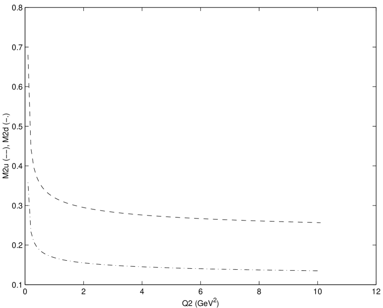
Figure 2: Scale dependence of the proton momentum fraction $M_{2}^{q_{val}}$ calculated with the Isgur-Karl model.

The ensuing $M_{2}$ momenta for the u and d quarks in the proton are reported in Fig. 2. The scale dependence for the single momenta is quite smooth apart from the low $Q^{2}$-values.

2) The hypercentral Constituent Quark Model (hCQM) is based on a Coulomb-like potential plus a linear confining potential to which a OGE-hyperfine interaction is added. The difference with the IK model is mainly in the spatial wave functions which are not gaussians, but are more spread out and are obtained by numerical solution of the $3-$quark wave equation. Moreover, the nucleon state is written as a superposition of five SU(6)- configurations:

$$|N\rangle~{}=~{}a_{S}|56,0^{+}\rangle~{}+~{}a_{S}^{\prime}|56^{\prime},0^{+}\rangle~{}+~{}a_{S}^{\prime\prime}|56^{\prime\prime},0^{+}\rangle~{}+~{}a_{M}|70,0^{+}\rangle~{}+~{}a_{D}|70,2^{+}\rangle~{}$$ (15)

with $a_{S}=0.9997,a_{S}^{\prime}=0.0217,a_{S}^{\prime\prime}=0.0041,a_{M}=0.0038,a_{D}=-0.0012$. Without the OGE-SU(6) breaking term $a_{S}^{\prime}=a_{S}^{\prime\prime}=a_{M}=a_{D}=0$. The resulting momentum density distribution contains higher momentum components in comparison with the h.o one.

2_bis) The SU(6) invariant hamiltonian is left unchanged, while the SU(6)-breaking mechanism is provided by a spin- and isospin-dependent interaction [26]. Here also the content of high momentum component is greater than in the h.o. case.

3) In the model proposed by Iachello et al.[6] the hamiltonian consists of a part corresponding to the vibration and rotation of a top to which a Gürsey-Radicati spin and isospin dependent term is added. The Gürsey-Radicati term is diagonal with respect to the SU(6)-configurations, so it splits but does not mix the $SU(6)-$configurations. An $SU(6)$-breaking mechanism is implemented in a phenomenological way considering different $u$ and $d$ charge distributions [27], which correspond to different $u$ and $d$ effective charge radii. In this way the nucleon elastic form factors are obtained folding the top form factors with the $u$ and $d$ charge distributions (assumed to be exponential-like) and the results have a dipole behaviour.

Also in this case the momentum density distribution contains high momentum components and one can imagine that this will strongly influence the results.

The unpolarized valence quark distributions are given by [28]

$$n_{q}(|\mbox{\bf k}|)=~{}\frac{8}{\pi^{2}~{}a_{q}^{3}}\frac{{\mathcal{N}}_{q}}{\left(1+\frac{\mbox{\bf k}^{2}}{a_{q}^{2}}\right)^{4}}$$ (16)

where:

$${\mathcal{N}}_{u}=2\hskip 56.9055pt{\mathcal{N}}_{d}=1$$

$$a_{u}^{-1}=0.258~{}\mbox{fm}\hskip 56.9055pta_{d}^{-1}=0.285~{}\mbox{fm}.$$

The validity of Eq. (1) for the model 2_bis is analyzed in Fig. 3. The two members are equal within 0.2 %, although the $\kappa$-ratio differs by about 7 % from the experimental value ($\sim-0.937$).

Similar results, reported in Table I, hold for the other models, with the exception of the U(7) model, where the $\kappa$-value is correctly reproduced by construction, while the equation is violated up to a few percent.

In order to test if this feature depends on the choice of the CQMs or is a general characteristic, we have used the analytic expression supplied by the Isgur-Karl model and tried to reproduce the experimental value of the two ratios by leaving the amplitudes $a_{S}^{\prime}$,$a_{M}$ and $a_{D}$ free. One can also vary the h.o. constant $\alpha$, with $\alpha^{-1}$ being a measure of the confinement radius. The $Q^{2}$-behaviour of the I.K. model is unrealistic because of the gauss-factors, however also in this case the ratio is quite scale independent. The procedure of fitting the amplitudes corresponds to introduce implicitly quite different hamiltonians. The anomalous magnetic moments have the following expressions:

$$\kappa_{p} = 2(1-a_{M}^{2})-4a_{D}^{2}$$

$$\kappa_{n} = -2(1-a_{M}^{2})+3/2~{}a_{D}^{2}~{}.$$ (17)

If one adopts a model where the only SU(6) breaking comes from the $a_{M}$, it is immediately seen from equation (17) that the $\kappa$-ratio is exactely equal to -1, like in the SU(6) limit. The crucial quantity seems then to be the $a_{D}$ amplitude. Assuming that the D-wave amplitude is the only SU(6)-breaking term (D-model), we have that:

$$\frac{2a_{S}^{2}-a_{D}^{2}}{-2a_{S}^{2}-1/2~{}a_{D}^{2}}=-0.937$$

if $a_{S}=0.955$ and $a_{D}=0.295$. Calculating the rhs of Eq. (1), which we refer as R in the following, with these two values of the parameter and varying $\alpha$ in a quite large interval, the best value obtainable is $R=0.9988$, with $\alpha=2.1~{}fm^{-1}$, differing by about 7% from the $\kappa$-ratio. Finally, leaving completely free the amplitudes $a_{S}^{\prime}$, $a_{M}$ and $a_{D}$ in order to fit the $\kappa$-ratio and R separately, the resulting amplitudes turn out to be complex.

Therefore, the proposed Equation (1) seems to be valid (up to few percent) for all Constituent Quark Models provided that the SU(6)-violation is not too strong, but both values are quite far from the experimental value of the $\kappa$-ratio of $-0.937$. If one tries to force the SU(6)-violation to reproduce the experimental value, one is apparently faced with too strong constraints coming from the CQM itself. This is a possible indication that the degrees of freedom introduced in the current CQM may be inadequate since one has to take into account pion cloud effects [29, 30].

4 Discussion and Conclusions

The relation Eq. (1) between the ratio of the proton and neutron anomalous magnetic moments and the momentum fractions carried by valence quarks, $M_{2}^{q_{val}}$, is exactly verified in the SU(6)-invariant limit, where both are equal to -1.

In the currently used Constituent Quark Models, SU(6) violations are introduced in different ways (One-Gluon-Exchange interaction, spin and/or isospin dependent terms, Gürsey-Radicati mass formula, One-Boson-Exchange …). Such SU(6) violation is necessary in order to bring the anomalous proton and neutron magnetic moments closer to the experimental values or to reproduce important features of the spectrum, such as the N-$\Delta$ mass difference.
In all the models we have considered in this paper (see Table I) the equality of Eq.(1) holds within a few percent accuracy. This agreement is based on what all the CQMs have in common: the effective degrees of freedom of the three constituent quarks and the underlying SU(6) symmetry.
On the other hand, the experimental value of the ratio is not reproduced by CQMs, at variance with the calculations based on phenomenological parton distributions reported in Fig. 1. This means that the SU(6)-breaking mechanism contained in the phenomenological partonic distributions does not correspond to the SU(6) breaking mechanism implemented in the CQMs we have analyzed.
The quark densities as given in Eqs. (13,14) are evaluated in the rest frame, as we are using non-relativistic wavefunctions in this paper. It is clear that in this way, relativistic boost effects are not included. Further work to quantify these relativistic boost effects is underway, even if we do not expect them to change in any important way our conclusion for the ratio of Eq. (1).
To conclude, it seems that all CQMs are too strongly constrained by the presence of the standard degrees of freedom corresponding to three constituent quarks. Therefore additional degrees of freedom should be introduced, in particular quark antiquark pairs and/or gluons and the discussed equation of Ref. [8], being sensitive to the SU(6)-breaking mechanism, will provide a useful tool for testing the new models.

Figure 1: Scale dependence of the rhs of Eq. (1) for various phenomenological forward parton distributions as indicated on the curves. Dotted curves : MRST parton distributions (MRST98 NLO [19], MRST01 NLO [16], MRST01 NNLO [17]). Dashed curves : CTEQ parton distributions (CTEQ5M NLO [20], CTEQ6M NLO [18]). Dashed-dotted curve : GRV98 NLO(${\overline{\mathrm{MS}}}$) [21]. Also shown is the lhs of Eq. (1), i.e. the experimental value for $\kappa^{p}/\kappa^{n}$ (constant solid curve).

Figure 3: The R-ratio for the HCQM with isospin dependence compared with the $\kappa$-ratio calculated with the same model and with the experimental value of the $\kappa$-ratio .

	I.K.	HCQM + OGE	HCQM + Isospin	U7
Model prediction for $\frac{\kappa_{p}}{\kappa_{n}}$	-1.0	-1.0	-1.0	-0.9372
R-ratio at $Q^{2}=0.5~{}\mbox{GeV}^{2}$	-1.0098	-1.0030	-0.9983	-0.9881
R-ratio at $Q^{2}=5.0~{}\mbox{GeV}^{2}$	-1.0098	-1.0030	-0.9983	-0.9881
R-ratio at $Q^{2}=10.0~{}\mbox{GeV}^{2}$	-1.0098	-1.0030	-0.9983	-0.9881

Table 1: Different CQM predictions for the R-ratio and for the $\kappa$-ratio $~{}\kappa^{p}/\kappa^{n}$

References

- [1] N. Isgur and G. Karl, Phys. Rev. D18, 4187 (1978); D19, 2653 (1979); D20, 1191 (1979); S. Godfrey and N. Isgur, Phys. Rev. D32, 189 (1985).
- [2] S. Capstick and N. Isgur, Phys. Rev. D 34,2809 (1986).
- [3] M. Ferraris, M. M. Giannini, M. Pizzo, E. Santopinto and L. Tiator, Phys. Lett. B 364, 231 (1995); M. M. Giannini, E. Santopinto and A. Vassallo, Nucl. Phys. A 699, 308 (2002).
- [4] M. Aiello, M. M. Giannini and E. Santopinto, J. Phys. G 24, 753 (1998).
- [5] L. Ya. Glozman and D.O. Riska, Phys. Rep. C268, 263 (1996).
- [6] R. Bijker, F. Iachello and A. Leviatan, Ann. Phys. (N.Y.) 236, 69 ( 1994).
- [7] L. Ya. Glozman, Z. Papp, W. Plessas, K. Varga, R. F. Wagenbrunn, Phys. Rev. C57, 3406 (1998); L. Ya. Glozman, W. Plessas, K. Varga, R. F. Wagenbrunn, Phys. Rev. D58, 094030 (1998).
- [8] K. Goeke, V. Polyakov and M. Vanderhaeghen, Prog. Part. Nucl. Phys. 47 (2001) 401.
-
[9]
A.J. Buras, Rev. Mod. Phys. 50 (1980) 199;
R.G. Roberts, The Structure of the Proton (Cambridge Univ. Press, Cambridge, (1990). -
[10]
A.D. Martin, W.J. Stirling, R.G. Roberts, Ral Report 94-055; Ral Report 95-021;
CTEQ Collab., H.L. Lau et al., Phys. Rev. D 51 (1995) 4763. -
[11]
M. Glueck and E. Reya, Phys. Rev. D 14 (1976) 3024;
E. Reya, Phys. Rep. 69 (1981) 195;
M. Glueck, E. Reya and A. Vogt, Z. Phys. C 48 (1990) 471;C 53 (1992) 127; C 67 (1995) 433. - [12] G. Parisi and R. Petronzio, Phys. Lett. B 62 (1976) 331.
- [13] R.L. Jaffe and G.C. Ross, Phys. Lett. B 93 (1980) 313.
- [14] M. Traini, V. Vento, A. Mair and A. Zambarda, Nucl. Phys. A 614 (1997) 472.
- [15] A. Mair, M. Traini, Nucl. Phys. A 624, 564 (1997); A. Mair, M. Traini, Nucl. Phys. A 628, 296 (1998).
- [16] A.D. Martin, R.G. Roberts, W.J. Stirling, and R.S. Thorne, Eur. Phys. J. C 23, 73 (2002).
- [17] A.D. Martin, R.G. Roberts, W.J. Stirling, and R.S. Thorne, Phys. Lett. B 531, 216 (2002).
- [18] J. Pumplin, D.R. Stump, J. Huston, H.L. Lai, P. Nadolsky, and W.K. Tung, hep-ph/0201195.
- [19] A.D. Martin, R.G. Roberts, W.J. Stirling, and R.S. Thorne, Eur. Phys. J. C 4, 463 (1998).
- [20] H.L. Lai, et al., Eur. Phys. J. C 12, 375 (2000).
- [21] M. Glück, E. Reya, and A. Vogt, Eur. Phys. J. C 5, 461 (1998).
- [22] M. Glück, E. Reya and A. Vogt, Z. Phys. C 53 (1992) 127.
- [23] T. Weigl and W. Melnitchouk, Nucl. Phys. B465 (1996) 267.
- [24] L. Heller, in “Quarks and Nuclear Forces”, eds. D. C. Vries and B. Zeitnitz, Springer Tracts in Modern Physics 100, 145 (1982); M. Campostrini, K. Moriarty, C. Rebbi, Phys. Rev. D 36, 3450, (1987); G. S. Bali, Phys. Rept. 343, 1 (2001).
- [25] M. D. Sanctis, M. M. Giannini, L. Repetto and E. Santopinto, Phys. Rev. C 62, 025208 (2000).
- [26] M. M. Giannini, E. Santopinto and A. Vassallo, Eur. Phys. J. A 12, 447 (2001).
- [27] R. Bijker, F. Iachello, A. Leviatan, Phys.Rev. C 54 1935 (1996).
- [28] F. Iachello, Private comunication.
- [29] H. Dahiya and M. Gupta, Phys. Rev. D 66, 051501 (2002).
- [30] I. C. Cloet, D. B. Leinweber and A. W. Thomas, Phys. Rev. C 65, 062201 (2002).