Calculated Corrections to Superallowed Fermi Beta Decay: New Evaluation of the Nuclear-Structure-Dependent Terms

Abstract

The measured $ft$-values for superallowed $0^{+}\rightarrow 0^{+}$ nuclear $\beta$-decay can be used to obtain the value of the vector coupling constant and thus to test the unitarity of the Cabibbo-Kobayashi-Maskawa matrix. An essential requirement for this test is accurate calculations for the radiative and isospin symmetry-breaking corrections that must be applied to the experimental data. We present a new and consistent set of calculations for the nuclear-structure-dependent components of these corrections. These new results do not alter the current status of the unitarity test – it still fails by more than two standard deviations – but they provide calculated corrections for eleven new superallowed transitions that are likely to become accessible to precise measurements in the future. The reliability of all calculated corrections is explored and an experimental method indicated by which the structure-dependent corrections can be tested and, if necessary, improved.

I Introduction

Superallowed $0^{+}\rightarrow 0^{+}$ nuclear $\beta$-decay depends uniquely on the vector part of the weak interaction. When it occurs between $T=1$ analog states, a precise measurement of the transition $ft$-value can be used to determine $G_{\mbox{\tiny V}}$, the vector coupling constant. This result, in turn, yields $V_{ud}$, the up-down element of the Cabibbo-Kobayashi-Maskawa (CKM) matrix. At this time, it is the key ingredient in one of the most exacting tests available of the unitarity of the CKM matrix, a fundamental pillar of the minimal Standard Model.

Currently, there is a substantial body of precise $ft$-values determined for such transitions and the experimental results are robust, most input data having been obtained from several independent and consistent measurements TH98 ; Ha90 . In all, $ft$-values have been determined for nine $0^{+}\rightarrow 0^{+}$ transitions to a precision of $\sim 0.1\%$ or better. The decay parents – ¹⁰C, ¹⁴O,^26mAl,³⁴Cl,^38mK,⁴²Sc,⁴⁶V,⁵⁰Mn and ⁵⁴Co – span a wide range of nuclear masses; nevertheless, as anticipated by the Conserved Vector Current hypothesis, CVC, all nine yield consistent values for $G_{\mbox{\tiny V}}$, from which a value of

$$V_{ud}=0.9740\pm 0.0005$$ (1)

is derived. The unitarity test of the CKM matrix, made possible by this precise value of $V_{ud}$, fails by more than two standard deviations TH98 : viz.

$$V_{ud}^{2}+V_{us}^{2}+V_{ub}^{2}=0.9968\pm 0.0014.$$ (2)

In obtaining this result, we have used the Particle Data Group’s PDG00 recommended values for the much smaller matrix elements, $V_{us}$ and $V_{ub}$. Although this deviation from unitarity is not completely definitive statistically, it is also supported by recent, less precise results from neutron decay Ab02 . If the precision of this test can be improved and it continues to indicate non-unitarity, then the consequences for the Standard Model would be far-reaching.

The potential impact of definitive non-unitarity has led to considerable recent activity, both experimental and theoretical, in the study of superallowed $0^{+}\rightarrow 0^{+}$ transitions, with special attention being focussed on the small correction terms that must be applied to the experimental $ft$-values in order to extract $G_{\mbox{\tiny V}}$. Specifically, $G_{\mbox{\tiny V}}$ is obtained from each $ft$-value via the relationship TH98

$${\cal F}t\equiv ft(1+\delta_{R})(1-\delta_{C})=\frac{K}{2G_{\mbox{\tiny V}}^{2}(1+\Delta_{\mbox{\tiny R}}^{\mbox{\tiny V}})},$$ (3)

with

$$K/(\hbar c)^{6} = 2\pi^{3}\hbar\ln 2/(m_{e}c^{2})^{5}$$ (4)

$$= (8120.271\pm 0.012)\times 10^{-10}{\rm GeV}^{-4}{\rm s},$$

where $f$ is the statistical rate function, $t$ is the partial half-life for the transition, $\delta_{C}$ is the isospin-symmetry-breaking correction, $\delta_{R}$ is the transition-dependent part of the radiative correction and $\Delta_{\mbox{\tiny R}}^{\mbox{\tiny V}}$ is the transition-independent part. Here we have also defined ${\cal F}t$ as the “corrected” $ft$-value.

It is now convenient to separate the radiative correction into two terms:

$$\delta_{R}=\delta_{R}^{\prime}+\delta_{NS}$$ (5)

where the first term, $\delta_{R}^{\prime}$, is a function of the electron’s energy and the charge of the daughter nucleus, $Z$; it therefore depends on the particular nuclear decay, but is independent of nuclear structure. The second term, $\delta_{NS}$, is discussed more fully in Sec. II.2 but its evaluation, like $\delta_{C}$, depends on the details of nuclear structure. To emphasize the different sensitivities of the correction terms we re-write the expression for ${\cal F}t$ as

$${\cal F}t\equiv ft(1+\delta_{R}^{\prime})(1+\delta_{NS}-\delta_{C})$$ (6)

where the first correction in brackets is independent of nuclear structure, while the second incorporates the structure-dependent terms. The term $\delta_{R}^{\prime}$ has been calculated from standard QED, and is currently evaluated to order $Z\alpha^{2}$ and estimated in order $Z^{2}\alpha^{3}$ Si87 ; JR87 ; its values are around 1.4% and can be considered very reliable. The structure-dependent terms, $\delta_{NS}$ and $\delta_{C}$, have also been calculated in the past but at various times over three decades and with a variety of different nuclear models. Their uncertainties are larger. This paper specifically addresses these correction terms with a view to reducing their uncertainties.

Though depending on the nuclear shell-model, calculations for $\delta_{NS}$ and $\delta_{C}$ have been carefully linked to other related observables such as the neutron and proton binding energies, the $b$- and $c$-coefficients in the Isobaric Multiplet Mass Equation (IMME), and the non-analog $0^{+}\rightarrow 0^{+}$ transition rates (see, for example, OB85 ; Ha94 ; THH77 ). Given this linking to observables and the more general success of the shell model in this mass region, calculations of $\delta_{NS}$ and $\delta_{C}$ should also be rather reliable. Nevertheless, conservative uncertainties have been applied – they are of order 0.1% (i.e. $\sim 10\%$ of their own value) – and these become major contributors to the overall uncertainty on the unitarity test. To illustrate: the uncertainty obtained for $V_{ud}$ in Eq.(1)is $\pm 0.0005$; the contributions to this uncertainty are 0.0001 from experiment, 0.0001 from $\delta_{R}^{\prime}$, 0.0003 from $\delta_{C}-\delta_{NS}$, and 0.0004 from $\Delta_{\mbox{\tiny R}}^{\mbox{\tiny V}}$. If the unitarity test is to be sharpened, then the most pressing objective must be to reduce the uncertainties on $\Delta_{\mbox{\tiny R}}^{\mbox{\tiny V}}$ and ($\delta_{C}-\delta_{NS}$). The latter is clearly the most important area where nuclear physics can play an critical role. There is considerable activity, both experimental and theoretical, now underway in probing these nuclear-structure-dependent corrections with a view to reducing the uncertainty that they introduce into the unitarity test.

Since the goal of experiments will generally be to test and constrain the calculated structure-dependent corrections, an important first step is to have a set of consistent calculations that apply both to the nine well-known transitions already used for the unitarity test and to possible new cases yet to be studied. In what follows, we present new calculations of $\delta_{C}$ and $\delta_{NS}$, in which consistent model spaces and approximations have been used for both correction terms and for a large repertoire of superallowed transitions, new and old. These will provide a consistent standard for future experimental comparison.

II Theoretical corrections to superallowed decays

As described in the introduction, there are four theoretical correction terms involved in extracting $V_{ud}$ from experimental $ft$-values: the radiative corrections that are independent of nuclear structure ($\delta_{R}^{\prime}$ and $\Delta_{\mbox{\tiny R}}^{\mbox{\tiny V}}$), the nuclear-structure-dependent radiative correction ($\delta_{NS}$) and the isospin-symmetry-breaking correction ($\delta_{C}$). Though we will later present new calculations of the last two, in this section we present an overview of all four terms. This overview is placed in the context of a unitarity test that has failed by more than two standard deviations. In particular, we assess whether the failure to meet unitarity can be removed by plausible adjustments in these calculated corrections. What changes would it take to restore unitarity? For example, $\delta_{R}^{\prime}$, would have to be shifted downwards by 0.3% (i.e.  as much as one-quarter of its current value) for all nine currently well-measured nuclear transitions; or ($\delta_{C}-\delta_{NS}$) would have to be shifted upwards by 0.3% (over one-half their value), for all nine cases; or some combination of the two. We will argue that such shifts are very improbable.

II.1 Radiative corrections independent of nuclear structure

The radiative correction comprises a transition-dependent term, $\delta_{R}$, and a transition-independent term, $\Delta_{\mbox{\tiny R}}^{\mbox{\tiny V}}$. The transition-dependent term is further divided into $\delta_{R}^{\prime}$, which does not depend on nuclear structure, and $\delta_{NS}$, which is structure dependent. We consider first the structure-independent terms, which are written:

$$\delta_{R}^{\prime} = \frac{\alpha}{2\pi}\left[\overline{g}(E_{m})+\delta_{2}+\delta_{3}\right],$$ (7)

$$\Delta_{\mbox{\tiny R}}^{\mbox{\tiny V}} = \frac{\alpha}{2\pi}\left[4\ln(m_{\mbox{\tiny Z}}/m_{p})+\ln(m_{p}/m_{\mbox{\tiny A}})+2C_{\rm Born}\right]+\cdots,$$

where the ellipses represent further small terms of order 0.1%. In these equations, $E_{m}$ is the maximum electron energy in beta decay, $m_{\mbox{\tiny Z}}$ the $Z$-boson mass, $m_{p}$ the proton mass, $m_{\mbox{\tiny A}}$ the $a_{1}$-meson mass, and $\delta_{2}$ and $\delta_{3}$ the order-$Z\alpha^{2}$ and -$Z^{2}\alpha^{3}$ contributions respectively. The function $g(E_{e},E_{m})$, which depends on the electron energy, was first defined by Sirlin Si67 as part of the order-$\alpha$ universal photonic contribution arising from the weak vector current; it is here averaged over the electron spectrum to give $\overline{g}(E_{m})$. Finally, the term $C_{\rm Born}$ comes from the order-$\alpha$ axial-vector photonic contributions.

Calculated values for all three components of $\delta_{R}^{\prime}$ are given in Table 1. There have been two independent calculations Si87 ; JR87 of both $\delta_{2}$ and $\delta_{3}$; they are completely consistent with one another if proper account is taken of finite-size effects in the nuclear charge distribution. The values listed in Table 1 are our recalculations Ha90 using the formulas of Sirlin Si87 but incorporating a Fermi charge-density distribution for the nucleus. Note that we have followed Sirlin in assigning an uncertainty equal to $(\alpha/2\pi)\delta_{3}$ as an estimate of the error made in stopping the calculation at that order.

Table 1: Calculated nucleus-dependent radiative correction, $\delta_{R}$, in percent units, and the component contributions as identified in Eq. (7).

	$\frac{\alpha}{2\pi}\overline{g}(E_{m})$	$\frac{\alpha}{2\pi}\delta_{2}$	$\frac{\alpha}{2\pi}\delta_{3}$	$\delta_{R}^{\prime}$
$T_{z}=-1$:
10C	1.468	0.182	0.005	1.65(1)
14O	1.286	0.227	0.008	1.52(1)
18Ne	1.204	0.268	0.013	1.48(1)
22Mg	1.121	0.305	0.018	1.44(2)
26Si	1.055	0.338	0.024	1.42(2)
30S	1.005	0.363	0.030	1.40(3)
34Ar	0.963	0.392	0.037	1.39(4)
38Ca	0.928	0.417	0.044	1.39(4)
42Ti	0.906	0.449	0.053	1.41(5)
$T_{z}=0$:
26mAl	1.110	0.325	0.021	1.46(2)
34Cl	1.002	0.388	0.034	1.42(3)
38mK	0.964	0.413	0.041	1.42(4)
42Sc	0.939	0.448	0.049	1.44(5)
46V	0.903	0.468	0.057	1.43(6)
50Mn	0.873	0.494	0.065	1.43(7)
54Co	0.843	0.507	0.073	1.42(7)
62Ga	0.805	0.567	0.091	1.46(9)
66As	0.791	0.589	0.100	1.48(10)
70Br	0.777	0.609	0.110	1.50(11)
74Rb	0.763	0.627	0.120	1.51(12)

To assess the changes in $\delta_{R}^{\prime}$ that would be required in order to restore unitarity, it is helpful to rewrite Eq. (7) in terms of the typical values taken by its components: viz.

$$\delta_{R}^{\prime}\simeq 1.00+0.40+0.05\%,$$ (8)

If the failure to obtain unitarity in the CKM matrix with $V_{ud}$ from nuclear beta decay is due to the value of this term alone, then $\delta_{R}^{\prime}$ must be reduced to 1.1%. This is not likely. The leading term, 1.00%, involves standard QED and is well verified. The order-$Z\alpha^{2}$ term, 0.40%, while less secure has been calculated twice Si87 ; JR87 independently, with results in accord.

Taking a similar approach for the nucleus-independent radiative correction, we write

$$\Delta_{\mbox{\tiny R}}^{\mbox{\tiny V}}=2.12-0.03+0.20+0.1\%~{}~{}\simeq~{}~{}2.4\%,$$ (9)

of which the first term, the leading logarithm, is unambiguous. Again, to achieve unitarity of the CKM matrix, $\Delta_{\mbox{\tiny R}}^{\mbox{\tiny V}}$ would have to be reduced to 2.1%: i.e.  all terms other than the leading logarithm must sum to zero. This also seems unlikely. The adopted value of the nucleus-independent radiative correction has been set at Si94

$$\Delta_{\mbox{\tiny R}}^{\mbox{\tiny V}}=(2.40\pm 0.08)\%.$$ (10)

Note this value differs slightly (but within errors) from an earlier value MS86 because of the decision by Sirlin Si94 to centre the cut-off parameter $m_{\mbox{\tiny A}}$, where $(m_{a_{1}}/2)\leq m_{\mbox{\tiny A}}\leq 2m_{a_{1}}$, exactly at the $a_{1}$-meson mass when evaluating the axial contribution to the radiative-correction loop graph. This range of possible values for $m_{\mbox{\tiny A}}$ is the dominant contributor to the error in Eq. (10).

II.2 The $\delta_{NS}$ correction

The nuclear-structure-dependent part of the radiative correction is denoted $\delta_{NS}$. Although for the superallowed transition we are discussing a purely vector interaction between spin $0^{+}$ states, the axial-vector interaction does play a role in the radiative corrections. An axial-vector interaction may flip a nucleon spin and then be followed by an electromagnetic interaction that flips it back again. This axial contribution, denoted $C$, can be further divided into two terms depending whether the weak and electromagnetic interactions occur on the same nucleon or on two separate nucleons:

$$C = C_{{\rm Born}}+C_{NS},$$

$$\delta_{NS} = \frac{\alpha}{\pi}C_{NS}.$$ (11)

Here $C_{{\rm Born}}$ refers to the Born graph in which the axial-vector and electromagnetic interactions occur on the same nucleon. This term is universal – i.e.  the same in all nuclei – so it is not included in $\delta_{NS}$ but is placed in the nucleus-independent radiative correction $\Delta_{\mbox{\tiny R}}^{\mbox{\tiny V}}$, see Eq. (7). The term, $C_{NS}$, refers to the case when the axial-vector and electromagnetic interactions occur on different nucleons. The calculation of this term depends on the details of nuclear structure.

In the earliest calculations of $\delta_{NS}$ JR90 ; BBJR92 ; To92 , the axial-vector and electromagnetic vertices were evaluated with free-nucleon coupling constants. Yet there is ample evidence in nuclear physics that coupling constants for spin-flip processes are quenched in the nuclear medium. Subsequently, Towner To94 revised his earlier results To92 using quenching factors that had been obtained previously To87 ; ASBH87 ; BW83 from studies of weak and electromagnetic transitions in nuclei throughout the region $10\leq A\leq 54$. These quenching factors depend weakly on both mass and shell-model orbital.

Table 2: Shell-model calculations of the nuclear-structure dependent component of the radiative correction, $\delta_{NS}$. The four components that are summed to give $C_{NS}$ characterize the four electromagnetic couplings: os = orbital isoscalar, ss = spin isoscalar, ov = orbital isovector, and sv = spin isovector.

Parent	Unquenched	Quenched $C_{NS}$					$(q-1)\times$	$\delta_{NS}(\%)$
nucleus	$C_{NS}$	os	ss	ov	sv	total	$C_{{\rm Born}}({\rm free})$	Quenched	Adopted
$T_{z}=-1$:
10C	$-1.669$	$0.002$	$-0.283$	$-0.002$	$-1.065$	$-1.348$	$-0.188$	$-0.357$	$-0.360(35)$
14O	$-1.360$	$-0.008$	$-0.341$	$0.082$	$-0.782$	$-1.049$	$-0.221$	$-0.295$	$-0.250(50)$
18Ne	$-1.531$	$-0.011$	$-0.249$	$-0.119$	$-0.812$	$-1.191$	$-0.210$	$-0.325$	$-0.290(35)$
22Mg	$-1.046$	$-0.009$	$-0.222$	$-0.067$	$-0.497$	$-0.796$	$-0.226$	$-0.237$	$-0.240(20)$
26Si	$-0.986$	$-0.007$	$-0.224$	$-0.086$	$-0.424$	$-0.741$	$-0.242$	$-0.228$	$-0.230(20)$
30S	$-0.800$	$0.002$	$-0.287$	$0.020$	$-0.300$	$-0.566$	$-0.257$	$-0.191$	$-0.190(15)$
34Ar	$-0.770$	$0.014$	$-0.322$	$0.061$	$-0.272$	$-0.519$	$-0.273$	$-0.184$	$-0.185(15)$
38Ca	$-0.693$	$0.041$	$-0.358$	$0.091$	$-0.214$	$-0.440$	$-0.288$	$-0.169$	$-0.180(15)$
42Ti	$-1.011$	$-0.016$	$-0.181$	$-0.225$	$-0.354$	$-0.776$	$-0.256$	$-0.240$	$-0.240(20)$
$T_{z}=0$:
26mAl	$0.352$	$-0.007$	$-0.224$	$0.086$	$0.424$	$0.279$	$-0.242$	$0.009$	$0.009(20)$
34Cl	$-0.135$	$0.015$	$-0.333$	$-0.064$	$0.280$	$-0.101$	$-0.273$	$-0.087$	$-0.085(15)$
38mK	$-0.276$	$0.042$	$-0.363$	$-0.093$	$0.216$	$-0.198$	$-0.288$	$-0.113$	$-0.100(15)$
42Sc	$0.472$	$-0.016$	$-0.182$	$0.228$	$0.358$	$0.389$	$-0.256$	$0.031$	$0.030(20)$
46V	$0.101$	$-0.004$	$-0.197$	$0.099$	$0.198$	$0.096$	$-0.263$	$-0.039$	$-0.040(7)$
50Mn	$0.054$	$-0.009$	$-0.184$	$0.104$	$0.152$	$0.063$	$-0.270$	$-0.048$	$-0.042(7)$
54Co	$0.161$	$-0.013$	$-0.180$	$0.133$	$0.203$	$0.144$	$-0.277$	$-0.031$	$-0.029(7)$
62Ga	$0.172$	$0.005$	$-0.289$	$-0.058$	$0.445$	$0.103$	$-0.289$	$-0.043$	$-0.040(20)$
66As	$0.124$	$0.006$	$-0.291$	$-0.070$	$0.421$	$0.066$	$-0.295$	$-0.053$	$-0.050(20)$
70Br	$0.077$	$0.009$	$-0.295$	$-0.083$	$0.401$	$0.032$	$-0.301$	$-0.063$	$-0.060(20)$
74Rb	$0.155$	$0.009$	$-0.261$	$0.006$	$0.353$	$0.106$	$-0.306$	$-0.046$	$-0.065(20)$

There is a further consideration. The presence of quenching also breaks the universality of the Born term, $C_{{\rm Born}}$. Writing the evaluation of $C_{{\rm Born}}$ with free-nucleon coupling constants as $C_{{\rm Born}}({\rm free})$, then $C_{{\rm Born}}({\rm quenched})$ can be written:

$$C_{{\rm Born}}({\rm quenched}) = qC_{{\rm Born}}({\rm free})$$

$$= C_{{\rm Born}}({\rm free})+(q-1)C_{{\rm Born}}({\rm free}),$$

where $q$ is the factor by which the product of the weak and electromagnetic coupling constants is reduced in the medium relative to its free-nucleon value. The first term in Eq. (II.2) remains universal, while the second term is now part of the nuclear-structure dependence of the radiative correction. Thus $\delta_{NS}$ is written

$$\delta_{NS}=\frac{\alpha}{\pi}\left\{C_{NS}({\rm quenched})+(q-1)C_{{\rm Born}}({\rm free})\right\}.$$ (13)

We have calculated the $\delta_{NS}$ correction for a wide range of nuclei with $0^{+}$ ($T=1$) ground or isomeric states that decay by superallowed $\beta$-emission; we used the shell model with effective interactions as described in Appendix A. Results for both quenched and unquenched coupling constants are given in Table 2. All but the last column in that table give the results from one particular calculation for each parent nuclide. (In most cases, two or three independent calculations were performed for a single parent, each with a different shell-model Hamiltonian.) The last column lists the values we adopt for $\delta_{NS}$: these values result from our assessment of the quenched results from all calculations made for each decay – not just the ones shown in the previous columns – with uncertainties chosen to encompass the spread in the results from those calculations.

Extra details are also given in columns 3-6 of the table for the quenched calculation since this is the version that we ultimately use in evaluating $V_{ud}$. With two-body operators there are two types of contributions: those in which both interacting nucleons are in the valence model space, and those in which one nucleon is in the valence space and one is in the closed-shells core. In the latter case a sum is required over all the core nucleons. The isospin structure of the operator is interesting to note: the weak interaction contribution is isovector, while the electromagnetic contribution is isoscalar or isovector. The combined operator therefore is either isovector or isotensor. (An isoscalar combination is just proportional to the unit operator in isospin space and does not induce a Fermi transition.) Both the valence nucleons and those in the core contribute to the result for isovector operators, only the valence nucleons contribute to the isotensor operators.

In Table 2 we show contributions to $C_{NS}$ from the various components of the electromagnetic interaction: orbital isoscalar (os), spin isoscalar (ss), orbital isovector (ov) and spin isovector (sv). Note that the spin contributions are larger than the orbital contributions. Further, and more interesting, the isoscalar and isovector contributions are in phase when the decaying nucleus has $T_{z}=-1$ and out of phase when the decaying nucleus has $T_{z}=0$. This indicates that much larger corrections are obtained in the $T_{z}=-1$ series than in the $T_{z}=0$ series. If one looks at mirror transitions, this effect alone contributes between $0.1\%$ to $0.3\%$ to a mirror asymmetry in the $ft$-values. Since current experiments aim at $0.1\%$ accuracy, this effect might just be at the edge of detectability.

II.3 Isospin symmetry-breaking corrections

Turning, next, to the isospin-symmetry breaking correction, $\delta_{C}$, it too can be separated into two components:

$$\delta_{C}=\delta_{C1}+\delta_{C2}.$$ (14)

The first term, $\delta_{C1}$, arises from Coulomb and charge-dependent nuclear interactions that induce configuration mixing among the $0^{+}$ state wave functions in both the parent and daughter nuclei. Being charge dependent, this mixing serves to break isospin symmetry between the analog parent and daughter states of the superallowed transition. The second term, $\delta_{C2}$, is due to small differences in the single-particle neutron and proton radial wave functions, which cause the radial overlap integral of the parent and daughter nucleus to be less than unity. Strictly speaking, these two aspects of the calculation of $\delta_{C}$ cannot be separated, but in all but one calculation to date (including those reported here) this division has been made. (The exception is the $(0+2+4)\hbar\omega$ large-basis shell-model calculation of Navrátil et al.NBO97 for the lightest superallowed emitter, ¹⁰C.) This division is akin to the division made in setting up a shell-model calculation, where the configuration space is divided into a small, tractible valence space and a remaining excluded space. Then $\delta_{C1}$ arises from the charge-dependent mixing within the valence space, while $\delta_{C2}$ represents the consequence of mixing between configurations in the valence space with those in the excluded space; this consequence being manifested by a change in the single-particle radial wave function of the valence nucleons.

II.3.1 The $\delta_{C1}$ correction

If, in a shell-model calculation, the effective interaction is isospin invariant, then the wave functions for the parent and daughter analogue states are identical, and the square of the Fermi matrix element between them (for isospin $T=1$ states) is exactly $|M_{F}|^{2}=2$. In addition, beta transitions to all other $0^{+}$ states in the daughter are strictly forbidden. However, the addition of charge-dependent terms to the effective interaction causes the breaking of analogue symmetry. Under these conditions, the Fermi matrix element departs slightly from its isospin-invariant value. We write

$$|M_{F}|^{2}=2(1-\delta_{C1}).$$ (15)

Also, with charge-dependent terms in the effective interaction, the Fermi matrix elements to other non-analogue $0^{+}$ states in the daughter are no longer exactly zero. For example, there could be small (usually less than 0.1%) branches to those excited $0^{+}$ states that are energetically accessible to beta-decay. For the first excited (non-analog) $0^{+}$ state, we can write

$$|M_{F}^{1}|^{2}=2\delta_{C1}^{1}.$$ (16)

In a model calculation in which there are only two basis states, the depletion of Fermi strength in the ground-state transition is entirely picked up by the transition to the excited non-analogue $0^{+}$ state. Thus,

$$\delta_{C1}=\delta_{C1}^{1}.$$ (17)

Further, if only two-state mixing is considered, the magnitude of $\delta_{C1}$ is inversely proportional to the square of the excitation energy of the excited $0^{+}$ state: i.e.

$$\delta_{C1}\propto\frac{1}{(\Delta E)^{2}}.$$ (18)

For our calculations, in which a large number of basis states play a role, Eqs. (17) and (18) are no longer exact. Even so, they remain approximately true and continue to be a useful guide.

Calculations of $\delta_{C1}$ turn out to be very sensitive to the details of the model calculation. This would be a very unfortunate property if we were not able to adopt certain strategies that act to reduce the model dependence considerably. Because of the variation of $\delta_{C1}$ with $(\Delta E)^{2}$ (see Eq. (18)), it is important that the isospin-independent Hamiltonian produce a good quality spectrum of $0^{+}$ states. Since this is not always possible to achieve in the shell model, especially for nuclei near to closed shells, our first strategy is to compensate for this by scaling the calculated $\delta_{C1}$ values by a factor $(\Delta E)^{2}_{{\rm theo}}/(\Delta E)^{2}_{{\rm expt}}$, the ratio of the square of the excitation energy of the first excited $0^{+}$ state in the model calculation to that known experimentally. The second strategy we adopt to reduce the model dependence was first used by Ormand and BrownOB85 ; OB89 . We constrain the charge-dependent part of the effective interaction to reproduce other charge-dependent properties of the $0^{+}$ states, namely the coefficients of the isobaric multiplet mass equation (IMME)Br98 .

Table 3: Shell-model calculations of the isospin symmetry-breaking correction, $\delta_{C1}$.

Parent	Measured IMME coefficients Br98		$E_{x}(0^{+})$	$E_{x}(0^{+})$	$\delta_{C1}(\%)$
nucleus	$b$	$c$	expt	SM	unscaled	scaled	Adopted
$T_{z}=-1$:
10C	$-1.546$	$0.362$	$6.18$	$11.05$	$0.002$	$0.007$	$0.010(10)$
14O	$-2.493$	$0.337$	$6.59$	$6.64$	$0.049$	$0.050$	$0.050(20)$
18Ne	$-3.045(1)$	$0.347(1)$	$3.63$	$3.80$	$0.212$	$0.232$	$0.230(30)$
22Mg	$-3.814(1)$	$0.315(1)$	$6.24$	$6.34$	$0.010$	$0.010$	$0.010(10)$
26Si	$-4.535(2)$	$0.302(2)$	$3.59$	$4.96$	$0.022$	$0.042$	$0.040(10)$
30S	$-5.185(2)$	$0.275(2)$	$3.79$	$3.86$	$0.186$	$0.193$	$0.195(30)$
34Ar	$-5.777(2)$	$0.286(2)$	$3.92$	$3.91$	$0.031$	$0.030$	$0.030(10)$
38Ca	$-6.328(3)$	$0.284(3)$	$3.38$	$3.21$	$0.026$	$0.023$	$0.020(10)$
42Ti	$-6.712(3)$	$0.287(3)$	$1.84$	$3.60$	$0.065$	$0.249$	$0.220(100)$
$T_{z}=0$:
26mAl	$-4.535(2)$	$0.302(2)$	$3.59$	$4.96$	$0.022$	$0.041$	$0.040(10)$
34Cl	$-5.777(2)$	$0.286(2)$	$3.92$	$3.91$	$0.103$	$0.103$	$0.105(20)$
38mK	$-6.328(3)$	$0.284(3)$	$3.38$	$3.21$	$0.099$	$0.089$	$0.100(20)$
42Sc	$-6.712(3)$	$0.287(3)$	$1.84$	$3.60$	$0.019$	$0.072$	$0.060(30)$
46V	$-7.327(10)$	$0.276(11)$	$2.61$	$3.92$	$0.043$	$0.097$	$0.095(20)$
50Mn	$-7.892(30)$	$0.259(30)$	$3.69$	$4.23$	$0.048$	$0.063$	$0.055(20)$
54Co	$-8.519(25)$	$0.276(25)$	$2.56$	$2.26$	$0.058$	$0.045$	$0.040(15)$
62Ga	$-9.463(70)$	$0.265(25)$	$2.33$	$2.26$	$0.350$	$0.330$	$0.330(40)$
66As	$-9.95(15)$	$0.262(25)$	$2.17$	$1.81$	$0.356$	$0.247$	$0.250(40)$
70Br	$-10.48(23)$	$0.260(25)$	$2.01$	$1.72$	$0.479$	$0.352$	$0.350(40)$
74Rb	$-10.82(25)$	$0.258(25)$	$0.508$	$0.523$	$0.122$	$0.129$	$0.130(60)$

There are three ways in which charge dependence enters our shell-model calculation. First, the single-particle energies of the proton orbits are shifted relative to those of the neutrons. The amount of shift is determined from the spectrum of single-particle states in the closed-shell-plus-proton versus the closed-shell-plus-neutron nucleus, where the closed shell is taken to be the nucleus used as a closed-shell core in that particular shell-model calculation. These single-particle shifts are taken from experiment and are not adjusted. Second, a two-body Coulomb interaction is added among the valence protons. The strength of this interaction is adjusted so that the $b$-coefficient of the IMME is exactly reproduced. Third, we add a charge-dependent nuclear interaction by increasing all the $T=1$ proton-neutron matrix elements by about $2\%$ relative to the neutron-neutron matrix elements. The precise amount of this increment was determined by requiring that the $c$-coefficient of the IMME be exactly reproduced.

For each of the nuclei appearing in the previous tables, we list in Table 3 the values of the corresponding measured IMME coefficients, $b$ and $c$, together with the known excitation energy, $E_{x}(0^{+})$, of the lowest excited $0^{+}$ state in their daughters. As already explained, all our shell-model calculations were adjusted to reproduce exactly the values of $b$ and $c$, and any discrepancy between the calculated and experimental values of $E_{x}(0^{+})$ was compensated for by scaling the calculated results for $\delta_{C1}$. As we did in Table 2, Columns 5-7 of in this table give the results from one particular calculation for each parent nucleus. These columns list the calculated $0^{+}$ excitation energy and $\delta_{C1}$ values, both unscaled and scaled for any $E_{x}(0^{+})$ discrepancy. Finally, the eighth column gives the $\delta_{C1}$ values we adopt. These values result from our assessment of the results of all calculations made for each decay – not just the ones shown in columns 5-7 – with uncertainties chosen to encompass the spread in the results from those calculations and to include the uncertainty in the IMME $b$- and $c$-coefficients.

For the nuclei with $A\geq 38$ there are excited (non-analogue) $0^{+}$ states in the daughter nuclei that are accessible to beta decay. Some of the Fermi transitions to these states have also been measured Ha94 ; DR85 . In Table 4 we list one set of calculated $\delta_{C1}^{1}$ values, both unscaled and scaled, along with the value of $\delta_{C1}^{1}$ we adopt based on the same assessment as that described for Table 3. As before, the assigned errors reflect both the spread among the different calculations and the uncertainties in the IMME coefficients. The measured branching ratios were then converted to $\delta_{C1}^{1}$ values (see Eq. (16)), which appear in the last column of the table. With the possible exception of the results for ⁵⁰Mn, the agreement between theory and experiment is entirely satisfactory.

Table 4: Shell-model calculations for the square of the Fermi matrix element to the first excited $0^{+}$ state, $\delta_{C1}^{1}$.

Parent	$\delta_{C1}^{1}(\%)$
nucleus	unscaled	scaled	adopted	expt
$T_{z}=0$:
38mK	0.068	0.062	0.090 (30)	$<0.28$
42Sc	0.007	0.029	0.020 (20)	$0.040(9)$
46V	0.020	0.046	0.035 (15)	$0.053(5)$
50Mn	0.038	0.049	0.045 (20)	$<0.016$
54Co	0.049	0.038	0.040 (20)	$0.035(5)$
62Ga	0.089	0.084	0.085 (20)
66As	0.027	0.019	0.020 (20)
70Br	0.095	0.070	0.070 (20)
74Rb	0.045	0.047	0.050 (30)

II.3.2 The $\delta_{C2}$ correction

The second isospin symmetry-breaking correction, $\delta_{C2}$, accounts for the difference in radial forms between the proton in the parent $\beta$-decaying nucleus and the neutron in the daughter nucleus. These radial forms are integrated together and, if there were no difference between them, the integral would just be the normalization integral of value one. The departure of the square of this overlap integral from unity corresponds to $\delta_{C2}$. There is a strong constraint on any calculation of $\delta_{C2}$: the asymptotic forms of the radial functions must be matched to the separation energies, $S_{p}$ and $S_{n}$, where $S_{p}$ is the proton separation energy in the parent nucleus and $S_{n}$ is the neutron separation energy in the daughter nucleus. These separation energies are well known and and may be found in any atomic mass table. It is the size of the difference between $S_{p}$ and $S_{n}$ and whether or not the radial wave functions have nodes that principally determine the magnitude of $\delta_{C2}$.

Our calculations of this correction follow closely the methods described in our earlier work THH77 . We use a Saxon-Woods potential defined for a nucleus of mass $A$ and charge $Z+1$ as:

$$V(r) = -V_{0}f(r)-V_{s}g(r){\bf l}.\mbox{\boldmath$\sigma$}+V_{C}(r)$$ (19)

$$~{}~{}~{}~{}~{}-V_{g}g(r)-V_{h}h(r),$$

where

$$f(r) = \left\{1+\exp\left((r-R)/a\right)\right\}^{-1},$$

$$g(r) = \left(\frac{\hbar}{m_{\pi}c}\right)^{2}\frac{1}{a_{s}r}\exp\left(\frac{r-R_{s}}{a_{s}}\right)$$

$$~{}~{}~{}~{}~{}\times\left\{1+\exp\left(\frac{r-R_{s}}{a_{s}}\right)\right\}^{-2},$$

$$h(r) = a^{2}\left(\frac{df}{dr}\right)^{2},$$

$$V_{C}(r) = Ze^{2}/r,~{}~{}~{}~{}{\rm for}~{}~{}r\geq R_{c}$$ (20)

$$= \frac{Ze^{2}}{2R_{c}}\left(3-\frac{r^{2}}{R_{c}^{2}}\right),~{}~{}~{}~{}{\rm for}~{}~{}r<R_{c},$$

with $R=r_{0}(A-1)^{1/3}$ and $R_{s}=r_{s}(A-1)^{1/3}$. Note that $g(r)$ is rendered dimensionless through the use of the pion Compton wavelength, $\left(\hbar/m_{\pi}c\right)^{2}=2$ fm². The first three terms in Eq. (19) are the central, spin-orbit and Coulomb terms respectively. The fourth and fifth terms are additional surface terms whose role we discuss shortly. The parameters of the spin-orbit force were fixed at standard values, $V_{s}=7$ MeV, $r_{s}=1.1$ fm and $a_{s}=0.65$ fm, leaving four parameters to be determined: $R_{c}$, the radius of the Coulomb potential, and $V_{0}$, $r_{0}$ and $a$ characterizing the strength, range and diffuseness of the Saxon-Woods potential.

To determine the radius of the Coulomb potential, $R_{c}$, we first obtained the charge mean-square radius, $\langle r^{2}\rangle_{{\rm ch}}^{1/2}$, of the decaying nucleus. We used results from electron scattering experiments De87 , which actually provide the charge radius of a stable isotope of each element rather than the beta-decaying isotopes of interest here. However, by examining the data on isotope shifts of charge radii we could make corrections for this effect to arrive at radius values applicable to the decaying nuclides; we enlarged the assigned error accordingly. Our selected values of $\langle r^{2}\rangle_{{\rm ch}}^{1/2}$ and their assigned errors are listed in Table 5. To obtain an appropriate value for $R_{c}$, two further adjustments are required to the experimental values of $\langle r^{2}\rangle_{{\rm ch}}^{1/2}$: first, the finite size of the proton must be incorporated and second, because the shell model uses $A$ single-particle coordinates rather than ($A-1$) relative coordinates, a centre-of-mass correction must be applied. With a Gaussian form for the proton single-particle density and harmonic oscillator wave functions for the shell model, the shell-model rms radius, $\langle r^{2}\rangle_{{\rm sm}}^{1/2}$, relates to the experimentally measured rms radius via

$$\langle r^{2}\rangle_{{\rm ch}}=\langle r^{2}\rangle_{{\rm sm}}+\frac{3}{2}\left(a_{p}^{2}-b^{2}/A\right),$$ (21)

where $a_{p}=0.694$ fm is the length parameter in the proton density and $b$ is the length parameter of the harmonic oscillator, approximately $b^{2}=A^{1/3}$ fm². The Coulomb potential in Eq. (20) is that of a uniformly charged sphere. We match the charge radius of this distribution with $\langle r^{2}\rangle_{{\rm sm}}^{1/2}$ to determine the radius, $R_{c}$,

$$R_{c}^{2}=\frac{5}{3}\langle r^{2}\rangle_{{\rm sm}}.$$ (22)

Table 5: Calculations of $\delta_{C2}$ with Saxon-Woods radial functions, without parentage expansions, $\delta_{C2}^{I}$, and with parentage expansions, $\delta_{C2}^{II}$, $\delta_{C2}^{III}$ and $\delta_{C2}^{IV}$.

Parent	Radius parameters (fm)						Adopted value
nucleus	$\langle r^{2}\rangle_{{\rm ch}}^{1/2}$	$r_{0}$	$\delta_{C2}^{I}(\%)$	$\delta_{C2}^{II}(\%)$	$\delta_{C2}^{III}(\%)$	$\delta_{C2}^{IV}(\%)$	$\delta_{C2}(\%)$
$T_{z}=-1$:
10C	2.47(6)	0.931(66)	0.132(10)	0.167(12)	0.169(11)	0.167(12)	0.170(15)
14O	2.74(4)	1.244(32)	0.217(11)	0.270(12)	0.267(13)	0.267(13)	0.270(15)
18Ne	3.00(3)	1.361(20)	0.251(6)	0.386(9)	0.387(8)	0.381(10)	0.390(10)
22Mg	3.05(4)	1.281(26)	0.207(8)	0.249(9)	0.261(10)	0.250 (8)	0.255(10)
26Si	3.10(3)	1.206(18)	0.223(7)	0.332(10)	0.327(11)	0.323(10)	0.330(10)
30S	3.24(2)	1.223(13)	0.812(15)	0.728(15)	0.730(17)	0.750(16)	0.740(20)
34Ar	3.33(3)	1.253(17)	0.351(15)	0.650(21)	0.610(26)	0.556(19)	0.610(40)
38Ca	3.48(2)	1.269(10)	0.402(11)	0.727(17)	0.674(18)	0.596(12)	0.710(50)
42Ti	3.60(5)	1.316(22)	0.359(14)	0.563(26)	0.572(29)	0.578(33)	0.555(40)
$T_{z}=0$:
26mAl	3.04(2)	1.194(12)	0.156(3)	0.231(5)	0.227(5)	0.225(4)	0.230(10)
34Cl	3.39(2)	1.303(11)	0.312(8)	0.557(11)	0.536(15)	0.479(11)	0.530(30)
38mK	3.41(4)	1.245(21)	0.299(18)	0.540(28)	0.495(30)	0.445(20)	0.520(40)
42Sc	3.53(5)	1.301(22)	0.278(11)	0.435(20)	0.438(26)	0.446(28)	0.430(30)
46V	3.60(7)	1.285(31)	0.273(17)	0.344(21)	0.341(22)	0.322(18)	0.330(25)
50Mn	3.68(7)	1.260(30)	0.315(20)	0.439(27)	0.455(33)	0.438(28)	0.450(30)
54Co	3.83(7)	1.275(29)	0.376(22)	0.578(34)	0.577(39)	0.563(35)	0.570(40)
62Ga	3.94(10)	1.271(42)	1.31(11)	1.10(11)	1.07(11)	1.01(8)	1.05(15)
66As	4.02(10)	1.264(41)	1.32(12)	1.25(12)	1.18(14)	1.07(8)	1.15(15)
70Br	4.10(10)	1.264(39)	1.43(13)	1.11(13)	1.03(14)	0.85(6)	1.00(20)
74Rb	4.18(10)	1.276(37)	0.68(9)	1.51(14)	1.38(18)	1.20(12)	1.30(40)

Finally, it remains to determine the parameters of the central potential, $V_{0}f(r)$. The diffuseness is fixed at the same value as that of the spin-orbit potential, $a=0.65$ fm, for all $A$ values except the lightest, $A=10$ and 14, for which we used $a=0.55$ fm. The well depth, $V_{0}$, was adjusted case-by-case so that the asymptotic form of the wave function exactly matched that required for the known separation energy, $S_{p}$. With the well depth so fixed, we computed the radial wave functions for all proton states bound in that potential and constructed the charge density of the nucleus from the square of these functions:

$$\langle r^{2}\rangle_{{\rm sm}}=\frac{1}{Z}\sum_{nlj}(2j+1)\langle r^{2}\rangle_{nlj},$$ (23)

where $2j+1$ is the occupancy of protons in each orbital, $nlj$, and the sum is over the occupied orbitals. Here

$$\langle r^{2}\rangle_{nlj}=\int_{0}^{\infty}|R_{nlj}(r)|^{2}r^{4}dr/\int_{0}^{\infty}|R_{nlj}(r)|^{2}r^{2}dr,$$ (24)

with $R_{nlj}(r)$ being the radial wave function of the proton with quantum numbers, $nlj$. We then determined the radius parameter of the Saxon-Woods potential, $r_{0}$, by requiring the $\langle r^{2}\rangle_{{\rm sm}}^{1/2}$ computed from Eq. (23) to match that determined from experimental electron scattering, Eq. (21). The value of $r_{0}$ is also given in Table 5 and its error reflects the assigned error on $\langle r^{2}\rangle_{{\rm ch}}^{1/2}$.

In the shell model, the $A$-particle wave functions, $|J_{i}T_{i}\rangle$ and $|J_{f}T_{f}\rangle$, can be expanded into products of $(A-1)$-particle wave functions $|\pi\rangle$ and single-particle functions $|j\rangle$. In terms of this expansion, the Fermi matrix element is

$$M_{F}=$$

$$\sqrt{\frac{3}{2}}\langle T_{f}M_{T_{f}}11|T_{i}M_{T_{i}}\rangle$$

$$\times\left\{\sum_{j\pi}U(1\mbox{\small{$\frac{1}{2}$}}T_{i}T_{\pi};\mbox{\small{$\frac{1}{2}$}}T_{f})S^{1/2}(i\{|\pi;j)S^{1/2}(f\{|\pi;j)\Omega_{j}^{\pi}\right\}$$

$$\Omega_{j}^{\pi}=\int_{0}^{\infty}R_{\pi j}^{p}(r)R_{\pi j}^{n}r^{2}dr.$$ (25)

The expansion coefficients $S^{1/2}(i\{|\pi;j)$ and $S^{1/2}(f\{|\pi;j)$ are generalised fractional parentage coefficients and represent the spectroscopic overlap of the $A$- and $(A-1)$-particle wave functions. The sum in Eq. (25) is over all parent states, $|\pi\rangle$, and all single-particle orbitals active in the shell-model calculation. Note that the radial integrals, $\Omega_{j}^{\pi}$, are labelled with $\pi$. These integrals are evaluated with eigenfunctions of the Saxon-Woods potential whose well depth is continually adjusted to match the separation energy to that particular parent state. If we do not allow the proton and neutron radial functions, $R^{p}(r)$ and $R^{n}(r)$, to vary with the parent states but fix their asymptotic forms for all $j$ to the separation energy of the ground state of the parent nucleus, then the sums over $\pi$ can be done analytically and the computed value of $\delta_{C2}$ becomes independent of the shell-model effective interaction. Results of this calculation are given in Table 5 and labelled $\delta_{C2}^{I}$. Results without this simplifying assumption are also given and labelled $\delta_{C2}^{II}$. These latter results depend on the effective interaction but not strongly. One reason for this is that in implementing Eq. (25), we use experimental excitation energies in the $(A-1)$ nucleus for the lowest-energy state of each spin and parity. The shell model is used to provide spectroscopic amplitudes and the excitation energies of states in the $(A-1)$ nucleus relative to the lowest state of that spin and parity. The difference between $\delta_{C2}^{I}$ and $\delta_{C2}^{II}$ indicates the role of the parentage expansions.

So far, the two surface terms in Eq. (20) have not been included, $V_{g}=0$, $V_{h}=0$. It can be argued that the central part of the potential, which in principle should be determined from some Hartree-Fock procedure, should not be continually adjusted. Rather, any alteration should be to the surface part of the potential. Thus, in this method, we fix $V_{0}$ separately for protons and neutrons to match the ground-state parent separation energies, $S_{p}$ and $S_{n}$. For the excited parent states of excitation energy, $E_{x}$, we adjust the strength of the surface term, $V_{g}$ (keeping $V_{h}=0$) so that the asymptotic forms match the separation energies $S_{p}+E_{x}$ and $S_{n}+E_{x}$. These results are listed in Table 5 as $\delta_{C2}^{III}$.

The second surface term, $h(r)$, is even more strongly peaked in the surface than $g(r)$. Thus our fourth method is the same as the third, except that it is the second surface term, $V_{h}$, that was adjusted, keeping $V_{g}=0$. These results are listed in Table 5 as $\delta_{C2}^{IV}$.

On average, the method III values of $\delta_{C2}$ are about 2% lower than the method II values; and method IV values about 7% lower than the method II values. These are not big differences. The errors on each individual entry of $\delta_{C2}$ in the Table 5 reflects only the error in this quantity due to the uncertainty in the rms charge radius $\langle r^{2}\rangle^{1/2}$. Once again, as we have done in previous tables, the values tabulated for $\delta_{C2}^{I}$, $\delta_{C2}^{II}$, $\delta_{C2}^{III}$ and $\delta_{C2}^{IV}$ give the results from one particular calculation for each parent nucleus. Our adopted $\delta_{C2}$ values result from our assessment of all multiple-parentage calculations made for each decay – not just those shown in the preceeding three columns. The error on our adopted value reflects not only the uncertainty in the rms charge radius, but also the spread of results obtained with different shell-model effective interactions and the different procedures, II, III, and IV.

II.4 Collected structure-dependent corrections: their reliability

Our adopted values for the three nuclear-structure-dependent corrections, $\delta_{NS}$, $\delta_{C1}$ and $\delta_{C2}$ are collected in Table 6. Since their impact on the $ft$ values is in the combination ($\delta_{C}-\delta_{NS}$), (see Eq. (6)), where $\delta_{C}=\delta_{C1}+\delta_{C2}$, we list our results for this combination with the individual errors added in quadrature. Note that in the combination ($\delta_{C}-\delta_{NS}$) all three corrections are in phase with the exception of the small $\delta_{NS}$ values in the cases of ^26mAl and ⁴²Sc. For the nine nuclei for which precision $ft$ values have been measured, ¹⁰C and ¹⁴O of the $T_{z}=-1$ series, and ^26mAl to ⁵⁴Co of the $T_{z}=0$ series, the nuclear-structure correction ranges from a low of 0.26% for ^26mAl to a high of 0.72% for ^38mK. Of particular interest is that larger values are found at the upper end of the $s,d$-shell in the $T_{z}=-1$ series and at the upper end of the $p,f$-shell in the $T_{z}=0$ series. This is mainly due to the radial overlap correction, $\delta_{C2}$, which yields larger numerical values whenever a single-particle orbital with a radial node contributes importantly in the parentage expansions, such as the $2s_{1/2}$ orbital in the upper $s,d$-shell and the $2p_{3/2}$, $2p_{1/2}$ orbitals in the upper $p,f$-shell.

Table 6: Adopted values for the three nuclear-structure dependent corrections for superallowed Fermi $\beta$ decay.

Parent	$\delta_{NS}(\%)$	$\delta_{C1}(\%)$	$\delta_{C2}(\%)$	$\delta_{C}-\delta_{NS}(\%)$
$T_{z}=-1$:
10C	$-0.360(35)$	$~{}~{}0.010(10)$	$~{}~{}0.170(15)$	$~{}~{}0.540(39)$
14O	$-0.250(50)$	$~{}~{}0.050(20)$	$~{}~{}0.270(15)$	$~{}~{}0.570(56)$
18Ne	$-0.290(35)$	$~{}~{}0.230(30)$	$~{}~{}0.390(10)$	$~{}~{}0.910(47)$
22Mg	$-0.240(20)$	$~{}~{}0.010(10)$	$~{}~{}0.255(10)$	$~{}~{}0.505(24)$
26Si	$-0.230(20)$	$~{}~{}0.040(10)$	$~{}~{}0.330(10)$	$~{}~{}0.600(24)$
30S	$-0.190(15)$	$~{}~{}0.195(30)$	$~{}~{}0.740(20)$	$~{}~{}1.125(39)$
34Ar	$-0.185(15)$	$~{}~{}0.030(10)$	$~{}~{}0.610(40)$	$~{}~{}0.825(44)$
38Ca	$-0.180(15)$	$~{}~{}0.020(10)$	$~{}~{}0.710(50)$	$~{}~{}0.910(53)$
42Ti	$-0.240(20)$	$~{}~{}0.220(100)$	$~{}~{}0.555(40)$	$~{}~{}1.015(110)$
$T_{z}=0$:
26mAl	$~{}~{}0.009(20)$	$~{}~{}0.040(10)$	$~{}~{}0.230(10)$	$~{}~{}0.261(24)$
34Cl	$-0.085(15)$	$~{}~{}0.105(20)$	$~{}~{}0.530(30)$	$~{}~{}0.720(39)$
38mK	$-0.100(15)$	$~{}~{}0.100(20)$	$~{}~{}0.520(40)$	$~{}~{}0.720(47)$
42Sc	$~{}~{}0.030(20)$	$~{}~{}0.060(30)$	$~{}~{}0.430(30)$	$~{}~{}0.460(47)$
46V	$-0.040(7)$	$~{}~{}0.095(20)$	$~{}~{}0.330(25)$	$~{}~{}0.465(33)$
50Mn	$-0.042(7)$	$~{}~{}0.055(20)$	$~{}~{}0.450(30)$	$~{}~{}0.547(37)$
54Co	$-0.029(7)$	$~{}~{}0.040(15)$	$~{}~{}0.570(40)$	$~{}~{}0.639(43)$
62Ga	$-0.040(20)$	$~{}~{}0.330(40)$	$~{}~{}1.05(15)$	$~{}~{}1.42(16)$
66As	$-0.050(20)$	$~{}~{}0.250(40)$	$~{}~{}1.15(15)$	$~{}~{}1.45(16)$
70Br	$-0.060(20)$	$~{}~{}0.350(40)$	$~{}~{}1.00(20)$	$~{}~{}1.41(21)$
74Rb	$-0.065(20)$	$~{}~{}0.130(60)$	$~{}~{}1.30(40)$	$~{}~{}1.50(41)$

There have been a number of previous calculations of $\delta_{C}$ but only one of $\delta_{NS}$. The latter was performed by one of the present authors To94 using the same techniques described here but applied only to the nine well-known superallowed transitions and with similar – though different in detail – shell-model calculations to ours; the results for those transitions are very similar to the present results, well within the error bars in all cases.

The more numerous results from previous $\delta_{C}$ calculations appear in Table 7, where they are compared with our present results. Four groups of authors have published values for $\delta_{C}$, the first in 1973. In the table, we present the most recent results from each group for each transition. The values in the first column are those calculated previously by us, reported first in refs. THH77 ; TH73 and then refined in more recent publications To89 ; Ha94 . These were based on the same methods as those used here: shell-model calculations to determine $\delta_{C1}$, and full-parentage expansions in terms of Woods-Saxon radial wave functions to obtain $\delta_{C2}$. Ormand and Brown, whose values OB95 for $\delta_{C}$ appear in column 2, also employed the shell model for calculating $\delta_{C1}$, but they derived $\delta_{C2}$ from a self-consistent Hartree-Fock calculation. Both of these independent calculations for $\delta_{C}$ – those in columns one and two – reproduce the measured coefficients of the relevant isobaric multiplet mass equation, the known proton and neutron separation energies, and the measured $ft$-values of the weak non-analogue $0^{+}\rightarrow 0^{+}$ transitions Ha94 where they are known. The agreement of these calculations with our new results is rather good, especially for the well known nine. In the cases of the less well known $T_{z}=-1$ nuclei between ¹⁸Ne and ⁴²Ti, the differences are in general larger, but this reflects improvements to $sd$-shell calculations realized since 1973, when the only previous calculationsTH73 were published.

The other two previous calculations shown in the table provide a valuable check that these $\delta_{C}$ values do not suffer from severe systematic effects. Sagawa, van Giai and SuzukiSVS96 have added RPA correlations to a Hartree-Fock calculation that incorporates charge-symmetry and charge-independence breaking forces in the mean-field potential to take account of isospin impurity in the core; the correlations, in essence, introduce a coupling to the isovector monopole giant resonance. The calculation is not constrained, however, to reproduce known separation energies. In addition, the authors themselvesSVS96 admit that their HF+RPA calculations cannot properly take account of pairing in open-shell nuclei; as a consequence, the discrepancies between their values and the others for ³⁴Cl and ^38mK is not considered significant. Clearly the overall trend of the shell-model-based calculations is well reproduced by these very-different calculations, thus ruling out the possibility that the former had missed significant core contributions. Finally, a large shell-model calculation has been mounted for the $A=10$ case by Navrátil, Barrett and Ormand NBO97 . This “microscopic” calculation of $\delta_{C}$ also supports the results of the more macroscopic calculations reported here and in columns 1 and 2.

Table 7: Calculated values for the isospin symmetry-breaking correction, $\delta_{C}$ in percent units. Previous calculations are compared with the present results.

Parent	Towner	Ormand	Sagawa	Navrátil	Present
nucleus	& Hardy	& Brown	et al	et al	work
$T_{z}=-1$:
10C	0.18(2)	0.15(9)	0.00	0.12	0.18(2)
14O	0.28(3)	0.15(9)	0.29		0.32(3)
18Ne	0.45(3)				0.62(3)
22Mg	0.35(3)				0.27(2)
26Si	0.42(4)				0.37(2)
30S	1.21(10)				0.94(4)
34Ar	1.04(9)				0.64(4)
38Ca	0.89(9)				0.73(5)
42Ti	0.62(6)				0.78(11)
$T_{z}=0$:
26mAl	0.33(5)	0.30(9)	0.27		0.27(2)
34Cl	0.64(7)	0.57(9)	0.33		0.64(4)
38mK	0.64(7)	0.59(9)	0.33		0.62(5)
42Sc	0.40(6)	0.42(9)	0.44		0.49(4)
46V	0.45(6)	0.38(9)			0.43(3)
50Mn	0.47(9)	0.35(9)			0.51(4)
54Co	0.61(6)	0.44(9)	0.49		0.61(4)
62Ga		1.26-1.32	1.42		1.38(16)
66As		1.41-1.63	0.78		1.40(16)
70Br		1.11-1.41			1.35(21)
74Rb		0.91-1.05	0.74		1.43(40)

We can now address the question of whether the CKM unitarity problem might be removed by plausible changes in the calculated structure-dependent corrections embodied in $\delta_{C}-\delta_{NS}$. As can be seen from Table 7, the typical value of $\delta_{C}-\delta_{NS}$ is of order 0.5% for the nine well-known cases currently used in the unitarity test. To remove the unitarity problem, the nuclear-structure dependent corrections, ($\delta_{C}-\delta_{NS}$), would all have to be raised to around 0.8%. Neither the present work nor any previous calculation gives any indication that such a systematic shift is plausible under any reasonable circumstances.

The structure-dependent corrections have another more impressive credential, one that is not often appreciated: they are demonstrably effective in bringing the disparate experimental $ft$-values into agreement with CVC. If the experimental $ft$-values were left uncorrected, their scatter would be quite inconsistent with a single value for the vector coupling constant, $G_{\mbox{\tiny V}}$. Once corrected, the resulting ${\cal F}t$-values are in excellent agreement with this expectation. In a very real sense, it can be said that CVC supports the structure-dependent corrections. This point will be amplified in the next section.

III The ${\cal F}t$-values: Present Status and Future Prospects

With improved calculations for $\delta_{C}$ and $\delta_{NS}$, we are now in a position to extract corrected ${\cal F}t$-values from the current world data for the nine well known experimental $ft$-values. To do so, we follow the same procedure we have used in the pastHa90 ; TH98 to arrive at values for $\delta_{C}$ that best represent the results from the two groups that have made complete calculations: in the present situation that means we use Table 7 and take an unweighted average of the results in column three (Ormand and BrownOB95 ) with those in column six (present work). Noting that there is a small systematic difference of 0.08% between the two sets of calculations, we remove that difference and then analyze the scatter of all nine pairs of $\delta_{C}$ results about their respective averages to obtain a standard deviation of 0.034%. Our adopted $\delta_{C}$ values appear in the second column of Table 8 where they also include the adopted “statistical” uncertainty of 0.034%. (The “systematic” uncertainty of $\pm 0.04\%$, obtained from the average difference between the two calculations of $\delta_{C}$, need not be applied until $G_{\mbox{\tiny V}}$ is extracted from the ${\cal F}t$-values.)

Table 8: Calculated values for the corrected ${\cal F}t$-values based on the adopted (average) $\delta_{C}$ values and world-average experimental $ft$ values.

Parent	Adopted	Experimental	Corrected
nucleus	$\delta_{C}$(%)	$ft$(s)	${\cal F}t$(s)
$T_{z}=-1$:
10C	0.17(3)	3038.7(45)	3072.7(48)
14O	0.24(3)	3038.1(18)	3069.4(26)
$T_{z}=0$:
26mAl	0.29(3)	3035.8(17)	3071.4(22)
34Cl	0.61(3)	3048.4(19)	3070.6(25)
38mK	0.61(3)	3049.5(21)	3070.9(27)
42Sc	0.46(3)	3045.1(14)	3075.7(24)
46V	0.41(3)	3044.6(18)	3074.4(27)
50Mn	0.43(3)	3043.7(16)	3072.9(28)
54Co	0.53(3)	3045.8(11)	3072.1(27)
		Average ${\cal F}t$	3072.2(8)
		$\chi^{2}/\nu$	0.6

The next columns in Table 8 contain the experimental $ft$-values, which we have simply taken from ref.TH98 , and the corrected ${\cal F}t$-values, which we have calculated from Eq.(6) using $\delta_{C}$ from the first column of this table, $\delta_{NS}$ from column two of Table 6 and $\delta_{R}^{\prime}$ from the last column of Table 1. The average ${\cal F}t$-value and the corresponding $\chi^{2}$ per degree of freedom also appears at the bottom of the table. The same information is presented graphically in Fig. 1. The upper panel shows the uncorrected experimental $ft$ values and the lower panel the corrected ${\cal F}t$ values with the average indicated by a horizontal line. Evidently, in these cases, at the current level of precision the nucleus-dependent corrections act very well to remove the considerable “scatter” that is apparent in the experimental $ft$-values and is effectively absent from the corrected ${\cal F}t$-values. As mentioned already, the consistency of the corrected ${\cal F}t$ values ($\chi^{2}/\nu=0.6$) is a powerful validation of the calculated corrections used in their derivation.

Of course it is only the relative values of ($\delta_{C}-\delta_{NS}$) that are confirmed by the absence of transition-to-transition variations in the corrected ${\cal F}t$-values. However, $\delta_{C}$ itself represents a difference – the difference between the parent and daughter-state wave functions caused by charge-dependent mixing. Thus, the experimentally determined variations in $\delta_{C}$ are actually second differences. It would be a pathological fault indeed that could calculate in detail these variations (i.e. second differences) in $\delta_{C}$ while failing to obtain their absolute values (i.e. first differences) to comparable precision.

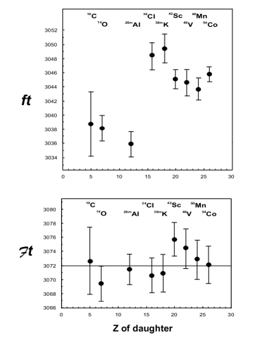
Figure 1: Comparison of experimental ft-values and the corrected ${\cal F}t$-values for the nine well-known superallowed transitions. This illustrates the effect of the calculated nucleus-dependent corrections, which change from transition to transition. (The effect of $\delta_{R}^{\prime}$ is virtually the same for all cases.)

We have argued that decreasing the radiative correction $\delta_{R}^{\prime}$ from 1.4% to 1.1%, or $\Delta_{\mbox{\tiny R}}^{\mbox{\tiny V}}$ from 2.4% to 2.1% is unlikely to be the solution to the CKM unitarity problem; and that there is no support from calculations for an average increase in the nuclear-structure dependent correction, ($\delta_{C}-\delta_{NS}$), from 0.5% to 0.8%. We are therefore confident that the unitarity result in Eq.(2), which is unchanged by our new calculations, incorporates structure-dependent corrections that are correct within their stated uncertainties. Nevertheless, these uncertainties are conservatively assigned and, as we remarked in the introduction, they contribute significantly to the overall uncertainty of the unitarity test. There is every reason to continue to focus on these corrections, both experimentally and theoretically, with a view to reducing their uncertainties still farther.

One way to do so, of course, would be to increase the precision of the $ft$-values for the nine cases tabulated in Table 8 and thus improve the comparison with CVC that is illustrated in Fig. 1. However, given the large amount of high-quality data that is already incorporated in these nine $ft$-values, significant improvements are unlikely in the near term. A more promising experimental approach to testing $\delta_{C}$ is offered by the possibility of increasing the number of superallowed emitters accessible to precision studies. Two series of $0^{+}$ nuclei present themselves: the even-$Z$, $T_{z}=-1$ nuclei with $18\leq A\leq 42$, and the odd-$Z$, $T_{z}=0$ nuclei with $A\geq 62$. The main attraction of these new regions is that the calculated values of $\delta_{C}-\delta_{NS}$ for the superallowed transitions are larger, or show larger variations from nuclide to nuclide, than the values applied to the nine currently well-known transitions (see Table 6). In principle, then, they afford a valuable test of the accuracy of the $\delta_{C}$ calculations. It is argued that if the calculations reproduce the experimentally observed variations where they are large, then that must surely verify their reliability for the original nine transitions whose $\delta_{C}$ values are considerably smaller. The calculations reported here, the only complete set available for all these new cases, should provide a sound basis to which new experimental data can be compared.

Currently, the greatest attention is being paid to the $T_{z}=0$ emitters with $A\geq 62$, since these nuclei are being produced at new radioactive-beam facilities, and their calculated $\delta_{C}$ corrections had previously been predicted to be large OB95 ; SVS96 . It is likely, though, that the required experimental precision will take some time to achieve. The decays of these nuclei are of higher energy and each therefore involves numerous weak Gamow-Teller transitions in addition to the superallowed transitionHT02 . Branching-ratio measurements will thus be very demanding, particularly with the limited intensities likely to be available initially for most of these rather exotic nuclei. In addition, their half-lives are considerably shorter than those of the lighter superallowed emitters; high-precision mass measurements ($\pm 2$ keV) for such short-lived activities will also be very challenging.

More accessible in the short term will be the $T_{z}=-1$ superallowed emitters with $18\leq A\leq 42$. There is good reason to explore them. For example, the calculated value of ($\delta_{C}-\delta_{NS}$) for ³⁰S decay, though smaller than those expected for the heavier nuclei, is actually 1.13% – larger than for any other case currently known – while ²²Mg has a low value of 0.51%. If such large differences are confirmed by the measured $ft$-values, then it will do much to increase our confidence in the calculated Coulomb corrections. To be sure, these decays will also provide a challenge, particularly in the measurement of their branching ratios, but the required precision should be achievable with isotope-separated beams that are currently available.

IV Conclusions

We have presented a new and consistent set of calculations for the nuclear-structure dependent corrections, ($\delta_{C}$ - $\delta_{NS}$), required in the analysis of superallowed $0^{+}\rightarrow 0^{+}$ beta decay. Twenty transitions have been included in our calculations, the nine well known ones already used in the CKM unitarity test, and eleven more that are likely to be accessible to precise measurements in the future. The unitarity test itself is unchanged by our calculations, one of several indications we offer that these corrections are under control within their stated uncertainties. We have also argued that the structure-independent radiative corrections are similarly sound. If the apparent deviation from unitarity is to be resolved without demanding some extension to the Standard Model, the only remaining possibility is through undiscovered errors in $V_{us}$, whose value is currently derived from $K_{e3}$ decayPDG00 ; LR84 and has not been revisited in nearly 20 years.

We have also shown that the uncertainty quoted for the unitarity test can most effectively be improved by reductions in the uncertainties of $\Delta_{\mbox{\tiny R}}^{\mbox{\tiny V}}$ and ($\delta_{C}-\delta_{NS}$). We have outlined an experimental method by which the latter can be improved, and have provided the full set of calculated corrections that can be tested against experiment. The stage is now set for a new influx of experimental results on previously unexplored superallowed transitions, from which the calculated structure-dependent corrections can be tested and confirmed or refined. In either case, the uncertainties should be reduced and the unitarity test sharpened.

Appendix A Effective Interactions

In the tables of results presented in the main text, we have only provided one set of values for each decay studied. However, for each nucleus, many calculations were performed with varying choices of effective interactions and shell-model spaces. The error assigned to the adopted values reflects the spread in the results and our estimate of the uncertainty in the calculated value based on the quality of the shell-model calculation.

The choice of an effective interaction is easily made for shell-model calculations in light nuclei whose principal configurations involve several valence nucleons away from major shell closures. There are well established interactions that give excellent fits to spectra. For $A=10$, we use the Cohen-KurathCK65 interaction, (8-16)POT, and for $A=22$, 26, 30 and 34, we use the universal $s,d$-interaction, USD, of WildenthalWi84 . For nuclei with $A=46$, 50 and 54, we considered two interactions: the Kuo-Brown $G$-matrixKB66 as modified by Poves and ZukerPZ81 and denoted KB3, and the $fp$-model independent interaction of Richter et al.Ri91 and denoted FPMI3. For nuclei with $A=50$ and 54 it was not possible to perform untruncated calculations in the full $fp$ space; our calculations only contain $(f_{7/2})^{n-r}(p_{3/2},f_{5/2},p_{1/2})^{r}$ configurations with $r\leq 2$. In this truncated calculation, the spectrum obtained for $0^{+}$ states in $A=50$ and 54 is in very poor agreement with experiment, a much larger energy gap between the ground state and first excited $0^{+}$ being obtained. Thus, we have made further adjustments to the interaction centroids to obtain a much improved spectrum in the truncated space.

For nuclei with $A=62$, 66 and 70 we considered the model space $(p_{3/2},f_{5/2},p_{1/2})^{n}$, with $n=A-56$, which is based on a closed $f_{7/2}$ shell at the ⁵⁶Ni core. This model space is the one used by Koops and Glaudemans KG77 in their study of nickel and copper isotopes. We found this model space, with a modified surface delta interaction (MSDI) as used in KG77 , gave acceptable spectra for the beta-decaying nuclei, with excited $0^{+}$ states at about the right excitation energy.

The problem cases were $A=14$, 18, 38, 42 and 74. In each of these cases, the experimental excited $0^{+}$ states are at a much lower energy than can be obtained in shell-model calculations. This is symptomatic of the presence of deformed configurations intruding among the spherical shell-model configurations. For example, in the $A=42$ spectrum the lowest-energy states are predominantly two particles outside a closed ⁴⁰Ca core, $|2p\rangle$, but lying low in the spectrum are ‘intruder’ states with a configuration of four particles and two holes, $|4p{\mbox{-}}2h\rangle$. Mixing between these configurations must occur, and it is difficult to obtain the correct degree of mixing with the shell model. Shell-model calculations that attempt to mix $|2p\rangle$ and $|4p{\mbox{-}}2h\rangle$ configurations encounter what has been called WB92 the “$n\hbar\omega$ catastrophe”. The presence of $|4p{\mbox{-}}2h\rangle$ configurations depresses the $|2p\rangle$ states, opening up a large energy gap between the $|2p\rangle$ and $|4p{\mbox{-}}2h\rangle$ states. This would be corrected somewhat if the model calculation included $|6p{\mbox{-}}4h\rangle$ states as well, since the role of the $|6p{\mbox{-}}4h\rangle$ states is to depress the $|4p{\mbox{-}}2h\rangle$ states. Thus if the model space is truncated to include only $|2p\rangle$ and $|4p{\mbox{-}}2h\rangle$ states, the depression driven by the $|6p{\mbox{-}}4h\rangle$ states on the $|4p{\mbox{-}}2h\rangle$ states is absent. In an attempt to circumvent this catastrophe we weakened the cross-shell interactions. Specifically, at mass 14, 18, 38 and 42 we used the Millener-Kurath MK75 interaction to evaluate the $\langle 2p|V|4p{\mbox{-}}2h\rangle$ matrix elements. We multiplied these matrix elements by a factor, $f$, that ranges from 0.0 to 1.0. When $f=0.0$, there is no mixing between $|2p\rangle$ and $|4p{\mbox{-}}2h\rangle$ configurations, and when $f=0.6$ the ground-state wave function is approximately $80\%|2p\rangle$ and $20\%|4p{\mbox{-}}2h\rangle$. Our strategy was to adjust $f$ so that the excited $0^{+}$ energy is approximately equal to the experimental excitation energy. We have examined the sensitivity of our results to variations in $f$ and ensured that the spread of values obtained were within the assigned errors attributed.

There are some older interactions that operate in very restrictive model spaces, but remove the $n\hbar\omega$ catastrophe by allowing mixing between $|2p\rangle$, $|4p{\mbox{-}}2h\rangle$ and $|6p{\mbox{-}}4h\rangle$ configurations. These are the Zuker-Buck-McGroryZBM68 interaction, ZBM, as modified by Zuker Zu69 , which uses the $p_{1/2}$, $s_{1/2}$ and $d_{5/2}$ orbitals for the $A=14$ and 18 nuclei; and the Federman-PittelFP69 interaction, FP, which uses the $d_{3/2}$ and $f_{7/2}$ orbitals for the $A=38$ and 42 nuclei.

Finally, at mass 74 there is a related but slightly different problem. The spectrum in a $(p_{3/2},f_{5/2},p_{1/2})^{18}$ model space gives about the right density of natural-parity states. The difficulty is the presence of unnatural-parity states lying low in the spectrum (for example, ⁷³Br has a $5/2^{+}$ at only 280 keV excitation, while ⁷⁵Rb has a probable $3/2^{+}$ at 40 keV). Further, the excited $0^{+}$ state in ⁷⁴Kr is at only 508 keV, whereas the $(p_{3/2},f_{5/2},p_{1/2})^{18}$ model calculation puts the state at 2550 keV. The influence of the $1g_{9/2}$, $2d_{5/2}$ and possibly $1g_{7/2}$ orbitals is evidently quite strong at the end of the $p,f$ shell. Thus, we have used the following model space

$$(p_{3/2},f_{5/2},p_{1/2})^{18}+(p_{3/2})^{8}(f_{5/2},p_{1/2})^{8}(g_{9/2},d_{5/2},g_{7/2})^{2}.$$ (26)

Let us call the first term in Eq. (26) the $0\hbar\omega$ term, and the second term with two nucleons promoted to the $d,g$ shell the $2\hbar\omega$ term. Because of the “$n\hbar\omega$ catastrophe”, we again multiply all $\langle 0\hbar\omega|V|2\hbar\omega\rangle$ matrix elements by a factor, $f$, and adjust $f$ so that the excited $0^{+}$ state in ⁷⁴Kr is reproduced at its experimental location. All matrix elements were then calculated with the MSDI interactionKG77 .

References

- (1) I.S. Towner and J.C. Hardy, Proc. of the V Int. WEIN Symposium: Physics Beyond the Standard Model, Santa Fe, NM, June 1998, edited by P. Herczeg, C.M. Hoffman and H.V. Klapdor-Kleingrothaus (World Scientific, Singapore, 1999) pp. 338-359.
- (2) J.C. Hardy, I.S. Towner, V.T. Koslowsky, E. Hagberg and H. Schmeing, Nucl. Phys. A509, 429 (1990).
- (3) H. Abele, M.A. Hoffmann, S. Baessler, D. Dubbers, F. Gluck, U. Muller, V. Nesvizhevsky, J. Reich and O. Zimmer, Phys. Rev. Lett. 88, 211801 (2002).
- (4) D.E. Groom et al., Eur. Phys. J. C 15, 1 (2000).
- (5) A. Sirlin, Phys. Rev. D35, 3423 (1987); A. Sirlin and R. Zucchini, Phys. Rev. Lett. 57, 1994 (1986).
- (6) W. Jaus and G. Rasche, Phys. Rev. D35, 3420 (1987).
- (7) W.E. Ormand and B.A. Brown, Nucl. Phys. A440, 274 (1985).
- (8) E. Hagberg, V.T. Koslowsky, J.C. Hardy, I.S. Towner, J.G. Hykawy, G. Savard and T. Shinozuka, Phys. Rev. Lett. 73, 396 (1994).
- (9) I.S. Towner, J.C. Hardy and M. Harvey, Nucl. Phys. A284, 269 (1977).
- (10) A. Sirlin, Phys. Rev. 164, 1767 (1967).
- (11) W.J. Marciano and A. Sirlin, Phys. Rev. Lett. 56, 22 (1986).
- (12) A. Sirlin, in Precision Tests of the Standard Electroweak Model, ed. P. Langacker (World-Scientific, Singapore, 1994).
- (13) W. Jaus and G. Rasche, Phys. Rev. D41, 166 (1990).
- (14) F.C. Barker, B.A. Brown, W. Jaus and G. Rasche, Nucl. Phys. A540, 501 (1992).
- (15) I.S. Towner, Nucl. Phys. A540, 478 (1992).
- (16) I.S. Towner, Phys. Lett. B333, 13 (1994).
- (17) I.S. Towner, Phys. Reports 155, 263 (1987).
- (18) A. Arima, K. Shimizu, W. Bentz and H. Hyuga, Adv. in Nucl. Phys. 18, 1 (1987).
- (19) B.A. Brown and B.H. Wildenthal, Phys. Rev. C28, 2397 (1986); B.A. Brown and B.H. Wildenthal, At. Data Nucl. Data Tables 33, 347 (1985); B.A. Brown and B.H. Wildenthal, Nucl. Phys. A474, 290 (1987).
- (20) P. Navrátil, B.R. Barrett and W.E. Ormand, Phys. Rev. C56, 2542 (1997).
- (21) J. Britz, A. Pape and M.S. Antony, Atomic Data and Nucl. Data Tables 69, 125 (1998).
- (22) W.E. Ormand and B.A. Brown, Phys. Rev. Lett. 62, 866 (1989).
- (23) W.W. Daehnick and R.D. Rosa, Phys. Rev. C31, 1499 (1985).
- (24) H. De Vries, C.W. De Jager and C. De Vries, Atomic Data and Nucl. Data Tables 36, 495 (1987).
- (25) I.S. Towner and J.C. Hardy, Nucl. Phys. A205, 33 (1973).
- (26) I.S. Towner, in Symmetry Violations in Subatomic Physics, edited by B. Castel and P.J. O’Donnel (World Scientific, Singapore, 1989), p. 211.
- (27) W.E. Ormand and B.A. Brown, Phys. Rev. C52, 2455 (1995).
- (28) H. Sagawa, N. Van Giai and T. Suzuki, Phys. Rev. C53, 2163 (1996).
- (29) J.C. Hardy and I.S. Towner Phys. Rev. Lett. 88, 252501 (2002).
- (30) H. Leutwyler and M. Roos, Z. Phys. C25, 91 (1984).
- (31) S. Cohen and D. Kurath, Nucl. Phys. 73, 1 (1965).
- (32) B.H. Wildenthal, in Progress in Particle and Nuclear Physics, edited by D.H. Wilkinson (Pergamon Press, Oxford 1984) Vol. 11, p. 5.
- (33) T.T.S. Kuo and G.E. Brown, Nucl. Phys. 85, 40 (1966).
- (34) A. Poves and A.P. Zuker, Phys. Reports 70, 235 (1981).
- (35) W.A. Richter, M.G. Van Der Merwe, R.E. Julies and B.A. Brown, Nucl. Phys. A523, 325 (1991).
- (36) J.E. Koops and P.W.M. Glaudemans, Z. Phys. A280, 181 (1977).
- (37) E.K. Warburton and B.A. Brown, Phys. Rev. C46, 923 (1992).
- (38) D.J. Millener and D. Kurath, Nucl. Phys. A255, 315 (1975).
- (39) A.P. Zuker, B. Buck and J.B. McGrory, Phys. Rev. Lett. 21, 39 (1968).
- (40) A.P. Zuker, Phys. Rev. Lett. 23, 983 (1969).
- (41) P. Federman and S. Pittel, Phys. Rev. 186, 1106 (1969).