Abstract

We evaluate the two pion decay of the Roper resonance in a model where explicit re-scattering of the two final pions is accounted for by the use of unitarized chiral perturbation theory. Our model does not include an explicit $\epsilon$ or $\sigma$ scalar-isoscalar meson decay mode, instead it generates it dynamically by means of the pion re-scattering. The two ways, explicit or dynamically generated, of introducing this decay channel have very different amplitudes. Nevertheless, through interference with the other terms of the model we are able to reproduce the same phenomenology as models with explicit consideration of the $\epsilon$ meson.

1 Introduction

The Roper resonance is one of the controversial resonances, with an abnormally large width comparative to other resonances with larger mass. It appears naturally in quark models with a radial excitation of one of the quarks [1, 2, 3], but it has also been suggested that it is dynamically generated by the meson-baryon interaction itself [4] and thus would be essentially formed by a large meson-nucleon cloud. One of the intriguing properties of the Roper is its two pion decay mode. According to the PDG [5], it has a 30-40 percent branching ratio into $N\pi\pi$, mostly going to $\Delta\pi$, and a small fraction of 5-10 percent which goes into a nucleon and two pions in s-wave and isospin, I=0. This scalar isoscalar mode plays a very important role in all reactions involving two pion production close to threshold. The reason is that the contribution from the nucleon intermediate states cancels at threshold when the direct and crossed terms are taken into account. Then the next resonance which is the $\Delta$ involves p-wave couplings which would vanish at threshold, and finally comes the Roper, which thanks to this non vanishing scalar isoscalar decay mode into two pions gives a non vanishing contribution to the threshold amplitudes. This has been shown explicitly to be the case in pion induced two pion production [6, 7, 8, 9], photon induced two pion production [10, 11] and two pion production in nucleon nucleon collisions [12, 13, 14, 15]. The influence of the Roper excitation and its decay modes in many other reactions has been discussed in [16, 17, 18]. Similarly, it has also been shown [19, 20] in the study of the Roper excitation in the ($\alpha,\alpha^{\prime}$) reaction that the Roper is very efficiently excited by an isoscalar source, which should somehow be related to this scalar isoscalar decay.

The evidence for this scalar isoscalar two pion decay comes mostly from the analysis of Manley [21, 22], where he fits the data by means of the excitation of an $\epsilon$ meson of about 800 MeV mass and width plus the decay into $\Delta\pi$. This $\epsilon$ meson is what we would call now the $\sigma$ meson, or in an alternative nomenclature, the $f_{0}(400-900)$ meson, as also used in the PDG. However, the immediate conceptual problem arises, since, whatever this meson is called, the strength of the two pion distribution does not follow the shape provided by the exchange of such a heavy and broad meson. The isoscalar two pion distribution at low energies is governed by the scattering matrix of two pions in L=0, I=0, which has a broad bump consisting of a large background on top of the effects of the $\sigma$ pole, which is now present in all modern theoretical [23, 24, 25] and experimental analyses [26, 27], (see also the proceedings of the $\sigma$ Workshop [28] ). The pole of the $\sigma$ appears in all these approaches with a mass around 500 MeV and a width around 400 MeV, and, as mentioned above, there is also a large background present in the $\pi\pi$ t-matrix.

In the present context it is also worth mentioning that the use of chiral perturbation theory [29] and its unitary extensions in coupled channels [23, 24, 30, 31, 32, 33, 34] has brought a new perspective on the nature of the scalar meson resonances, in particular the $\sigma$. Indeed, what is found in these works is that the $\sigma$ is generated dynamically from the lowest order chiral Lagrangian and the multiple scattering of the mesons implicit in the unitary approach. This finding and the previous statement is more than semantics, because it implies that anything having to do with the production of a $\sigma$ should be considered as the production of two pions which undergo final state interaction (in this case in the strong L=0, I=0 channel). This is the philosophy taken in the present work, where we perform a theoretical study of the two pion decay of the Roper, with the explicit consideration of the final state interaction of the two pions, which automatically generates the production of this two pion $\sigma$ mode. The approach is hence different to the one followed in [21, 22] since we do not allow the direct production of a $\sigma$. Yet, we aim at reproducing the same phenomenology that was fitted in the analysis of [21, 22]. We will show how this is possible, and even if a very different, and obviously more realistic, distribution of the two pion invariant mass is obtained for the scalar isoscalar decay mode, the coherent sum of the different mechanisms that we have leads to mass distributions of the two pions or of one pion-nucleon system, in agreement with the results that one would obtain with Manley’s approach of $\Delta\pi$ plus the massive and broad $\epsilon$ meson production.

2 Manley’s approach for the two pion decay of the Roper

In this section we will translate the two pion decay model of the Roper described in refs. [21, 22] to the language of Lagrangian and Feynman diagrams. As explained in the introduction, the model has two intermediate decay channels for the Roper decay into two pions: the Roper can decay either into an intermediate $\Delta\pi$ state or into an intermediate $N\epsilon$ state. The $\epsilon$ meson is a scalar isoscalar meson with a mass and width of $M_{\epsilon}\!=\!\Gamma_{\epsilon}(M_{\epsilon})\!=\!800$ MeV. The Feynman diagrams for the two decaying modes appear in Fig. 1a-b.

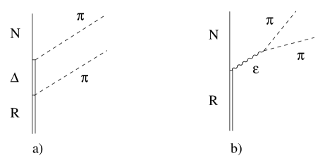
Figure 1: Feynman diagrams for the two processes contributing to the Roper decay into two pions in Manley’s approach. a) $\Delta\pi$ intermediate channel. b) $N\epsilon$ intermediate channel.

In the spirit of refs. [21, 22] we will use here non relativistic Lagrangian for the different vertices involved in the calculation. Those Lagrangian are given, with obvious notation, as

$${\cal L}_{R\Delta\pi}(x) = \frac{f_{R\Delta\pi}}{m_{\pi}}\Psi^{\dagger}_{\Delta}(x)S^{\dagger}_{j}{\bf T}^{\dagger}(\partial_{j}\hbox{$\pi$}\hbox to0.0pt{\hss\hbox{$\pi$}\hskip 0.39993pt}\hbox to0.0pt{\hss\lower 0.17218pt\hbox{\hbox{$\pi$}\hbox to0.0pt{\hss\hbox{$\pi$}\hskip 0.39993pt}}}(x))\Psi_{R}(x)\,\epsilon(x)$$

$${\cal L}_{\Delta N\pi}(x) = \frac{f_{\Delta N\pi}}{m_{\pi}}\Psi^{\dagger}_{N}(x)S_{j}{\bf T}(\partial_{j}\hbox{$\pi$}\hbox to0.0pt{\hss\hbox{$\pi$}\hskip 0.39993pt}\hbox to0.0pt{\hss\lower 0.17218pt\hbox{\hbox{$\pi$}\hbox to0.0pt{\hss\hbox{$\pi$}\hskip 0.39993pt}}}(x))\Psi_{\Delta}(x)$$ (1)

and

$${\cal L}_{RN\epsilon}(x) = g_{RN\epsilon}\Psi^{\dagger}_{N}(x)\Psi_{R}(x)\,\epsilon(x)$$

$${\cal L}_{\epsilon\pi\pi}(x) = g_{\epsilon\pi\pi}\ \epsilon(x)\,\hbox{$\pi$}\hbox to0.0pt{\hss\hbox{$\pi$}\hskip 0.39993pt}\hbox to0.0pt{\hss\lower 0.17218pt\hbox{\hbox{$\pi$}\hbox to0.0pt{\hss\hbox{$\pi$}\hskip 0.39993pt}}}(x)\,\hbox{$\pi$}\hbox to0.0pt{\hss\hbox{$\pi$}\hskip 0.39993pt}\hbox to0.0pt{\hss\lower 0.17218pt\hbox{\hbox{$\pi$}\hbox to0.0pt{\hss\hbox{$\pi$}\hskip 0.39993pt}}}(x)$$ (2)

${\bf S}^{\dagger}$ and ${\bf T}^{\dagger}$ are respectively the spin and isospin operators for the 1/2 to 3/2 transition with matrix elements just given by Clebsch-Gordan coefficients.

The amplitude for the process in Fig. 1a is given by

$${\cal M}_{1a} = i\,\frac{f_{R\Delta\pi}}{m_{\pi}}\,\frac{f_{\Delta N\pi}}{m_{\pi}}\ \Phi_{N}^{\dagger}\chi_{N}^{\dagger}$$ (3)

$$\bigg{[}\ \hskip 11.38092pt\bigg{(}\frac{2}{3}\,{\bf q}_{1}\cdot{\bf q}_{2}-\frac{i}{3}\,\hbox{$\sigma$}\hbox to0.0pt{\hss\hbox{$\sigma$}\hskip 0.39993pt}\hbox to0.0pt{\hss\lower 0.17218pt\hbox{\hbox{$\sigma$}\hbox to0.0pt{\hss\hbox{$\sigma$}\hskip 0.39993pt}}}\cdot({\bf q}_{1}\times{\bf q}_{2})\bigg{)}\ \bigg{(}\frac{2}{3}\,\delta_{j_{1}j_{2}}-\frac{i}{3}\,\varepsilon_{j_{1}j_{2}k}\cdot\tau_{k}\bigg{)}$$

$$\hskip 11.38092pt\frac{M_{\Delta}}{E_{\Delta}({\bf q}_{1})}\ \frac{1}{M_{R}-q_{1}^{0}-E_{\Delta}({\bf q}_{1})+\frac{i}{2}\,\Gamma_{\Delta}(p_{R}-q_{1})}$$

$$+(1\leftrightarrow 2)\hskip 11.38092pt\bigg{]}\,\Phi_{R}\chi_{R}$$

$\Phi$ and $\chi$ are respectively isospin and spin Pauli spinors for both the nucleon and the Roper while $\tau$$\tau$ $\tau$$\tau$  and $\sigma$$\sigma$ $\sigma$$\sigma$  are the isospin and spin Pauli matrices. $p_{R}=(M_{R},{\bf 0})$, $q_{1}$ and $q_{2}$ are the four-momentum of the Roper and the two pions, and $E_{\Delta}({\bf q})$ is the on-shell energy of a $\Delta$ with three-momentum ${\bf q}$. Finally $j_{1}$ and $j_{2}$ are isospin indices in the cartesian base for the two pions. Note that since we are working in the isospin mathematical base the pions are identical particles and the amplitude has to be symmetrized with respect to the exchange of the pions. In the expression for the width we have to include a factor $1/2$ of symmetry. For the process in Fig. 1b we get

$${\cal M}_{1b}=-2i\,g_{RN\epsilon}\,g_{\epsilon\pi\pi}\ \frac{1}{s-M_{\epsilon}^{2}+i\,M_{\epsilon}\,\Gamma_{\epsilon}(s)}\ \Phi_{N}^{\dagger}\cdot\Phi_{R}\ \ \chi_{N}^{\dagger}\cdot\chi_{R}\hskip 8.5359pt\delta_{j_{1}j_{2}}$$ (4)

where $s$ is the total four-momentum square of the two final pions. Even though the previous amplitudes are non-relativistic for the phase space integrals we shall take into account all the appropriate relativistic factors. As for the coupling constants we fix $f_{\Delta N\pi}$ from the width of the $\Delta$ as given by the PDG. A value of $f_{\Delta N\pi}\!=\!2.07$ results. For the other coupling constants one needs information on the width of the Roper associated to the two channels involved. Those values and the mass of the Roper we take from Manley’s analysis. Comparing $\Gamma_{R\to\Delta\pi}\!=\!88$ MeV to the result obtained with the use of the Feynman diagram of Fig. 1a one gets $f_{R\Delta\pi}\!=\!1.56$, while from $\Gamma_{R\to N\epsilon}\!=\!33$ MeV and the evaluation of the contribution due to the Feynman diagram in Fig. 1b one determines the product of coupling constants $g_{RN\epsilon}\cdot g_{\epsilon\pi\pi}\!=\!1.43\cdot 10^{-2}$ $M_{\epsilon}^{2}$ MeV^-1. The sign of this product of coupling constants relative to $f_{R\Delta\pi}$ is chosen to be positive in accordance with the sign assignment done in [22]. Note also that for the first process the pions can be in both $I=0,1$ isospin states while for the second only $I=0$ is allowed. The total width for the Roper decay into two pions that we get when taking into account both terms is given by $\Gamma_{R\to N\pi\pi}\!=\!153$ MeV, meaning that there is constructive interference between the two contributions. While this interference effect is also present in the amplitude used in ref. [22] there the total width is taken to be $\Gamma_{R\to N\pi\pi}\!=\Gamma_{R\to\Delta\pi}+\Gamma_{R\to N\epsilon}=121$ MeV.

Figure 2: $\pi-\pi$ invariant mass distributions as obtained in Manley’s approach. Dashed line: distribution obtained from considering the $\Delta\pi$ intermediate channel alone. Dotted line: distribution obtained from considering the $N\epsilon$ intermediate channel alone. Full curve: total result.

In Fig. 2 we give two-pion invariant mass distributions obtained within the approach just described. The distribution that arises from considering the intermediate channel $N\epsilon$ alone is represented by the dotted line and it is essentially given by phase space. The dashed line gives now the distribution corresponding to the intermediate $\Delta\pi$ state. There one sees two peaks at large and small invariant masses that are due to the presence of a $(\vec{q}_{1}\cdot\vec{q}_{2})^{2}$ term, with $\vec{q}_{1,2}$ the three-momentum of the pions, in the amplitude square (see Eq. (3)). The maximum for this quantity is reached when the two pions move in the same direction (small invariant mass) or in opposite direction (large invariant mass). The invariant mass distribution corresponding to the coherent sum of the two channels is given by the full curve. The interference effect is clearly seen at large and small invariant masses. While the peak at large invariant mass increases the one at low invariant mass decreases.

In Fig. 3 we show pion-nucleon invariant mass distributions. As before the $N\epsilon$ contribution is basically given by phase space, while the $\Delta\pi$ one shows a peak below the Delta mass. In the total contribution the central peak is enhanced due to interference.

Figure 3: $\pi-N$ invariant mass distributions as obtained in Manley’s approach. Notation as in Fig. 2.

As these invariant mass distributions are obtained from amplitudes that are fitted to experiment we will consider them as if they were true “experimental results” to which we can compare our own results.

3 Model for the two pion decay of the Roper

In our model we will consider two types of contributions. In the first type, that we shall call open-diagrams contribution, the Roper decays into a baryon and a pion and then the baryon decays into nucleon-pion. No final state interaction between the two pions is considered. For the intermediate baryon we take Delta, nucleon and Roper itself.

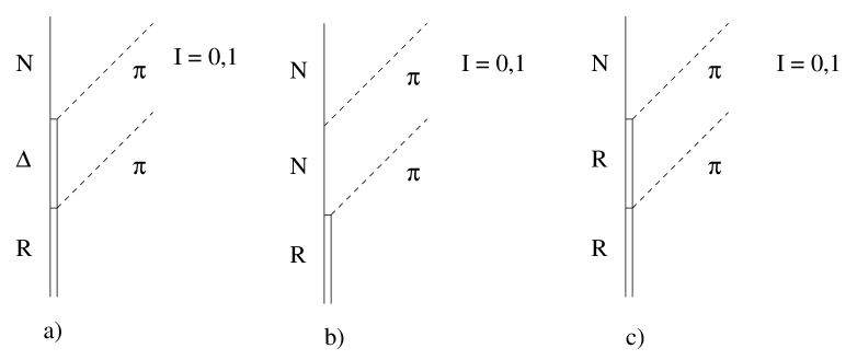
Figure 4: Feynman diagrams corresponding to our “open-diagrams” contribution to the Roper decay into two pions. Diagrams a), b) and c) correspond to taking Delta, nucleon or Roper as intermediate baryons. The two final pions can be in both $I=0,1$ isospin states.

This contribution, whose Feynman diagrams appear in Fig. 4, is the equivalent in our model of the $\Delta\pi$ intermediate channel in Manley’s approach. The differences come from the fact that we include also $N\pi$ and $R\pi$ intermediate states and we take into account relativistic corrections for the vertices involved. Those relativistic corrections are given for the $N^{\prime}\to N\pi$ transition as

$$\hbox{$\sigma$}\hbox to0.0pt{\hss\hbox{$\sigma$}\hskip 0.39993pt}\hbox to0.0pt{\hss\lower 0.17218pt\hbox{\hbox{$\sigma$}\hbox to0.0pt{\hss\hbox{$\sigma$}\hskip 0.39993pt}}}\cdot{\bf q}\to\hbox{$\sigma$}\hbox to0.0pt{\hss\hbox{$\sigma$}\hskip 0.39993pt}\hbox to0.0pt{\hss\lower 0.17218pt\hbox{\hbox{$\sigma$}\hbox to0.0pt{\hss\hbox{$\sigma$}\hskip 0.39993pt}}}\cdot{\bf q}\ (1-\frac{q^{0}}{2M^{\prime}})-\hbox{$\sigma$}\hbox to0.0pt{\hss\hbox{$\sigma$}\hskip 0.39993pt}\hbox to0.0pt{\hss\lower 0.17218pt\hbox{\hbox{$\sigma$}\hbox to0.0pt{\hss\hbox{$\sigma$}\hskip 0.39993pt}}}\cdot{\bf p}\ (\frac{q^{0}}{2M^{\prime}}+\frac{q^{0}}{2M})$$ (5)

where $N^{\prime},N$ stand for either nucleon or Roper, $(q^{0},{\bf q})$ is the pion four momentum and ${\bf p}$ the three-momentun of the final $N$. This comes automatically from the evaluation of the matrix elements of the $\gamma^{\mu}\gamma_{5}\partial_{\mu}$ operator of the pseudovector coupling of the pions to the nucleons. For the vertices involving $\Delta$ we take the Lagrangian of Eq. 2, where it has been implicitly assumed the $\Delta$ to be at rest, and introduce the appropriate modification

$${\bf S}^{\dagger}\cdot{\bf q}\to{\bf S}^{\dagger}\cdot({\bf q}-\frac{q^{0}}{M_{\Delta}}\,{\bf p}_{\Delta})$$

$${\bf S}\cdot{\bf q}\to{\bf S}\cdot({\bf q}-\frac{q^{0}}{M_{\Delta}}\,{\bf p}_{\Delta})$$ (6)

For the coupling constants we take $f_{NN\pi}=g_{A}\frac{m_{\pi}}{2f_{\pi}}=0.95$, the naive quark model result $f_{RR\pi}=f_{NN\pi}$, and for $f_{RN\pi}$ we use the experimental information on $\Gamma_{R\to N\pi}=270$ MeV from which $f_{RN\pi}=0.40$. We still have to fix $f_{R\Delta\pi}$.

For that we need our second type of contribution, that we call closed-diagrams contribution, and that we construct by allowing the two pions in the final state to re-scatter in the $I=0$ isospin channel. The corresponding Feynman diagrams appear in Fig. 5 and this is our model analogue of the $N\epsilon$ channel in Manley’s analysis.

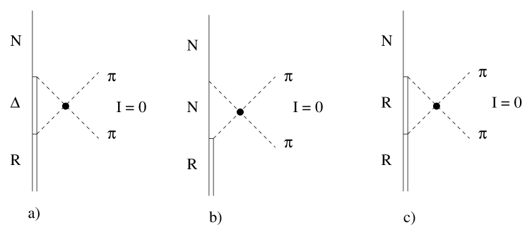
Figure 5: Feynman diagrams corresponding to our “closed-diagrams” contribution to the Roper decay into two pions. a), b) and c) as in Fig. 4. The big dot represents the $\pi\pi$ t-matrix in the $I=0$ channel. Re-scattering in the $I=1$ channel is neglected.

To fully define our model we have to give the form factors that we use to regularize the loop integrals and also the $\pi\pi$ t-matrix for the channel $L=0,I=0$. The latter will be given in the next subsection. For each of the baryon-baryon-pion vertices we take a monopole form factor

$$F({\bf q})=\frac{\Lambda^{2}}{\Lambda^{2}+{\bf q}^{2}}$$ (7)

with the same value of $\Lambda$ for all cases. We will discuss the cut-off dependence in the results section.

As an illustration we give the amplitude corresponding to the process in Fig. 5a

$${\cal M}_{5a} = \frac{2}{3\sqrt{3}}\ \frac{f_{R\Delta\pi}}{m_{\pi}}\,\frac{f_{\Delta N\pi}}{m_{\pi}}\ \Phi_{N}^{\dagger}\ \chi_{N}^{\dagger}\ \bigg{\{}\int\frac{d^{4}q}{(2\pi)^{4}}$$ (8)

$$\bigg{\{}\ \bigg{[}\ \ \bigg{(}\frac{2}{3}\,({\bf p}_{N}-{\bf q})\cdot{\bf q}-\frac{i}{3}\,\hbox{$\sigma$}\hbox to0.0pt{\hss\hbox{$\sigma$}\hskip 0.39993pt}\hbox to0.0pt{\hss\lower 0.17218pt\hbox{\hbox{$\sigma$}\hbox to0.0pt{\hss\hbox{$\sigma$}\hskip 0.39993pt}}}\cdot(({\bf p}_{N}-{\bf q})\times{\bf q})\bigg{)}\bigg{(}1+\frac{M_{R}}{M_{\Delta}}-\frac{q^{0}}{M_{\Delta}}\bigg{)}$$

$$+\ \frac{2}{3}\ {\bf q}^{2}\ \frac{q^{0}-p_{N}^{0}}{M_{\Delta}}\ \bigg{]}\ \frac{M_{\Delta}}{E_{\Delta}({\bf q})}\ \frac{1}{q^{0}-E_{\Delta}({\bf q})+\frac{i}{2}\,\Gamma_{\Delta}(q)}$$

$$\frac{1}{(p_{N}^{0}-q^{0})^{2}-({\bf p}_{N}-{\bf q})^{2}-m^{2}_{\pi}+i\varepsilon}\$$

$$\frac{1}{(M_{R}-q^{0})^{2}-{\bf q}^{2}-m^{2}_{\pi}+i\varepsilon}\ \frac{\Lambda^{2}}{\Lambda^{2}+({\bf p}_{N}-{\bf q})^{2}}\ \frac{\Lambda^{2}}{\Lambda^{2}+{\bf q}^{2}}\ \bigg{\}}$$

$$t^{I=0}_{\pi\pi}(s)\ \ \bigg{\}}\ \Phi_{R}\ \chi_{R}$$

Here $q$ and $p_{N}$ are respectively the four-momentum of the $\Delta$ in the loop and of the final nucleon. For the two final pions we have already taken into account the fact that they are in an $I=0$ isospin state. Similar results are obtained for the case of intermediate nucleon (Fig. 5b) or Roper (Fig. 5c). All baryon propagators that we use throughout the paper contain a momentum dependent imaginary part. In all cases we use the expression for the width corresponding to the $N\pi$ decay channel. For the Roper we re-scale that result to its total width.

We fix the $f_{R\Delta\pi}$ coupling constant by fitting with our full model, including the $\pi\pi$ t-matrix given in the next subsection, the total Roper decay width into two pions. For this width we take $\Gamma_{R\to N\pi\pi}=153$ MeV as evaluated in the previous section and obtain a coupling constant that depends on the cut-off $\Lambda$. The best agreement with the invariant mass distributions is obtained with $\Lambda=0.7$ GeV which gives $f_{R\Delta\pi}=1.1$ to be compared to 1.56 obtained in Manley’s approach. Larger $\Lambda$ values as those used in ref. [35] also agree reasonably with data.

3.1 $\pi\pi$ t-matrix in the $L=0,I=0$ channel

The $\pi\pi$ t-matrix in the $L=0,I=0$ channel we take from refs. [23, 24] where they use a non-perturbative approach that combines pion-pion potentials provided by the lowest order chiral Lagrangian with the Lipmann-Schwinger equation. The pion-pion potential corresponding to Fig. 6 is given by

$$V_{\pi\pi}^{I=0}=-\frac{6}{f_{\pi}^{2}}\bigg{(}s-\frac{m_{\pi}^{2}}{2}-\frac{1}{3}\sum_{j}(q_{j}^{2}-m_{\pi}^{2})\bigg{)}$$ (9)

where $f_{\pi}=92.4$ MeV is the pion decay constant and $\sqrt{s}$ gives the total energy in the center of mass. We give the potential separated into on-shell plus off-shell parts.

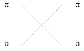
Figure 6: Feynman diagram for the $\pi\pi$ potential.

To obtain the t-matrix one sums an infinite set of diagrams where pions are allowed to re-scatter in the s-channel. Formally on can write this Lipmann-Schwinger equation as

$$t_{\pi\pi}^{I=0}=V_{\pi\pi}^{I=0}+V_{\pi\pi}^{I=0}\cdot G\cdot t_{\pi\pi}^{I=0}$$ (10)

where $G$ stands for the loop in Fig. 7.

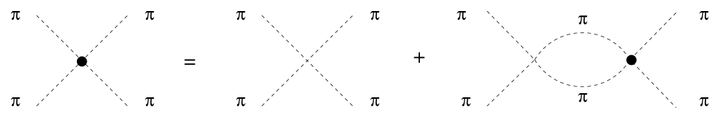
Figure 7: Set of Feynman diagrams corresponding to the Lipmann-Schwinger equation used to evaluate the $\pi\pi$ t-matrix in the $I=0$ channel. The contribution of kaons in the loop is neglected.

As shown in ref. [23] the use of the off-shell part of the potential amounts to a renormalization of $f_{\pi}$ and the pion mass and then it should not be included if one uses the physical values for those quantities. In that case Eq.(10) is purely algebraic and the factor $G$ is given by

$$G(s=P^{2})=\frac{i}{6}\int\frac{d^{4}q}{(2\pi)^{4}}\ \frac{1}{q^{2}-m_{\pi}^{2}+i\varepsilon}\ \frac{1}{(P-q)^{2}-m_{\pi}^{2}+i\varepsilon}$$ (11)

where $P$ is the total four-momentum of the two incoming (outgoing) pions. The integral is divergent and has to be regularized. Here we follow ref. [24] where dimensional regularization is used. The regularization mass, that is treated in ref. [24] as a free parameter, is given by $\mu=1.2$ GeV. The final expression for $G(s)$ is

$$G(s)=\frac{1}{6\,(4\pi)^{2}}\bigg{(}-1+\ln\frac{m_{\pi}^{2}}{\mu^{2}}+\sigma\ln\frac{\sigma+1}{\sigma-1}-i\pi\sigma\bigg{)}$$ (12)

where $\sigma=\sqrt{1-4m_{\pi}^{2}/s}$, and then

$$t_{\pi\pi}^{I=0}=-\frac{6}{f_{\pi}^{2}}\frac{s-m_{\pi}^{2}/2}{1+\frac{1}{f_{\pi}^{2}}(s-m_{\pi}^{2}/2)G(s)}$$ (13)

We shall use this on-shell t-matrix even though the two pions in the loop in Fig. 7 can be off-shell. It has been shown in ref. [35] that for the case of only nucleons and Deltas involved the dominant off-shell contribution is canceled exactly by considering, at the same order in the chiral counting, diagrams that contain vertices with one baryon line and three pions. By analogy a three pion vertex involving the Roper should also be included to produce this cancellation in the Roper case. Hence, as in [35], we shall only take the on shell part of the $\pi\pi$ interaction.

4 Results and discussion

In Table 1 we show the contribution to the Roper decay width into two pions of our open- and closed-diagrams mechanisms for $\Lambda=0.7$ GeV. Unless otherwise indicated all results correspond to this cut-off value. The results that we obtain are compared to the contributions of the equivalent $\Delta\pi$ and $N\epsilon$ mechanisms in Manley’s approach. The role of the mechanisms is different in the two models.

Our model		Manley’s approach
$\bullet$ Open-diagrams	55.3	$\bullet$  $\Delta\pi$	88
- Delta alone	54.7
- No Delta	0.6
$\bullet$ Closed-diagrams	68.6	$\bullet$  $N\epsilon$	33
- Delta alone	31.8
- No Delta	8.2
$\bullet$ Coherent sum	153	$\bullet$  Coherent sum	153

Table 1: Contribution of the different mechanisms to the two-pion Roper decay width. All numbers are in MeV. “Delta alone” in our model results means that we consider the Delta as the only intermediate baryon. “No Delta” in our model results means that we take only nucleon and Roper as intermediate baryons. Note the constructive interference between the “Delta alone” and “No Delta” contributions in the Closed-diagrams case.

While in Manley’s approach the dominant contribution comes from the $\Delta\pi$ mechanism in our case the closed-diagrams contribution, whose analogue in Manley’s analysis is the $N\epsilon$ channel, is larger. Also from the numbers in Table 1 one sees that in our model the largest contribution to the width comes from considering the Delta to be the intermediate baryon. The contribution that comes from considering intermediate nucleon and Roper is very small and only for the case of closed-diagrams the interference with the dominant intermediate Delta contribution is of some relevance.

Figure 8: $\pi-\pi$ invariant mass distributions as obtained in our model. Dashed line: distribution obtained from considering the open-diagrams contribution alone. Dotted line: distribution obtained from considering the closed-diagrams contribution alone. Full curve: total result.

In Fig. 8 we show now the two-pion invariant mass distribution obtained in our model. The dashed line corresponds to the open-diagrams contribution. One sees the two peak structure associated to the presence of the Delta. Compared to the $\Delta\pi$ distribution in Manley’s approach we see that the peak at high invariant mass is reduced in our case. This is due to the relativistic corrections present in our model. The dotted line corresponds to the closed-diagrams contribution. It has a broad peak at high invariant mass while it goes to zero at low invariant mass. Its shape is totally different from the phase space shape of the corresponding $N\epsilon$ contribution in Manley’s analysis. These differences notwithstanding, we see that the distribution that corresponds to the coherent sum of the two channels resembles very much what one gets in Manley’s approach. The two total distributions are compared now in Fig. 9 where one sees a good agreement between the two different approaches. Also in Fig. 9 we show the results for other values of the cut-off. This gives an idea of the theoretical uncertainties in our calculation.

Figure 9: Comparison of the $\pi-\pi$ invariant mass distributions as obtained in the two models. Dashed line: Manley’s approach distribution. Our model result: with $\Lambda=0.7$ GeV $(f_{R\Delta\pi}=1.1$) solid line, $\Lambda=0.9$ GeV ($f_{R\Delta\pi}=0.83$) dashed-dotted line, $\Lambda=1.1$ GeV ($f_{R\Delta\pi}=0.62$) dotted line.

A similar result is obtained for the pion-nucleon invariant mass distributions depicted in Fig. 10.

Figure 10: $\pi-N$ invariant mass distributions as obtained in our model. Notation as in Fig. 8

The dashed line gives again the distribution corresponding to our open-diagrams mechanism. A peak is clearly seen around the Delta mass. The distribution corresponding to our closed-diagrams mechanism is given by the dotted line. In this case its shape is closer to phase space.

Figure 11: Comparison of the $\pi-N$ invariant mass distributions as obtained in the two models. Dashed line: Manley’s approach distribution. Full curve: our model result.

Both distributions are very different in magnitude from their corresponding $\Delta\pi$ and $N\epsilon$ in Manley’s approach. But once again the coherent sum of both gives a result close to Manley’s as can be seen in Fig. 11.

Our model is then able to reproduce the same phenomenology as Manley’s approach without the need of an explicit $R\to N\epsilon$ coupling. This $\epsilon$ or $\sigma$ meson is generated dynamically in our model through the re-scattering of the final pions in the appropriate channel. Even though our open- and closed-diagrams contributions and their counterparts, $\Delta\pi$ and $N\epsilon$ channels, in Manley’s analysis are individually quite different, we have seen that the total result is very close in both models due to interference.

4.1 Extrapolation to low invariant masses

In this subsection we extrapolate our model to low invariant mass for the Roper. This region for the Roper invariant mass is explored when studying two-pion production close to threshold in nucleon-nucleon collisions. It is known that for the case where the two final pions are in an isospin $I=0$ state a phenomenological two-pion s-wave coupling of the type

$${\cal L}_{RN\pi\pi}=g_{RN\pi\pi}\Psi^{\dagger}_{N}(x)\Psi_{R}(x)\,\hbox{$\pi$}\hbox to0.0pt{\hss\hbox{$\pi$}\hskip 0.39993pt}\hbox to0.0pt{\hss\lower 0.17218pt\hbox{\hbox{$\pi$}\hbox to0.0pt{\hss\hbox{$\pi$}\hskip 0.39993pt}}}(x)\cdot\hbox{$\pi$}\hbox to0.0pt{\hss\hbox{$\pi$}\hskip 0.39993pt}\hbox to0.0pt{\hss\lower 0.17218pt\hbox{\hbox{$\pi$}\hbox to0.0pt{\hss\hbox{$\pi$}\hskip 0.39993pt}}}(x)$$ (14)

with $g_{RN\pi\pi}\simeq 1.6\cdot 10^{-2}$ MeV^-1 is able to explain the experimental data [12]. The use of this phenomenological term was suggested by the Roper decay into nucleon plus two s-wave pions. The value of the coupling constant in ref.  [12] was fitted to the Roper decay width into $N(\pi\pi)_{S-wave}^{I=0}$ using for that the central values given by the PDG [36].

Using our model we have evaluated the two-pion decay width of the Roper for an invariant mass of the latter given by $M=1218$ MeV, just slightly above the two-pion decay threshold. The contribution coming from our open-diagrams is negligible as it should. The results obtained with our closed-diagrams are collected in Table 2.

Our Model
$\bullet$ Closed-diagrams	$1.1\cdot 10^{-3}$
- Delta alone	$3.2\cdot 10^{-4}$
- No Delta	$2.8\cdot 10^{-4}$

Table 2: Contribution of the closed-diagrams mechanisms to the two-pion decay width of the Roper for invariant mass $M=1218$ MeV. All numbers are in MeV. Notation as in Table 1.

At such a small invariant mass there is almost no momentum dependence left on the amplitude. We can extract an effective coupling constant to be compared to the one defined in Eq. (14). The value that we get is

$$g_{eff.}^{Our-model}=(6.5+i\ 2.0)\cdot 10^{-3}MeV^{-1}$$ (15)

its imaginary part coming from the physical cut where the intermediate nucleon and one of the pions appear on-shell. The main difference is anyway in its module as

$$\frac{|g_{eff.}^{Our-model}|}{g_{RN\pi\pi}}=0.42$$ (16)

This means that our model will under predict the $L=0,I=0$ two-pion production cross sections close to threshold. In contrast with our result Manley’s approach will give an effective coupling of $g_{eff.}^{Manley}\simeq 1.43\cdot 10^{-2}$ MeV^-1 in agreement with phenomenology. Our more fundamental model is able to reproduce Manley’s results at the Roper mass but it clearly lacks some extra contribution at low invariant masses. It is clear that other mechanisms which would contribute to the small amplitude at threshold are missing, which however would not significantly contribute in the Roper region where the Delta intermediate states give practically all the strength. Yet, it is still remarkable that the mechanisms which we have evaluated provide the dominant contribution over such a large span of energies.

5 Conclusions

We have developed a model for the the two-pion decay of the Roper where we take into account the re-scattering of the two final pions by means of the use of unitarized chiral theory. The aim was to see if one could explain at a more fundamental level the need for the phenomenological decay channel $R\to N\epsilon$ introduced by Manley and collaborators in their analyses. Even though the two models have clear differences, we have shown that we are able to reproduce the same phenomenology when working at the Roper mass.

Our models seems nevertheless to fail at low invariant masses for the Roper, indicating that we still lack some extra contributions. Work in this direction plus also work in the direction of obtaining microscopically a description of the NN $\to$ N$N^{*}$ transition obtained in [20] from the data of [19] would be a natural continuation of the present work, complementing from the chiral symmetry perspective the work already done using quark models in [37].

Acknowledgments

We would like to express our thanks to the $ECT^{*}$ Trento Center and the organizer of the Roper Workshop, M. Soyeur, where the present subject was discussed and clarified. This work is partly supported by DGICYT contract number BFM2000-1326, the Junta de Castilla y Leon under contract no. SA109/01 and the E.U. EURODAPHNE network contract no. ERBFMRX-CT98-0169.

References

- [1] S. Capstick and W. Roberts, Phys. Rev. D 49 (1994) 4570 [arXiv:nucl-th/9310030].
- [2] F. Cano and P. González, Phys. Lett. B 431 (1998) 270 [arXiv:nucl-th/9804071].
- [3] R. Bijker, F. Iachello and A. Leviatan, Annals Phys. 236 (1994) 69 [arXiv:nucl-th/9402012].
- [4] O. Krehl, C. Hanhart, C. Krewald and J. Speth, Phys. Rev. C 62 (2000) 025207 [arXiv:nucl-th/9911080].
- [5] D. E. Groom et al. [Particle Data Group Collaboration], Eur. Phys. J. C 15 (2000) 1.
- [6] E. Oset and M. J. Vicente-Vacas, Nucl. Phys. A 446 (1985) 584.
- [7] V. Sossi, N. Fazel, R. R. Johnson and M. J. Vicente-Vacas, Phys. Lett. B 298 (1993) 287.
- [8] V. Bernard, N. Kaiser and U. G. Meissner, Nucl. Phys. B 457 (1995) 147 [arXiv:hep-ph/9507418].
- [9] T. S. Jensen and A. F. Miranda, Phys. Rev. C 55 (1997) 1039.
- [10] J. A. Gómez Tejedor and E. Oset, Nucl. Phys. A 571 (1994) 667.
- [11] J. A. Gómez Tejedor and E. Oset, Nucl. Phys. A 600 (1996) 413 [arXiv:hep-ph/9506209].
- [12] L. Alvarez-Ruso, E. Oset and E. Hernández, Nucl. Phys. A 633 (1998) 519 [arXiv:nucl-th/9706046].
- [13] L. Alvarez-Ruso, Phys. Lett. B 452 (1999) 207 [arXiv:nucl-th/9811058].
- [14] L. Alvarez-Ruso, Nucl. Phys. A 684 (2001) 443 [arXiv:nucl-th/0009075].
- [15] W. Brodowski et al., Phys. Rev. Lett. 88 (2002) 192301. H. Clement, Proc. of QNP 2002, Osaka, to appear. B. Hoistad, Proc. of PANIC 2002, Osaka, to appear.
- [16] M. Soyeur, Acta Phys. Polon. B 31 (2000) 239.
- [17] M. Soyeur, Acta Phys. Polon. B 29 (1998) 2501.
- [18] M. Soyeur, Nucl. Phys. A 671 (2000) 532 [arXiv:nucl-th/0003047].
- [19] H. P. Morsch et al., Phys. Rev. Lett. 69 (1992) 1336.
- [20] S. Hirenzaki, P. Fernández de Cordoba and E. Oset, Phys. Rev. C 53 (1996) 277 [arXiv:nucl-th/9511036].
- [21] D. M. Manley, R. A. Arndt, Y. Goradia and V. L. Teplitz, Phys. Rev. D 30 (1984) 904.
- [22] D. M. Manley and E. M. Saleski, Phys. Rev. D 45 (1992) 4002.
- [23] J. A. Oller and E. Oset, Nucl. Phys. A 620, 438 (1997) [Erratum-ibid. A 652, 407 (1997)].
- [24] J.A. Oller, E. Oset and J. R. Peláez, Phys. Rev. Lett. 80 (1998) 3452; ibid, Phys. Rev. D 59 (1999) 74001.
- [25] G. Colangelo, J. Gasser and H. Leutwyler, Nucl. Phys. B 603 (2001) 125 [arXiv:hep-ph/0103088].
- [26] M. Ishida, S. Ishida, T. Komada and S. I. Matsumoto, Phys. Lett. B 518 (2001) 47.
- [27] R. Kaminski, L. Lesniak and B. Loiseau, Eur. Phys. J. C 9 (1999) 141 [arXiv:hep-ph/9810386].
- [28] Proc. of the Workshop on the ”Possible existence of the meson and its implication in hadron physics”, Kyoto June, 2000, Ed. S. Ishida et al., web page http://amaterasu.kek.jp/YITPws/.
- [29] J. Gasser and H. Leutwyler, Nucl. Phys. B 250, 517 (1985).
- [30] J. A. Oller and E. Oset, Phys. Rev. D 60 (1999) 074023.
- [31] N. Kaiser, Eur. Phys. J. A 3 (1998) 307.
- [32] J. Nieves and E. Ruiz Arriola, Phys. Lett. B 455 (1999) 30 [arXiv:nucl-th/9807035].
- [33] J. Nieves and E. Ruiz Arriola, Nucl. Phys. A 679 (2000) 57 [arXiv:hep-ph/9907469].
- [34] V. E. Markushin, Eur. Phys. J. A 8 (2000) 389 [arXiv:hep-ph/0005164].
- [35] E. Oset, H. Toki, M. Mizobe and T.T. Takahashi, Prog. Theor. Phys. 103 (2000) 351.
- [36] R.M. Barnett et al., Phys. Rev. D 54 (1996) 1.
- [37] B. Juliá-Díaz, A. Valcarce, P. González and F. Fernández, Phys. Rev C 66 (2002) 024005 [arXiv:nucl-th/0208033].