Nucleon Polarizabilities from Low-Energy Compton Scattering

Abstract

An effective field theory is used to give a model-independent description of Compton scattering at energies comparable to the pion mass. The amplitudes for scattering on the proton and the deuteron, calculated to fourth order in small momenta in chiral perturbation theory, contain four undetermined parameters that are in one-to-one correspondence with the nucleon polarizabilities. These polarizabilities are extracted from fits to data on elastic photon scattering on hydrogen and deuterium. For the proton we find: $\alpha_{p}=(12.1\pm 1.1~{}({\rm stat.}))_{-0.5}^{+0.5}~{}({\rm theory})$ and $\beta_{p}=(3.4\pm 1.1~{}({\rm stat.}))_{-0.1}^{+0.1}~{}({\rm theory})$, both in units of $10^{-4}~{}{\rm fm}^{3}$. For the isoscalar polarizabilities we obtain: $\alpha_{N}=(13.0\pm 1.9~{}({\rm stat.}))_{-1.5}^{+3.9}~{}({\rm theory})$ (in the same units) while $\beta_{N}$ is consistent with zero within sizable error bars.

Electromagnetic polarizabilities are a fundamental property of any composite object. For example, atomic polarizabilities contain information about the charge and current distributions that result from the interactions of the protons, neutrons, and electrons inside the atom. Protons and neutrons are, in turn, complex objects composed of quarks and gluons, with interactions governed by QCD. It has long been hoped that neutron and proton polarizabilities will give important information about the strong-interaction dynamics of QCD. For example, in a simple quark-model picture these polarizabilities contain averaged information about the charge and current distribution produced by the quarks inside the nucleons holstein . In this paper we use an effective field theory (EFT) of QCD to extract both proton and neutron polarizabilities in a consistent and systematic manner from Compton scattering data—the first EFT extraction of all these important quantities within the same framework f***note . The background to this work will be found primarily in two papers, Ref. judith for the proton, and Ref. therestofus for the deuteron. Further details of interest to the specialist will be published elsewhere usagain .

In an atomic or molecular system the polarizabilities are measured with static fields. Nuclear polarizabilities can analogously be determined by the scattering of long-wavelength photons. Experimental facilities which accurately measure the energy of a photon beam using photon tagging have made possible a new generation of experiments which probe the low-energy structure of nucleons and nuclei. In particular, photon tagging can be used to measure Compton scattering on weakly-bound systems, since it facilitates the separation of elastic and inelastic cross sections. At sufficiently low incoming (outgoing) photon energy $\omega$ ($\omega^{\prime}$) and momentum $\vec{k}$ ($\vec{k}^{\prime}$), the spin-averaged Compton scattering amplitude for any nucleus is, in the nuclear rest frame:

$$T={\vec{\epsilon}\,^{\prime}}\cdot{\vec{\epsilon}}\left(-\frac{{\cal Z}^{2}e^{2}}{m_{A}}+4\pi\alpha\omega\omega^{\prime}\right)+4\pi\beta\,{\vec{\epsilon}\,^{\prime}}\times\vec{k}^{\prime}\cdot{\vec{\epsilon}}\times\vec{k}+\ldots,$$ (1)

where ${\vec{\epsilon}}$ and ${\vec{\epsilon}\,^{\prime}}$ are the polarization vectors of the initial and final-state photons. The first term in this series is a consequence of gauge invariance, and is the Thomson limit for low-energy scattering on a target of mass $m_{A}$ and charge ${\cal Z}e$. The coefficients of the second and third terms are the target electric and magnetic polarizabilities, $\alpha$ and $\beta$, respectively. The polarizabilities can be separated by the angular dependence: for example, at forward (backward) angles the amplitude depends only on $\alpha+\beta$ ($\alpha-\beta$). Other terms, represented by “$\ldots$”, include higher powers of energy and momentum and relativistic corrections definitive_DR .

Hydrogen targets are used to determine proton polarizabilities $\alpha_{p}$ and $\beta_{p}$ pdata . By contrast, the absence of dense, stable, free neutron targets requires that the neutron polarizabilities $\alpha_{n}$ and $\beta_{n}$ be extracted from scattering on deuterium (or other nuclear) targets. Data exist for coherent $\gamma d\rightarrow\gamma d$ from 49 to 95 MeV lucas ; SAL ; lund , and for quasi-free $\gamma d\rightarrow\gamma pn$ from 200 to 400 MeV quasidata . The coherent process is sensitive to the isoscalar nucleon polarizabilities—$\alpha_{N}\equiv(\alpha_{p}+\alpha_{n})/2$, $\beta_{N}\equiv(\beta_{p}+\beta_{n})/2$—via interference with the larger Thomson term. The extraction of these polarizabilities from data requires a consistent theoretical framework that clearly separates nucleon properties from nuclear effects. In the long-wavelength limit pertinent to polarizabilities EFT provides a model-independent way to do exactly this kreview ; bkmrev ; bkreview .

The EFT of QCD relevant to the low-energy interactions of a single nucleon with any number of pions and photons is known as chiral perturbation theory ($\chi$PT). The Lagrangian is constrained only by approximate chiral symmetry and the relevant space-time symmetries. $S$-matrix elements can be expressed as a simultaneous expansion in powers of momenta and the pion mass (collectively denoted by $Q$) over the characteristic scale of physics not included explicitly in the EFT. Many processes have been computed in this EFT to nontrivial orders and it has proven remarkably successful bkmrev . In this, as in any EFT, detailed information about short-distance physics is absent. The short-distance physics relevant to low-energy processes appears in the theory as constants whose determination lies outside the scope of the EFT itself. In the purest form of the theory they are determined by fitting experimental observables. In many cases the sparsity of low-energy single-nucleon data makes such a determination problematic—and for free neutrons data is non-existent.

When the amplitude for unpolarized Compton scattering is expanded in powers of $Q$, we obtain Eq. (1) with $\alpha$ and $\beta$ given as functions of the EFT parameters. To ${\cal O}(Q^{3})$, no parameters appear apart from those fit in other processes, so predictions can be made. At this order the proton and neutron polarizabilities are given by pion-loop effects ulf1 : $\alpha_{p}=\alpha_{n}=10\beta_{p}=10\beta_{n}=5e^{2}g_{A}^{2}/384\pi^{2}f_{\pi}^{2}m_{\pi}=12.2\times 10^{-4}\,{\rm fm}^{3}$. Here $g_{A}\simeq 1.26$ is the axial coupling of the nucleon and $f_{\pi}\simeq 93$ MeV is the pion decay constant. At ${\cal O}(Q^{4})$ there are new long-range contributions to these polarizabilities. Four new parameters also appear which encode contributions of short-distance physics to the spin-independent polarizabilities. Thus, minimally, one needs four pieces of experimental data to fix these four short-distance contributions, but once they are fixed $\chi$PT makes model-independent predictions for Compton scattering on protons and neutrons.

The amplitude for Compton scattering on the nucleon has been computed to ${\cal O}(Q^{4})$ in Ref. judith . The shifts of $\alpha_{p}$ and $\beta_{p}$ from their $O(Q^{3})$ values were not fitted directly to the data in that work. Instead the Particle Data Group values for the polarizabilities were used PDG . These were originally extracted using a dispersion-theoretic approach that incorporates model-motivated assumptions regarding the asymptotic behavior of the amplitude. The differential cross sections which result from this procedure are in good agreement with the low-energy data pdata .

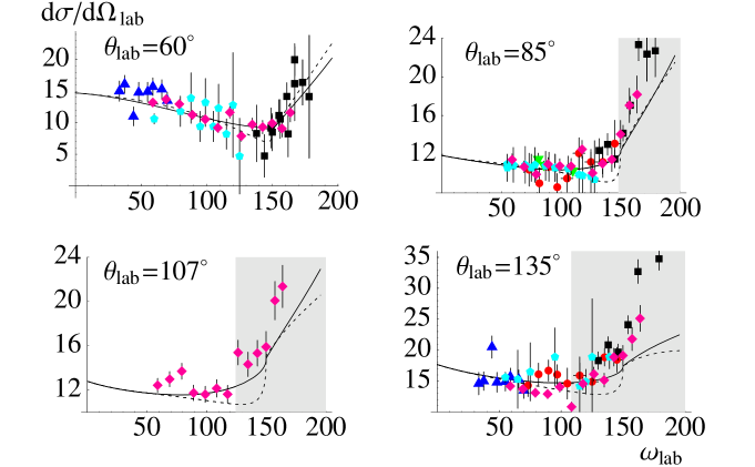
Figure 1: Results of the ${\cal O}(Q^{4})$ EFT best fit (solid line) to the differential cross sections for Compton scattering on the proton at four different angles, compared to the experimental data pdata ; fitting . (Symbols as in Ref. judith .) The grey area is the region excluded from the fit ($\omega,\sqrt{|t|}>200$ MeV). The dashed line is the ${\cal O}(Q^{3})$ prediction.

Thus the calculation of Ref. judith is not, strictly speaking, model independent: there is model input in the values used for $\alpha_{p}$ and $\beta_{p}$. Using the same amplitude but fitting the polarizabilities, very good fits of the proton data in the low-energy regime ($\omega,\sqrt{|t|}<200$ MeV) can be obtained. The central values for $\alpha_{p}$ and $\beta_{p}$ are similar to those employed in Ref. judith , but the uncertainty is larger:

$$\alpha_{p} = (12.1\pm 1.1)_{-0.5}^{+0.5}\times 10^{-4}\,{\rm fm}^{3},$$

$$\beta_{p} = (3.4\pm 1.1)_{-0.1}^{+0.1}\times 10^{-4}\,{\rm fm}^{3},$$ (2)

where statistical (1-$\sigma$) errors are inside the brackets, and an estimate of the contribution from higher-order terms is given outside. These numbers are based on varying the upper bound on which data are fit from 160 MeV to 200 MeV, and on estimates of the ${\cal O}(Q^{5})$ effect on $\gamma p$ scattering. A sample of the best-fit results is shown, together with data, in Fig. 1. The fit has $\chi^{2}/{\rm d.o.f.}=170/131$. These results are fully compatible with other extractions, though the central value of $\beta_{p}$ is somewhat higher PDG ; drechsel . They are also consistent with the values predicted in Ref. ulf1 ; bernard , where resonance saturation was used to estimate the ${\cal O}(Q^{4})$ short-distance contributions.

The values (2) can be compared with the recent re-evaluation of the Baldin Sum Rule by Olmos de León et al. pdata , which gives:

$$\alpha_{p}+\beta_{p}=13.8\pm 0.4.$$ (3)

This result overlaps the 1-$\sigma$ error ellipse of the fit (2), as shown in Fig. 2. Including the constraint (3) in our fit leads to values for $\alpha_{p}$ and $\beta_{p}$ consistent with (2), but with smaller statistical errors, namely:

$$\alpha_{p} = (11.0\pm 0.5\pm 0.2)_{-0.5}^{+0.5}\times 10^{-4}\,{\rm fm}^{3},$$

$$\beta_{p} = (2.8\pm 0.5\mp 0.2)_{-0.1}^{+0.1}\times 10^{-4}\,{\rm fm}^{3}.$$ (4)

In (4) we have left the systematic error unchanged, but have now included a second error inside the brackets, whose source is the error on the sum rule evaluation (3). The smaller overall statistical error in (4) is achieved at the expense of additional (reasonable) assumptions about the high-energy behaviour of hadronic amplitudes, and also by using higher-energy data on the total proton photo-absorption cross section, since these are the two ingredients entering the Baldin Sum Rule result for $\alpha_{p}+\beta_{p}$.

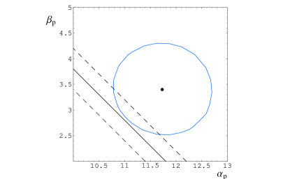
Figure 2: The 1-$\sigma$ error ellipse for our fit to the proton data with $\omega,\sqrt{|t|}<200$ MeV. Also shown is the band defined by the Baldin Sum Rule result (3). The units of $\alpha_{p}$ and $\beta_{p}$ are $10^{-4}~{}{\rm fm}^{3}$.

The amplitude for Compton scattering on a nuclear target can also be calculated in the EFT, although the unraveling of scales is more subtle when more than one nucleon is present bkreview . In the single-nucleon sector a typical intermediate state has an energy denominator of ${\cal O}(Q)$, but in multi-nucleon processes “reducible” intermediate states can have small energy denominators of ${\cal O}(Q^{2}/m_{N})$. The resulting infrared enhancement complicates the perturbative expansion weinberg . Furthermore, the very existence of nuclei implies a breakdown of perturbation theory; hence the leading two-nucleon interactions should be summed to all orders, thereby building up a nuclear wave function $|\psi\rangle$. In the case of Compton scattering at energies of ${\cal O}(m_{\pi})$, this is the only resummation necessary therestofus , and the full amplitude, $T$, can be written in terms of a kernel $K_{\gamma\gamma}$ which contains all irreducible (in the above sense) $\gamma NN\rightarrow\gamma NN$ graphs:

$$T=\langle\psi|K_{\gamma\gamma}|\psi\rangle.$$ (5)

The kernel can be calculated in $\chi$PT. Several other reactions involving deuterium have been successfully analyzed using analogous approaches bkreview . However, for Compton scattering at energies of ${\cal O}(m_{\pi}^{2}/m_{N})$ further resummations are necessary. In particular, such resummations restore the Thomson limit for Compton scattering from deuterium FT ; springer ; therestofus . In this energy regime it seems more appropriate to use a lower-energy EFT where pions have been integrated out BS ; GR00 .

At momentum transfers of ${\cal O}(m_{\pi})$, a formally-consistent power counting is emerging chiralexp which organizes the nuclear interactions that give rise to the wave function $|\psi\rangle$. This power counting is an improvement over Weinberg’s original proposal weinberg , which has led to fairly accurate wave functions bkreview . To the order we are working in the EFT, we require a deuteron wave function calculated to ${\cal O}(Q^{2})$ in the chiral expansion. We employ a wave function generated using the ${\cal O}(Q^{2})$ $\chi$PT potential of Ref. chipots . (The $\Lambda=600$ MeV wave function was chosen, but choosing $\Lambda=540$ MeV instead produces very similar results.) In order to test the consistency of our error estimates, we have also computed results with other “realistic” wave functions, such as that obtained from the Nijm93 OBE potential Nijm93 . Below we will quote results only for the ${\cal O}(Q^{2})$ wave function of Ref. chipots and for the Nijm93 wave function. The results for differential cross sections generated using $|\psi\rangle$’s obtained from other $NN$ potentials almost invariably lie between these two extremes.

Meanwhile, the kernel $K_{\gamma\gamma}$ is the sum of the single-nucleon Compton amplitude, in which one nucleon is a “spectator” to the Compton scattering, and “two-nucleon” contributions in which both nucleons are involved in the scattering of the photon. The amplitude for coherent Compton scattering on the deuteron was computed to ${\cal O}(Q^{3})$ in Ref. therestofus . There are no free parameters to this order. The corresponding cross section is in good agreement with the Illinois data lucas at 49 and 69 MeV, but under-predicts the SAL data SAL at 95 MeV. This calculation yields cross sections which agree well with the recent Lund data lund . It also agrees qualitatively with potential-model calculations of $\gamma d$ scattering potmods ; LL .

We have now extended our calculation to ${\cal O}(Q^{4})$. The calculation contains both single-nucleon and two-nucleon contributions. For the first class of diagrams, we employ the single-nucleon amplitude of Ref. judith . The amplitude given there must be boosted from the Breit frame to the $\gamma d$ center-of-mass frame, which is straightforward once the $\gamma p$ amplitude has been decomposed into six invariant functions multiplying structures that transform in well-defined ways under boosts therestofus ; usagain .

Less straightforward are technical issues associated with the fashion in which nucleon recoil is included in the $\gamma d$ scattering calculation. These occur because the heavy-baryon formulation of $\chi$PT employed in this work expands about the limit of static nucleons, with nucleon recoil treated as a perturbative correction. The first issue has to do with the treatment of the very-low-energy region, $\omega\sim m_{\pi}^{2}/M$. At these energies the nucleons inside the deuteron are not static on the time-scales relevant to Compton scattering, and so a resummation of nucleon-recoil corrections must be performed. Below we will invoke this resummation when we calculate $\gamma d$ scattering for these low photon energies. The second issue has to do with ensuring that particle-production cuts appear at the correct position. In the absence of nucleon recoil the channel $\gamma d\rightarrow\pi d$ will open at a position which is in error by an amount $m_{\pi}^{2}/(2M_{d})$. Since the opening of this channel can result in rapid variation of the Compton cross section with energy, this problem must be dealt with when we describe $\gamma p$ scattering for $\omega$ close to $m_{\pi}$ bernard ; judith . However, even at the highest energy for which Compton scattering on deuterium is calculated below, this small error in the position of the $\pi d$ cut is a relatively minor effect. We emphasize that these subtleties are artifacts which arise due to the fact that nucleon recoil is treated as a perturbation in the $\gamma$N amplitude we have employed here judith . Such a treatment is in accord with the usual practice in the chiral EFT known as heavy-baryon $\chi$PT, but a perturbative treatment of nucleon recoil in not mandatory in the EFT. Thus these two problems in no way represent true limitations of a chiral EFT of Compton scattering.

In addition, the two-nucleon diagrams at ${\cal O}(Q^{4})$ are added to the two-nucleon ${\cal O}(Q^{3})$ diagrams shown in Ref. therestofus . These ${\cal O}(Q^{3})$ graphs were generated by the leading chiral Lagrangian. In going to ${\cal O}(Q^{4})$ we include diagrams with one insertion from the sub-leading chiral Lagrangian. The coefficients of these vertices are essentially determined by relativistic invariance, and so these ${\cal O}(Q^{4})$ two-body effects are suppressed by $Q/m_{N}$. No unknown parameters occur in these graphs. However, two free parameters associated with the neutron polarizabilities do appear in the single-nucleon contribution: the shifts in the isoscalar polarizabilities from their ${\cal O}(Q^{3})$ values. Indeed, of all the additional graphs which enter our new, ${\cal O}(Q^{4})$, calculation only this effect from single-nucleon Compton scattering changes the cross section significantly. (Details can be found in Ref. usagain .)

We have fitted these two free parameters to the existing $\gamma d$ scattering data. As in the proton case, we impose a cutoff on the data that we fit when we extract $\alpha$ and $\beta$. With a cutoff of $\omega,\sqrt{|t|}<200$ MeV all of the 29 world data points lucas ; SAL ; lund are included. We also use a cutoff of 160 MeV, in which case all but the two backward-angle SAL points must be fitted. In both cases we float the experimental normalization for each experimental run within the quoted systematic error fitting , resulting in 22 (20) degrees of freedom for the fit usagain .

Using the wave function of Ref. chipots , we fit to data with $\omega,\sqrt{|t|}<160$ MeV. This produces the isoscalar nucleon polarizabilities and the $\chi^{2}$ per degree of freedom given in the first line of Table 1. The $\chi^{2}$ is unacceptably large. This is driven mainly by the 49 MeV data from Illinois, and occurs because, as discussed above, for $\omega\sim m_{\pi}^{2}/m_{N}$ further resummations are necessary in the EFT. Here we adopt the strategy of including the dominant contributions that need to be added to our standard ${\cal O}(Q^{4})$ result in this very-low-energy region in order to restore the Thomson limit for the $\gamma d$ amplitude therestofus . This yields the results on the second line of Table 1. An alternative strategy, namely dropping the 49 MeV data altogether, produces very similar central values for $\alpha_{N}$ and $\beta_{N}$.

Chiral	Wave	Very-low-energy	$\omega,\sqrt{|t|}$	$\alpha_{N}$	$\beta_{N}$	$\chi^{2}$/d.o.f.
order	function	resummation?		$(10^{-4}~{}{\rm fm}^{3})$	$(10^{-4}~{}{\rm fm}^{3})$
$Q^{4}$	NLO $\chi$PT	No	$200$ MeV	13.6	$0.1$	2.36
$Q^{4}$	NLO $\chi$PT	No	$160$ MeV	15.4	$-2.3$	1.95
$Q^{4}$	NLO $\chi$PT	Yes	$160$ MeV	13.0	$-1.8$	1.33
$Q^{4}$	Nijm93	Yes	$200$ MeV	16.9	$-2.7$	2.87

Table 1: Results from different $\chi$PT extractions of isoscalar nucleon polarizabilities from $\gamma d$ scattering data.

When the upper limit on which data is fitted is increased the central value of $\alpha_{N}-\beta_{N}$ changes markedly, with a slightly higher $\chi^{2}$/d.o.f. (third line of Table 1). Another key test involves examining the impact of the choice of deuteron wave function. The variability in the differential cross section due to the choice of wave function is $\sim 10$%. When the Nijm93 wave function is used the results are as shown in the fourth line of Table 1. The high $\chi^{2}$ is again due to a failure to reproduce the 49 MeV data—this time even with the very-low-energy contributions included. While the Nijm93 wave function is not consistent with $\chi$PT, it does have the correct long-distance behavior. Such sensitivity to the choice of $|\psi\rangle$ is worrisome and merits further study.

Putting these results together we conclude that our best fit, and error bars, for the isoscalar nucleon polarizabilities are:

$$\alpha_{N} = (13.0\pm 1.9)_{-1.5}^{+3.9}\times 10^{-4}\,{\rm fm}^{3},$$

$$\beta_{N} = (-1.8\pm 1.9)_{-0.9}^{+2.1}\times 10^{-4}\,{\rm fm}^{3}.$$ (6)

The statistical errors inside the brackets are obtained from the boundary of the 68% C.L. region. The errors outside the brackets reflect the arbitrariness as to which data are included, and which deuteron wave function is employed. The results for the best-fit EFT are shown in Fig. 3.

The results (6) differ from those given in the published version of this work allofus , since after publication we discovered two errors in our analysis of the $\gamma$d data lucas ; SAL ; lund . First, we mistakenly fitted the SAL data at a c.m. energy of 95 MeV, whereas we should have employed a lab energy of 94.5 MeV SAL . (A similar error that ultimately has a much smaller impact was made with the data from Lund lund .) This causes a relatively small change in the results for most of our fits, but it does increase the central value for $\alpha_{N}$ obtained with the Nijm93 deuteron wave function by $1.0\times 10^{-4}~{}{\rm fm}^{3}$ over the value quoted in the published version of Ref. allofus  . A larger effect occurs because there was an error in the program used to generate the $O(Q^{4})$ results presented for $\gamma$d scattering in Ref. allofus . This affects the $O(Q^{3})$ results by less than 1%. However, at $O(Q^{4})$ the omission of this factor modifies the interference between the spin-dependent pieces of the single-nucleon amplitude and the $O(Q^{4})$ two-body currents . Correcting this mistake increases the predicted cross sections by about 10-15% with respect to those published in Ref. allofus . We emphasize that neither of these mistakes affects any of the results for $\gamma$p scattering reported here and in the published version of Ref. allofus . For more details see Ref. usagain .

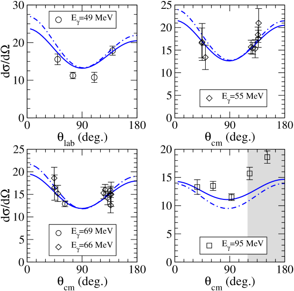
Figure 3: Results of the $O(Q^{4})$ EFT best fit to the (lab and c.m. as appropriate) differential cross sections for Compton scattering on deuterium at four different lab photon energies: 49, 55, 67, and 94.5 MeV. The data are from Illinois lucas (circles), Lund lund (diamonds) and SAL (squares) SAL . The error bars represent the quoted statistical (only) uncertainties of these measurements. The solid line is the $O(Q^{4})$ calculation with $\alpha_{N}=13.0\times 10^{-4}~{}{\rm fm}^{3}$, $\beta_{N}=-1.8\times 10^{-4}~{}{\rm fm}^{3}$. The gray area is the region excluded from the fit ($\omega,\sqrt{|t|}>160$ MeV). The dot-dashed line is the (parameter-free) $O(Q^{3})$ calculation.

Combining the revised numbers (6) with our results for $\alpha_{p}$ and $\beta_{p}$ we see that a wide range of neutron polarizabilities is consistent with a model-independent analysis of the current low-energy proton and coherent deuteron Compton data. Narrower ranges for the neutron polarizabilities can be obtained from this data at the expense of introducing model dependence. The values of $\alpha_{n}$ and $\beta_{n}$ extracted from data on the quasi-free process $\gamma d\rightarrow\gamma np$ using a theoretical model fall within this range quasidata . However, there is clear statistical evidence in these data sets for $\alpha_{n}$ being significantly larger than $\beta_{n}$: $\beta_{n}$ is consistent with zero within our large error bars. Also, the results presented here provide no evidence for significant isovector components in $\alpha$ and $\beta$.

In conclusion, we have determined nucleon polarizabilities from a model-independent fit to low-energy Compton scattering on the proton and the deuteron. Our results are consistent, within error bars, with the recent extraction of $\alpha_{N}\pm\beta_{N}$ from the Lund data using the detailed model of Levchuk and L’vov lund ; LL . (But see also the values found using the data of Refs. lucas ; SAL and this model SAL ; LL .). They are also consistent with the Baldin sum rule results for $\alpha_{p}+\beta_{p}$ and $\alpha_{n}+\beta_{n}$ baldin . The EFT can be improved by the introduction of an explicit $\Delta$-isobar field, a complete treatment of the very-low-energy region, and a better understanding of the dependence of the results on the choice of deuteron wave function. An EFT study of the quasi-free deuteron process is also an important future step.

- (1) B.R. Holstein, Comm. Nucl. Part. Phys. 20, 301 (1992).
- (2) The predictions of an EFT of QCD for scattering have been compared with cross-section data, for instance, in Ref. judith and in D. Babusci, G. Giordano and G. Matone, Phys. Rev. C 55, 1645 (1997). However, no extraction of proton polarizabilities was made in either paper. There is also recent work in which isoscalar nucleon polarizabilities are obtained via an EFT analysis of a (restricted) set of data GR00 . However, the authors of Ref. GR00 did not attempt an analysis of proton scattering in the low-energy EFT used in that work.
- (3) J.A. McGovern, Phys. Rev. C 63, 064608 (2001), see also nucl-th/0101057 v2.
- (4) S.R. Beane, M. Malheiro, D.R. Phillips, and U. van Kolck, Nucl. Phys. A 656, 367 (1999).
- (5) S.R. Beane, M. Malheiro, J.A. McGovern, D.R. Phillips, and U. van Kolck, arXiv:nucl-th/0403088, Nucl. Phys. A, in press.
- (6) Our definition of the polarizabilities is identical to that used in recent DR extractions - see D. Babusci, G. Giordano, A.I. L’vov, G. Matone and A.M. Nathan, Phys. Rev. C58, 1013 (1998). They are the leading terms in the expansion of the non-Born amplitudes.
- (7) P.S. Baranov et al., Sov. J. Nucl. Phys. 21, 355 (1975); F.J. Federspiel et al., Phys. Rev. Lett. 67, 1511 (1991); A. Ziegler et al., Phys. Lett. B 278, 34 (1992); E.L. Hallin et al., Phys. Rev. C 48, 1497 (1993); B.E. MacGibbon et al., Phys. Rev. C 52, 2097 (1995); V. Olmos de León et al., Eur. Phys. J. A 10, 207 (2001).
- (8) P.S. Baranov, A.I. L’vov, V.A. Petrun’kin, and L.N. Shtarkov, Phys. Part. Nucl. 32, 376 (2001).
- (9) M. Lucas, Ph.D. thesis, University of Illinois, unpublished (1994).
- (10) D.L. Hornidge et al., Phys. Rev. Lett. 84, 2334 (2000).
- (11) M. Lundin et al., nucl-ex/0204014.
- (12) N.R. Kolb et al., Phys. Rev. Lett. 85, 1388 (2000); K. Kossert et al., Phys. Rev. Lett. 88, 162301 (2002).
- (13) D.B. Kaplan, nucl-th/9506035; D.R. Phillips, Czech J. Phys. 52, B49 (2002).
- (14) V. Bernard, N. Kaiser, and U.-G. Meißner, Int. J. Mod. Phys. E4, 193 (1995).
- (15) P.F. Bedaque and U. van Kolck, Ann. Rev. Nucl. Part. Sci. 52, 339 (2002); S.R. Beane, P.F. Bedaque, W.C. Haxton, D.R. Phillips, and M.J. Savage, Encyclopedia of Analytic QCD, At the Frontier of Particle Physics, vol. 1, 133-269, edited by M. Shifman (World Scientific).
- (16) V. Bernard, N. Kaiser, and U.-G. Meißner, Nucl. Phys. B383, 442 (1992); V. Bernard, N. Kaiser, J. Kambor, and U.-G. Meißner, Nucl. Phys. B388, 315 (1992).
- (17) D.E. Groom et al. [Particle Data Group], Eur. Phys. J. C 15, 1 (2000).
- (18) D. Drechsel, B. Pasquini and M. Vanderhaeghen, hep-ph/0212124.
- (19) V. Bernard, N. Kaiser, U. G. Meissner and A. Schmidt, Z. Phys. A348, 317 (1993).
- (20) S. Weinberg, Phys. Lett. B 251, 288 (1990); Nucl. Phys. B 363, 3 (1991).
- (21) J.L. Friar and E.I. Tomusiak, Phys. Lett. B 122, 11 (1983).
- (22) J.W. Chen, H.W. Grießhammer, M.J. Savage, and R.P. Springer, Nucl. Phys. A 644, 245 (1998).
- (23) S.R. Beane and M.J. Savage, Nucl. Phys. A 694 511 (2001).
- (24) H.W. Grießhammer and G. Rupak, Phys. Lett. B 529, 57 (2002).
- (25) S.R. Beane, P.F. Bedaque, M.J. Savage, and U. van Kolck, Nucl. Phys. A 700, 377 (2002).
- (26) E. Epelbaum, W. Glöckle, and U.-G. Meißner, Nucl. Phys. A 671, 295 (2000).
- (27) V.G. Stoks, R.A. Klomp, C.P. Terheggen and J.J. de Swart, Phys. Rev. C 49, 2950 (1994). Our kernel is derived for low momenta, so we have applied an integration cutoff of 600 MeV when this wave function is used, so we can make a consistent comparison with our other results.
- (28) T. Wilbois, P. Wilhelm, and H. Arenhövel, Few-Body Syst. Suppl. 9, 263 (1995); J.J. Karakowski and G.A. Miller, Phys. Rev. C60, 014001 (1999);
- (29) M.I. Levchuk and A.I. L’vov, Nucl. Phys. A674, 449 (2000).
- (30) D. Babusci, G. Giordano, and G. Matone, Phys. Rev. C57, 291 (1998).
- (31) S. R. Beane, M. Malheiro, J. A. McGovern, D. R. Phillips and U. van Kolck, Phys. Lett. B 567, 200 (2003).