Periodic Orbits and Deformed Shell Structure

Abstract

Relationship between quantum shell structure and classical periodic orbits is briefly reviewed on the basis of semi-classical trace formula. Using the spheroidal cavity model, it is shown that three-dimensional periodic orbits, which are born out of bifurcation of planar orbits at large prolate deformations, generate the superdeformed shell structure.

Introduction

Existence of superdeformed (SD) nuclei is often explained in terms of the SD magic numbers for the harmonic-oscillator (HO) potential with axis ratio 2:1. It appears, however, that we need a more general explanation not restricted to the HO potential, since, up to now, more than 200 SD bands have been found in various regions of nuclear chart and their shapes in general deviates from the 2:1 shape to some extent. In this talk, we shall discuss the mechanism how and the reason why the SD shell structure emerges. The major tool for this purpose is the trace formula, which is the central formula in the semiclassical periodic-orbit (PO) theory and provides a link between quantum shell structure and classical periodic orbits in the mean field. Here, shell structure is defined as regular oscillation in the single-particle level density coarse-grained to a certain energy resolution. An example of coarse-graining for the well-known axially symmetric HO model is displayed in Fig. 1.

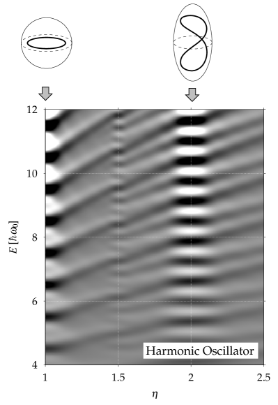
Figure 1: Oscillating level density as a function of axis ratio $\eta$ for the axially symmetric HO potential. Bright and dark regions correspond to high and low level densities, respectively. The 3D periodic orbits exist only at the 2:1 shape.

In this talk, we discuss the spheroidal cavity model, since, in contrast to the HO model, this model is very rich in periodic orbits; it is an ideal model for exhibiting the presence of various kinds of periodic orbit and their bifurcations. We present both Fourier transforms of quantum spectra and semiclassical calculations based on the PO theory, and identify classical periodic orbits responsible for emergence of the SD shell structure. The result clearly shows that three-dimensional (3D) periodic orbits, that are absent in spherical and normal deformed systems and are born out of bifurcations of planar orbits, generate a new shell structure at large prolate deformations, which may be called “the SD shell structure.” They continue to exist for a wide range of deformation, once they are born.

The PO theory provides a basic tool to get a deeper understanding of microscopic origin of symmetry breaking in the mean field. It sheds light, in addition to the stability of the SD nuclei, on the reason of prolate dominance in normal deformed nuclei, on the origin of left-right asymmetric shapes, etc. It is useful for finite many-Fermion systems covering such different areas as nuclei, metallic clusters, quantum dots, etc. In this talk, we shall also touch upon such applications of the PO theory.

Level Bunching and Trace Formula

For the axially symmetric HO potential, the following two conditions coincide:

1. Axis ratio    $\langle x^{2}\rangle:\langle z^{2}\rangle=1:2$

2. Frequency ratio    $\omega_{x}:\omega_{z}=2:1\,,$

but they are different in general. Condition 2) is nothing but the PO condition, and possesses a more general significance than condition 1). We can examine this point as follows. For any integrable Hamiltonian system, we can introduce action and angle variables $(\bm{I},\bm{\theta})$ which satisfy the canonical equations of motion,

$$\dot{\bm{\theta}}=\frac{\partial H}{\partial\bm{I}}=\bm{\omega}(\bm{I}),$$ (1)

and the energy $E$ can be quantized by the EBK (Einstein-Brillouin-Keller) quantization condition:

$$E_{\bm{n}}=H(\bm{I})~{}~{}~{}~{}~{}{\rm with}~{}~{}~{}\bm{I}=\hbar\,(\bm{n}+{\textstyle\frac{1}{4}}\bm{\alpha}),$$ (2)

where $\bm{n}$ represents a set of quantum numbers, $\bm{n}=(n_{1},n_{2},n_{3})$ with $n_{i}=0,1,2,\cdots$, and $\bm{\alpha}$ the Maslov indices. We see that level degeneracy occurs when

$$E_{\bm{n}+\Delta\bm{n}}-E_{\bm{n}} = H(\bm{I}+\Delta\bm{I})-H(\bm{I})$$ (3)

$$\simeq \frac{\partial H}{\partial\bm{I}}\Delta\bm{I}$$

$$= \hbar\bm{\omega}\cdot\Delta\bm{n}$$

$$= \hbar\omega_{1}\Delta n_{1}+\hbar\omega_{2}\Delta n_{2}+\hbar\omega_{3}\Delta n_{3}$$

$$= 0,$$

i.e., when $\omega_{1}:\omega_{2}:\omega_{3}$ are in rational ratios. This is just the condition for the classical orbit to be periodic, and discussed in detail in the textbook of Bohr and Mottelsonbor75 .

On the basis of the semiclassical PO theory, we can examine, in a more general way, the decisive role of periodic orbits as origin of level bunching. According to this theory (see, e.g., bra97a for a review), the level density $g(E)$ is given by a sum of the average part $\bar{g}(E)$ and the oscillation part $\delta g(E)$ as

$$g(E) = \sum_{n}\delta(E-E_{n})$$ (4)

$$\simeq \bar{g}(E)+\delta g(E)$$

$$= \bar{g}(E)+\sum_{\alpha}A_{\alpha}\cos\left(\frac{1}{\hbar}S_{\alpha}(E)-\frac{\pi}{2}\mu_{\alpha}\right),$$

where $S_{\alpha}(E)$ denotes the action of the periodic orbit $\alpha$, and $\mu_{\alpha}$ is a phase related with the Maslov index. This equation is called “trace formula” and provides a link between quantum shell structure and classical periodic orbits in the mean field. There is a complementarity between the energy resolution and periods of classical orbits, so that, for the purpose of understanding the origin of regular oscillation patterns in the smoothed single-particle level density (shell structure), we need only short orbits in the sum over $\alpha$.

Figure 2: Oscillating level density as a function of axis ratio $\eta$ for the WS potential without the spin-orbit term. Bright and dark regions correspond to high and low level densities, respectively. The calculation was done following the procedure described on p. 593 of Ref. bor75 .

Figure 3: Oscillating level density as a function of axis ratio $\eta$ for the WS potential. Bright and dark regions correspond to high and low level densities, respectively. Here, the spin-orbit term with $v_{ls}=-0.12$ is added to the Hamiltonian used in Fig. 3.

Periodic Orbits and Shell Structure in the Cavity Model

Let us consider the cavity model, which may be regarded as a simplified model of Woods-Saxon potential for heavy nuclei. In fact their basic patterns of shell structure are similar with each other. Certainly, the spin-orbit term shifts the magic numbers, but it does not destroy the valley-ridge structure discussed below. One can confirm these points by comparing Figs. 3, 3 and 4.

Role of periodic orbits for shell structure in this model was originally studied by Balian and Blochbal72 , and has been discussed in the investigations of

1. the reason of prolate dominance in nuclear shape str77 ; arv87 ; fri90

2. the supershell effects in metallic clustersnis90

3. the origin of left-right asymmetric shapesbra97b ; sug98 ,   etc.

For cavity models, the energy and the momentum are simply related as

$$E=\bm{p}^{2}/2m,\qquad\bm{p}=\hbar\bm{k},$$ (5)

and the action integral is proportional to the length $L_{\alpha}$,

$$S_{\alpha}=\oint_{\alpha}\bm{p}\cdot d\bm{x}=\hbar kL_{\alpha}.$$ (6)

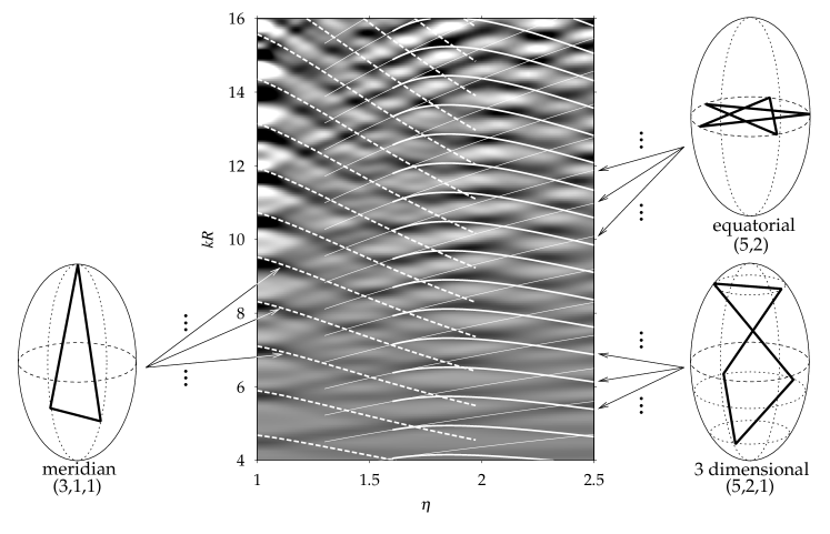
Figure 4: Ridge-valley structure in the oscillating level density for the spheroidal cavity model. Bright and dark regions correspond to high (ridge) and low (valley) values of the oscillating level density, respectively. Constant action lines running along valleys are shown for typical periodic orbits by dashed, thin-solid, and thick-solid curves. Note that they are indicated as representatives of the meridian-plane orbits, the equatorial-plane orbits, and the 3D orbits, respectively: There are several families of periodic orbits with similar lengths, and constant-action lines of them also behave in the same way as those shown here, see Refs. str77 and ari98 for details.

Accordingly, the trace formula for the level density can be written as

$$g(k)\simeq\bar{g}(k)+\sum_{\alpha}A_{\alpha}\cos\left(kL_{\alpha}-\frac{\pi}{2}\mu_{\alpha}\right).$$ (7)

It can be easily confirmed that only short orbits contribute to the level density coarse-grained in energy. Let us Fourier transform the level density

$$F(L) = \int dke^{ikL}g(k)$$ (8)

$$\simeq \sum_{\alpha}\tilde{A}_{\alpha}\delta(L-L_{\alpha}).$$

This equation indicates that peaks will show up at lengths $L_{\alpha}$ of periodic orbits $\alpha$, which may be called “length spectrum”. Now, the orbit lengths change when the deformation parameter $\eta$ varies. Let us then consider the oscillating level density as a function of $\eta$,

$$\delta g(k,\eta)\simeq\sum_{\alpha}A_{\alpha}(k,\eta)\cos\left(kL_{\alpha}(\eta)-\frac{\pi}{2}\mu_{\alpha}\right).$$ (9)

From this formula, we see that, if a few orbits dominate in the sum, the valley-ridge structure on the $(k,\eta)$ plane will be determined by the constant action lines,

$$kL_{\alpha}(\eta)={\rm const},$$ (10)

of these dominant orbitsstr77 ; ari98 . In fact, we see in Fig. 4 that the valley-ridge structure is well explained in terms of three kinds of short periodic orbit.

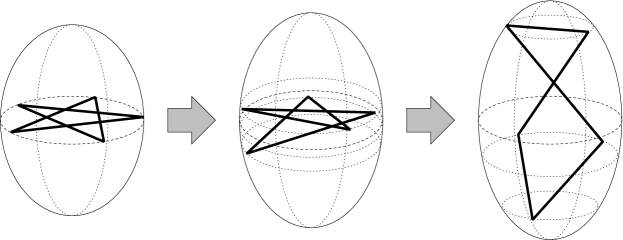
Figure 5: Birth of a butterfly shaped orbit from the short diameter through bifurcation at $\eta=\sqrt{2}$ on the meridian plane. This figure illustrates a representative orbit among a continuous family of orbits possessing the same length.

Figure 6: Birth of a 3D orbit from the star-shaped orbit on the equatorial plane through bifurcation at $\eta\simeq 1.62$. This figure illustrates a representative orbit among a continuous family of orbits possessing the same length.

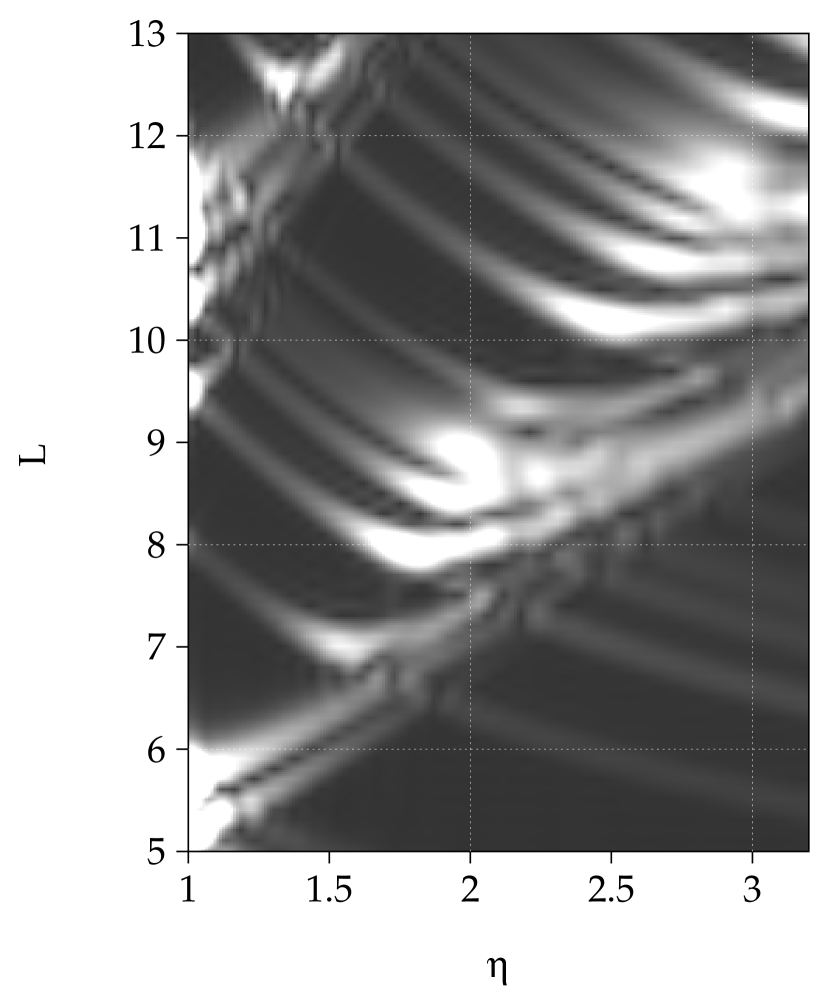
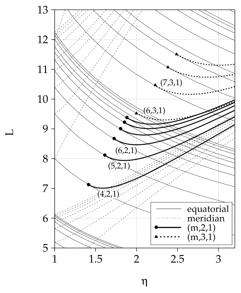
Figure 7: Left-hand part: Absolute values of the Fourier amplitudes, $|F(L,\eta)|$, of the level density, drawn as a map on the $(L,\eta)$ plane. Brightness is proportional to the magnitude. Right-hand part: Lengths of various classical orbits as functions of axis ratio $\eta$. The 3D orbits responsible for the SD shell structure are denoted as (4,2,1), (5,2,1), (6,2,1), etc., and their lengths are plotted by thick-solid curves, while those of the equatorial-plane orbits and of the meridian-plane orbits are plotted by thin-solid and dashed curves, respectively. @The bifurcation points of the 3D orbits of interest are indicated by filled circles. (Filled triangles indicate bifurcation points of 3D orbits responsible for hyperdeformed shell structure not discussed here.) See Refs. ari98 and mag02 for details.

Figure 8: Comparison between the oscillating level densities evaluated by the semiclassical trace formula (dotted lines denoted ISPM) and those obtained by quantum mechanics (solid lines denoted Quantum). They are plotted for several values of $\eta$ as function of $kR$, where $R$ denotes the radius of the cavity in the spherical limit (the volume of cavity is conserved during variation of $\eta$).

Bifurcations

As illustrated in Figs. 6 and 6, when the axis ratio $\eta$ of the spheroidal cavity reaches $\sqrt{2}$, the butterfly-shaped planar orbits emerge on the meridian plane through bifurcations of the linear orbit along the short diameter. When $\eta$ further increases, 3D orbits emerge at $\eta\simeq 1.62$ through bifurcation of the five-point star shaped orbits on the equatorial plane. Likewise, other 3D orbits appear at $\eta=\sqrt{3}$ through bifurcation of second repetitions of the triangular orbits on the equatorial plane, …, etc. Note that the figure illustrates representative orbits only. In fact, each $\alpha$ in the trace formula (9) represents a continuous family of orbits with the same topology possessing the same values of action (length). In contrast to the HO potential, these 3D orbits continue to exist, once they appear through the bifurcations.

Peaks in the Fourier transform (8) of the level density will follow the variations of orbit lengths $L_{\alpha}$ with $\eta$. Thus, we can draw a map of the Fourier amplitudes on the $(L,\eta)$ plane,

$$F(L,\eta)=\sum_{\alpha}\tilde{A}_{\alpha}\delta(L-L_{\alpha}(\eta)).$$ (11)

In Fig. 7, the Fourier amplitudes are compared with lengths of classical periodic orbits. This figure exhibits a beautiful quantum-classical correspondence. Furthermore, by comparing the bright regions in the left-side figure with the bifurcation points indicated in the right-side figure, we find significant enhancement of the shell structure amplitudes just on the right-hand side of the bifurcation points.

Unfortunately, the amplitude $A_{\alpha}(k,\eta)$ in the trace formula (9) diverges at the critical point of deformation $\eta$ where the orbit bifurcation takes place. This is because the stationary phase approximation used in the standard semiclassical PO theory breaks down there. Thus, the standard trace formula is unable to describe the enhancement phenomena seen in Fig. 7. To overcome this difficulty, in recent years, we have developed a new semiclassical approximation scheme, called an improved stationary phase approximation, and derived a new trace formula free from such divergencemag99 ; mag01 ; mag02 . A numerical example obtained by this approach is presented in Fig. 8. We see that the basic pattern of oscillation in the quantum level density at large deformation is nicely reproduced by the semiclassical calculation using the new trace formula. In this way, we have confirmedari98 ; mag01 ; mag02 that, in the region of large prolate deformation with axis ratio $\eta\geq 1.62$ (which corresponds to the ordinary deformation parameter $\delta\geq 0.44$), the major pattern of the oscillating level density is determined by contributions from the bifurcated 3D orbits.

Conclusion

The 3D periodic orbits generate a new shell structure at large prolate deformations. We may call this shell structure “SD shell structure.” These 3D orbits are born out of bifurcations of planar orbits in the equatorial plane, and they play dominant roles immediately after the bifurcations. Thus, the SD shell structure is a beautiful example of emergence of new structure through bifurcation, and may be regarded as quantum manifestation of classical bifurcation.

References

- (1) Bohr A. and Mottelson B., Nuclear Structure, vol. 2 (Benjamin, 1975) p.578.
- (2) Brack M. and Bhaduri R.K., Semiclassical Physics, (Addison-Wesley, Reading, 1997).
- (3) Balian R. and Bloch C., Ann. Phys. 69, 76(1972).
- (4) Strutinsky V.M., Magner A.G., Ofengenden S.R., and Døssing T., Z. Phys. A283, 269(1977).
- (5) Arvieu R., Brut F., Carbonell J., and Touchard J., Phys. Rev. A35, 2389(1987).
- (6) Frisk H., Nucl. Phys. A511, 309(1990).
- (7) Nishioka H., Hansen K., and Mottelson B.R., Phys. Rev. B42, 9377(1990).
- (8) Brack M., Reimann S.M., and Sieber M., Phys. Rev. Lett. 79, 1817(1997).
- (9) Sugita A., Arita K., and Matsuyanagi K., Prog. Theor. Phys. 100, 597(1998).
- (10) Arita K., Sugita A., and Matsuyanagi K., Prog. Theor. Phys. 100, 1223(1998).
- (11) Magner A.G., Fedotkin S.N., Arita K., Matsuyanagi K., Misu T., Schachner T., and Brack M., Prog. Theor. Phys. 102, 551(1999).
- (12) Magner A.G., Fedotkin S.N., Arita K., Matsuyanagi K., and Brack M., Phys. Rev. E63, 065201(R)(2001).
- (13) Magner A.G., Arita K., Fedotkin S.N., and Matsuyanagi K., Prog. Theor. Phys. to be published, arXiv:nlin.SI/0208005.