Theory of the Trojan-Horse Method

Abstract

The Trojan-Horse method is an indirect approach to determine the energy dependence of S-factors of astrophysically relevant two-body reactions. This is accomplished by studying closely related three-body reactions under quasi-free scattering conditions. The basic theory of the Trojan-Horse method is developed starting from a post-form distorted wave Born approximation of the T-matrix element. In the surface approximation the cross section of the three-body reaction can be related to the S-matrix elements of the two-body reaction. The essential feature of the Trojan-Horse method is the effective suppression of the Coulomb barrier at low energies for the astrophysical reaction leading to finite cross sections at the threshold of the two-body reaction. In a modified plane wave approximation the relation between the two-body and three-body cross sections becomes very transparent. The appearing Trojan-Horse integrals are studied in detail.

…$\kappa\epsilon\kappa\alpha\lambda\upsilon\mu\mu\epsilon\nu o\iota$ $\iota\pi\pi\omega$. Homer

I Introduction

Nuclear reaction rates are an indispensable ingredient of many astrophysical models. They have to be known with sufficient accuracy in order to understand quantitatively the evolution of the universe, stars and other objects in the cosmos Rol88 ; Thi01 ; Rol01 . Ideally, reaction cross sections are directly measured in the laboratory. But, with few exceptions and despite many experimental efforts, the relevant low energy range cannot be reached in direct experiments LUN02 ; Bon99 ; Jun98 . Cross sections for reactions with charged particles rapidly become very small with decreasing energy of the colliding nuclei due to the repulsive Coulomb interaction. Extrapolations of the cross section $\sigma(E)$ to low energies from results at higher energies accessible to experiments are often needed. This is accomplished with the help of the astrophysical S-factor

$$S(E)=\sigma(E)\>E\>\exp(2\pi\eta)$$ (1)

where $E$ is the c.m. energy and $\eta=Z_{1}Z_{2}e^{2}/(\hbar v)$ is the Sommerfeld parameter which depends on the charge numbers $Z_{1}$, $Z_{2}$ of the colliding nuclei and their relative velocity $v$ in the entrance channel. The S-factor shows a much weaker energy dependence than the cross section $\sigma(E)$ because the main effect of the penetrability through the Coulomb barrier is compensated by the increase of the exponential factor. The extrapolation process introduces uncertainties and important contributions to the cross sections, like resonances, can be missed. Additionally, direct laboratory experiments are affected by electron screening, which effectively reduces the Coulomb barrier between the nuclei and enhances the measured laboratory cross section Ass87 ; Sho93 ; Lio01 . A correction has to be applied to obtain the cross section for bare nuclei. This effect does not seem to be completely understood yet and independent information on low energy cross sections is valuable in order to develop a quantitative description of electron screening. In astrophysical applications one has, in addition, to account for the screening under stellar conditions.

In recent years several indirect methods have been developed to extract cross sections relevant to astrophysics from other types of experiments. In these alternative approaches the astrophysical relevant two-body reaction is generally replaced by a suitably chosen three-body reaction. The relation between the reactions is established with the help of nuclear reaction theories. Without doubt, this process will introduce some uncertainties, but valuable information on the astrophysical reaction can be obtained. Also, the errors are independent from that of the direct approach. Of course, the indirect methods have to be validated by studying well known reactions before firm conclusions can be drawn from indirect experiments in cases where direct measurements are not feasible; see also the minireview Aus02 .

The Coulomb dissociation method has become a valuable tool for extracting low-energy cross sections of radiative capture reactions $a(b,\gamma)c$ by studying the inverse process of photo dissociation $c(\gamma,b)a$ Bau94 . Instead of using real photons, the Coulomb field of a highly charged target $X$ acts as a source of virtual photons during a scattering process which leads to the breakup reaction $X(c,ab)X$ with three particles in the final state. Due to the high flux of virtual photons, cross sections at the small relevant energies in the two-body system are strongly enhanced as compared to the capture reaction. Another approach is the ANC method that tries to extract the asymptotic normalization coefficient of a nuclear ground state wave function by studying various combinations of transfer reactions involving this nucleus at low energies Azh01 ; Xu94 . The coefficient can be used to determine theoretically the astrophysical S-factor for radiative capture reactions at zero energy. However, these indirect approaches are limited to astrophysically relevant reactions where a photon is involved.

The observation of a similarity between cross sections for two-body and closely related three-body reactions under certain kinematical conditions Fuc71 led to the introduction of the Trojan-Horse method (THM) Bau86 , see also Bau84 ; Bau76 . The aim of the THM is to extract the cross section of an astrophysically relevant two-body reaction

$$A+x\to C+c$$ (2)

from a suitably chosen reaction

$$A+a\to C+c+b$$ (3)

with three particles in the final state assuming that the Trojan Horse $a$ is composed predominantly of clusters $x$ and $b$. The kinematical conditions are chosen such that the momentum transfer to the nucleus $b$ is small during the reaction. Therefore $b$ can be considered as a spectator to the reaction of $A$ and $x$. This process is often referred to as a quasi-free scattering. In a selected part of the available three-body phase space it is known to dominate over other reaction mechanism like sequential breakup processes. In the past quasi-free scattering has been used to extract information on momentum distributions of the nucleus $a$, i.e. the ground state wave function in momentum space, employing a plane-wave impulse approximation (PWIA) in the theoretical description Jai70 . In this approach the cross section of reaction (3) factorizes into a kinematical factor, the ground state momentum distribution of nucleus $a$ and an off-shell cross section of reaction (2) that is assumed to be known. On the other hand the two-body cross section can be extracted from the cross section of reaction (3) if the momentum distribution of the Trojan Horse $a$ is known with sufficient accuracy and a relation between the off-shell and on-shell two-body cross sections can be established. The selection of different spectators $b$ and thus Trojan Horses $a$ allows additional checks of the underlying assumptions of the method.

Unlike the Coulomb dissociation method and the ANC method which are limited to radiative processes, the THM can be applied to reactions where no photon is involved. The essential feature of the THM is the actual suppression of the Coulomb barrier in the cross section of the two-body reaction. The cross section of the three-body reaction is not reduced when the c.m. energy in the $A+x$ system approaches zero as in reaction (2). The energy in the entrance channel of (3) can be around or above the Coulomb barrier and effects from electron screening are negligible. Nevertheless, very small energies in the reaction (2) can be reached.

The feasibility of the THM was studied in several experiments involving various reactions during the last years Mus01 ; Spi01 ; Che96 ; Lat01 ; Ali00 ; Spi99 ; Cal97 ; Spi00 ; Pel00 . In earlier evaluations of the experiments some simplifying assumptions were made in the theoretical description. The off-shell two-body cross section as appearing in the PWIA was considered as the bare nuclear cross section. It was converted to the on-shell two-body cross section by correcting for the Coulomb penetration in a heuristic approximation. Basic considerations for the theoretical description of the THM were developed in Typ00 but the deduced relation between the cross sections for reactions (2) and (3) were not directly applicable to the experiments.

In this paper the theory of the THM is developed in certain approximations that allow to establish a simple connection between the cross sections of the three-body and two-body reactions. In Section II the reaction theory is formulated and the relation of the T-matrix element of the three-body reaction with the S-matrix elements of the two-body reaction is found. In connection with a plane wave approximation, fundamental TH integrals appear that are discussed in Section III. In the following two sections expressions for scattering amplitudes and cross sections are derived for spinless particles and then for the general case of particles with spin. The TH Coulomb scattering amplitude that is relevant in the indirect study of elastic scattering processes is treated in Section VI. Kinematical conditions, the energy dependence of cross sections and applications ot the THM are discussed in Section VII. A summary and an outlook are presented in the last Section. Details of the analytical calculations are given in the Appendices. The evaluation of actual Trojan-Horse experiments with the present theory is beyond the scope of this paper und is subject to a detailed treatment in separate studies.

II Reaction Theory

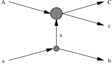
Figure 1: Transfer of particle $x$ in the Trojan-Horse reaction (3).

In the three-body reaction (3) the particle $x$ is transferred from the Trojan Horse $a$ to the nucleus $A$ leading to the $C+c$ final state with the spectator $b$ of the Trojan Horse remaining, see Fig. 1. This reaction can be considered as a transfer to the continuum, where the inelastic reaction $A+x\to C+c$ can happen in addition to the elastic $A+x$ scattering. It is customary to describe such a direct reaction, i.e. $A+a\to C+c+b$, with the help of a distorted wave Born approximation. It is not required in the theoretical approach that $A+x\neq C+c$; elastic scattering processes in the two-body system can be treated in the formalism, too. Effects from the antisymmetrization of the wave functions will be neglected in the present treatment; they are expected to be small.

II.1 Coordinate Systems and Cross Sections

In a three-body system various sets of Jacobi coordinates are used to specify the positions of the particles. In the theoretical description we encounter the sets

$$\vec{r}_{xb}=\vec{r}_{x}-\vec{r}_{b}\>,\qquad\vec{r}_{Aa}=\vec{r}_{A}-\vec{r}_{a}=\vec{r}_{A}-\frac{m_{x}\vec{r}_{x}+m_{b}\vec{r}_{b}}{m_{x}+m_{b}}$$ (4)

in the initial partition and

$$\vec{r}_{Cc}=\vec{r}_{C}-\vec{r}_{c}\>,\qquad\vec{r}_{Bb}=\vec{r}_{B}-\vec{r}_{b}=\frac{m_{C}\vec{r}_{C}+m_{c}\vec{r}_{c}}{m_{C}+m_{c}}-\vec{r}_{b}$$ (5)

in the final partition. The symbol $B$ denotes the $C+c=A+x$ system. The coordinate vectors are shown in Fig. 2. The corresponding relative momenta and wave vectors are given by

$$\vec{p}_{ij}=\hbar\vec{k}_{ij}=\frac{m_{j}\vec{p}_{i}-m_{i}\vec{p}_{j}}{m_{i}+m_{j}}$$ (6)

for nuclei $i$ and $j$ with masses $m_{i},m_{j}$ and momenta $\vec{p}_{i},\vec{p}_{j}$ in the laboratory system, respectively. With the help of the kinetic energies

$$E_{ij}=\frac{p_{ij}^{2}}{2\mu_{ij}}$$ (7)

where the reduced masses

$$\mu_{ij}=\frac{m_{i}m_{j}}{m_{i}+m_{j}}$$ (8)

appear, energy conservation in the two-body reaction (2) can be expressed as

$$E_{Ax}=E_{Cc}-Q_{2}$$ (9)

with the Q-value

$$Q_{2}=(m_{A}+m_{x}-m_{C}-m_{c})c^{2}$$ (10)

and similarly

$$E_{Aa}=E_{Cc}+E_{Bb}-Q_{3}=E_{Ax}+E_{Bb}+Q_{2}-Q_{3}$$ (11)

with

$$Q_{3}=(m_{A}+m_{a}-m_{C}-m_{c}-m_{b})c^{2}$$ (12)

in case of the three-body reaction.

Figure 2: Coordinate vectors in the initial and final partitions of the Trojan-Horse reaction (3).

The general cross section for reaction (3) with three particles in the final state depends on the choice of the independent variables and the reference system. In the c.m. system the energy $E_{Cc}$ and the directions of the Jacobi momenta $\vec{p}_{Bb}$ and $\vec{p}_{Cc}$ completely specify the kinematical conditions for a given projectile energy. Then the differential cross section takes the form

$$\frac{d^{3}\sigma}{dE_{Cc}d\Omega_{Cc}d\Omega_{Bb}}=K_{\rm cm}\left|T_{fi}(\vec{k}_{Cc},\vec{k}_{Bb};\vec{k}_{Aa})\right|^{2}$$ (13)

with the c.m. kinematical factor

$$K_{\rm cm}=\frac{\mu_{Aa}\mu_{Bb}\mu_{Cc}}{(2\pi)^{5}\hbar^{7}}\frac{p_{Bb}p_{Cc}}{p_{Aa}}$$ (14)

and the T-matrix element $T_{fi}$. In an actual experiment, the particles $C$ and $c$ are usually detected in the laboratory system and it is more convenient to use

$$\frac{d^{3}\sigma}{dE_{C}d\Omega_{C}d\Omega_{c}}=K_{\rm lab}\left|T_{fi}(\vec{k}_{Cc},\vec{k}_{Bb};\vec{k}_{Aa})\right|^{2}$$ (15)

with the kinematical factor

$$K_{\rm lab}=\frac{\mu_{Aa}m_{C}}{(2\pi)^{5}\hbar^{7}}\frac{p_{C}p_{c}^{2}}{p_{Aa}}\left[\left(\frac{\vec{p}_{Bb}}{\mu_{Bb}}-\frac{\vec{p}_{Cc}}{m_{c}}\right)\cdot\frac{\vec{p}_{c}}{p_{c}}\right]^{-1}\>.$$ (16)

The laboratory differential cross section depends on the scattering angles of the nuclei $C$ and $c$ and the energy $E_{C}$. Again, these quantities, together with the beam energy, specify the kinematical conditions completely. The nuclei $A$ and $a$ can be projectile and target or vice versa. In case of particles with spin appropriate averages over initial states and sums over final states have to be considered.

II.2 Approximations of the T-Matrix Element

The T-matrix element $T_{fi}$ in (13) and (15) contains all the essential information relevant to the scattering process. It has to be calculated in a suitable approximation that allows to find the connection to the cross section of the astrophysical relevant reaction (2).

The Trojan-Horse reaction (3) has the form of a usual two-body reaction

$$A+a\to B+b$$ (17)

if the $C+c$ system is considered as an excited state of the compound system $B$. The exact T-matrix element for this reaction is given in the post-form description by

$$T_{fi}=\langle\exp\left(i\vec{k}_{Bb}\cdot\vec{r}_{Bb}\right)\phi_{B}\phi_{b}|V_{Bb}|\Psi^{(+)}_{Aa}(\vec{k}_{Aa},\vec{r}_{Aa})\rangle$$ (18)

with the exact scatttering wave function $\Psi^{(+)}_{Aa}(\vec{k}_{Aa},\vec{r}_{Aa})$ in the initial state and the potential $V_{Bb}$ between $B$ and $b$ in the final state New66 . The wavefunction $\phi_{i}$ of a nucleus $i$ depends only on internal coordinates which are not given explicitly. The relative motion of $B$ and $b$ is described by a plane wave with momentum $\hbar\vec{k}_{Bb}$. Applying the Gell-Mann Goldberger transformation Gel53 , the T-matrix element (18) assumes the form

$$T_{fi}=\langle\chi^{(-)}_{Bb}(\vec{k}_{Bb},\vec{r}_{Bb})\phi_{B}\phi_{b}|V_{Bb}-U_{Bb}|\Psi^{(+)}_{Aa}(\vec{k}_{Aa},\vec{r}_{Aa})\rangle$$ (19)

which is still an exact relation. For a detailed derivation see Typ00 . Here, $\chi^{(-)}_{Bb}(\vec{k}_{Bb},\vec{r}_{Bb})$ is a distorted wave for the $B-b$ relative motion generated by a suitably chosen optical potential $U_{Bb}$ that only depends on $\vec{r}_{Bb}$ but not on internal coordinates in contrast to $V_{Bb}$. In the THM the wave function $\phi_{B}$ does not describe a bound state but a complete scattering state

$$\phi_{B}=\Psi^{(-)}_{Cc}(\vec{k}_{Cc},\vec{r}_{Cc})$$ (20)

since the system $B=C+c$ is in the continuum.

In the post-form distorted-wave Born approximation (DWBA) the T-matrix element (19) is replaced by

$$T_{fi}^{DWBA}(\vec{k}_{Cc},\vec{k}_{Bb};\vec{k}_{Aa})=\langle\chi^{(-)}_{Bb}(\vec{k}_{Bb},\vec{r}_{Bb})\Psi^{(-)}_{Cc}(\vec{k}_{Cc},\vec{r}_{Cc})\phi_{b}|V_{xb}|\chi^{(+)}_{Aa}(\vec{k}_{Aa},\vec{r}_{Aa})\phi_{A}\phi_{a}\rangle$$ (21)

where the exact wave function $\Psi^{(+)}_{Aa}(\vec{k}_{Aa},\vec{r}_{Aa})$ is replaced by a distorted wave $\chi^{(+)}_{Aa}(\vec{k}_{Aa},\vec{r}_{Aa})$ for the $A-a$ relative motion. Additionally, the potential $V_{Bb}-U_{Bb}$ is approximated by $V_{xb}$ Typ00 ; Aus70 . This is the usual starting point of T-matrix calculations for direct transfer reactions.

In the next step, the so-called surface approximation is applied which is essential to the THM. For small distances between the colliding nuclei the optical potentials are usually strongly absorptive and only reactions at the surface of the nuclei contribute significantly to the matrix element. Therefore the full scattering wave function $\Psi^{(-)}_{Cc}(\vec{k}_{Cc},\vec{r}_{Cc})$ can be replaced by its asymptotic form for radii larger than a suitably chosen cutoff radius $R$ that is larger than the range of the nuclear potential. It is typically in the range of the sum of the radii of the two colliding nuclei. The interior part of $\Psi^{(-)}_{Cc}(\vec{k}_{Cc},\vec{r}_{Cc})$ is set to zero. The validity of the surface approximation was checked in Kas82 ; it was found to be quite good for the (d,p) reaction at $E_{d}=26$ MeV. The asymptotic form of the scattering wave function for $r_{\alpha}>R$, where $\alpha=Ax,Cc,\dots$ is a possible partition of the system $B$, is given by

$$\Psi^{(\pm)}_{Cc,{\rm asym}}(\vec{k}_{Cc},\vec{r}_{Cc})=\frac{4\pi}{k_{Cc}}\sum_{\alpha}\sum_{lm}\frac{\xi_{l}^{(\pm)}(\alpha)}{r_{\alpha}}i^{l}Y_{lm}(\hat{r}_{\alpha})Y_{lm}^{\ast}(\hat{k}_{Cc})\phi_{\alpha}$$ (22)

with radial wave fuctions

$$\xi_{l}^{(+)}(\alpha) = \frac{1}{2i}\sqrt{\frac{v_{Cc}}{v_{\alpha}}}\left[S^{l}_{\alpha Cc}u_{l}^{(+)}(\eta_{\alpha};k_{\alpha}r_{\alpha})-\delta_{\alpha Cc}u_{l}^{(-)}(\eta_{\alpha};k_{\alpha}r_{\alpha})\right]\>,$$ (23)

$$\xi_{l}^{(-)}(\alpha) = \xi_{l}^{(+)\ast}(\alpha)$$ (24)

where the Coulomb wave functions Abr70

$$u_{l}^{(\pm)}(\eta;kr) = e^{\mp i\sigma_{l}(\eta)}\left[G_{l}(\eta;kr)\pm iF_{l}(\eta;kr)\right]$$

$$\to \exp\left[\pm i\left(kr-\eta\ln(2kr)-\frac{l\pi}{2}\right)\right]$$

appear. The Sommerfeld parameter

$$\eta_{ij}=\frac{Z_{i}Z_{j}e^{2}}{\hbar v_{ij}}$$ (26)

depends on the charge numbers $Z_{i},Z_{j}$ of nuclei $i,j$ and their relative velocity $v_{ij}=p_{ij}/\mu_{ij}$ in the partition $\alpha=ij$. The Coulomb phase shifts are given by $\sigma_{l}(\eta)=\arg\Gamma(1+l+i\eta)$. The S-matrix elements $S^{l}_{\alpha Cc}$ in the radial wave functions completely describe the two-body scattering process. They are on-shell quantities and the momenta $k_{\alpha}$ are derived from energy-conservation in the two-body reaction. E.g., in the $\alpha=Ax$ partition we have $k_{Ax}=\sqrt{2\mu_{Ax}E_{Ax}}/\hbar$ with the energy $E_{Ax}$ from relation (9).

The potential $V_{xb}$ appearing in the T-matrix element (21) describes the interaction between $x$ and $b$ in the Trojan Horse $a$. Assuming a simple cluster picture of $a$ and neglecting contributions from excited states of $x$ and $b$ or other partitions in the ground state, the momentum amplitude $W(\vec{q})$ of the product

$$V_{xb}(\vec{r}_{xb})\phi_{a}(\vec{r}_{xb})=\int\frac{d^{3}q}{(2\pi)^{3}}\>W(\vec{q})\exp\left(i\vec{q}\cdot\vec{r}_{xb}\right)\phi_{x}\phi_{b}$$ (27)

can be introduced and the T-matrix element assumes the form

$$T_{fi}^{TH}(\vec{k}_{Cc},\vec{k}_{Bb};\vec{k}_{Aa})=\int\frac{d^{3}q}{(2\pi)^{3}}\>W(\vec{q})$$

$$\langle\chi^{(-)}_{Bb}(\vec{k}_{Bb},\vec{r}_{Bb})\Psi^{(-)}_{Cc,{\rm asym}}(\vec{k}_{Cc},\vec{r}_{Cc})|\exp\left(i\vec{q}\cdot\vec{r}_{xb}\right)\chi^{(+)}_{Aa}(\vec{k}_{Aa},\vec{r}_{Aa})\phi_{A}\phi_{x}\rangle\>.$$

The assumption $W\equiv$ const. corresponds to the zero-range approximation which is frequently employed in the calculation of DWBA T-matrix elements. In this case, the integration over $\vec{q}$ leads to a $\delta$-function in the variable $\vec{r}_{xb}$ and the actual dimension of the appearing integral is reduced from six to three. However, in general the full momentum dependence of the amplitude $W$ has to be considered. With the help of the Schrödinger equation the momentum amplitude $W$ is related by

$$W(\vec{q})=-\left(\varepsilon_{a}+\frac{\hbar^{2}q^{2}}{2\mu_{xb}}\right)\Phi_{a}(\vec{q})$$ (29)

to the ground state momentum wave function

$$\Phi_{a}(\vec{q})=\langle\exp\left(i\vec{q}\cdot\vec{r}_{xb}\right)\phi_{x}\phi_{b}|\phi_{a}(\vec{r}_{xb})\rangle$$ (30)

of the nucleus $a$. The energy $\varepsilon_{a}=(m_{x}+m_{b}-m_{a})c^{2}=Q_{2}-Q_{3}>0$ is the binding energy of $a$ with respect to the $x+b$ threshold.

The integration over the internal coordinates in the matrix element (II.2) selects the $\alpha=Ax$ partition of the asymptotic wave function (22) and the T-matrix element in the TH approximation can be written as

$$T_{fi}^{TH}(\vec{k}_{Cc},\vec{k}_{Bb};\vec{k}_{Aa})=\frac{1}{2ik_{Cc}}\sqrt{\frac{v_{Cc}}{v_{Ax}}}\sum_{l}(2l+1)$$

$$\left[S^{l}_{AxCc}\>U_{l}^{(+)}(\vec{k}_{Bb},\vec{k}_{Cc},\vec{k}_{Aa})-\delta_{AxCc}\>U_{l}^{(-)}(\vec{k}_{Bb},\vec{k}_{Cc},\vec{k}_{Aa})\right]\>.$$

It resembles a scattering amplitude of the reaction $C+c\to A+x$ except for the functions

$$U_{l}^{(\pm)}(\vec{k}_{Bb},\vec{k}_{Cc},\vec{k}_{Aa})=\frac{4\pi(-i)^{l}}{(2l+1)}\sum_{m}Y_{lm}(\hat{k}_{Cc})\int\frac{d^{3}q}{(2\pi)^{3}}\>W(\vec{q})$$

$$\langle\chi^{(-)}_{Bb}(\vec{k}_{Bb},\vec{r}_{Bb})\frac{\theta(r_{Ax}-R)}{r_{Ax}}u_{l}^{(\mp)}(\eta_{Ax};k_{Ax}r_{Ax})Y_{lm}(\hat{r}_{Ax})|\exp\left(i\vec{q}\cdot\vec{r}_{xb}\right)\chi^{(+)}_{Aa}(\vec{k}_{Aa},\vec{r}_{Aa})\rangle$$

that describe the angular distribution and the momentum dependence due to the presence of the spectator $b$ in the reaction (3). The unit step function $\theta$ accounts for the surface approximation by eliminating the contributions at small radii. With equation (II.2) the relation between the cross section (15) of the three-body reaction (3) and the S-matrix elements of the two-body reaction is directly established. It is possible to extract the energy dependence of the S-matrix elements from experimental three-body cross sections, at least in principle. For an actual application of the TH method, it is convenient to introduce additional approximations that lead to a formulation with a direct relation between the cross sections of the two-body and three-body reactions similar to the PWIA.

Even with the surface approximation, the remaining matrix element involves a six-dimensional integration in the Jacobi-coordinates which is an extensive computational task. Various approximation can be introduced to simplify the calculation. It is useful to expand the distorted wave in the initial state in a Taylor series

$$\chi^{(+)}_{Aa}(\vec{k}_{Aa},\vec{r}_{Aa}) = \left(1+\left(\vec{r}_{Aa}-\vec{r}_{Ax}\right)\cdot\vec{\nabla}+\dots\right)\chi^{(+)}_{Aa}(\vec{k}_{Aa},\vec{r}_{Ax})$$

$$\approx \exp\left[i\left(\vec{r}_{Aa}-\vec{r}_{Ax}\right)\cdot\vec{K}\right]\chi^{(+)}_{Aa}(\vec{k}_{Aa},\vec{r}_{Ax})$$

where the wave vector $\vec{K}$ replaces the derivative $-i\vec{\nabla}$ with respect to the spatial coordinates. In the so called local momentum approximation Bra74 ; Shy85 the modulus of $\vec{K}$ is determined by the actual kinetic energy of the $A-a$ relative motion at a certain distance $R_{Aa}$. The direction of $\vec{K}$ is assumed to be same as the asymptotic momentum $\vec{k}_{Aa}$. If $\chi^{(+)}_{Aa}$ is a plane wave and $\vec{K}=\vec{k}_{Aa}$ the relation (II.2) is obviously exact. Considering the relations

$$\vec{r}_{xb}=\vec{r}_{Bb}-\alpha\vec{r}_{Ax}\>,\qquad\vec{r}_{Aa}=\beta\vec{r}_{Bb}+(1-\alpha\beta)\vec{r}_{Ax}$$ (34)

of the Jacobi coordinates with factors

$$\alpha=\frac{m_{A}}{m_{A}+m_{x}}\>,\qquad\beta=\frac{m_{b}}{m_{b}+m_{x}}\>,$$ (35)

the matrix element in equation (II.2) factorizes and the T-matrix element in the TH approximation assumes the form

$$T_{fi}^{TH}(\vec{k}_{Cc},\vec{k}_{Bb};\vec{k}_{Aa})=\int\frac{d^{3}q}{(2\pi)^{3}}\>{\cal W}(\vec{q},\vec{k}_{Bb})\>{\cal M}(\vec{q},\vec{k}_{Cc},\vec{k}_{Aa})$$ (36)

with the generalized momentum amplitude

$${\cal W}(\vec{q},\vec{k}_{Bb})=W(\vec{q})\>\langle\chi^{(-)}_{Bb}(\vec{k}_{Bb},\vec{r}_{Bb})|\exp\left(i\vec{Q}\cdot\vec{r}_{Bb}\right)\rangle$$ (37)

and the matrix element

$${\cal M}(\vec{q},\vec{k}_{Cc},\vec{k}_{Aa})=\langle\Psi^{(-)}_{Cc,{\rm asym}}(\vec{k}_{Cc},\vec{r}_{Cc})|\exp\left(-i\alpha\vec{Q}\cdot\vec{r}_{Ax}\right)\chi^{(+)}_{Aa}(\vec{k}_{Aa},\vec{r}_{Ax})\phi_{A}\phi_{x}\rangle$$ (38)

with $\vec{Q}=\vec{q}+\beta\vec{K}$. The integration over the internal coordinates leads to the expression

$${\cal M}(\vec{q},\vec{k}_{Cc},\vec{k}_{Aa})=\frac{1}{2ik_{Cc}}\sqrt{\frac{v_{Cc}}{v_{Ax}}}\sum_{l}(2l+1)$$

$$\left[S^{l}_{AxCc}\>{\cal U}_{l}^{(+)}(\vec{q},\vec{k}_{Cc},\vec{k}_{Aa})-\delta_{AxCc}\>{\cal U}_{l}^{(-)}(\vec{q},\vec{k}_{Cc},\vec{k}_{Aa})\right]$$

with the integrals

$${\cal U}_{l}^{(\pm)}(\vec{q},\vec{k}_{Cc},\vec{k}_{Aa}) = \frac{4\pi(-i)^{l}}{(2l+1)}\int d^{3}r_{Ax}\>\frac{\theta(r_{Ax}-R)}{r_{Ax}}u_{l}^{(\pm)}(\eta_{Ax};k_{Ax}r_{Ax})$$

$$\exp\left(-i\alpha\vec{Q}\cdot\vec{r}_{Ax}\right)\chi^{(+)}_{Aa}(\vec{k}_{Aa},\vec{r}_{Ax})\sum_{m}Y_{lm}^{\ast}(\hat{r}_{Ax})Y_{lm}(\hat{k}_{Cc})\>.$$

The functions $U_{l}^{(\pm)}$ in the TH T-matrix element (II.2) assume the form

$$U_{l}^{(\pm)}(\vec{k}_{Bb},\vec{k}_{Cc},\vec{k}_{Aa})=\int\frac{d^{3}q}{(2\pi)^{3}}\>{\cal W}(\vec{q},\vec{k}_{Bb})\>{\cal U}_{l}^{(\pm)}(\vec{q},\vec{k}_{Cc},\vec{k}_{Aa})\>.$$ (41)

The dependence of $U_{l}^{(\pm)}$ on $k_{Cc}$ or equivalently $k_{Ax}$ together with the energy dependence of the two-body S-matrix elements $S^{l}_{AxCc}$ leads to a finite cross section of the three-body reaction (3) even when the threshold of the two-body reaction (2) is reached. This is the essential feature of the TH method. However this is not readily seen from the general expression (II.2). A simplified formulation allows to study the energy dependence more explicitly.

II.3 Plane Wave Approximations

If $\chi^{(-)}_{Bb}$ is assumed to be a plane wave, the matrix element in the generalized momentum distribution (37) leads to a $\delta$-function in the variable $\vec{q}$

$${\cal W}(\vec{q},\vec{k}_{Bb})=W(\vec{q})\>(2\pi)^{3}\>\delta\left(\vec{q}-\vec{Q}_{Bb}\right)$$ (42)

with

$$\vec{Q}_{Bb}=\vec{k}_{Bb}-\beta\vec{K}\>.$$ (43)

Then, the $\vec{q}$-integration is trivial; the T-matrix element (36) factorizes explicitly into a momentum amplitude and the matrix element (II.2) where the integrals (II.2) are evaluated for $\vec{q}=\vec{Q}_{Bb}$. This plane-wave approximation for $\chi^{(-)}_{Bb}$ is justified when the energy of the $Bb$ relative motion is large. When the spectator $b$ is a neutron, it is also often possible to replace $\chi^{(-)}_{Bb}$ by a plane wave. On the other hand, when $\chi^{(-)}_{Bb}$ is replaced by a pure Coulomb scattering wave, e.g. if the $Bb$ relative energy is small, the matrix element in (37) can be calculated explicitly (see Appendix B). However, in applications of the THM the c.m. energy in the $Bb$ system is generally large because of the large projectile energy and Q-value of the reaction and the latter case is not relevant.

Independently from the treatment of the wave function $\chi^{(-)}_{Bb}$, a plane wave approximation can be introduced for $\chi^{(+)}_{Aa}$ in the matrix element (38). In this case one finds

$${\cal M}(\vec{q},\vec{k}_{Cc},\vec{k}_{Aa})=\langle\Psi^{(-)}_{Cc,{\rm asym}}(\vec{k}_{Cc},\vec{r}_{Cc})|\exp\left(i\vec{Q}_{Aa}\cdot\vec{r}_{Ax}\right)\phi_{A}\phi_{x}\rangle$$ (44)

with

$$\vec{Q}_{Aa}=\vec{k}_{Aa}-\alpha\beta\vec{K}-\alpha\vec{q}\>.$$ (45)

The quantities (II.2) reduce to

$${\cal U}_{l}^{(\pm)}(\vec{q},\vec{k}_{Cc},\vec{k}_{Aa}) = \frac{4\pi}{k_{Ax}Q_{Aa}}\>P_{l}(\hat{Q}_{Aa}\cdot\hat{k}_{Cc})\>J_{l}^{(\pm)}(R,\eta_{Ax},k_{Ax},Q_{Aa})$$ (46)

with Legendre polynomials $P_{l}$ and the dimensionless Trojan-Horse integrals

$$J_{l}^{(\pm)}(R,\eta_{Ax},k_{Ax},Q_{Aa}) = k_{Ax}Q_{Aa}\int\limits_{R}^{\infty}dr_{Ax}\>u_{l}^{(\pm)}(\eta_{Ax};k_{Ax}r_{Ax})\>r_{Ax}\>j_{l}(Q_{Aa}r_{Ax})\>.$$ (47)

The Coulomb wave functions $u_{l}^{(\pm)}$ as defined in (II.2) and the regular spherical Bessel function $j_{l}$ of order $l$ appear in the radial integral. It is convenient to introduce the decomposition

$$J_{l}^{(\pm)}(R,\eta_{Ax},k_{Ax},Q_{Aa}) = e^{\mp i\sigma_{l}(\eta_{Ax})}\left[J_{l}^{(G)}(R,\eta_{Ax},k_{Ax},Q_{Aa})\pm iJ_{l}^{(F)}(R,\eta_{Ax},k_{Ax},Q_{Aa})\right]$$ (48)

of the TH integrals into contributions with the regular and irregular Coulomb wave functions. The integrals are discussed in detail in Section III.

In the following only the plane-wave approximation for both $\chi^{(+)}_{Aa}$ and $\chi^{(-)}_{Bb}$ will be considered. In this case the T-matrix element has the simple product form

$$T_{fi}^{TH}(\vec{k}_{Cc},\vec{k}_{Bb};\vec{k}_{Aa}) = W(\vec{Q}_{Bb})\langle\Psi^{(-)}_{Cc,{\rm asym}}(\vec{k}_{Cc},\vec{r}_{Cc})|\exp\left(i\vec{Q}_{Aa}\cdot\vec{r}_{Ax}\right)\phi_{A}\phi_{x}\rangle\>.$$ (49)

This approximation already contains the essential ingredients to see the principles of the TH method and the connection to the PWIA becomes clear. Generalizations to a more general treatment with distorted waves are obvious from the above. The argument of the amplitude $W$ is the momentum

$$\vec{Q}_{Bb} = \vec{k}_{Bb}-\frac{m_{b}}{m_{b}+m_{x}}\vec{k}_{Aa}$$ (50)

assuming that $\vec{K}=\vec{k}_{Aa}$. Neglecting the Fermi motion of $b$ inside the Trojan Horse, $m_{b}\vec{k}_{Aa}/(m_{b}+m_{x})$ is the momentum of $b$ relative to $A$ in the initial state and $\vec{k}_{Bb}$ is the momentum of $b$ relative to $B=C+c$ in the final state. Thus $-\vec{Q}_{Bb}$ corresponds to the momentum transfer to the spectator $b$. The amplitude $W$ describes the distribution of the transfered momentum due to the Fermi motion. Similarly, the momentum

$$\vec{Q}_{Aa} = \vec{k}_{Aa}-\frac{m_{A}}{m_{A}+m_{x}}\vec{k}_{Bb}$$ (51)

in the argument of the plane wave can be considered as the (negative) momentum transfer to nucleus $A$ (independent of the choice of $\vec{K}$) by the particle $x$. In the case of a infinitely heavy nucleus $A$, equations (50) and (51) reduce to

$$\vec{Q}_{Bb}=\frac{m_{b}}{m_{b}+m_{x}}\vec{k}_{a}-\vec{k}_{b}=\vec{k}_{x}-\frac{m_{x}}{m_{b}+m_{x}}\vec{k}_{a}\>,\qquad\vec{Q}_{Aa}=\vec{k}_{b}-\vec{k}_{a}=-\vec{k}_{x}$$ (52)

(cf. Fig. 1) and the interpretation becomes simpler. The main task is to calculate the TH integrals (47) and to find the explicit relation of the three-body cross section to the two-body cross section.

The plane wave approximations for $\chi^{(+)}_{Aa}$ and $\chi^{(-)}_{Bb}$ seem to be crude at first sight but the TH matrix element (49) still contains the asymptotically correct wave function $\Psi^{(-)}_{\rm asym}(Cc,\vec{k}_{Cc})$ for the $C+c$ system and thus the complete information on the two-body scattering process. This is in clear contrast to the PWIA Jai70 where the effect of the Coulomb barrier in $A+x$ system on the energy dependence is not obvious. The absorptive feature of the optical potentials is taken into account by the surface approximation. Additionally, the distorted wave $\chi^{(+)}_{Aa}$ describes a scattering state with a much higher (and constant) momentum as compared to the $A+x$ system and only a small part of the three-body phase space is of interest in the reaction. The absolute cross section for the three-body process (3) calculated in the plane wave approximation might be different from the actual value but the energy dependence with respect to the two-body reaction is expected to be treated correctly.

III Trojan-Horse Integrals

The main difference between the usual expressions for the scattering amplitude and the corresponding T-matrix element (II.2) in the TH method is the appearence of the functions $U_{l}^{(\pm)}$. They decribe the off-shell behaviour of the two-body scattering amplitude and lead to the effective removal of the Coulomb barrier in the quasi-free scattering process. This effect can only be understood if the energy dependence of these functions is known. In the plane-wave approximation the discussion becomes very transparent. The functions $U_{l}^{(\pm)}$ factorize into a momentum amplitude, Legendre polynomials and the TH integrals (47) which are not difficult to study.

III.1 General form of Trojan-Horse integrals

The basic Trojan-Horse integral in the plane wave approximation is given by

$$J_{l}^{(H)}(R,\eta,k,Q)=k\int\limits_{R}^{\infty}dr\>H_{l}(\eta;kr)\>z_{l}(Qr)$$ (53)

where $H_{l}$ is a Coulomb wave function $F_{l}$ or $G_{l}$ and $z_{l}(x)=xj_{l}(x)$ is a Riccati-Bessel function. Then the integrals $J_{l}^{(\pm)}$ are obtained from equation (48). The TH integrals do not converge in the usual sense, since $H_{l}$ and $z_{l}$ oscillate with constant amplitude if $r$ goes to infinity. Convergence is achieved only in the distributional sense after an integration over $Q$ with a suitable test function. The problem is caused by the fact that the matrix element in eq. (II.2) contains the overlap of continuum wave functions. A similar problem occurs in the case of Bremsstrahlung matrix elements that have to be regularized.

However, the integral (53) can be transformed into a form that allows a numerical calculation. With the differential equation for the Coulomb wave functions

$$0=\frac{1}{k^{2}}\frac{d^{2}}{dr^{2}}H_{l}(kr)+\left[1-\frac{2\eta}{kr}-\frac{l(l+1)}{k^{2}r^{2}}\right]H_{l}(kr)$$ (54)

the TH integral (53) becomes

$$J_{l}^{(H)}(R,\eta,k,Q) = k\int\limits_{R}^{\infty}dr\>\left[\frac{2\eta}{kr}+\frac{l(l+1)}{k^{2}r^{2}}-\frac{1}{k^{2}}\frac{d^{2}}{dr^{2}}\right]H_{l}(\eta;kr)\>z_{l}(Qr)$$ (55)

After partial integration and with help of the differential equation for $z_{l}$

$$0=\frac{1}{Q^{2}}\frac{d^{2}}{dr^{2}}z_{l}(Qr)+\left[1-\frac{l(l+1)}{Q^{2}r^{2}}\right]z_{l}(Qr)$$ (56)

the expression

$$J_{l}^{(H)}(R,\eta,k,Q)=\frac{k}{k^{2}-Q^{2}}$$

$$\left[2\eta kI_{l}^{(H)}(R,\eta,k,Q)+kH_{l}^{\prime}(\eta;kR)z_{l}(QR)-QH_{l}(\eta;kR)z_{l}^{\prime}(QR)\right]$$

with the converging integral

$$I_{l}^{(H)}(R,\eta,k,Q)=\int\limits_{R}^{\infty}dr\>H_{l}(\eta;kr)\>r^{-1}\>z_{l}(Qr)$$ (58)

is obtained. The prime denotes the differentiation with respect to the argument. We disregard the contribution from the upper bound (infinity). This corresponds to the regularization procedure mentioned above. Relation (III.1) cannot be used if $k=Q$ but this case will never occur since $k<Q$ from kinematical considerations (see Section VII.1). The integral (58) can be written as

$$I_{l}^{(H)}(R,\eta,k,Q) = kQM_{ll}^{-1}(H,\eta,k,Q)-\int\limits_{0}^{R}dr\>H_{l}(\eta;kr)\>r^{-1}\>z_{l}(Qr)$$ (59)

with the integral

$$M_{l_{1}l_{2}}^{-\lambda}(H,\eta,k,Q)=\frac{1}{kQ}\int\limits_{0}^{\infty}dr\>H_{l_{1}}(\eta;kr)r^{-\lambda}z_{l_{2}}(Qr)\>.$$ (60)

because $I_{l}^{(H)}$ is still finite in the limit $R\to 0$. The functions $M_{l_{1}l_{2}}^{-\lambda}$ are special cases of the radial matrix elements in the quantum mechanical theory of Coulomb excitation Ald56 . A more general form also appears in the general theory of transfer reaction to the continuum Bau74a . In the THM only monopole matrix elements ($\lambda=1)$ are needed. They can be calculated explicitly for both the regular and irregular Coulomb wave functions (see Appendix A for details). The TH integrals with the regular Coulomb functions are given by

$$M_{00}^{-1}(F,\eta,k,Q) = \frac{C_{0}(\eta)}{2\eta kQ}\sin\zeta\>,$$ (61)

$$M_{11}^{-1}(F,\eta,k,Q) = \frac{3C_{1}(\eta)}{4\eta kQ(1+\eta^{2})}\left[\left(\frac{Q}{k}+\frac{k}{Q}\right)\sin\zeta-2\eta\cos\zeta\right]$$ (62)

for $l=0,1$. The argument of the trigonometric functions is $\zeta=\eta\ln z_{1}$ with $z_{1}=(Q+k)/(Q-k)$. The constants $C_{l}(\eta)$ are recursively defined by Abr70

$$C_{0}(\eta)=\left(\frac{2\pi\eta}{\exp(2\pi\eta)-1}\right)^{\frac{1}{2}}\>,\qquad C_{l}(\eta)=\frac{\left(l^{2}+\eta^{2}\right)^{\frac{1}{2}}}{l(2l+1)}C_{l-1}(\eta)\>.$$ (63)

The case with the irregular Coulomb wave functions is slightly more intricate and leads to

$$M_{00}^{-1}(G,\eta,k,Q) = \frac{C_{0}(\eta)}{2\eta kQ}\left(1-\cos\zeta\right)+\frac{\pi}{2kQC_{0}(\eta)}\left[1-S_{0}\right]\>,$$ (64)

$$M_{11}^{-1}(G,\eta,k,Q) = \frac{3C_{1}(\eta)}{4\eta kQ(1+\eta^{2})}\left[\left(\frac{Q}{k}+\frac{k}{Q}\right)\left(1-\cos\zeta\right)-2\eta\sin\zeta\right]$$

$$+\frac{\pi}{12kQC_{1}(\eta)}\left[\left(\frac{Q}{k}+\frac{k}{Q}\right)\left(1-S_{0}\right)+2\eta S_{1}\right]$$

with the series

$$S_{0}=\frac{2\eta}{\pi}\sum_{n=1}^{\infty}\frac{1-z_{1}^{-n}}{n^{2}+\eta^{2}}\>,\qquad S_{1}=\frac{2}{\pi}\sum_{n=1}^{\infty}\frac{nz_{1}^{-n}}{n^{2}+\eta^{2}}\>.$$ (66)

Explicit expressions for larger $l$ are obtained from the recursion relation ($l>0$)

$$\frac{2l+1}{2}\left(\frac{k}{Q}+\frac{Q}{k}\right)M_{ll}^{-1}=|l+i\eta|M_{l-1l-1}^{-1}+|l+1+i\eta|M_{l+1l+1}^{-1}$$ (67)

which is valid for $H_{l}=F_{l}$ and $H_{l}=G_{l}$. It can be derived in a similar manner as in Coulomb excitation theory Ald56 . However, for a numerical calculation the question of stability of (67) arises. In the case of $H_{l}=F_{l}$ only the backward recurrence is stable. Starting with, e.g., $M_{LL}^{-1}(H,\eta,k,Q)=0$ and $M_{L-1L-1}^{-1}(H,\eta,k,Q)=1$ for large $L\gg l$ a backward recursion gives integrals for $l=0,1,2,\dots$ after normalizing to the known value (61). In the case of $H_{l}=G_{l}$ the upward recurrence can be used with the known starting values $M_{00}^{-1}(G,\eta,k,Q)$ and $M_{11}^{-1}(G,\eta,k,Q)$. The remaining integral from $0$ to $R$ in equation (59) is easily performed numerically.

When $\eta$ becomes large (and $k$ small) it is not favorable to calculate the integral $I_{l}^{(G)}(R,\eta,k,Q)$ from equation (59). The irregular Coulomb wave functions becomes very large for small radii $r$ and a difference of large numbers has to be evaluated with loss of accuracy. In this case it is more convenient to use equation (58) directly because $G_{l}$ becomes small with increasing $r>R$ very rapidly.

III.2 Limiting cases

In the case of $R\to 0$ the surface contributions in eq. (III.1) vanish only if $H_{l}=F_{l}$. This can be seen from the approximations Abr70

$$F_{l}(\eta;x)\to\frac{(2l+1)!C_{l}(\eta)}{(2\eta)^{l+1}}\sqrt{2\eta x}\>I_{2l+1}(2\sqrt{2\eta x})\approx C_{l}(\eta)x^{l+1}$$ (68)

and $z_{l}(x)\to x^{l+1}/(2l+1)!!$ for $x=kR\to 0$. In this case the expression for TH integral with the regular Coulomb wave function reduces to the simple form

$$J_{l}^{(F)}(0,\eta,k,Q)=\frac{2\eta k^{3}Q}{k^{2}-Q^{2}}M_{ll}^{-1}(F_{l},\eta,k,Q)\>.$$ (69)

Using the approximation Abr70

$$G_{l}(\eta;x)\to\frac{2(2\eta)^{l}}{(2l+1)!C_{l}(\eta)}\sqrt{2\eta x}\>K_{2l+1}(2\sqrt{2\eta x})\approx\frac{x^{-l}}{(2l+1)C_{l}(\eta)}$$ (70)

for small $x$ one obtains for $H_{l}=G_{l}$ the result

$$J_{l}^{(G)}(0,\eta,k,Q)=\frac{kQ}{k^{2}-Q^{2}}\left[2\eta k^{2}M_{ll}^{-1}(G_{l},\eta,k,Q)-\frac{(Q/k)^{l}}{(2l+1)!!C_{l}(\eta)}\right]$$ (71)

with a remaining contribution from the surface terms.

In the special case where the transfered particle $x$ is a neutron, the Coulomb functions $u_{l}^{(\pm)}(x)$ reduce to Hankel functions $x[-y_{l}(x)\pm ij_{l}(x)]=\pm ixh_{l}^{(\pm)}(x)$ with the spherical Neumann and Bessel functions $y_{l}$ and $j_{l}$, respectively Abr70 . There is no contribution from the term with the integral $I_{l}^{(H)}$ and the TH integral simplifies to

$$J_{l}^{(\pm)}(R,0,k,Q)=\frac{\pm ik^{2}QR^{2}}{k^{2}-Q^{2}}\left[kh_{l-1}^{(\pm)}(kR)j_{l}(QR)-Qh_{l}^{(\pm)}(kR)j_{l-1}(QR)\right]$$ (72)

so that $J_{l}^{(+)}(R,0,k,Q)$ is $ik^{2}Q$ times the $I_{l}$ integral in the stripping enhancement factors $F_{l}$ of Ref. Bau74b . For the neutral particle, there is, for $l\neq 0$, still a barrier, the angular momentum barrier with its $l(l+1)/r^{2}$ radial dependence. The enhancement is due to the Hankel functions $h_{l}^{(\pm)}(x)$ with a $x^{-(l+1)}$ behaviour for $x\to 0$. The mathematical treatment of the Coulomb functions is much more involved.

III.3 Energy dependence of Trojan-Horse integrals

By a simple change of variables it is seen that the TH integrals (53) depend only on three independent parameters. With

$$\xi=\frac{k}{Q}\qquad\mbox{and}\qquad x_{0}=QR$$ (73)

we can write

$$J_{l}^{(H)}(R,\eta,k,Q)=J_{l,{\rm red}}^{(H)}(x_{0},\eta,\xi)=\xi\int\limits_{x_{0}}^{\infty}dx\>H_{l}(\eta;\xi x)\>z_{l}(x)\>,$$ (74)

with reduced TH integrals that are functions of $x_{0}$, $\eta$, and $\xi$. In order to investigate the behaviour of $J_{l}^{(H)}$ for $k\to 0$ or $\xi\to 0$ it is useful to study the case $x_{0}=0$, i.e. $R=0$, first. From the explicit expressions for the integrals $M_{ll}^{-1}(F_{l})$ the approximations

$$J_{0}^{(F)}(0,\eta,k,Q)=J_{0,{\rm red}}^{(F)}(0,\eta,\xi) \to -C_{0}(\eta)\xi^{2}\sin(2\eta\xi)\>,$$ (75)

$$J_{1}^{(F)}(0,\eta,k,Q)=J_{1,{\rm red}}^{(F)}(0,\eta,\xi) \to -C_{0}(\eta)\xi^{2}\left[\frac{\sin(2\eta\xi)}{2\eta\xi}-\cos(2\eta\xi)\right]$$ (76)

for the integrals with the regular Coulomb functions $F_{0}$ and $F_{1}$ are found. Because the recursion relation (67) for $M_{ll}^{-1}$ reduces to the recursion relation of the Riccati-Bessel functions we have the approximation

$$J_{l}^{(F)}(0,\eta,k,Q)=J_{l,{\rm red}}^{(F)}(0,\eta,\xi)\to-C_{0}(\eta)\xi^{2}z_{l}(2\eta\xi)$$ (77)

for all $l$ in the limit $k\to 0$. The argument $2\eta\xi=2\eta k/Q$ is independent of $k$ for constant $Q$ and the entire $k$ dependence is determined by $C_{0}(\eta)\xi^{2}$ independent of $l$.

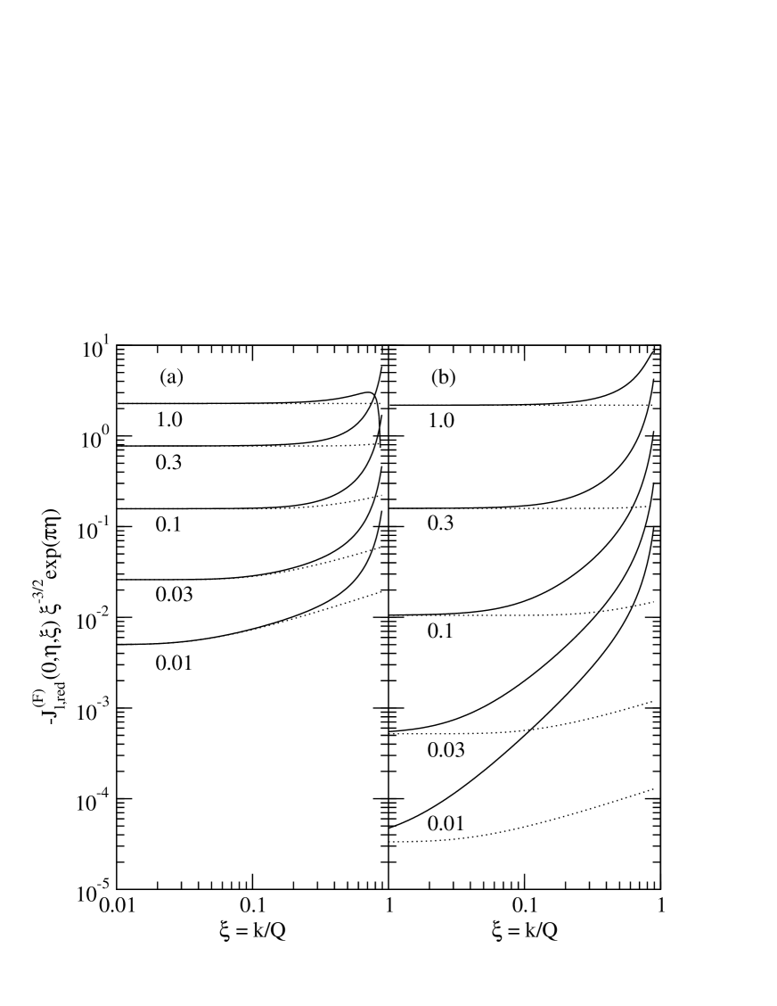
Figure 3: Scaled reduced Trojan-Horse integrals $-J_{l,{\rm red}}^{(F)}(0,\eta,\xi)\>\xi^{-\frac{3}{2}}\exp(\pi\eta)$ for parameters $\eta\xi=0.01,\dots,1.0$ as a function of $\xi=k/Q$ for angular momenta $l=0$ (a) and $l=1$ (b). The solid lines are the exact results and the dotted lines are the approximations of Sec. III.3.

Figure 3 shows the dependence of the scaled reduced TH integrals $J_{l,{\rm red}}^{(F)}(0,\eta,\xi)\>\xi^{-\frac{3}{2}}\exp(\eta\xi)$ with $l=0,1$ on $\xi=k/Q$ for various values of $\eta\xi=Z_{A}Z_{x}e^{2}\mu_{Ax}/(\hbar^{2}Q)$ which is a constant for given $Q$. The scaled TH integrals become constant for small $\xi$ as expected. The rapid decrease of the unscaled TH integrals with decreasing $\xi$ for constant $\eta\xi$ is obvious. The angular momentum barrier leads to a smaller TH integral with larger $l$ for the same parameters $\xi$ and $\eta\xi$. This effect is more pronounced for small $\eta\xi$ than for large $\eta\xi$ where the Coulomb barrier dominates the $\xi$ dependence. The approximations (75) and (76) agree very well with the exact results for the TH integrals with $l=0,1$ for large $\eta\xi$ and not too large $\xi$. The agreement is less satisfactory for small $\eta\xi$ and larger $l$ as one may expect, since then the angular momentum barrier is getting more important as compared to the Coulomb barrier.

The TH integrals with the irregular Coulomb wave functions reduce in the limit $k\to 0$ to the form

$$J_{0}^{(G)}(0,\eta,k,Q)=J_{0,{\rm red}}^{(G)}(0,\eta,\xi) \to \frac{\xi}{C_{0}(\eta)}\left[1-2\eta\xi\>f(2\eta\xi)\right]\>,$$ (78)

$$J_{1}^{(G)}(0,\eta,k,Q)=J_{1,{\rm red}}^{(G)}(0,\eta,\xi) \to \frac{\xi}{C_{0}(\eta)}\left[\frac{1}{\eta\xi}-f(2\eta\xi)-2\eta\xi\>g(2\eta\xi)\right]$$ (79)

with functions

$$f(x)=\int\limits_{0}^{\infty}dt\>\frac{e^{-xt}}{t^{2}+1} = \mbox{Ci}(x)\sin x-\left[\mbox{Si}(x)-\frac{\pi}{2}\right]\cos x\>,$$ (80)

$$g(x)=\int\limits_{0}^{\infty}dt\>\frac{te^{-xt}}{t^{2}+1} = -\mbox{Ci}(x)\cos x-\left[\mbox{Si}(x)-\frac{\pi}{2}\right]\sin x$$ (81)

that can be expressed in terms of the sine and cosine integrals $\mbox{Si}(x)$ and $\mbox{Ci}(x)$ Abr70 . The expressions inside the brackets in eqs. (78) and (79) are constants and the $k$-dependence of the TH integrals with the irregular Coulomb wave functions is determined by $\xi/C_{0}(\eta)$.

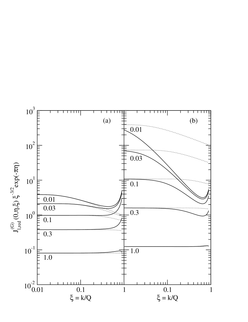
Figure 4: Scaled reduced Trojan-Horse integrals $J_{l,{\rm red}}^{(G)}(0,\eta,\xi)\>\xi^{-\frac{3}{2}}\exp(-\pi\eta)$ for parameters $\eta\xi=0.01,\dots,1.0$ as a function of $\xi=k/Q$ for angular momenta $l=0$ (a) and $l=1$ (b). The solid lines are the exact results and the dotted lines are the approximations of Sec. III.3.

In Figure 4 the dependence of scaled reduced TH integrals $J_{l,{\rm red}}^{(G)}(0,\eta,\xi)\>\xi^{-\frac{3}{2}}\exp(-\pi\eta)$ with $l=0,1$ on $\xi$ is shown for the same range of the parameter $\eta\xi$ as in Fig. 3. For small $\xi$ the scaled TH integrals again become constant. The unscaled TH integrals increase dramatically for decreasing $\xi$ for constant $\eta\xi$ and for increasing $\eta\xi$ for constant $\xi$, respectively. The effect of the angular momentum barrier is more pronounced for small $\eta\xi$ as in the case of the TH integrals with the regular Coulomb wave function as one may expect. The agreement between the approximations (78) and (79) and the exact TH integrals shows the same trends as in the case of the TH integrals with the regular Coulomb wave functions.

In the case of finite $R$ the energy dependence of the TH integrals for $\xi\to 0$ can be extracted with the help of the approximations (68) and (70) which are valid for $2\eta\gg\xi x_{0}$. The energy dependence of the differences

$$J_{l}^{(F)}(0,\eta,k,Q)-J_{l}^{(F)}(R,\eta,k,Q)=J_{l,{\rm red}}^{(F)}(0,\eta,\xi)-J_{l,{\rm red}}^{(F)}(x_{0},\eta,\xi)$$

$$\approx\frac{(2l+1)!C_{l}(\eta)\xi}{(2\eta)^{l+1}}\int\limits_{0}^{x_{0}}dx\>\sqrt{2\eta\xi x}\>I_{2l+1}(2\sqrt{2\eta\xi x})\>z_{l}(x)$$

and

$$J_{l}^{(G)}(0,\eta,k,Q)-J_{l}^{(G)}(R,\eta,k,Q)=J_{l,{\rm red}}^{(G)}(0,\eta,\xi)-J_{l,{\rm red}}^{(G)}(x_{0},\eta,\xi)$$

$$\approx\frac{2(2\eta)^{l}\xi}{(2l+1)!C_{l}(\eta)}\int\limits_{0}^{x_{0}}dx\>\sqrt{2\eta\xi x}\>K_{2l+1}(2\sqrt{2\eta\xi x})\>z_{l}(x)$$

is entirely given by the factor in front of the integrals since $\eta\xi=\eta k/Q$ is constant for constant $Q$. For large $\eta$ and small $\xi$ it is found that the energy dependence of the finite range correction to the TH integral with the regular and irregular Coulomb functions is given by $\xi^{2}C_{0}(\eta)$ and $\xi/C_{0}(\eta)$, respectively. The finite range correction essentially leads to a change in the absolute value of the integral but the energy dependence of $J_{l}^{(\pm)}(R,\eta,k,Q)$ and $J_{l}^{(\pm)}(0,\eta,k,Q)$ is the same for small $k$.

When the Sommerfeld parameter $\eta$ increases, the coefficient $C_{0}(\eta)$ becomes very small and the TH integral with $G_{l}$ is much larger than the TH integral with $F_{l}$. The integrals $J_{l}^{(\pm)}$ are therefore dominated by $J_{l}^{(G)}$ at low energies.

In the case where a neutron is transfered in reaction (3) the reduced TH integrals can be written as

$$J_{l}^{(\pm)}(R,0,k,Q)=J_{l,{\rm red}}^{(\pm)}(x_{0},0,\xi)=\frac{\pm i\xi^{2}x_{0}^{2}}{\xi^{2}-1}\left[\xi h_{l-1}^{(\pm)}(\xi x_{0})j_{l}(x_{0})-h_{l}^{(\pm)}(\xi x_{0})j_{l-1}(x_{0})\right]$$ (84)

in the variables $x_{0}=QR$ and $\xi=k/Q$ with $\eta=0$. For $\xi\to 0$ we find the approximation

$$J_{l,{\rm red}}^{(\pm)}(x_{0},0,\xi)\to\frac{(2l-1)!!}{(\xi x_{0})^{l-1}}\>j_{l-1}(x_{0})$$ (85)

with a distinct $l$-dependence due to the centrifugal barrier.

III.4 Simplified approximation of TH integrals

The dominance of the contribution with the irregular Coulomb wave function $G_{l}$ in the TH integrals $J_{l}^{(\pm)}$ at low energies also motivates a simple approximation in the limit $k\to 0$ that has been used in applications of the THM to reactions with $Ax\neq Cc$. In this case the integral is completely determined by the contributions at radii close to $R$ and the integrand decreases very fast with increasing $r$. If we assume that a general function $f(r)$ decreases exponentially, the integral of $f(r)$ from $R$ to infinity can be calculated from

$$\int\limits_{R}^{\infty}dr\>f(r)=f(R)\int\limits_{R}^{\infty}dr\>\exp\left(-\frac{r}{\Delta R}\right)=\Delta R\>f(R)$$ (86)

with $\Delta R=-f(R)/f^{\prime}(R)$ and $\mbox{Re}(\Delta R)>0$. In the TH integral $J_{l}^{(\pm)}$ the appropriate value of $\Delta R$ is determined by

$$\Delta R\approx-\left[\frac{kG_{l}^{\prime}(\eta;kR)}{G_{l}(\eta;kR)}+\frac{Qz_{l}^{\prime}(Qr)}{z_{l}(Qr)}\right]^{-1}$$ (87)

neglecting the small contribution of $F_{l}$ for $k\to 0$. From the approximation (70) of the irregular Coulomb wave function for $kR\ll 2\eta$ we find

$$\Delta R\approx-\left[\sqrt{\frac{2\eta k}{R}}\frac{K_{2l+1}^{\prime}(2\sqrt{2\eta kR})}{K_{2l+1}(2\sqrt{2\eta kR})}+\frac{Qz_{l}^{\prime}(Qr)}{z_{l}(Qr)}\right]^{-1}$$ (88)

independent of $k$ because $\eta k$ is constant and $Q$ is practically independent of $k$ for small $k$. Applying this result to the TH integral leads to the approximation

$$J_{l}^{(\pm)}(R,\eta,k,Q)=k\int\limits_{R}^{\infty}dr\>u_{l}^{(\pm)}(\eta;kr)\>z_{l}(Qr)\approx k\Delta R\>u_{l}^{(\pm)}(\eta;kR)\>z_{l}(QR)\>.$$ (89)

Since we are only interested in the $k$-dependence, the TH integral can be replaced by the value of the integrand

$$J_{l}^{(\pm)}(R,\eta,k,Q)\to k\>R\>u_{l}^{(\pm)}(\eta;kR)\>z_{l}(QR)$$ (90)

at the cutoff radius $R$ with the factor $R$ instead of $\Delta R$. The energy dependence for small $k$ in this simple approximation agrees with the exact result for the TH integrals.

IV Cross Sections for Spinless Particles

In order to establish a closer connection of the three-body and two-body cross sections the Trojan-Horse T-matrix element (49) is recast in the form

$$T_{fi}^{TH}(\vec{k}_{Cc},\vec{k}_{Bb};\vec{k}_{Aa})=\frac{4\pi}{k_{Ax}Q_{Aa}}\>W(\vec{Q}_{Bb})\>f^{TH}(\vec{Q}_{Aa},\vec{k}_{Cc})$$ (91)

with the Trojan-Horse scattering amplitude

$$f^{TH}(\vec{Q}_{Aa},\vec{k}_{Cc}) = \frac{k_{Ax}Q_{Aa}}{4\pi}\langle\Psi^{(-)}_{Cc,{\rm asym}}(\vec{k}_{Cc},\vec{r}_{Cc})|\exp\left(i\vec{Q}_{Aa}\cdot\vec{r}_{Ax}\right)\phi_{A}\phi_{x}\rangle$$

$$= \frac{1}{2ik_{Cc}}\sum_{l}(2l+1)P_{l}(\hat{k}_{Cc}\cdot\hat{Q}_{Aa})\sqrt{\frac{v_{Cc}}{v_{Ax}}}$$

$$\left[S^{l}_{AxCc}J_{l}^{(+)}(R,\eta_{Ax},k_{Ax},Q_{Aa})-\delta_{AxCc}J_{l}^{(-)}(R,\eta_{Ax},k_{Ax},Q_{Aa})\right]$$

which resembles an amplitude for the two-body reaction

$$C+c\to A+x\>.$$ (93)

The essential difference is the appearence of the Trojan-Horse integrals (47). The argument of the Legendre polynomial $P_{l}$ in equation (IV) corresponds to the usual cosine of the scattering angle $\vartheta_{cm}$. It is convenient to decompose the TH amplitude

$$f^{TH} = f_{N}^{TH}+f_{C}^{TH}\delta_{AxCc}$$ (94)

into a nuclear part and a purely Coulomb part. The nuclear contribution

$$f_{N}^{TH} = \frac{1}{2ik_{Cc}}\sum_{l}(2l+1)P_{l}(\hat{k}_{Cc}\cdot\hat{Q}_{Aa})\sqrt{\frac{v_{Cc}}{v_{Ax}}}T^{l}_{AxCc}J_{l}^{(+)}(R,\eta_{Ax},k_{Ax},Q_{Aa})$$ (95)

with

$$T^{l}_{AxCc}=e^{i\sigma_{l}(\eta_{Ax})+i\sigma_{l}(\eta_{Cc})}\left[S^{Nl}_{AxCc}-\delta_{AxCc}\right]$$ (96)

depends on the nuclear S-matrix element

$$S^{Nl}_{AxCc}=e^{-i\sigma_{l}(\eta_{Ax})}S^{l}_{AxCc}e^{-i\sigma_{l}(\eta_{Cc})}$$ (97)

which is obtained from the full S-matrix element by compensating the Coulomb phase shifts $\sigma_{l}(\eta_{Cc})$ and $\sigma_{l}(\eta_{Ax})$ in the initial and final states, respectively. The Coulomb contribution

$$f_{C}^{TH} = \frac{1}{k_{Cc}}\sum_{l}(2l+1)P_{l}(\hat{k}_{Cc}\cdot\hat{Q}_{Aa})e^{i\sigma_{l}(\eta_{Cc})}J_{l}^{(F)}(R,\eta_{Ax},k_{Ax},Q_{Aa})$$ (98)

appears only if elastic two-body reactions are studied. It depends only in the TH integrals with the regular Coulomb wave function and is discussed in Section VI.

If the Trojan-Horse integrals $J_{l}^{(\pm)}$ are replaced by one the scattering amplitudes reduce to the standard form for the reaction (93). At low energies there are usually only few contributions to the nuclear scattering amplitude with small angular momenta $l$ due to the increase of centrifugal barrier with $l$ in the two-body reaction.

The cross section (15) in the laboratory system can now be expressed in the form

$$\frac{d^{3}\sigma}{dE_{C}d\Omega_{C}d\Omega_{c}} = K_{\rm lab}\left|W(\vec{Q}_{Bb})\right|^{2}\frac{16\pi^{2}}{k_{Ax}^{2}Q_{Aa}^{2}}\frac{v_{Cc}}{v_{Ax}}\frac{d\sigma^{TH}}{d\Omega}$$ (99)

with the two-body Trojan-Horse cross section

$$\frac{d\sigma^{TH}}{d\Omega}=\frac{v_{Ax}}{v_{Cc}}\left|f^{TH}\right|^{2}\>.$$ (100)

A corresponding expression holds for the c.m. cross section (13) with the appropriate kinematical factor. This result has a similar structure as in the PWIA, i.e. a product of a kinematical factor, a momentum distribution and a two-body cross section. However, the momentum distribution $\left|W\right|^{2}$ is not directly the ground state momentum distribution $\left|\Phi_{a}\right|^{2}$ of the Trojan Horse $a$ and the Trojan-Horse cross section (100) contains explicitly the off-shell effects. It is a sum

$$\frac{d\sigma^{TH}}{d\Omega}=\left[\frac{d\sigma^{TH}_{C}}{d\Omega}+\frac{d\sigma^{TH}_{I}}{d\Omega}\right]\delta_{AxCc}+\frac{d\sigma^{TH}_{N}}{d\Omega}$$ (101)

of a Coulomb contribution

$$\frac{d\sigma^{TH}_{C}}{d\Omega}=\left|f^{TH}_{C}\right|^{2}$$ (102)

a Coulomb-nuclear interference contribution

$$\frac{d\sigma^{TH}_{I}}{d\Omega} = \sum_{l}\frac{2l+1}{k_{Cc}}P_{l}(\hat{k}_{Cc}\cdot\hat{Q}_{Aa})\>\mbox{Re}\left[\left(if^{TH}_{C}\right)^{\ast}T^{l}_{AxCc}J_{l}^{(+)}(R,\eta_{Ax},k_{Ax},Q_{Aa})\right]$$ (103)

and a nuclear contribution

$$\frac{d\sigma^{TH}_{N}}{d\Omega} = \frac{1}{4k_{Cc}^{2}}\sum_{\lambda}\sum_{ll^{\prime}}(2l+1)(2l^{\prime}+1)(l\>0\>l^{\prime}\>0|\lambda\>0)^{2}P_{\lambda}(\hat{k}_{Cc}\cdot\hat{Q}_{Aa})$$

$$T^{l}_{AxCc}T^{l^{\prime}\ast}_{AxCc}J_{l}^{(+)}(R,\eta_{Ax},k_{Ax},Q_{Aa})J_{l^{\prime}}^{(-)}(R,\eta_{Ax},k_{Ax},Q_{Aa})\>.$$

Again, the expression for the TH cross section closely resembles the usual c.m. cross section for the two-body reaction (93). The appearence of the TH integrals $J_{l}^{(\pm)}$ accounts for the off-shell effects and the scalar product $\hat{k}_{Cc}\cdot\hat{Q}_{Aa}$ appears as the argument of the Legendre polynomial instead of the cosine of the two-body c.m. scattering angle $\vartheta_{cm}$. The TH Coulomb scattering amplitude (98) replaces the on-shell Coulomb scattering amplitude

$$f_{C} = \frac{1}{2ik_{Cc}}\sum_{l}(2l+1)P_{l}(\cos\vartheta_{cm})\left(\exp[2i\sigma_{l}(\eta_{Cc})]-1\right)$$

$$= -\frac{\eta_{Cc}}{2k_{Cc}\sin^{2}\frac{\vartheta_{cm}}{2}}\exp\left[2i\sigma_{0}(\eta_{Cc})-2i\eta_{Cc}\ln\sin\frac{\vartheta_{cm}}{2}\right]$$

in the usual elastic two-body scattering amplitude.

The expression for the TH cross section simplifies considerably in special cases. If $Ax\neq Cc$ and only one partial wave $l_{Ax}$ contributes to the cross section the Trojan-Horse cross section is given by

$$\frac{d\sigma^{TH}}{d\Omega}=\frac{d\sigma_{l}}{d\Omega}(Cc\to Ax)\>P_{l}(R,\eta_{Ax},k_{Ax},Q_{Aa})$$ (106)

with the usual partial on-shell cross section

$$\frac{d\sigma_{l}}{d\Omega}(Cc\to Ax) = \frac{(2l+1)^{2}}{4k_{Cc}^{2}}\left|T^{l}_{AxCc}\right|^{2}\sum_{\lambda}(l\>0\>l\>0|\lambda\>0)^{2}P_{\lambda}(\hat{k}_{Cc}\cdot\hat{Q}_{Aa})$$ (107)

for the two-body reaction (93) and the penetrability factor

$$P_{l}(R,\eta_{Ax},k_{Ax},Q_{Aa})=\left|J_{l}^{(+)}(R,\eta_{Ax},k_{Ax},Q_{Aa})\right|^{2}\>.$$ (108)

In the simple approximation of Sec. III.4 it is given by

$$P_{l}(R,\eta,k,Q)\to k^{2}R^{2}\left[F_{l}^{2}(\eta;kR)+G_{l}^{2}(\eta;kR)\right]\>z_{l}^{2}(QR)\>.$$ (109)

From the $k$-dependence of the TH integrals or the Coulomb wave functions a $k^{3}\exp(2\pi\eta)$ behaviour of the penetrability factor is found for $k\to 0$. For the transfer of a neutron the dependence of $P_{l}$ on small $k$ is given by $k^{2-2l}$, see eq. (85), with an $l$-dependence determined by the centrifugal barrier.

With the theorem of detailed balance one obtains the direct relation

$$\frac{d^{3}\sigma}{dE_{C}d\Omega_{C}d\Omega_{c}} = K_{\rm lab}\left|W(\vec{Q}_{Bb})\right|^{2}\frac{16\pi^{2}}{k_{Cc}^{2}Q_{Aa}^{2}}\frac{v_{Cc}}{v_{Ax}}\frac{d\sigma_{l}}{d\Omega}(Ax\to Cc)\>P_{l}(R,\eta_{Ax},k_{Ax},Q_{Aa})$$ (110)

of the three-body cross section to the two-body cross section for partial wave $l$. This equation shows clearly the “parallelism” of the $A+x$ reaction and the Trojan-Horse reaction: The cross section (110) is proportional to the cross section for the $A+x$ reaction, modulated by the penetrability factor $P_{l}$. The factor $P_{l}$ is directly related to the TH integrals (108). It leads in general to an enhancement of the higher partial waves and it contains the $\exp(2\pi\eta)$ factor.

A most convincing beautiful example of this parallelism is the comparison of neutron elastic scattering and the $(d,p)$ reaction on ¹⁵N in the same energy range of the continuum in ¹⁶N. There are the same peaks in both spectra, changed in magnitude according to the factor $P_{l}$ ($\eta=0$ in the neutron transfer case). Also the s-wave resonance which appears as a destructive interference with the $l=0$ continuum shows up nicely in the $(d,p)$ spectrum Fuc71 .

V Cross Sections for Particles with Spin

For the application of the THM to a particular reaction one has to consider that the nuclei participating in the reactions (2) and (3) usually carry a spin. In this case the definition of the relevant quantities becomes more intricate but the general procedure remains the same as in the spinless case. Spins of an individual particle $i$ will be denoted in the following by $s_{i}$ with projection $\nu_{i}$.

Here, the channel spin basis in the derivation of the expressions is used. In the two-particle reaction the spins $s_{A}$ and $s_{x}$ in the initial state are coupled to the channel spin $s_{Ax}$. Similarly, in the final state $s_{C}$ and $s_{c}$ are coupled to the channel spin $s_{Cc}$. Coupling $s_{Cc}$ with the spin of the spectator $s_{b}$ gives the angular momentum $s_{f}$ of the three-body final state. The initial state of reaction (3) is characterized by the angular momentum $s_{i}$ which is obtained from coupling the spins $s_{A}$ and $s_{a}$.

The cross section of reaction (3) in the laboratory system

$$\frac{d^{3}\sigma}{dE_{C}d\Omega_{C}d\Omega_{c}} = \frac{K_{\rm lab}}{(2s_{A}+1)(2s_{a}+1)}\sum_{s_{i}s_{f}}\sum_{\nu_{i}\nu_{f}}\sum_{s_{Cc}}\left|T_{fi}(\vec{k}_{Cc},\vec{k}_{Bb},s_{Cc}s_{f}\nu_{f};\vec{k}_{Aa},s_{i}\nu_{i})\right|^{2}$$ (111)

is obtained by summing over final spin states and averaging over initial spin states with the three-body T-matrix element $T_{fi}$ that carries now both momentum and spin indices. In the plane wave approximation it is given by

$$T_{fi}^{TH}(\vec{k}_{Cc},\vec{q}_{Bb},s_{Cc}s_{f}\nu_{f};\vec{q}_{Aa},s_{i}\nu_{i})$$

$$= \langle\exp\left(i\vec{q}_{Bb}\cdot\vec{r}_{Bb}\right)\Psi^{(-)}_{\rm asym}(Cc-b,\vec{k}_{Cc},s_{f}\nu_{f})|V_{xb}|\exp\left(i\vec{q}_{Aa}\cdot\vec{r}_{Aa}\right)\phi_{Aa}(s_{i}\nu_{i})\rangle$$

with the asymptotic wave function

$$\Psi^{(-)}_{\rm asym}(Cc-b,\vec{k}_{Cc},s_{Cc},s_{f}\nu_{f})$$

$$= \sum_{\nu_{Cc}\nu_{b}}(s_{Cc}\>\nu_{Cc}\>s_{b}\>\nu_{b}|s_{f}\>\nu_{f})\Psi^{(-)}_{\rm asym}(Cc,\vec{k}_{Cc},s_{Cc}\nu_{Cc})\phi_{b}(s_{b}\nu_{b})$$

where

$$\Psi^{(\pm)}_{\rm asym}(Cc,\vec{k}_{Cc},s_{Cc},\nu_{Cc})$$

$$= \frac{4\pi}{k_{Cc}}\sum_{\alpha s_{\alpha}}\sum_{JM}\sum_{l_{\alpha}l_{Cc}}\frac{1}{r_{\alpha}}\xi^{J(\pm)}_{l_{\alpha}s_{\alpha}l_{Cc}s_{Cc}}(\alpha;k_{\alpha}r_{\alpha}){\cal Y}_{JM}^{l_{\alpha}s_{\alpha}}(\alpha,\hat{r}_{\alpha}){\cal Z}_{JM}^{l_{Cc}s_{Cc}\nu_{Cc}\ast}(\hat{k}_{Cc})$$

for $r_{\alpha}\geq R$ and $\Psi^{(\pm)}_{\rm asym}=0$ for $r_{\alpha}<R$. The vector spherical harmonics

$${\cal Y}_{JM}^{ls}(\alpha,\hat{r})=\sum_{m\nu}(l\>m\>s\>\nu|J\>M)i^{l}Y_{lm}(\hat{r})\phi_{\alpha}(s\nu)$$ (115)

and the angular distribution functions

$${\cal Z}_{JM}^{ls\nu}(\hat{k})=\sum_{m}(l\>m\>s\>\nu|J\>M)Y_{lm}(\hat{k})\>.$$ (116)

are obtained by coupling the channel spins $s$ with the corresponding orbital angular momenta $l$ to the total angular momentum $J$. The radial wave functions

$$\xi^{J(+)}_{l_{\alpha}s_{\alpha}l_{Cc}s_{Cc}}(\alpha;k_{\alpha}r_{\alpha})=\frac{1}{2i}\sqrt{\frac{v_{Cc}}{v_{\alpha}}}$$

$$\left[S^{J\alpha Cc}_{l_{\alpha}s_{\alpha}l_{Cc}s_{Cc}}u_{l_{\alpha}}^{(+)}(\eta_{\alpha};k_{\alpha}r_{\alpha})-\delta_{\alpha Cc}\delta_{l_{\alpha}l_{Cc}}\delta_{s_{\alpha}s_{Cc}}u_{l_{\alpha}}^{(-)}(\eta_{\alpha};k_{\alpha}r_{\alpha})\right]$$

and

$$\xi^{J(-)}_{l_{\alpha}s_{\alpha}l_{Cc}s_{Cc}}(\alpha;k_{\alpha}r_{\alpha})=\xi^{J(+)\ast}_{l_{\alpha}s_{\alpha}l_{Cc}s_{Cc}}(\alpha;k_{\alpha}r_{\alpha})$$ (118)

contain the general S-matrix elements $S^{J\alpha Cc}_{l_{\alpha}s_{\alpha}l_{Cc}s_{Cc}}$ for a transition from a channel with quantum numbers $l_{Cc}s_{CC}$ in the partition $Cc$ to the channel $l_{\alpha}s_{\alpha}$ in partition $\alpha$.

The T-matrix in the plane wave approximation

$$T_{fi}^{TH}(\vec{k}_{Cc},\vec{q}_{Bb},s_{Cc}s_{f}\nu_{f};\vec{q}_{Aa},s_{i}\nu_{i}) = \frac{4\pi}{k_{Ax}Q_{Aa}}\>W(\vec{Q}_{Bb})\>{\cal F}^{TH}(\vec{Q}_{Aa},\vec{k}_{Cc},s_{Cc}s_{f}\nu_{f}s_{i}\nu_{i})$$ (119)

again factorizes into a form with the momentum amplitude $W$ and the scattering amplitude

$${\cal F}^{TH}(\vec{Q}_{Aa},\vec{k}_{Cc},s_{Cc}s_{f}\nu_{f}s_{i}\nu_{i})=$$

$$\frac{1}{2ik_{Cc}}\sum_{J}\sum_{s_{Ax}}\sum_{l_{Ax}l_{Cc}}(2J+1){\cal P}_{l_{Ax}s_{Ax}l_{Cc}s_{Cc}}^{J}(\hat{k}_{Cc},\hat{Q}_{Aa},s_{f}\nu_{f}s_{i}\nu_{i})\sqrt{\frac{v_{Cc}}{v_{Ax}}}$$

$$\left[S^{JAxCc}_{l_{Ax}s_{Ax}l_{Cc}s_{Cc}}J_{l_{Ax}}^{(+)}(R,\eta_{Ax},k_{Ax},Q_{Aa})-\delta_{AxCc}\delta_{l_{Ax}l_{Cc}}\delta_{s_{Ax}s_{Cc}}J_{l_{Ax}}^{(-)}(R,\eta_{Ax},k_{Ax},Q_{Aa})\right]$$

which is a matrix in spin space. The angular distribution is determined by the function

$${\cal P}_{l_{Ax}s_{Ax}l_{Cc}s_{Cc}}^{J}(\hat{k}_{Cc},\hat{Q}_{Aa},s_{f}\nu_{f}s_{i}\nu_{i})$$

$$= \frac{4\pi}{2J+1}\sum_{\nu_{x}\nu_{b}}\sum_{\nu_{A}\nu_{a}}\sum_{m_{Cc}\nu_{Cc}}\sum_{m_{Ax}\nu_{Ax}}\sum_{M}Y_{l_{Cc}m_{Cc}}(\hat{k}_{Cc})Y_{l_{Ax}m_{Ax}}^{\ast}(\hat{Q}_{Aa})$$

$$(s_{x}\>\nu_{x}\>s_{b}\>\nu_{b}|s_{a}\>\nu_{a})(s_{A}\>\nu_{A}\>s_{a}\>\nu_{a}|s_{i}\>\nu_{i})(s_{Cc}\>\nu_{Cc}\>s_{b}\>\nu_{b}|s_{f}\>\nu_{f})$$

$$(l_{Ax}\>m_{Ax}\>s_{Ax}\>\nu_{Ax}|J\>M)(s_{A}\>\nu_{A}\>s_{x}\>\nu_{x}|s_{Ax}\>\nu_{Ax})(l_{Cc}\>m_{Cc}\>s_{Cc}\>\nu_{Cc}|J\>M)$$

$$= 4\pi\sum_{m_{Ax}m_{Cc}}\sum_{jm}(s_{i}\>\nu_{i}\>j\>m|s_{f}\>\nu_{f})(l_{Cc}\>m_{Cc}\>j\>m|l_{Ax}\>m_{Ax})$$

$$Y_{l_{Cc}m_{Cc}}(\hat{k}_{Cc})Y_{l_{Ax}m_{Ax}}^{\ast}(\hat{Q}_{Aa}){\cal X}_{l_{Ax}s_{Ax}l_{Cc}s_{Cc}}^{Jjs_{i}s_{f}}(s_{x},s_{b},s_{a},s_{A})$$

with

$${\cal X}_{l_{Ax}s_{Ax}l_{Cc}s_{Cc}}^{Jjs_{i}s_{f}}(s_{x},s_{b},s_{a},s_{A})$$ (129)

$$= (-1)^{s_{Ax}-s_{x}-s_{A}-j}\frac{(-1)^{s_{Ax}+J+l_{Cc}}}{\sqrt{2s_{Ax}+1}\sqrt{2l_{Ax}+1}}\sqrt{2s_{a}+1}\sqrt{2s_{i}+1}$$

$$(2j+1)(2s_{Ax}+1)\left\{\begin{array}[]{ccc}s_{x}&s_{A}&s_{Ax}\\ s_{i}&s_{b}&s_{a}\end{array}\right\}\left\{\begin{array}[]{ccc}s_{Ax}&s_{b}&s_{i}\\ s_{f}&j&s_{Cc}\end{array}\right\}\left\{\begin{array}[]{ccc}s_{Ax}&J&l_{Ax}\\ l_{Cc}&j&s_{Cc}\end{array}\right\}\>.$$

The Trojan-Horse scattering amplitude is a sum

$${\cal F}^{TH} = {\cal F}_{N}^{TH}+{\cal F}_{C}^{TH}\delta_{AxCc}$$ (130)

of the pure Coulomb contribution

$${\cal F}_{C}^{TH} = \frac{1}{k_{Cc}}\sum_{J}\sum_{s_{Ax}}\sum_{l_{Ax}l_{Cc}}(2J+1){\cal P}_{l_{Ax}s_{Ax}l_{Cc}s_{Cc}}^{J}(\hat{k}_{Cc},\hat{Q}_{Aa},s_{f}\nu_{f}s_{i}\nu_{i})$$

$$e^{i\sigma_{l_{Ax}}(\eta_{Cc})}J_{l_{Ax}}^{(F)}(R,\eta_{Ax},k_{Ax},Q_{Aa})\delta_{l_{Ax}l_{Cc}}\delta_{s_{Ax}s_{Cc}}$$

$$= f^{TH}_{C}\delta_{\nu_{i}\nu_{f}}\delta_{s_{i}s_{f}}(-1)^{s_{x}+s_{A}+s_{b}+s_{f}}\sqrt{2s_{Cc}+1}\sqrt{2s_{a}+1}\left\{\begin{array}[]{ccc}s_{x}&s_{A}&s_{Cc}\\ s_{f}&s_{b}&s_{a}\end{array}\right\}$$ (134)

and the nuclear contribution

$${\cal F}_{N}^{TH} = \frac{1}{2ik_{Cc}}\sum_{J}\sum_{s_{Ax}}\sum_{l_{Ax}l_{Cc}}(2J+1){\cal P}_{l_{Ax}s_{Ax}l_{Cc}s_{Cc}}^{J}(\hat{k}_{Cc},\hat{Q}_{Aa},s_{f}\nu_{f}s_{i}\nu_{i})$$

$$\sqrt{\frac{v_{Cc}}{v_{Ax}}}T^{JAxCc}_{l_{Ax}s_{Ax}l_{Cc}s_{Cc}}J_{l_{Ax}}^{(+)}(R,\eta_{Ax},k_{Ax},Q_{Aa})$$

with

$$T^{JAxCc}_{l_{Ax}s_{Ax}l_{Cc}s_{Cc}} = e^{i\sigma_{l_{Ax}}(\eta_{Ax})+i\sigma_{l_{Cc}}(\eta_{Cc})}\left[S^{JAxCcN}_{l_{Ax}s_{Ax}l_{Cc}s_{Cc}}-\delta_{AxCc}\delta_{l_{Ax}l_{Cc}}\delta_{s_{Ax}s_{Cc}}\right]$$ (136)

depending on the nuclear S-matrix element $S^{JAxCcN}_{l_{Ax}s_{Ax}l_{Cc}s_{Cc}}$.

The unpolarized cross section for the three-body reaction in the laboratory system

$$\frac{d^{3}\sigma}{dE_{C}d\Omega_{C}d\Omega_{c}} = \frac{K_{\rm lab}}{(2s_{A}+1)(2s_{a}+1)}\sum_{\nu_{i}\nu_{f}}\sum_{s_{i}s_{f}}\sum_{s_{Cc}}\left|T_{fi}(\vec{k}_{Cc},\vec{k}_{Bb},s_{Cc}s_{f}\nu_{f};\vec{k}_{Aa},s_{i}\nu_{i})\right|^{2}$$

$$= K_{\rm lab}\left|W(\vec{Q}_{Bb})\right|^{2}\frac{16\pi^{2}}{k_{Ax}^{2}Q_{Aa}^{2}}\frac{v_{Cc}}{v_{Ax}}\frac{d\sigma^{TH}}{d\Omega}$$

is obtained by a summation over the spins in the final state and an averaging over the spins in the initial state. As in the case of spinless particles, the TH cross section

$$\frac{d\sigma^{TH}}{d\Omega} = \frac{1}{(2s_{A}+1)(2s_{a}+1)}\sum_{s_{i}s_{f}}\sum_{\nu_{i}\nu_{f}}\sum_{s_{Cc}}\frac{v_{Ax}}{v_{Cc}}\left|{\cal F}^{TH}\right|^{2}$$

$$= \left[\frac{d\sigma^{TH}_{C}}{d\Omega}+\frac{d\sigma^{TH}_{I}}{d\Omega}\right]\delta_{AxCc}+\frac{d\sigma^{TH}_{N}}{d\Omega}$$

decomposes into a pure Coulomb contribution

$$\frac{d\sigma^{TH}_{C}}{d\Omega} = \frac{1}{(2s_{A}+1)(2s_{a}+1)}\sum_{s_{i}s_{f}}\sum_{\nu_{i}\nu_{f}}\sum_{s_{Cc}}\left|{\cal F}^{TH}_{C}\right|^{2}=\left|f^{TH}_{C}\right|^{2}$$ (139)

an interference contribution

$$\frac{d\sigma^{TH}_{I}}{d\Omega} = \frac{1}{(2s_{A}+1)(2s_{a}+1)}\sum_{s_{i}s_{f}}\sum_{\nu_{i}\nu_{f}}\sum_{s_{Cc}}2\mbox{Re}\left[{\cal F}^{TH\ast}_{C}{\cal F}^{TH}_{N}\right]$$

$$= \frac{1}{(2s_{A}+1)(2s_{x}+1)}\sum_{J}\sum_{l_{Cc}}\sum_{s_{Cc}}\frac{2J+1}{k_{Cc}}$$

$$\mbox{Re}\left[\left(if^{TH}_{C}\right)^{\ast}T^{JCcCc}_{l_{Cc}s_{Cc}l_{Cc}s_{Cc}}J_{l_{Cc}}^{(+)}(R,\eta_{Ax},k_{Ax},Q_{Aa})\right]P_{l_{Cc}}(\hat{k}_{Cc}\cdot\hat{Q}_{Aa})$$

and a nuclear contribution

$$\frac{d\sigma^{TH}_{N}}{d\Omega} = \frac{1}{(2s_{A}+1)(2s_{a}+1)}\sum_{s_{i}s_{f}}\sum_{\nu_{i}\nu_{f}}\sum_{s_{Cc}}\frac{v_{Ax}}{v_{Cc}}\left|{\cal F}^{TH}_{N}\right|^{2}$$

$$= \frac{1}{(2s_{A}+1)(2s_{x}+1)}\frac{1}{4k_{Cc}^{2}}\sum_{\lambda}\sum_{JJ^{\prime}}\sum_{s_{Ax}s_{Cc}}\sum_{l_{Ax}l_{Cc}}\sum_{l_{Ax}^{\prime}l_{Cc}^{\prime}}$$

$$(-1)^{s_{Ax}-s_{Cc}}Z_{l_{Ax}l_{Ax}^{\prime}}^{JJ^{\prime}}(\lambda s_{Ax})Z_{l_{Cc}l_{Cc}^{\prime}}^{JJ^{\prime}}(\lambda s_{Cc})P_{\lambda}(\hat{Q}_{Aa}\cdot\hat{k}_{Cc})$$

$$T^{JAxCc}_{l_{Ax}s_{Ax}l_{Cc}s_{Cc}}T^{J^{\prime}AxCc\ast}_{l_{Ax}^{\prime}s_{Ax}l_{Cc}^{\prime}s_{Cc}}J_{l_{Ax}}^{(+)}(R,\eta_{Ax},k_{Ax},Q_{Aa})J_{l_{Ax}^{\prime}}^{(-)}(R,\eta_{Ax},k_{Ax},Q_{Aa})$$

with factors

$$Z_{ll^{\prime}}^{JJ^{\prime}}(\lambda s) = \sqrt{(2J+1)(2J^{\prime}+1)(2l+1)(2l^{\prime}+1)}\>(l\>0\>l^{\prime}\>0|\lambda\>0)\left\{\begin{array}[]{ccc}l&\lambda&l^{\prime}\\ J^{\prime}&s&J\end{array}\right\}$$ (144)

for the angular momentum coupling. The Coulomb contribution is the same as in the case of spinless particles. Notice the change from $s_{a}$ to $s_{x}$ in the spin degeneracy factors.

If only one orbital angular momentum $l=l_{Ax}=l_{Ax}^{\prime}$ contributes in the $Ax$ partition to the inelastic two-body reaction $A+x\to C+c$, the TH cross section

$$\frac{d\sigma^{TH}}{d\Omega}=\frac{(2s_{C}+1)(2s_{c}+1)}{(2s_{A}+1)(2s_{x}+1)}\frac{d\sigma_{l}}{d\Omega}(Cc\to Ax)\>P_{l}(R,\eta_{Ax},k_{Ax},Q_{Aa})$$ (145)

is directly related to the usual on-shell cross section

$$\frac{d\sigma_{l}}{d\Omega}(Cc\to Ax) = \frac{1}{(2s_{C}+1)(2s_{c}+1)}\frac{1}{4k_{Cc}^{2}}\sum_{\lambda}\sum_{JJ^{\prime}}\sum_{s_{Ax}s_{Cc}}\sum_{l_{Cc}l_{Cc}^{\prime}}$$

$$(-1)^{s_{Ax}-s_{Cc}}Z_{ll}^{JJ^{\prime}}(\lambda s_{Ax})Z_{l_{Cc}l_{Cc}^{\prime}}^{JJ^{\prime}}(\lambda s_{Cc})P_{\lambda}(\hat{Q}_{Aa}\cdot\hat{k}_{Cc})$$

$$T^{JAxCc}_{ls_{Ax}l_{Cc}s_{Cc}}T^{J^{\prime}AxCc\ast}_{ls_{Ax}l_{Cc}^{\prime}s_{Cc}}$$

with the penetrability factor (108). In (145) the only difference to the case with spinless particles is the appearance of the spin degeneracy factors. Applying the theorem of detailed balance the simple relation

$$\frac{d^{3}\sigma}{dE_{C}d\Omega_{C}d\Omega_{c}} = K_{\rm lab}\left|W(\vec{Q}_{Bb})\right|^{2}\frac{16\pi^{2}}{k_{Cc}^{2}Q_{Aa}^{2}}\frac{v_{Cc}}{v_{Ax}}\frac{d\sigma_{l}}{d\Omega}(Ax\to Cc)\>P_{l}(R,\eta_{Ax},k_{Ax},Q_{Aa})$$ (147)

is found which is the same as in the spinless case. The increase of the factor $P_{l}$ at small $k_{Ax}$ compensates the decrease of the two-body cross section $\frac{d\sigma_{l}}{d\Omega}(Ax\to Cc)$.

VI Trojan-Horse Coulomb Scattering Amplitude

In case of an inelastic two-body reaction only the nuclear contribution to the TH scattering amplitude is relevant. For the elastic scattering with $Ax=Cc$ also the TH Coulomb scattering amplitude (98) contributes to the total TH scattering amplitude. It depends only on the TH integrals $J_{l}^{(F)}$ with the regular Coulomb wave functions. The summation over $l$ in eq. (98) poses no serious problem but it is convenient to reformulate the expression as in the case of the TH integrals in order to see the reduction of the Coulomb barrier more clearly. For that purpose the TH Coulomb scattering amplitude is written as a difference

$$f_{C}^{TH}=f_{C0}^{TH}-f_{CR}^{TH}$$ (148)

of a contribution (suppressing the indices of the momenta)

$$f_{C0}^{TH} = \frac{2\eta k^{2}Q}{k^{2}-Q^{2}}\sum_{l}(2l+1)P_{l}(\hat{k}\cdot\hat{Q})e^{i\sigma_{l}(\eta)}M_{ll}^{-1}(F_{l},\eta,k,Q)$$ (149)

where the cutoff radius $R$ is set to zero and a finite range contribution

$$f_{CR}^{TH} = \sum_{l}(2l+1)P_{l}(\hat{k}\cdot\hat{Q})e^{i\sigma_{l}(\eta)}L_{l}(R,\eta,k,Q)$$ (150)

with the integrals

$$L_{l}(R,\eta,k,Q)=\int\limits_{0}^{R}dr\>F_{l}(\eta;kr)\>z_{l}(Qr)\>.$$ (151)

These are easily calculated numerically and decrease rapidly with increasing $l$ leading to a rapid convergence of the sum (150). Similar to relation (IV) for the full TH scattering amplitude, the contribution (149) to the TH Coulomb scattering amplitude can be expressed as a matrix element

$$f_{C0}^{TH} = \frac{kQ}{4\pi}\langle\Psi^{(-)}_{\rm Coul}(\vec{k})|\exp\left(i\vec{Q}\cdot\vec{r}\right)\rangle$$ (152)

with the pure Coulomb scattering wave function

$$\Psi^{(\pm)}_{\rm Coul}(\vec{k})=e^{-\frac{\pi}{2}\eta}\Gamma(1\pm i\eta)\exp(i\vec{k}\cdot\vec{r}){}_{1}F_{1}(\mp i\eta,1;\pm i[kr\mp\vec{k}\cdot\vec{r}])$$ (153)

where ${}_{1}F_{1}$ denotes a confluent hypergeometric function. This form allows an analytical calculation with the result

$$f_{C0}^{TH} = -\frac{2\eta k^{2}Q}{Q^{2}-k^{2}}\frac{C_{0}(\eta)}{(\vec{Q}-\vec{k})^{2}}\exp\left\{i\sigma_{0}(\eta)+i\eta\ln\left[\frac{Q^{2}-k^{2}}{(\vec{Q}-\vec{k})^{2}}\right]\right\}$$ (154)

as explained in Appendix B. Contrary to the ususal Coulomb scattering amplitude (IV) there is no divergence for $k\to 0$ since $Q$ remains finite. In this limit, the energy dependence of the TH Coulomb scattering amplitude is given by $kC_{0}(\eta)$. The apperance of the $C_{0}(\eta)$ factor in the amplitude causes a strong reduction at small $k$.

VII Applications of the Trojan-Horse Method

Several reactions have been studied with the TH method recently. They are listed in Table 1 with ²H and ⁶Li ($=\alpha+$d) as typical “Trojan Horses”. These nuclei allow to study the transfer of protons, neutrons, deuterons and $\alpha$-particles, which covers most of the cases of astrophysical interest for the two-body reaction.

Table 1: Projectile energy $E_{\rm pro}$ and corresponding quasi-free energy $E_{Ax}^{qf}$ for pairs of two-body and Trojan-Horse reactions.

two-body	Trojan-Horse	$E_{\rm pro}$	$E_{Ax}^{qf}$	Ref.
reaction	reaction	[MeV]	[MeV]
2H(6Li,4He)4He	6Li(6Li,4He4He)4He	6.0	0.029	Mus01 ; Spi01 ; Che96
7Li(p,4He)4He	2H(7Li,4He4He)n	19.0 - 21.0	0.161 - 0.412	Lat01 ; Ali00 ; Spi99 ; Cal97
12C(4He,4He)12C	6Li(12C,4He12C)2H	12.0 - 18.0	1.527 - 3.027	Spi00 ; Pel00
3He(2H,p)4He	6Li(3He,p4He)4He	5.8	0.845	Mus02
6Li(p,3He)4He	2H(6Li,3He4He)n	25.0	1.362	Tum02

VII.1 Kinematical Conditions

The Trojan Horses employed so far have a dominant s-wave configuration in their gound state. Their momentum distribution $W(\vec{Q}_{Bb})$ has a maximum around zero. Correspondingly, the equation

$$\vec{Q}_{Bb}=0$$ (155)

defines the so-called quasi-free condition. In this region of the three-body phase space the cross section for the quasi-free reaction will reach a maximum. From this condition the corresponding quasi-free c.m. energy

$$E_{Ax}^{qf}=E_{Aa}\left(1-\frac{\mu_{Aa}}{\mu_{Bb}}\frac{\mu_{bx}^{2}}{m_{x}^{2}}\right)-\varepsilon_{a}$$ (156)

in the initial channel of the two-body reaction (2) is derived from energy conservation (11) assuming the plane wave approximation. It is obvious that even with a large c.m. energy $E_{Aa}$ in the entrance channel of the three-body reaction (3) a small energy $E_{Ax}$ can be reached if a suitable Trojan Horse $a$ is chosen. This is confirmed in Table 1 where the projectile energy in the laboratory system and the quasi-free energy are shown for several reactions.

The relation between $E_{Ax}^{qf}$ and $E_{Aa}$ is purely a kinematical consequence. It is not related to the Fermi motion of particle $x$ inside the Trojan Horse $a$ which would involve a dependence on the width of the momentum amplitude. However, in an actual experiment a cutoff in the momentum transfer $\vec{Q}_{Bb}$ is chosen to select the region where the quasi-free process dominates the cross section. This procedure limits the range in energies $E_{Ax}$ that are within reach in the experiment for a chosen projectile energy $E_{\rm pro}$.

In case of the quasi-free condition, all nuclei in the final state of reaction (3) are emitted in the same plane. The momentum of the spectator $b$ is in beam direction which makes it difficult to detect $b$ in the experiment. In the laboratory system the nuclei $C$ and $c$ are emitted under angles $\vartheta_{C}$ and $\vartheta_{c}$ on opposite sides of the beam axis. If the scattering angle $\vartheta_{cm}$ in the c.m. system of the two-body reaction is given, the angles $\vartheta_{C}$, $\vartheta_{c}$, the so-called quasi-free angles, are completely specified for a fixed beam energy from kinematical considerations.

As a consequence, the quasi-free condition determines the setup of the experiment. If a particular two-body reaction (2) is to be studied close to a c.m. energy $E_{Ax}$ and if the Trojan Horse $a$ is selected, then from equation (156) the appropriate beam energy can be extracted. Since the momentum amplitude $W$ has a finite width it is possible to study the two-body reaction in a certain energy window around $E_{Ax}$. The c.m. scattering angle $\vartheta_{cm}$ determines the arrangement of the detectors close the pair of quasi-free angles.

When $E_{Bb}$ is zero in (11) the maximum energy

$$E_{Ax}^{\rm max}=E_{Aa}-\varepsilon_{a}$$ (157)

in the two-body system is reached for a fixed c.m. energy $E_{Aa}$ in the entrance channel of the three-body reaction. In this case $\vec{k}_{Bb}=0$ and $\vec{Q}_{Aa}=\vec{k}_{Aa}$. The momenta of all nuclei $C$, $c$, and $b$ in the final state are parallel to the beam momentum in the laboratory system. Since $\varepsilon_{a}>0$ it follows that the relation

$$k_{Ax}<\sqrt{\frac{\mu_{Ax}}{\mu_{Aa}}}Q_{Aa}<Q_{Aa}$$ (158)

holds in all kinematically allowed regions of the phase space.

VII.2 Threshold behaviour of cross sections

The energy dependence of the two-body cross section

$$\frac{d\sigma}{d\Omega}(Ax\to Cc)=$$

$$\frac{1}{4k_{Ax}^{2}}\sum_{\lambda}\sum_{ll^{\prime}}(2l+1)(2l^{\prime}+1)(l\>0\>l^{\prime}\>0|\lambda\>0)^{2}P_{\lambda}(\cos\vartheta)S^{l}_{AxCc}S^{l^{\prime}\ast}_{AxCc}$$

for the inelastic $A+x\to C+c$ reaction above the reaction threshold is governed by the $1/k_{Ax}^{2}$ factor and energy dependence

$$S^{l}_{AxCc}\propto\exp(-\pi\eta_{Ax})$$ (160)

of the relevant S-matrix element. The Coulomb barrier leads to a strong suppression of the the cross section

$$\frac{d\sigma}{d\Omega}(Ax\to Cc)\propto k_{Ax}^{-2}\exp(-2\pi\eta_{Ax})$$ (161)

for $k_{Ax}\to 0$ due to the decreasing exponential factor. This behaviour motivates the introduction of the astrophysical S-factor (1). In the TH cross section $\frac{d\sigma^{TH}}{d\Omega}$, that appears in eq. (99), the factor $k_{Ax}^{-2}$ is replaced with $k_{Cc}^{-2}$ and the TH integrals $J_{l}^{(+)}$ appear. Their energy dependence for small $k_{Ax}$ is determined by $k_{Ax}/C_{0}(\eta_{Ax})\approx k_{Ax}\exp(\pi\eta_{Ax})/\sqrt{2\pi\eta_{Ax}}$ from the contribution of the irregular Coulomb wave function. This leads to a $k_{Ax}$ dependence of the three-body cross section (99) according to

$$\frac{d^{3}\sigma}{dE_{C}d\Omega_{C}d\Omega_{c}}\propto k_{Ax}^{-2}v_{Ax}^{-1}\exp(-2\pi\eta_{Ax})k_{Ax}^{2}\frac{\exp(2\pi\eta_{Ax})}{2\pi\eta_{Ax}}=\left(2\pi\eta_{Ax}v_{Ax}\right)^{-1}=\mbox{const.}$$ (162)

in the lowest order of $k_{Ax}$; cf. also eq. (110) with the $k_{Ax}$ dependence of the penetrability factor $P_{l}\propto k_{Ax}^{3}\exp(2\pi\eta_{Ax})$. As a result the cross section does not vanish at the treshold but takes on a finite value. Of course, the same considerations apply to the case when the spins of the particles are considered. Also in the case of the transfer of neutron, like in a (d,p) stripping reaction, it is well known that the cross section is finite at the threshold $E_{n}=0$ Bau84 ; Bau76 . The reason is the same as in the case of charged particles.

VII.3 Extraction of astrophysical S-factors

In an actual TH experiment the measured cross section of the three-body reaction depends on the geometry of the setup, the chosen Trojan Horse, and the energy of the projectile. The differential three-body cross section (99) or (110) can be projected onto a simple cross section

$$\frac{d\sigma}{dE}=\int dE_{C}d\Omega_{C}d\Omega_{c}\frac{d^{3}\sigma}{dE_{C}d\Omega_{C}d\Omega_{c}}\delta(E_{Ax}-E)F(E_{C},\Omega_{C},\Omega_{c})$$ (163)

depending on the $A+x$ c.m. energy $E$. The efficiency function $F$ takes cut-offs in particle energies, momenta (e.g. $\vec{Q}_{Bb}$), the detector geometry etc. into account. The experimental spectrum (163) can be compared to a corresponding theoretical cross section from a simulation of the experiment assuming a certain energy dependence of the relevant on-shell S-matrix elements of the two-body reaction, e.g. from a R-matrix parametrization. By a variation of the parameters, the best fit to the experiment is found and the on-shell two-body cross section can be calculated. If there is only a contribution of one partial wave, the procedure becomes simpler. The ratio of the measured cross section (163) to the corresponding simulated cross section directly gives the energy dependence of the S-factor relative to the energy dependence assumed in the theoretical S-factor of the two-body reaction. Due to the uncertainties in the description of the reaction mechanism it is expected to be difficult to extract absolute values of the cross section. So it is better to normalize the cross section to results from direct experiments at higher energies. However, we expect that the energy dependence of the cross section (S-factor) can be extracted much more reliably. For recent applications of the TH method with detailed information on the experimental realisation we refer to the references Mus01 ; Spi01 ; Che96 ; Lat01 ; Ali00 ; Spi99 ; Cal97 .

VII.4 Elastic scattering with the Trojan-Horse method

The main aim for applying the TH method is the extraction of the energy dependence of cross sections or astrophysical S-factors for inelastic two-body reactions. But also the indirect investigation of elasting two-body scattering $A+x\to A+x$ can be rewarding. In the direct two-body scattering process the cross section is dominated by the contribution of the Coulomb scattering amplitude (IV) at low energies that diverges with $k_{Ax}^{-2}$. By way of contrast, the TH Coulomb scattering amplitude (98) vanishes for $k_{Ax}\to 0$ due to the appearance of the TH integrals with the regular Coulomb wave function $F_{l}$. The nuclear contribution to the TH cross section (101) becomes dominant because of the TH integrals with the irregular Coulomb wave functions in eq. (IV). This allows the study of nuclear effects in the scattering at small energies, e.g. the influence of sub-threshold or low energy resonances. First attempt in this direction were made in recent experiments Spi00 ; Pel00 .

VIII Summary and Outlook

In this paper the basic theory of the Trojan-Horse method was developed starting from a distorted wave Born approximation of the T-matrix element. The essential surface approximation allows to find the relation between the cross section of the three-body reaction and the S-matrix elements of the astrophysically relevant two-body reaction. In the modified plane wave approximation the relation between the three-body and two-body cross sections becomes very transparent. The three-body cross section is a product of a kinematical factor, a momentum distribution and an off-shell two-body cross section. Off-shell effects are expressed in terms of so-called TH integrals that were studied in detail. Their energy dependence leads to a finite cross section of the three-body reaction at the threshold of the two-body reaction without the suppression by the Coulomb barrier. This allows to extract the energy dependence of astrophysical cross sections from the three-body breakup reaction to very low energies without the problems of electron screening and extremely low cross section. A comparison of results for S-factors from direct and indirect experiments can improve the information on the electron screening effect. However, dedicated Trojan-Horse experiments are necessary in order to achieve a precision comparable to direct measurements.

The validity of the Trojan-Horse method can be tested by comparing the cross sections extracted from the indirect experiment with results from direct measurements of well studied reactions. In principle it is possible to assess systematic uncertainties of the Trojan-Horse method by studying various combinations of projectile energies, spectators in the Trojan Horse and scattering angles. Furthermore, different theoretical approximations can be compared, e.g. full DWBA calculations with and without the surface approximation and simpler modified plane wave approximations.

One may also envisage applications of the Trojan-Horse method to exotic nuclear beams. An unstable projectile hits a Trojan Horse target allowing to study specific reactions on exotic nuclei. A study of low-energy elastic scattering with the Trojan-Horse method opens another application which can lead to improved information relevant to the theoretical description of nuclear reactions at low energies.

Appendix A Analytical Calculation of Radial Integrals

The radial integrals

$$M_{ll}^{-1}(H,\eta,k,Q)=\frac{1}{kQ}\int\limits_{0}^{\infty}dr\>H_{l}(\eta;kr)r^{-1}z_{l}(Qr)$$ (164)

appearing in equation (59) can be calculated explicitly by using the integral representation

$$F_{l}(\eta;kr)+iG_{l}(\eta;kr) = \frac{i(kr)^{l+1}}{(2l+1)!C_{l}(\eta)}\int\limits_{i}^{i+\infty}ds\>e^{-krs}(s-i)^{l-i\eta}(s+i)^{l+i\eta}$$ (165)

of the combined Coulomb function $H_{l}=F_{l}+iG_{l}$. This form has been obtained from the representation in Abr70 by the substitution $t=kr(s-i)$. The integration path in the variable $s$ is a parallel to the real axis in the complex plane. Since the recursion relation (67) connects integrals of three successive $l$-values, only the basic integrals with $l=0$ and $l=1$ are needed for the explicit calculation of $M_{ll}^{-1}$ for all $l$. With $z_{0}(x)=\sin x$ and $z_{1}(x)=\sin x/x-\cos x$ the integration over the radial coordinate $r$ is easily performed and one finds

$$M_{00}^{-1}(H,\eta,k,Q) = \frac{i}{C_{0}(\eta)}\int\limits_{i}^{i+\infty}ds\>\frac{(s+i)^{i\eta}(s-i)^{-i\eta}}{k^{2}s^{2}+Q^{2}}$$ (166)

and

$$M_{11}^{-1}(H,\eta,k,Q) = \frac{ikQ}{3C_{1}(\eta)}\int\limits_{i}^{i+\infty}ds\>\frac{(s+i)^{1+i\eta}(s-i)^{1-i\eta}}{(k^{2}s^{2}+Q^{2})^{2}}\>.$$ (167)

The substitution $s=i(t+1)/(t-1)$ leads to the expressions

$$M_{00}^{-1}(H,\eta,k,Q) = \frac{-2}{C_{0}(\eta)(Q^{2}-k^{2})}I_{0}(\eta,z)\>,$$ (168)

$$M_{11}^{-1}(H,\eta,k,Q) = \frac{4kQ}{3C_{1}(\eta)(Q^{2}-k^{2})^{2}}\frac{d}{dz}I_{0}(\eta,z)$$ (169)

with the integral

$$I_{0}(\eta,z)=\int\limits_{C}dt\>\frac{t^{i\eta}}{t^{2}-2tz+1}\>.$$ (170)

The contour $C$ is the straight line from $1$ to $1+i\infty$ parallel to the imaginary axis in the complex plane. The integral depends on the variable

$$z=\frac{Q^{2}+k^{2}}{Q^{2}-k^{2}}$$ (171)

which is always larger than 1 for the conditions of the TH method. The integrand has two poles at $z_{1}=z+\sqrt{z^{2}-1}>1$ and $z_{2}=z-\sqrt{z^{2}-1}<1$ on the real axis. In the next step the path of integration is deformed to lie on the real axis and the integrand is broken into partial fractions. This yields

$$I_{0}(\eta,z) = \int\limits_{1}^{\infty}dt\>\frac{t^{i\eta}}{t^{2}-2tz+1}-\pi i\>\mbox{Res}_{z_{1}}\frac{t^{i\eta}}{t^{2}-2tz+1}$$

$$= \frac{1}{z_{1}-z_{2}}\left[I_{1}-I_{2}-\pi iz_{1}^{i\eta}\right]$$

with the contribution of the residue at the pole $z_{1}$. The remaining integrals

$$I_{i} = \int\limits_{1}^{\infty}dt\>t^{i\eta}\left[\frac{1}{t-z_{i}}-\frac{1}{t}\right]$$ (173)

for $i=1,2$ are evaluated with the help of the geometric series and the relation Abr70

$$\frac{\pi\eta}{\tanh(\pi\eta)}=1+2\eta^{2}\sum_{n=1}^{\infty}\frac{1}{n^{2}+\eta^{2}}\>.$$ (174)

Collecting all contributions we find

$$I_{0}(\eta,z) = \frac{i}{2\eta\sqrt{z^{2}-1}}\left[C_{0}^{2}(\eta)\left(z_{1}^{i\eta}-1\right)-2\eta^{2}\sum_{n=1}^{\infty}\frac{z_{1}^{-n}-1}{n^{2}+\eta^{2}}-\pi\eta\right]$$ (175)

for the fundamental integral (170). Separating real and imaginary parts, the explicit expressions of the integrals $M_{00}^{-1}(H_{0},\eta,k,Q)$ and $M_{00}^{-1}(G_{0},\eta,k,Q)$ are found with eq. (168). In the case $l=1$ the derivative of $I_{0}(z)$ with respect to $z$ has to be calculated first.

Appendix B Trojan-Horse Coulomb Scattering Amplitude

Recalling the procedure to derive the radial integrals (164), the contribution $f_{C0}^{TH}$ to the Coulomb scattering amplitude can be written as

$$f_{C0}^{TH} = \frac{\eta k^{2}Q}{2\pi(k^{2}-Q^{2})}\langle\Psi^{(-)}_{\rm Coul}(\vec{k})|r^{-1}|\exp\left(i\vec{Q}\cdot\vec{r}\right)\rangle\>.$$ (176)

by considering the Schrödinger equations for the Coulomb scattering wave $\Psi^{(\pm)}_{\rm Coul}$ and the plane wave. The matrix element can be evaluated by employing the integral representation of the confluent hypergeometric function Abr70 in the Coulomb scattering wave function (153). After the integration over the spatial coordinates, an integral remains that represents a hypergeometric function Abr70 . This technique is similar to the evaluation of Bremsstrahlung matrix elements Nor54 ; Shy92 . One obtains

$$\langle\Psi^{(-)}_{\rm Coul}(\vec{k})|r^{-1}|\exp\left(i\vec{Q}\cdot\vec{r}\right)\rangle = \frac{4\pi e^{-\frac{\pi}{2}\eta}}{(\vec{Q}-\vec{k})^{2}}\Gamma(1+i\eta){}_{2}F_{1}(1,-i\eta;1;x)$$ (177)

with the argument

$$x=-2\frac{\vec{k}\cdot(\vec{Q}-\vec{k})}{(\vec{Q}-\vec{k})^{2}}$$ (178)

in the hypergeometric function ${}_{2}F_{1}$ which reduces to the simple form

$${}_{2}F_{1}(1,-i\eta;1;x)=(1-x)^{i\eta}$$ (179)

for the given parameters. Combining the above results the scattering amplitude assumes the form (154) when the relation

$$\Gamma(1+i\eta)=C_{0}(\eta)\exp\left(\frac{\pi}{2}\eta+i\sigma_{0}\right)$$ (180)

with the Coulomb phase $\sigma_{0}$ is used.

One application of this formula is the calculation of the modified momentum amplitude (37) with a Coulomb scattering wave function. In this case one finds

$${\cal W}(\vec{q},\vec{k}) = -W(\vec{q})\>\frac{8\pi\eta k}{Q^{2}-k^{2}}\frac{C_{0}(\eta)}{(\vec{Q}-\vec{k})^{2}}\exp\left\{i\sigma_{0}(\eta)+i\eta\ln\left[\frac{Q^{2}-k^{2}}{(\vec{Q}-\vec{k})^{2}}\right]\right\}$$ (181)

where the indices $Bb$ of $\eta$ and $k$ have been suppressed for clarity.

References

- (1) Homer, Odyssey VIII, 503.
- (2) C.E. Rolfs, W.S. Rodney, Cauldrons in the Cosmos, University of Chicago Press, Chicago (1988).
- (3) F.K. Thielemann et al., Prog. Part. Nucl. Phys. 46, 1 (2001).
- (4) C. Rolfs, Prog. Part. Nucl. Phys. 46, 23 (2001).
- (5) LUNA Collaboration, Nucl. Phys. A706, 203 (2002).
- (6) R. Bonetti et al., Phys Rev. Lett. 82, 5205 (1999).
- (7) M. Junker et al., Phys. Rev. C57, 2700 (1998).
- (8) H.J. Assenbaum, K. Langanke, C. Rolfs, Z. Phys. A 327, 461 (1987).
- (9) T.D. Shoppa, S.E. Koonin, K. Langanke, R. Seki, Phys. Rev. C48, 837 (1993).
- (10) T.E. Liolios, Phys. Rev. C63, 045801 (2001).
- (11) S. Austin, preprint nucl-th/0201010.
- (12) G. Baur, H. Rebel, J. Phys. G. 20, 1 (1994); Annu. Rev. Nucl. Part. Sci. 46, 321 (1996).
- (13) A. Azhari, V. Burjan, F. Carstoiu, C.A. Gagliardi, V. Kroha, A.M. Mukhamedzhanov, F.M. Nunes, X. Tang, L. Trache, R.E. Tribble, Phys. Rev. C63, 055803 (2001).
- (14) H.M. Xu, C.A. Gagliardi, R.E. Tribble, A.M. Mukhamedzhanov, N.K. Timofeyuk, Phys. Rev. Lett. 73, 2027 (1994).
- (15) H. Fuchs, H. Homeyer, Th. Lorenz, H. Oeschler, Phys. Lett. B37 285 (1971).
- (16) G. Baur, Phys. Lett. B178, 135 (1986).
- (17) G. Baur, F. Rösel, D. Trautmann, R. Shyam, Phys. Rep. 111, 333 (1984).
- (18) G. Baur, D. Trautmann, Phys. Rep. 25C, 293 (1976).
- (19) M. Jain, P.G. Roos, H.G. Pugh, H.D. Holmgren, Nucl. Phys. A153, 49 (1970).
- (20) A. Musumarra, R.G. Pizzone, S. Blagus, M. Bogovac, P. Figuera, M. Lattuada, M. Milin, D. Miljanic, M.G. Pellegriti, D. Rendic, C. Rolfs, N. Soic, C. Spitaleri, S. Typel, H.H. Wolter, M. Zadro, Phys. Rev. C64, 068801 (2001).
- (21) C. Spitaleri, S. Typel, R.G. Pizzone, M. Aliotta, S. Blagus, M. Bogovac, S. Cherubini, P. Figuera, M. Lattuada, M .Milin, D. Miljanic, A. Musumarra, M.G. Pellegriti, D. Rendic, C. Rolfs, S. Romano, N. Soic, A. Tumino, H.H. Wolter, M. Zadro, Phys. Rev. C63, 055801 (2001).
- (22) S. Cherubini, V.N. Kondratyev, M. Lattuada, C. Spitaleri, D. Miljanic, M. Zadro, G. Baur, Ap. J. 457, 855 (1996).
- (23) M. Lattuada, R.G. Pizzone, S. Typel, P. Figuera, D. Miljanic, A. Musumarra, M.G. Pellegriti, C. Rolfs, C. Spitaleri, H.H. Wolter, Ap. J. 562, 1076 (2001).
- (24) M. Aliotta, C. Spitaleri, M. Lattuada, M. Musumarra, R.G. Pizzone, A. Tumino, C. Rolfs, F. Strieder, Eur. Phys. J. A9, 435 (2000).
- (25) C. Spitaleri, A. Aliotta, S. Cherubini, M. Lattuada, D. Miljanic, S. Romano, N. Soic, M. Zadro, R.A. Zappala, Phys. Rev. C60, 055802 (1999).
- (26) G. Calvi, S. Cherubini, M. Lattuada, S. Romano, C. Spitaleri, M. Aliotta, G. Rizzari, M. Sciuto, R.A. Zappala, V.N. Kondratyev, D. Miljanic, M. Zadro, G. Baur, O.Yu. Goryunov, A.A. Shvedov, Nucl. Phys. A621, 139c (1997).
- (27) C. Spitaleri, M. Aliotta, P. Figuera, M. Lattuada, R.G. Pizzone, S. Romano, A. Tumino, C. Rolfs, L. Gialanella, F. Strieder, S. Cherubini, A. Musumarra, D. Miljanic, S. Typel, H.H. Wolter, Eur. Phys. J. A7, 181 (2000).
- (28) M.G. Pellegriti, PhD thesis, University of Catania (2000).
- (29) S. Typel and H.H. Wolter, Few-Body Systems 29, 75 (2000).
- (30) R.G. Newton, Scattering Theory of Waves and Particles, McGraw-Hill, New York (1966).
- (31) M. Gell-Mann, M.L. Goldberger, Phys. Rev. 91, 398 (1953).
- (32) N. Austern, Direct Nuclear Reaction Theories, Springer, New York (1970), p. 487.
- (33) A. Kasano, M. Ichimura, Phys. Lett. B115, 81 (1982).
- (34) M. Abramowitz, I.A. Stegun, Handbook of Mathematical Functions, Dover, New York (1970).
- (35) P. Braun-Munzinger, H.L. Hearney, Nucl. Phys. A233, 381 (1974).
- (36) R. Shyam, M.A. Nagarajan, Ann. Phys. (N.Y.) 163, 285 (1985).
- (37) K. Alder, A. Bohr, T. Huus, B. Mottelson, A. Winther, Rev. Mod. Phys. 28, 432 (1956).
- (38) G. Baur, D. Trautmann, Journal of Applied Mathematics and Physics (ZAMP) 25, 9 (1974).
- (39) G. Baur, D. Trautmann, Z. Phys. 267, 103 (1974).
- (40) A. Musumarra, private communication.
- (41) A. Tumino, private communication.
- (42) A. Nordsieck, Phys. Rev. 93, 785 (1954).
- (43) R. Shyam, P. Banerjee, G. Baur, Nucl. Phys. A540, 341 (1992).