Charge Screening at First Order Phase Transitions and Hadron - Quark Mixed Phase

Abstract

The possibility of structured mixed phases at first order phase transitions in neutron stars is re-examined by taking into account charge screening and surface effects. The transition from the hadron $npe$ phase to the quark phase is studied. Two possibilities, the mixed phase and two separate phases given by the double-tangent (Maxwell) construction are considered. Inhomogeneous profiles of the electric potential and their contribution to the energy are analytically calculated. The electric field configurations determine the droplet size and the geometry of structures.

¹Yukawa Institute of Theoretical Physics, Kyoto University, Kyoto 606-8502, Japan
²Gesellschaft für Schwerionenforschung (GSI), Planck Str 1, D-64291 Darmstadt, Germany
³Moscow Institute for Physics and Engineering, Kashirskoe sh. 31, Moscow 115409, Russia
⁴Department of Physics, Kyoto University, Kyoto 606-8502, Japan

1 Introduction

It is now commonly accepted that different phase transitions may occur in neutron star interiors. The possibilities of pion and kaon condensate states, and quark matter state were studied by many authors during the last thirty years, see [1, 2, 3, 4] and refs therein. It has been argued that these transitions are of first order. They were described in terms of two spatially separated phases using the Maxwell construction. Glendenning raised the question whether mixed phases in systems composed of charged particles exist instead of the configuration described by the Maxwell construction [5]. In particular, the possibilities of hadron - kaon condensate ($npe$ - $npeK_{cond}$) and hadron - quark (H-Q) mixed phases were discussed. The existence of such kind of mixed phases in dense neutron star interiors would have important consequences for the equation of state, also affecting neutrino emissivities [6], glitch phenomena and $r$ modes, cf. [7, 8].

Basing on the validity of the Gibbs conditions, in particular on the equality of the electron chemical potentials of the phases, refs [5, 9, 10, 8] further argued that the Maxwell construction is always unstable. It is due to the inequality of the electron chemical potentials of two phases and, thus, due to a possibility for particles to fall down from the higher energetic levels characterized by the higher electron chemical potential of the one phase to the lower levels of the other phase. Thereby, refs [5, 9, 10, 11, 8] argued that, if first order phase transitions, such as quark, kaon condensate and pion condensate transitions, indeed, occur in neutron star interiors, the existence of a wide region of the mixed phase is inevitable. On explicit examples of $npe$ - $npeK_{cond}$ and H-Q phase transitions authors demonstrated the energetic preference of the mixed phase.

However, strictly speaking, such an argumentation is in contradiction to the results of some other works. It has been recently observed that in some models the Gibbs condition of equality of electron chemical potentials of two phases can’t be fulfilled at all [12, 13, 14], whereas conditions for the Maxwell construction are fulfilled. The latter construction is stable in these specific cases. A critics of the bulk calculations which ignore finite size effects was given in ref. [15]. To include these effects authors used a relaxation procedure in which they start with an initial guess for the shape of the electric potential in the Wigner-Seitz cell, solve for the kaon equation of motion to obtain the charged particle profiles, and then recalculate the electric potential using the new profiles. This is then repeated until convergence. Authors found that with inclusion of inhomogeneity effects the region of the kaon condensate mixed phase is significantly narrowed compared to that obtained using standard Gibbs conditions, disregarding finite size effects. Please notice that in order the scheme to be completely self-consistent the electric field, as the new degree of freedom, should obey the own equation of motion, and it enters equations of motions of other fields (including protons and electrons) via the gauge shift of the chemical potentials of all charged particles. All the charged particle densities are affected by the inhomogeneous electric field even in the case, if one artificially suppressed the contribution of the electric field to the charged kaon density.

For small size droplets, the problem of the construction of the mixed phase is analogous to that studied somewhat earlier for matter at sub-nuclear densities, cf. [16]. The possibility of the structure, as well as its geometry, are determined by competition between the Coulomb energy and the surface energy of droplets. Ref. [17] applied these ideas to the description of the mixed phase for the H-Q phase transition. The Coulomb plus surface energy per droplet of the new phase always has a minimum as a function of the droplet radius. On the one hand, this radius should be not too small in order for the droplet to have rather large baryon number ($A\gg 1$) and, on the other hand, it should be not too large (less than the Debye screening length) in order one could ignore screening effects. The Debye screening length for the quark matter was evaluated as $\lambda_{\rm D}\simeq 5~{}$fm. The value of the droplet radius $R_{\rm min}$ depends on a poorly known surface tension parameter $\sigma$. With a small value of the surface tension $\sigma\simeq 10~{}$ MeV$\cdot$fm^-2 the droplet size was estimated as $R_{\rm min}\geq 3.1~{}$fm and with $\sigma\simeq 100~{}$ MeV$\cdot$fm^-2, as $R_{\rm min}\geq 6.6~{}$fm $>\lambda_{\rm D}$. Thereby, it was argued that the mixed phase is not permitted in the latter case. Corrections to the Coulomb solutions due to screening effects were not considered, although one could intuitively expect that for such a narrow interval of available values of droplet radii, being of the order of the Debye screening length, the screening may significantly affect the results. Also the effect of the inhomogeneity of the field profiles in the strong interaction part of the energy was disregarded. Therefore, further detailed study of the effects of inhomogeneous field profiles, such as screening and surface effects, seems to be of prime importance.

The problem of the construction of the charged density profiles by taking into account screening effects is in some sense analogous to that considered previously in refs [18, 19, 20] for abnormal pion condensate nuclei. Results can be used also for the description of the charge distributions in strangelets and kaon condensate droplets.

The value of the surface tension is poorly known. It has the meaning only if there exists a related shortest scale in the problem, being much smaller than the typical scale of the change of the electric field. In the case of the kaon condensate phase transition there is no necessity to introduce the surface tension. One can explicitly solve the equations of motion for all the mean meson fields, cf. refs [11, 15]. However one should also include the equation of motion for the electric field. The existence of the additional typical scale $\lambda_{\rm D}$ appearing in this equation may affect the solution. In the case of the H-Q phase transition there is a natural minimal scale in the problem related to the confinement $\stackrel{{\scriptstyle\scriptstyle<}}{{\phantom{}{}_{\sim}}}0.5$ fm. Since the latter scale is much shorter than $\lambda_{\rm D}$ the introduction of the surface tension is well established in the given case.

With this paper we show that, firstly, the Maxwell construction does not contradict the Gibbs condition of equality of the electron chemical potentials, if one properly incorporates the electric potential. Secondly, inclusion of finite size effects, such as screening and surface tension, is crucial for understanding the mixed phase existence and its description. We will consistently incorporate these effects. Part of the results of this paper was announced in the Letter [21].

Our consideration is rather general and main effects do not depend on what the concrete system is studied. However we need to consider a concrete example to demonstrate the quantitative effects. For that aim we concentrate on the description of the H-Q phase transition. Thus we avoid the discussion of other possibilities, such as the charged pion condensation, charged kaon condensation, see [2, 8] and refs therein. We will consider the simplest case of the H-Q phase transition between normal phases. Thus we also avoid the consideration of the diquark condensates and diquark condensates together with the pion and kaon condensates, see [22] and refs therein. With the inclusion of the diquark superfluid gap, the corrections to the effective energy functional are expected to be as small as $(\Delta/\mu_{B})^{2}$, where $\Delta$ is the pairing gap and $\mu_{B}$ is the baryon chemical potential, cf. [14, 23]. However the response to the electric field can be a more specific. E.g., in the case of the phase transition to the color-flavor-locked (CFL) phase the quark sub-system is enforced to be electrically neutral without electrons, cf. [14]. There can be even more involved effects, which we do not consider, like the modification of the quark and gluon condensates with the increase of the baryon density, a modification of masses and widths of all particles, that needs a special quantum treatment, etc.

In sect. 2 we critically review the application of the Gibbs conditions to the finite size structures and we discuss the stability of the Maxwell construction. Since the problem of interpreting the Gibbs conditions and the Maxwell construction is related to the counting of the electric potential from different levels we discuss different choices of the gauge in sect. 2. Starting from sect. 3 we present our results in an arbitrary gauge. In sect. 3 we develop a general formalism based on the thermodynamic potential. It serves as a generating functional, variation of which in the corresponding independent variables determines the equations of motion. We demonstrate how one can explicitly treat electric field effects. Chemical equilibrium conditions and the charged particle densities are presented in sect. 4. In sect. 5 we analytically solve the equation of motion for the electric potential of the new phase droplets placed in the Wigner-Seitz lattice and assuming spherical geometry we recover corresponding contributions to the energy and thermodynamic potential. Slab structures are studied in sect. 6. Sect. 7 discusses which mixed phase structures, spherical droplets or slabs, are realized in dependence on the value of the quark fraction volume. The discussion on the specifics of the description of the H-Q system is deferred to the Appendices. In Appendix A we introduce the model to calculate the volume part of the energy of quark and hadron phases. In Appendix B we discuss surface effects. In Appendix C we develop a formalism based on the Gibbs potential, as generating functional. In Appendix D we study the role of the nonlinear correction terms. In Appendix E we discuss peculiarities of the Coulomb limit.

All over the paper we use units $\hbar=c=1$.

2 Gibbs conditions, Maxwell construction and electric field effects

Here, we will illustrate some inconsistencies of a naive treatment of the Gibbs conditions. These conditions formulated for spatially homogeneous systems were further applied for the description of the Maxwell construction and spatially inhomogeneous structures of mixed phase leading to inconsistencies.

Let us assume that we deal with a first order phase transition in a neutron star interior between two bulk phases (I) and (II) separated by a thin boundary layer. In discussing rather short distance effects one may disregard spatial changes of the fields due to gravity. In order to describe bulk configurations of phases I and II one usually applies the Gibbs conditions [1, 2, 24]

$$P^{\rm I}=P^{\rm II},\,\,\,\,$$ (1)

$$\mu_{B}^{\rm I}=\mu_{B}^{\rm II},$$ (2)

supplemented by the local charge-neutrality relations

$$\rho_{\rm ch}^{\rm I}=0,\,\,\,\,\rho_{\rm ch}^{\rm II}=0.$$ (3)

Here $P^{\alpha}$ is the pressure, $\mu_{B}^{\alpha}$ is the baryon chemical potential, $\rho_{\rm ch}^{\alpha}$ is the net charged density of given phase, $\alpha=\rm{I,II}$.

The configuration corresponding to the coexistence of two locally charge-neutral bulk phases is determined by the double tangent construction (Maxwell construction). The straight line $\epsilon(\rho_{B})=\frac{\partial\epsilon}{\partial\rho_{B}}|_{\rm I}(\rho_{B}-\rho_{B}^{\rm I})+\epsilon(\rho_{B}^{\rm I})$ connecting the points I and II on the curve of the density dependence of the energy density $\epsilon(\rho_{B})$ (for temperature $T=0$) is characterized by equal derivatives

$$\left.\frac{\partial(\epsilon/\rho_{B})}{\partial\rho_{B}^{-1}}\right|_{\rm I}=\left.\frac{\partial(\epsilon/\rho_{B})}{\partial\rho_{B}^{-1}}\right|_{\rm II},$$

and, thus, the pressure equals in both phases. For phase transitions between two hadron phases these points relate to the one and the same curve $\epsilon(\rho_{B})$ and correspond to the equal area Maxwell construction on the $P(\rho_{B})$ plot.

Bulk configurations I and II are separated by a boundary layer, which presence is ignored in the formulation of the above conditions; e.g., the charge-neutrality condition (3) is obviously violated in this layer. Thus, the boundary layer is assumed to be rather thin as compared to the sizes of regions occupied by both phases. There are two typical sizes characterizing the boundary layer between phases. In case of hadron-quark transition the shortest scale ($d_{\rm S}$) is related to the change of nuclear and quark fields in a narrow part of the boundary layer (we call it the surface layer) with the length $\sim d_{\rm S}\stackrel{{\scriptstyle\scriptstyle<}}{{\phantom{}{}_{\sim}}}1$ fm and the longest scale ($\lambda_{\rm D}\gg d_{\rm S}$) is related to the electric field generated in the boundary electric charged layer of the length $\sim\lambda_{\rm D}\sim 5-10$ fm. Only in the case $R\gg\lambda_{\rm D}$ ($R$ be the minimum of $R^{\rm I}$ and $R^{\rm II}$), the spatial change of the energy density in this boundary layer can be treated as a surface contribution (neglecting corrections of the higher order in $\lambda_{\rm D}/R$), being rather small compared to the volume one, since the surface energy is $\lambda_{\rm D}/R$ times less than the volume energy. Thus, in case $R\gg\lambda_{\rm D}$, with an accuracy $O(\lambda_{\rm D}/R)$, one may neglect contributions to thermodynamic quantities of the charged boundary layer and the surface layer between two spatially separated bulk phases, as it is usually done in the standard formulation of the Maxwell construction.

The Maxwell construction treatment of first order phase transitions has no alternatives for the description of systems with one conserved charge (baryon charge in our case). However, neutron stars are composed of charged particles and the electric charge is also conserved. Imposing the relations (3) one assumes that the electric charge is conserved locally, contrary to the other possibility that the electric charge is conserved only globally, see [5, 9]. Thus, one should still check a new possibility of the formation of a mixed phase constructed of inhomogeneous rather small size charged structures embedded in the charge-neutral Wigner-Seitz cells.

So, the local charge-neutrality conditions might be relaxed, being replaced by the global charge-neutrality condition

$$f^{\rm I}\cdot\int_{D^{\rm I}}d\vec{r}\rho_{\rm ch}^{\rm I}-f^{\rm II}\cdot\int_{D^{\rm II}}d\vec{r}\rho_{\rm ch}^{\rm II}=0.$$ (4)

Relation (4) introduces the fraction volumes $f^{\rm I}$ of the domain $D^{\rm I}$ occupied by the phase I and $f^{\rm II}$, $f^{\rm I}=1-f^{\rm II}$, of the domain $D^{\rm II}$ occupied by the phase II. In the case of spherical geometry one deals with spherical droplets of the one phase (be phase I) embedded into the other phase (be phase II). This is so called the mixed phase. The condition of the total baryon number conservation,

$$\rho_{B}=v^{-1}\int_{D^{\rm I}+D^{\rm II}}d\vec{r}\rho_{B}(\vec{r})=\rho_{B}^{\rm I}f^{\rm I}+\rho_{B}^{\rm II}f^{\rm II},$$ (5)

is also imposed, $v=v^{\rm I}+v^{\rm II}$ is the total volume occupied by the phases.

Refs [5, 9] suggested that the conservation of the global electric charge requires an extra Gibbs condition for the electron chemical potentials to be fulfilled

$$\mu_{e}^{\rm I}=\mu_{e}^{\rm II},$$ (6)

which is formulated in analogy with relation (2). At the first glance, condition (6) contradicts relations (3), which define $\mu_{e}^{\rm I}\neq\mu_{e}^{\rm II}$, as stated in text books. Therefore, refs [9, 10, 8] argued that the double-tangent (Maxwell) construction is always unstable since, due to the inequality of electron chemical potentials, the particles may fall down from the higher energetic level characterized by the larger electron chemical potential (for concreteness in phase II) to the lower one (in phase I). This argumentation implies the use of the same definitions of chemical potentials in Gibbs and Maxwell treatments.

Now we will show that the Gibbs condition (6) and the Maxwell condition (3) do not contradict each other since they use different definitions of the electron chemical potentials, the global constant quantities $\mu_{e,\rm Gibbs}^{\rm I}$ and $\mu_{e,\rm Gibbs}^{\rm II}$ ($\mu_{e,\rm Gibbs}^{\rm I}=\mu_{e,\rm Gibbs}^{\rm II}\equiv\mu_{e,\rm Gibbs}$) according to the Gibbs condition (6) and the local quantities $\mu_{e,\rm loc}^{\rm I}$ and $\mu_{e,\rm loc}^{\rm II}$ ($\mu_{e,\rm loc}^{\rm I}\neq\mu_{e,\rm loc}^{\rm II}$) according to the Maxwell construction, eq. (3). Briefly speaking, the Gibbs condition (6), as it was formulated for spatially homogeneous configurations, has no meaning in the application to charged systems of a small size, if one does not incorporate electric field effects. It only fixes the level from which one counts the electric potential. Therefore, the above mentioned argumentation against the Maxwell construction is invalid. It does not take into account effects of the electric field arising in any charged systems, at least, near the boundary.

Thus, first, we need to fix the definition of the electric chemical potential of the spatially inhomogeneous system, since we need to recover this quantity for phase I based on the knowledge of the quantities of phase II. The two ways how one can do it are illustrated in Fig. 1.

The first way (we will call it way I) is as follows. Consider two bulk matters occupied by phases I and II separated by a boundary layer ($R-\lambda_{D}^{\rm I}<r<R+\lambda_{D}^{\rm II}$), see Fig.1. The electron chemical potential of the phase I is determined as $\mu_{e,\rm Gibbs}\equiv\mu_{e,\rm Gibbs}^{\rm I}=\mu_{e,\rm Gibbs}^{\rm II}=const$ in agreement with the Gibbs condition (6). The value $\mu_{e,\rm Gibbs}^{\rm II}$ is fixed by the corresponding local charge-neutrality condition, see second eq. (3), i.e. $\mu_{e,\rm Gibbs}^{\rm II}=\mu_{e,\rm loc}^{\rm II}=const$. Then, such a Gibbs condition contains no further information except an indication that all the electron energy levels in both phases are occupied up to one and the same the top (if we assume that $\mu_{e,\rm loc}^{\rm II}>\mu_{e,\rm loc}^{\rm I}$, where $\mu_{e,\rm loc}^{\rm I}$ is fixed by the first local charge-neutrality condition, first eq. (3)) energy level $\varepsilon_{e}=\mu_{e,\rm Gibbs}^{\rm I}=\mu_{e,\rm loc}^{\rm II}$. In order to avoid any contradiction with the local charge-neutrality condition for the phase I (first eq. (3)), which would determine the value $\mu_{e,\rm loc}^{\rm I}\neq\mu_{e,\rm Gibbs}^{\rm I}$, one needs to introduce an external electric potential well $V$. The gradient of the latter is necessarily produced in the charged boundary layer separating the bulk phases. The value which enters this charge-neutrality condition, second eq. (3), is then $V=\mu_{e,\rm loc}^{\rm I}-\mu_{e,\rm loc}^{\rm II}<0$. In the opposite case with $\mu_{e,\rm loc}^{\rm II}<\mu_{e,\rm loc}^{\rm I}$, the Gibbs condition means that levels are counted from the bottom level. The electric potential well is completely filled by electrons from the bottom to the top according to the Pauli principle, see [18, 19, 20]. Therefore, no instability of such kind arises within the Maxwell construction.

In discussion of the possibility and construction of the finite size structures of the mixed phase one also needs to incorporate the electric potential, because the small charged droplets have an inhomogeneous profile of the electric field. The potential well satisfies the equation of motion, which is the Poisson equation,

$$\Delta V=4\pi e^{2}\sum_{i}\rho_{\rm ch}^{i},$$ (7)

where $V=-e\phi_{e}$ is the electric potential well, $e$ is electric charge, $e^{2}=1/137$, and $\rho_{\rm ch}^{i}$ is the charge density of the $i$ particle species. $V$ is the gauge variant quantity allowing the replacement $V\rightarrow V-V^{0}$ and, thus, being determined up to an arbitrary constant $V^{0}$, see sect. 3. Accordingly, the chemical potential is also a gauge dependent quantity. Here in the way I we fixed the gauge taking $V^{0}=0$, $V\equiv V(V^{0}=0)$, see Fig. 1. Then it is related to the electron density $\rho_{e}({\vec{r}})$ by means of $V(\vec{r})=\mu_{e,{\rm Gibbs}}-(3\pi^{2}\rho_{e}(\vec{r}))^{1/3}$. For $R_{\rm W}\gg R\gg\lambda_{\rm D}^{\rm I,II}$, where $R_{\rm W}$ is the radius of the Wigner-Seitz cell, with the Debye screening lengths $\lambda_{\rm D}^{\rm I,II}$ determined by the same eq. (7), there is no difference in solution of (7) for the configuration given by the Maxwell construction and for spherical droplets of the mixed phase. What configuration is realized is determined by the minimization of the appropriate thermodynamic potential over the droplet size.

The second way (which we will call the way II) is a quasiclassical treatment also illustrated in Fig. 1. The chemical potential of electrons is introduced as a local quantity, being unambiguously determined by the value of the electric potential well, namely $\mu_{e,\rm loc}(\vec{r})\equiv-V(\vec{r})$. Here we imposed the boundary condition $V(\vec{r})\rightarrow-\mu_{e,\rm Gibbs}$ at large distances from the droplet, if the concentration of droplets $f^{\rm I}$ is very small. Thus, the gauge constant is taken to be $V^{0}=-\mu_{e,\rm Gibbs}$, i.e. $V(\vec{r})\equiv V(V^{0}=-\mu_{e,\rm Gibbs})=-\mu_{e,\rm loc}(\vec{r}).$ Here $\mu_{e,\rm loc}(\vec{r})=(3\pi^{2}\rho_{e}(\vec{r}))^{1/3}$ is the quasiclassical quantity, being expressed via the local concentration of the particles, cf. [25], p. 321. It is precisely how the chemical potential is defined in the usual treatment of Fermi systems. Only in order to distinguish between the local quantity and the global constant used in the way I we introduced the subscript “$\rm loc$” and “$\rm Gibbs$”. Then, the local charge-neutrality conditions automatically yield different values of $\mu_{e,\rm loc}^{\rm I}$ and $\mu_{e,\rm loc}^{\rm II}$ in both phases, as it follows from eq. (3), i.e. in complete agreement with the description given by the Maxwell construction.

The way II chosen, the Gibbs condition (6) should be omitted. One does not need to introduce any additional constants, since the value of the top energy level is already fixed by the condition $V(\vec{r})\rightarrow-\mu_{e,\rm Gibbs}$, as $\vec{r}$ approaches the boundary of the Wigner-Seitz cell for the case of a tiny concentration $f^{\rm I}$ ($R_{\rm W}\rightarrow\infty$). All the necessary information comes from the Poisson equation for the electric potential well, which is the equation of motion for the electric field properly derived from the Lagrangian. Equivalently, this equation of motion can be obtained by minimizing the appropriate thermodynamic potential, being expressed in the corresponding variables. If $\lambda_{\rm D}^{\rm I,II}\ll R$, there exist constant solutions of eq. (7), being valid for each phase outside the boundary layer of the length $\lambda_{\rm D}^{\rm I}+\lambda_{\rm D}^{\rm II}$. Namely, these constant solutions $V=const$ unambiguously guarantee the charge-neutrality conditions (3) and, thus, determine the values of the electron chemical potentials of each phase, i.e. $-V^{\rm I}=\mu_{e,\rm loc}^{\rm I}$ and $-V^{\rm II}=\mu_{e,\rm loc}^{\rm II}\neq\mu_{e,\rm loc}^{\rm I}$. In the boundary layer the potential $-V(\vec{r})$ or, in other words, the electron chemical potential $\mu_{e,\rm loc}(\vec{r})$ varies from the value $\mu_{e,\rm loc}^{\rm II}$ to the value $\mu_{e,\rm loc}^{\rm I}$.

An argument that the difference in the values of the electron chemical potentials of the two phases produces an instability, since particles may fall down from the higher energy level corresponding to the larger value of $\mu_{e,\rm loc}=\mu_{e,\rm loc}^{\rm II}$ to the lower level ($\mu_{e,\rm loc}=\mu_{e,\rm loc}^{\rm I}$), again does not work. The electric field configuration given by the solution of the equation of motion (7) is completely filled by the charged fermions from the bottom ($V=-\mu_{e,\rm loc}^{\rm II}$) to the top ($V=0$) in accordance with the Pauli principle and there is no one free state anymore, cf. [18]. If a free state would be formed it would be immediately filled by chemical reactions turned out from the equilibrium in this case.

In the case $R\stackrel{{\scriptstyle\scriptstyle<}}{{\phantom{}{}_{\sim}}}\lambda_{\rm D}^{\rm I}$ the first local charge-neutrality condition (3) is irrelevant. The configuration is determined by the corresponding inhomogeneous solution of the Poisson equation. Thus, in order to incorporate the possibility of mixed phase structures in the framework of a consistent scheme one needs to explicitly introduce the electric field developing according to its equation of motion.

The equality of the electron chemical potentials of two phases written as $V^{\rm I}=-\mu_{e,\rm loc}^{\rm I}=V^{\rm II}=-\mu_{e,\rm loc}^{\rm II}$ would mean that the value of the electric potential well $V$ is constant within the volume occupied by the phases. But with constant $V$ charged objects can’t exist! A charged droplet can be formed only, if there is a competition between the electric field energy and the surface energy, that permits the existence of a minimum in the Gibbs potential (or the thermodynamic potential in the corresponding variables) per droplet at some finite droplet size. This should be treated as a necessary condition for the existence of a mixed phase. On the other hand, according to eq (7) the constancy of the electric potential within some extended space region would mean that the r.h.s. of this equation is zero. Therefore it coincides with the local charge-neutrality condition, see (3), and we come back to the construction with $V^{\rm I}\neq V^{\rm II}$ describing the case $R\gg\lambda_{\rm D}^{\rm I,II}$, as in the Maxwell construction, rather than to a construction of droplets of a small size. One definitely should exclude condition (6) in the way II in favor of the solution of the equation of motion (7), which then unambiguously determines the charged configurations.

Concluding, the Gibbs condition (6) is automatically satisfied in the way I, where the electron chemical potential is constant. This constant then enters the r.h.s. of (7). In the way II the electron chemical potential introduced as $\mu_{e.\rm loc}(\vec{r})$ is no longer constant and the Gibbs condition (6) should be dropped. Both ways are simply related to each other by the gauge transformation and lead to the very same equations of motion, thus describing the same physics (see sect. 3).

Thus, in the description of mixed phase configurations inhomogeneous electric field profiles should be explicitly found. Also surface effects modify the Gibbs condition (1). We will discuss the latter effect in Appendix B.

We consciously paid so much attention to these questions in order to motivate the necessity of a consistent account of the electric field effects and to remove the so called “contradiction” between descriptions of the mixed phase and configurations determined by the Maxwell construction being discussed during many years in the literature.

3 General formalism.

Consider the structured mixed phase consisting of two phases I and II. We assume droplets of phase I to be located in a lattice described by Wigner-Seitz cells. The exterior of the droplets is phase II. Each droplet in the cell occupies the domain $D^{\rm I}$ of volume $v^{\rm I}$ separated by a narrow surface layer $D_{\rm S}$ from matter in phase II ( domain $D^{\rm II}$ of volume $v^{\rm II}$). We expect particle species included in phases I and II to coexist in $D_{\rm S}$. The thermodynamic potential (effective energy) per cell is represented by a density functional [26],

$$\Omega=E[\rho]-\mu_{i}^{\rm I}\int_{D^{\rm I}}d\vec{r}\rho_{i}^{\rm I}-\mu_{i}^{\rm II}\int_{D^{\rm II}}d\vec{r}\rho_{i}^{\rm II}-\mu_{i}^{\rm S}\int_{D_{S}}d\vec{r}\rho_{i}^{\rm S},$$ (8)

$E[\rho]$ is the energy of the cell, $\rho=\{\rho_{i}^{\rm I},\rho_{i}^{\rm II}\}$ are densities of different particle species, $i=1,...,N^{\rm I}$ in phase I, $i=1,...,N^{\rm II}$ in phase II, and $i=1,...,(N^{\rm I}+N^{\rm II})$ in $D_{\rm S}$, $N^{\rm I}$, $N^{\rm II}$ are total number of particle species per cell in phases I and II. Summation over the repeated Latin indices is implied. We assumed that each phase is in the ground state and the matter in phase I or II is in chemical equilibrium by means of the weak and strong interactions. The term labeled by ”$\rm S$” is the corresponding contribution of a narrow surface layer ($D_{\rm S}$) separating phases. Equations of motion, $\frac{\delta\Omega}{\delta\rho_{i}^{\alpha}}=0$, render

$$\mu_{i}^{\alpha}=\frac{\delta E[\rho]}{\delta\rho_{i}^{\alpha}},\,\,\,\alpha=\{{\rm I},{\rm II},{\rm S}\}.$$ (9)

The energy of the cell consists of four contributions:

$$E[\rho]=\int_{D^{\rm I}}d\vec{r}\epsilon^{\rm I}_{\rm kin+str}[\rho_{i}^{\rm I}]+\int_{D^{\rm II}}d\vec{r}\epsilon^{\rm II}_{\rm kin+str}[\rho_{i}^{\rm II}]+\int_{D_{\rm S}}dS\epsilon_{\rm S}[\rho_{i}^{\rm S}]+E_{V}.$$ (10)

The first two contributions are the sums of the kinetic and strong-interaction energies and $\epsilon_{\rm S}[\rho_{i}^{\rm S}]$ is the surface energy density, which depends on all the particle densities in the surface layer $D_{\rm S}$, and $E_{V}$ is the Coulomb interaction energy. The surface energy is given by integration of $\epsilon_{\rm S}$ over this narrow region around surface, where densities $\rho_{i}^{\rm S}$ of, at least, some particle species change sharply. To be specific in this paper we concentrate on the discussion of the H-Q phase transition, as a concrete example. The corresponding values $\epsilon^{\rm I,II}_{\rm kin+str}$ are introduced in Appendix A and the surface energy of the H-Q interface is discussed in Appendix B.

We will further use that there is a shortest scale, $d_{\rm S}$, relevant for variation of above mentioned particle densities. In case of the H-Q phase transition the quark and nucleon fields change sharply and this scale is $d_{\rm S}\sim$ 1 fm, relating to the confinement radius ($r_{\Lambda}\simeq(0.2\div 0.4)$ fm ) and to the diffuseness of the nuclear layer ($d_{N}\simeq 0.6$ fm for an atomic nucleus). We will use that $d_{\rm S}$ being much less than other scales involved in the problem, namely sizes of regions occupied by the phases and the Debye screening lengths $\lambda_{\rm D}^{\rm I,II}\sim(5\div 10)$ fm, see estimations below. Then one may replace the narrow surface layer by the sharp boundary $\partial D$ and approximate the surface energy, as we shall do, in terms of the surface tension $\sigma$, taking $\int_{D_{\rm S}}dS\epsilon_{\rm S}[\rho_{i}^{\rm S}]\equiv\int_{\partial D}dS\bar{\epsilon}_{\rm S}[\rho_{i}^{\rm S}]=4\pi R^{2}\sigma$ for spherical droplet. In reality $\sigma$ is a complicated function of particle densities at the surface. It should disappear when energy densities of phases are equal, thus according to [27] producing $\sigma=a_{\rm S}\mid\epsilon^{\rm I}-\epsilon^{\rm II}\mid$, with coefficient $a_{\rm S}$ slightly depending on particle densities of phases and $\epsilon^{\rm I,II}$, as volume parts of energy densities of the phases. Simplifying, we will further neglect the density dependence of $a_{\rm S}(\rho_{B})$, considering $a_{\rm S}$ as constant. In this approximation there appears no contribution from the variation of $\sigma$ with respect to the pressure and to the chemical potentials, see (21), (23) below. The latter approximation is commonly adopted in literature, cf. [28] and refs therein. Since the values of $a_{\rm S}$ and $\sigma$ are rather poorly known we will allow their variation in the wide range. We will more closely discuss this question in Appendix B.

The Coulomb interaction energy $E_{V}$ in (10) is expressed in terms of particle densities,

$$E_{V}=\frac{1}{2}\int d\vec{r}\,d\vec{r}^{\,\prime}\frac{Q_{i}\rho_{i}(\vec{r})Q_{j}\rho_{j}(\vec{r}^{\,\prime})}{\mid\vec{r}-\vec{r}^{\,\prime}\mid},$$ (11)

with $Q_{i}$ being the particle charge ($Q=-e<0$ for the electron).

Then the equations of motion (9) can be re-written as

$$\mu_{i}^{\alpha}=\frac{\partial\epsilon_{\rm kin+str}^{\alpha}}{\partial\rho_{i}^{\alpha}}-N^{{\rm{ch}},\alpha}_{i}V^{\alpha}(\vec{r}),~{}~{}~{}N^{{\rm{ch}},\alpha}_{i}=Q_{i}^{\alpha}/e,$$ (12)

with the electric potential well $V^{\alpha}(\vec{r})$:

$$V(\vec{r})=-\int d\vec{r}^{\,\prime}\,\frac{eQ_{i}\rho_{i}(\vec{r}^{\,\prime})}{\mid\vec{r}-\vec{r}^{\,\,\prime}\mid}\equiv\left\{\begin{array}[]{ll}V^{\rm I}(\vec{r}),&\vec{r}\in D^{\rm I}\\ V^{\rm II}(\vec{r}),&\vec{r}\in D^{\rm II}\end{array}\right.$$ (15)

generated by the particle distributions.

We will keep the gauge invariance, so that $V$ can be shifted by an arbitrary constant ($V^{0}$) due to the gauge transformation, $V(\vec{r})\rightarrow V(\vec{r})-V^{0}$. Formally varying eq. (12) with respect to $V^{\alpha}(\vec{r})$ or $\mu_{i}^{\alpha}$ we have the matrix form relation,

$$A_{ij}^{\alpha}\frac{\partial\rho_{j}^{\alpha}}{\partial V^{\alpha}}=N^{{\rm ch},\alpha}_{i},\,\,\,\,A_{ij}^{\alpha}B_{jk}^{\alpha}=\delta_{ik},$$ (16)

where matrices $A$ and $B$ are defined as

$$A_{ij}^{\alpha}\equiv\frac{\delta^{2}E_{\rm kin+str}^{\alpha}}{\delta\rho_{i}^{\alpha}\delta\rho_{j}^{\alpha}},\,\,\,\,B_{ij}^{\alpha}\equiv\frac{\partial\rho_{i}^{\alpha}}{\partial\mu_{j}^{\alpha}}.$$ (17)

Eqs. (16), (17) reproduce the gauge-invariance relation,

$$\frac{\partial\rho_{i}^{\alpha}}{\partial V^{\alpha}}=N^{{\rm ch},\alpha}_{j}\frac{\partial\rho_{j}^{\alpha}}{\partial\mu_{i}^{\alpha}},$$ (18)

clearly showing that a constant shift of the chemical potential is compensated by a gauge transformation of $V^{\alpha}(\vec{r})$: $\mu_{i}^{\alpha}\rightarrow\mu_{i}^{\alpha}+N_{i}^{{\rm ch},\alpha}V^{0}$, as $V(\vec{r})\rightarrow V(\vec{r})-V^{0}$. Hence the chemical potential $\mu_{i}^{\alpha}$ acquires physical meaning only after fixing of the gauge of $V^{\alpha}(\vec{r})$; for the choice $V^{0}=0$ (way I), $\mu_{i}^{\alpha}=\mu_{i,\rm Gibbs}^{\alpha}$, and for $V^{0}=-\mu_{e,\rm Gibbs}$ (way II), $\mu_{e}^{\alpha}=0$.

Applying Laplacian ($\Delta$) to the l.h.s. of eq. (15) we recover the Poisson equation ($\vec{r}\in D^{\alpha}$),

$$\Delta V^{\alpha}(\vec{r})=4\pi e^{2}\rho^{{\rm ch},\alpha}(\vec{r})\equiv 4\pi eQ_{i}^{\alpha}\rho_{i}^{\alpha}(\vec{r}).\,\,\,$$ (19)

The charge density $\rho^{{\rm ch},\alpha}(\vec{r})$ as a function of $V^{\alpha}(\vec{r})$ is determined by the equations of motion (12). Thus eq. (19) is a nonlinear differential equation for $V^{\alpha}(\vec{r})$. The boundary conditions are

$$V^{\rm I}=V^{\rm II},~{}~{}~{}\nabla V^{\rm I}=\nabla V^{\rm II}+4\pi e^{2}a^{\rm ch}_{\rm S},~{}~{}~{}{\vec{r}}\in\partial D\,,$$ (20)

where $\rho^{\rm ch}_{\rm S}=a^{\rm ch}_{\rm S}\delta(\vec{r}\in S)$ is the surface charge density. Below we will neglect a small contribution of the surface charge accumulated at the interface of the phases. Physically, typical scales for the spatial change of the charge are $\lambda_{\rm D}^{\rm I,II}$ and $R$ and, thereby, only a small charge can be accumulated at a much shorter scale $d_{\rm S}$, $d_{\rm S}\stackrel{{\scriptstyle\scriptstyle<}}{{\phantom{}{}_{\sim}}}1/m_{\pi}$, $m_{\pi}=140$ MeV is the pion mass, the typical scale of the strong interaction. Variation of $\sigma$ over $V$ yields a contribution to the surface charge $Z_{\rm S}\sim Z_{\rm dr}d_{\rm S}/R$ at most that is $\ll Z_{\rm dr}$, where $Z_{\rm dr}$ is typical value for the charge accumulated in droplet, cf. eq. (B) of Appendix B below.

We also impose the condition $\nabla V^{\rm II}=0$ at the boundary of the Wigner-Seitz cell, which implies that each cell must be charge-neutral. Once eqs. (19) are solved giving $V^{\alpha}(\vec{r})$ and the potentials are matched at the boundary, we have density distributions of particles in the domain $D^{\alpha}$.

Note that there are two conservation laws relevant in neutron star matter: baryon number and charge conservation. These quantities are well defined over the whole space, not restricted to each domain. Accordingly, the baryon and charge chemical potentials ($\mu_{B}$ and $\mu_{Q}$), being linear combinations of $\mu_{i}^{\alpha}$, become constants over the whole space,

$$\mu^{\rm I}_{B}=\mu^{\rm II}_{B}\equiv\mu_{B},~{}~{}~{}\mu^{\rm I}_{Q}=\mu^{\rm II}_{Q}\equiv\mu_{Q}.$$ (21)

This fact requires two conditions for $\mu_{i}^{\alpha}$ at the boundary $\partial D$, which determine the conversion of particle species of two phases at the interface.

Once eq. (12) is satisfied, pressure becomes constant in each domain,

$$-P^{\alpha}v^{\alpha} = \int_{D^{\alpha}}d{\vec{r}}\left\{\epsilon^{\alpha}_{\rm kin+str}[\rho^{\alpha}_{i}(\vec{r})]-N_{i}^{{\rm ch},\alpha}\rho_{i}^{\alpha}(\vec{r})V^{\alpha}(\vec{r})-\mu_{i}^{\alpha}\rho^{\alpha}_{i}(\vec{r})\right\}.$$ (22)

Hence, the condition of the minimum of $\Omega$ with respect to a modification of the boundary of arbitrary shape (under the total volume of the Wigner-Seitz cell being fixed) reads

$$P^{\rm I}=P^{\rm II}+\sigma\frac{dS}{dv^{\rm I}},$$ (23)

where $S$ is the area of the boundary $\partial D$, $S=4\pi R^{2}$, $v^{\rm I}=4\pi R^{3}/3$ for spherical droplet, and $\frac{dS}{dv^{\rm I}}=0$ in case of slab. Assuming $a_{\rm S}=const$ we dropped an extra small contribution to the pressure $\propto\partial a_{\rm S}/\partial\rho_{B}$, see further discussion in Appendix B.

The boundary of the cell does not contribute since all the densities are continuous quantities at this point. Eq. (23) is the pressure equilibrium condition between the two phases.

The Debye screening parameter is determined by the Poisson equation, if one expands the charge density in $\delta V^{\alpha}(\vec{r})=V^{\alpha}(\vec{r})-V^{\alpha}_{\rm ref}$ around a reference value $V^{\alpha}_{\rm ref}$, which is also gauge dependent. Then eq. (19) renders

$$\Delta\delta V^{\alpha}(\vec{r})=4\pi e^{2}\rho^{{\rm ch},\alpha}(V^{\alpha}(\vec{r})=V^{\alpha}_{\rm ref})+(\kappa^{\alpha}(V^{\alpha}(\vec{r})=V^{\alpha}_{\rm ref}))^{2}\delta V^{\alpha}(\vec{r})+...,$$ (24)

with the Debye screening parameter,

$$(\kappa^{\alpha}(V^{\alpha}(\vec{r})=V^{\alpha}_{\rm ref}))^{2}=4\pi e^{2}\left[\frac{\partial\rho^{{\rm ch},\alpha}}{\partial V}\right]_{V^{\alpha}(\vec{r})=V^{\alpha}_{\rm ref}}=4\left.\pi Q_{i}^{\alpha}Q_{j}^{\alpha}\frac{\partial\rho_{j}^{\alpha}}{\partial\mu_{i}^{\alpha}}\right|_{V^{\alpha}(\vec{r})=V^{\alpha}_{\rm ref}},$$ (25)

where we used eq. (18). Then we calculate contribution to the thermodynamic potential (effective energy) of the cell up to $O(\delta V^{\alpha}(\vec{r}))^{2}$. The “electric field energy” of the cell (11) can be written by way of the Poisson equation (24) as

$$E_{V}=\int_{D^{\rm I}}d{\vec{r}}\epsilon_{V}^{\rm I}+\int_{D^{\rm II}}d{\vec{r}}\epsilon_{V}^{\rm II}=\int_{D^{\rm I}}\frac{(\nabla V^{\rm I}(\vec{r}))^{2}}{8\pi e^{2}}d{\vec{r}}+\int_{D^{\rm II}}\frac{(\nabla V^{\rm II}(\vec{r}))^{2}}{8\pi e^{2}}d{\vec{r}},$$ (26)

that is, in the case of unscreened distributions, usually called the Coulomb energy. Besides the terms given by (26), there are another contributions arising from effects associated with the inhomogeneity of the electric potential profile, through implicit dependence of the particle densities on $V^{\rm I,II}(\vec{r})$. We will call them “correlation terms”, $\omega_{\rm cor}^{\alpha}=\epsilon_{\rm kin+str}^{\alpha}-\mu_{i}^{\alpha}\rho_{i}^{\alpha}.$ Taking $\rho_{i}^{\alpha}$ as function of $V^{\alpha}(\vec{r})$ we expand $\epsilon_{\rm kin+str}^{\alpha}$ in $\delta V^{\alpha}(\vec{r})$:

$$\epsilon_{\rm kin+str}^{\alpha}[\rho(\vec{r})]=\epsilon_{\rm kin+str}^{\alpha}(\rho_{i}^{\alpha}(V^{\alpha}_{\rm ref}))$$ (27)

$$+\left[\left(\mu_{i}^{\alpha}+N^{{\rm ch},{\alpha}}_{i}V^{\alpha}(\vec{r})\right)\frac{\partial\rho_{i}^{\alpha}}{\partial V^{\alpha}}\right]_{V^{\alpha}(\vec{r})=V^{\alpha}_{\rm ref}}\delta V^{\alpha}(\vec{r})$$

$$+\frac{1}{2}\left[\frac{(\kappa^{\alpha})^{2}}{4\pi e^{2}}+\left(\mu_{i}^{\alpha}+N^{{\rm ch},{\alpha}}_{i}V^{\alpha}(\vec{r})\right)\frac{\partial^{2}\rho_{i}^{\alpha}}{(\partial V^{\alpha})^{2}}\right]_{V^{\alpha}(\vec{r})=V^{\alpha}_{\rm ref}}(\delta V^{\alpha}(\vec{r}))^{2}+...$$

We used eqs. (9), (15), (16) and (17) in this derivation. Using the expansion

$$-\mu_{i}^{\alpha}\rho_{i}^{\alpha}(\vec{r})=-[\mu_{i}^{\alpha}\rho_{i}^{\alpha}]_{V^{\alpha}_{\rm ref}}-\left[\mu_{i}^{\alpha}\frac{\partial\rho_{i}^{\alpha}}{\partial V^{\alpha}}\right]_{V^{\alpha}_{\rm ref}}\delta V^{\alpha}(\vec{r})$$

$$-\frac{1}{2}\left[\mu_{i}^{\alpha}\frac{\partial^{2}\rho_{i}^{\alpha}}{(\partial V^{\alpha})^{2}}\right]_{V^{\alpha}_{\rm ref}}(\delta V^{\alpha}(\vec{r}))^{2}+...$$ (28)

we obtain the corresponding correlation contribution to the thermodynamic potential $\Omega_{\rm cor}=\int_{D^{\rm I}}d{\vec{r}}\omega_{\rm cor}^{\rm I}+\int_{D^{\rm II}}d{\vec{r}}\omega_{\rm cor}^{\rm II}$:

$$\omega_{\rm cor}^{\alpha}=\epsilon_{\rm kin+str}^{\alpha}(\rho_{i}^{\alpha}(V^{\alpha}_{\rm ref}))-\mu_{i}^{\alpha}\rho_{i}^{\alpha}(V^{\alpha}_{\rm ref})-\rho^{{\rm ch},\alpha}(V^{\alpha}_{\rm ref})V^{\alpha}_{\rm ref}$$

$$+\frac{V^{\alpha}_{\rm ref}\Delta V^{\alpha}(\vec{r})}{4\pi e^{2}}+\frac{(\kappa^{\alpha}(V^{\alpha}_{\rm ref}))^{2}(\delta V^{\alpha}(\vec{r}))^{2}}{8\pi e^{2}}+...,$$ (29)

where we also used eqs. (24) and (25). In general $V^{\rm I}_{\rm ref}\neq V^{\rm II}_{\rm ref}$ and they may depend on the droplet size. Their proper choice should provide appropriate convergence of the above expansion in $\delta V(\vec{r})$. Taking $V^{\rm I}_{\rm ref}=V^{\rm II}_{\rm ref}=V_{\rm ref}=const$ we find

$$\omega_{\rm cor}^{\alpha}=\frac{(\kappa^{\alpha}(V_{\rm ref}))^{2}(V^{\alpha}(\vec{r})-V_{\rm ref})^{2}}{8\pi e^{2}}+const,$$ (30)

and one may count the potential from the corresponding constant value. Here we also took into account that the term $V^{\alpha}_{\rm ref}\Delta V^{\alpha}(\vec{r})/(4\pi e^{2})$ does not contribute to $\Omega$ according to the boundary conditions in the droplet center, at the droplet boundary (at zero surface charge), cf. (20), and at the boundary of the Wigner-Seitz cell.

4 Conditions of chemical equilibrium. Charged particle densities for H-Q system

Here we discuss the chemical equilibrium conditions on the example of the H-Q phase transition, although the scheme is quite general, as one will easily see.

The chemical potentials of charged particles ($e$ and $u$, $d$, $s$ quarks in our example) are determined by the equations of motion (9). Variation of (11) over $\rho_{i}$ gives extra

$$\frac{\delta E_{V}}{\delta\rho_{j}}=-\frac{Q_{i}}{e}V(\vec{r})$$ (31)

contributions to the chemical potentials of charged particles. Using eq. (31) and eq. (95) of Appendix A, which determines the value $\epsilon_{\rm kin+str}^{\rm I}$, we find

$$\mu_{Q}=\mu_{e}=(3\pi^{2}\rho_{e})^{1/3}+V^{\rm I}(\vec{r}),\,\,\,\,$$ (32)

$$\mu_{d}\simeq\left(1+\frac{2\alpha_{c}}{3\pi}\right)\pi^{2/3}\rho_{d}^{1/3}+\frac{1}{3}V^{\rm I}(\vec{r})$$

$$=\left(1+\frac{2\alpha_{c}}{3\pi}\right)p_{{\rm F}d}+\frac{1}{3}V^{\rm I}(\vec{r}),\,\,\,$$

$$\mu_{u}\simeq\left(1+\frac{2\alpha_{c}}{3\pi}\right)p_{{\rm F}u}-\frac{2}{3}V^{\rm I}(\vec{r}),\,\,\,\,$$

$$\mu_{s}\simeq\left(1+\frac{2\alpha_{c}}{3\pi}\right)p_{{\rm F}s}+\frac{m_{s}^{2}}{2p_{{\rm F}s}}+\frac{1}{3}V^{\rm I}(\vec{r}).$$

The quark Fermi momenta are $p_{{\rm F}u}=(\pi^{2}\rho_{u})^{1/3}$, $p_{{\rm F}d}=(\pi^{2}\rho_{d})^{1/3}$ and $p_{{\rm F}s}=(\pi^{2}\rho_{s})^{1/3}$, $\alpha_{c}$ is the QCD running coupling constant and $m_{s}$ is the mass of the strange quark. Note again that the chemical potentials are gauge variant before gauge fixing of $V^{\rm I}(\vec{r})$.

With the help of eqs (32), we further obtain

$$\rho_{u} \simeq \frac{1}{\pi^{2}}\left(1-\frac{2\alpha_{c}}{\pi}\right)\left[\mu_{u}+\frac{2}{3}V^{\rm I}(\vec{r})\right]^{3},\,\,\,$$

$$\rho_{d} \simeq \frac{1}{\pi^{2}}\left(1-\frac{2\alpha_{c}}{\pi}\right)\left[\mu_{d}-\frac{1}{3}V^{\rm I}(\vec{r})\right]^{3},\,\,\,\,$$

$$\rho_{s} \simeq \frac{1}{\pi^{2}}\left(1-\frac{2\alpha_{c}}{\pi}\right)\left[\left(\mu_{s}-\frac{1}{3}V^{\rm I}(\vec{r})\right)^{3}-\frac{3m_{s}^{2}\mu_{s}}{2}\right],\,\,\,\,$$

$$\rho_{e} = (\mu_{e}-V^{\rm I}(\vec{r}))^{3}/3\pi^{2}.$$ (33)

We use chemical equilibrium conditions for the reactions $u+e\leftrightarrow s$, $d\leftrightarrow s$, and $n\leftrightarrow p+e$ in each phase,

$$\mu_{u}-\mu_{s}+\mu_{e}=0,\,\,\,\,\mu_{d}=\mu_{s},\,\,\,\,$$ (34)

$$\mu_{n}=\mu_{p}+\mu_{e},$$ (35)

and the conversion relation at the boundary,

$$\mu_{B}\equiv\mu_{n}=2\mu_{d}+\mu_{u},$$ (36)

which yield relations between quark and nucleon chemical potentials. With the help of these conditions we obtain, cf. [17],

$$\rho_{u} \simeq \frac{1}{\pi^{2}}\left(1-\frac{2\alpha_{c}}{\pi}\right)\left[\frac{\mu_{B}+2(-\mu_{e}+V^{\rm I}(\vec{r}))}{3}\right]^{3},\,\,\,$$

$$\rho_{d} \simeq \frac{1}{\pi^{2}}\left(1-\frac{2\alpha_{c}}{\pi}\right)\left[\frac{\mu_{B}-(-\mu_{e}+V^{\rm I}(\vec{r}))}{3}\right]^{3},\,\,\,\,$$

$$\rho_{s} \simeq \frac{1}{\pi^{2}}\left(1-\frac{2\alpha_{c}}{\pi}\right)\left[\left(\frac{\mu_{B}-(-\mu_{e}+V^{\rm I}(\vec{r}))}{3}\right)^{3}-\frac{3m_{s}^{2}\mu_{s}}{2}\right],\,\,\,\,$$

$$\rho_{e} = (\mu_{e}-V^{\rm I}(\vec{r}))^{3}/3\pi^{2}.$$ (37)

Since these formulae are invariant under the gauge transformation, $V^{\rm I}({\bf r})\rightarrow V^{\rm I}({\bf r})-V^{0}$ and accordingly $\mu_{e}\rightarrow\mu_{e}-V^{0}$ by way of Eq. (18), we must fix the gauge to give a definite meaning of $\mu_{e}$. In the way I discussed above in sect. 2 one puts $V^{0}=0$, and accordingly $\mu_{e}=\mu_{e,\rm Gibbs}$. In the way II one takes $V^{0}=-\mu_{e,\rm Gibbs}$, and $\mu_{e}=0$ in this gauge. The expression for the electron density then renders $\rho_{e}=-(V^{\rm I}(\vec{r}))^{3}/3\pi^{2}$, cf. [18]. Thus, as we saw in sect. 2, $V^{\rm I}(\vec{r})=-\mu^{\rm I}_{e,\rm loc}(\vec{r})$ in this gauge. Note that these different gauge choices are reflected in the boundary conditions for $V(\vec{r})$: $V^{\rm II}(\vec{r})\rightarrow V^{0}$ as $\vec{r}$ approaches the boundary of the Wigner-Seitz cell, for the case $f^{\rm I}\rightarrow 0$ (single droplet).

For the quark matter with the number of flavors $N_{f}=3$ that we study, we obtain from eqs (19), (4), cf. [17],

$$\rho_{\rm ch}^{\rm I}\simeq\left(1-\frac{2\alpha_{c}}{\pi}\right)$$

$$\times\left[\frac{2\mu_{B}^{2}(V^{\rm I}(\vec{r})-\mu_{e})}{9\pi^{2}}\left(1+O\left(\frac{(V^{\rm I}(\vec{r})-\mu_{e})}{\mu_{B}}\right)\right)+\frac{\mu_{B}m_{s}^{2}}{6\pi^{2}}\right]$$ (38)

with the help of conditions (36). The electron contribution ($\propto(V^{\rm I}(\vec{r})-\mu_{e})^{3}$) is numerically rather small compared to the quark contribution (for $-V^{\rm I}(\vec{r})+\mu_{e}\stackrel{{\scriptstyle\scriptstyle<}}{{\phantom{}{}_{\sim}}}m_{\pi}$ of our interest) and can be neglected in the description of the quark phase. This means that the charge screening occurs mainly owing to the charged quarks rather than the electrons. Since $-V^{\rm I}(\vec{r})+\mu_{e}\ll\mu_{B}$ we will also omit small $(V^{\rm I}(\vec{r})-\mu_{e})^{2}$ contributions. Besides, $m_{s}\sim m_{\pi}$ and the second term in squared brackets is essentially smaller than the first one. Numerically $-V^{\rm I}(\vec{r})+\mu_{e}\sim m_{\pi}$ and the $m_{s}^{2}$ term gives a correction of the order of $(V^{\rm I}(\vec{r})-\mu_{e})^{2}$. Nevertheless, it is technically not difficult to keep it. Therefore, for generality we will retain below both mentioned terms, the linear in $V^{\rm I}(\vec{r})-\mu_{e}$ term and the constant one.

The quark phases with $N_{f}=2$ can be also realized in neutron star interiors in some models, cf. [22]. Therefore, we also present the charged quark density for $N_{f}=2$:

$$\rho_{\rm ch}^{\rm I}\simeq\left(1-\frac{2\alpha_{c}}{\pi}\right)$$

$$\times\left[\frac{5\mu_{B}^{2}(V^{\rm I}(\vec{r})-\mu_{e})}{27\pi^{2}}\left(1+O\left(\frac{(V^{\rm I}(\vec{r})-\mu_{e})}{\mu_{n}}\right)\right)+\frac{\mu_{B}^{3}}{81\pi^{2}}\right].$$ (39)

Here, the constant term is numerically not much smaller than the linear term in $V^{\rm I}(\vec{r})-\mu_{e}$.

For phase II, expanding the charge density $\rho_{\rm ch}^{\rm II}(\vec{r})$ around a reference value,

$$\rho_{\rm ch}^{\rm II}(\vec{r})\simeq\rho_{p}(V^{\rm II}(\vec{r})=V_{\rm ref}^{\rm II})+\delta\rho_{p}(\vec{r})-\rho_{e}(V^{\rm II}(\vec{r})=V_{\rm ref}^{\rm II})-\delta\rho_{e}(\vec{r}),$$ (40)

and using eqs. (16), (17), (25) and eq. (96) of Appendix A we find up to linear order

$$\delta\rho_{p}(\vec{r})\simeq C_{0}^{-1}(V^{\rm II}(\vec{r})-V_{\rm ref}^{\rm II}),\,\,\delta\rho_{e}(\vec{r})=\frac{(\mu_{e}-V_{\rm ref}^{\rm II})^{2}}{\pi^{2}}(V^{\rm II}(\vec{r})-V_{\rm ref}^{\rm II}),$$ (41)

$$C_{0}=\frac{A_{22}}{|A|},~{}~{}~{}p_{{\rm F}p}=(3\pi^{2}\rho_{p}(V^{\rm II}(\vec{r})=V_{\rm ref}^{\rm II}))^{1/3},$$

where $A_{22}$, and $\mid A\mid$ are the corresponding matrix element and the determinant of the matrix (17).

Note that, at first glance, non-linear corrections to $\delta\rho_{p}$ and $\delta\rho_{e}$ are not too small, $\delta\rho_{e}^{(2)}(\vec{r})=\pi^{-2}(V_{\rm ref}^{\rm II}-\mu_{e})(V^{\rm II}(\vec{r})-V_{\rm ref}^{\rm II})^{2}$ and one may expect $\delta\rho_{p}^{(2)}(\vec{r})\sim m_{\pi}(V^{\rm II}(\vec{r})-V_{\rm ref}^{\rm II})^{2}$. Nevertheless, these terms lead to rather small corrections of the resulting solutions $V(\vec{r})$. The boundary conditions put additional limitations on values of corrections, that is often used in variational procedures and we have more, approximate solutions of the Poisson equation. Finally, the correction to the resulting electric field profile due to the dropped nonlinear terms to $\delta\rho_{p}(r)$ and $\delta\rho_{e}(r)$ is proven to be on a ten percent level, cf. also [18], where the correction to $\delta\rho_{e}(r)$ in an analogous screening problem was analytically evaluated resulting in only 1.5 % correction to $V$. We discuss the latter example in Appendix D. Explicit expression for the factor $C_{0}$ is derived in Appendix A.

5 Spherical geometry

5.1 Configurations of the electric field

It is usually assumed that the thermodynamic potential should be invariant under the interchange of all the quantities related to the phases ${\rm I}\leftrightarrow{\rm II}$, e.g. $f^{\rm I}\leftrightarrow f^{\rm II}=1-f^{\rm I}$. Then one would deal with the quark droplets in the hadron surrounding, whether $f^{\rm I}<1/2$, and with the hadron droplets in the quark surrounding, if $f^{\rm I}>1/2$. Even in case of unscreened configurations of a small size (in the Coulomb limit) this symmetry can hold only approximately. As we shall see, in the general case our equations are not invariant under these replacements and in order to conclude which structures are realized for intermediate values of $f^{\rm I}$ in the vicinity of $f^{\rm I}\simeq 1/2$ one should compare different variants. We postpone this study to the next paper. At least, for $f^{\rm I}\ll 1$ we deal with the spherical quark droplets embedded into the hadron surrounding and, at least, for $1-f^{\rm I}\ll 1$, with the spherical hadron droplets embedded into the quark surrounding. Therefore, let us start with consideration of the spherical quark droplets of radius $R$ immersed in the hadron surrounding. Increasing $f^{\rm I}$ up to $1/2$ we will check then the possibility of the possible transition from the structure of the quark droplets within the hadron phase to the structure of the quark slabs within the same hadron phase.

The Poisson equation (24) with $\rho_{\rm ch}^{\rm I}$ from (4) describing the electric potential of the quark droplet can be solved analytically. For $r<R$, we find

$$V^{\rm I}(r)-\mu_{e}=\frac{V_{0}^{\rm I}}{\kappa^{\rm I}r}{\rm sh}(\kappa^{\rm I}r)+U_{0}^{\rm I},$$ (42)

with an arbitrary constant $V_{0}^{\rm I}$. For the Debye parameter $\kappa^{\rm I}$ and for the constant $U_{0}^{\rm I}$ we obtain:

$$(\kappa^{\rm I})^{2}=\frac{8e^{2}\mu_{B}^{2}}{9\pi}\left(1-\frac{2\alpha_{c}}{\pi}\right),\,\,\,\,U_{0}^{\rm I}\simeq-\frac{3m_{s}^{2}}{4\mu_{B}}.$$ (43)

For $N_{f}=2$ we would have

$$(\kappa^{\rm I})^{2}=\frac{20e^{2}\mu_{B}^{2}}{27\pi}\left(1-\frac{2\alpha_{c}}{\pi}\right),\,\,\,\,U_{0}^{\rm I}=-\frac{\mu_{B}}{15}.$$ (44)

Thus, the value $U_{0}^{\rm I}$ is rather small, especially for $N_{f}=3$, and the main contribution to $V^{\rm I}(\vec{r})$ comes from the first term in (42). Note that solution (42) is independent of the reference value $V_{\rm ref}^{\rm I}$ in this case, cf. (25), since $\rho_{\rm ch}^{\rm I}$ in (4) is the linear function of $V^{\rm I}(\vec{r})-\mu_{e}$ in the approximation used.

Charge in the sphere of a radius $r<R$ is given by

$$Q(r)=V_{0}^{\rm I}~{}r\mbox{ch}(\kappa^{\rm I}r)\left(1-\frac{\mbox{th}(\kappa^{\rm I}r)}{\kappa^{\rm I}r}\right)<0,$$ (45)

being, thereby, negative, since $U_{0}^{\rm II}>U_{0}^{\rm I}$ and $V_{0}^{\rm I}<0$. This negative charge is completely screened by the positive charge induced in the region $R<r\leq R_{\rm W}$.

For $r>R$, the Poisson equation with the boundary condition $V^{\prime}|_{R_{\rm W}}=0$ yields

$$V^{\rm II}(r)-\mu_{e}=V_{0}^{\rm II}\frac{R}{r}\mbox{ch}\left(\kappa^{\rm II}(r-R_{\rm W})\right)\left(1-\delta\right)+U_{0}^{\rm II},$$ (46)

$$\delta=\mbox{th}\left(\kappa^{\rm II}(R_{\rm W}-r)\right)/(\kappa^{\rm II}R_{\rm W}),$$

with an arbitrary constant $V_{0}^{\rm II}$, where the constant $U_{0}^{\rm II}$ is given by

$$U_{0}^{\rm II}+\mu_{e}=-\frac{4\pi e^{2}\rho_{\rm ch}^{\rm II}(V^{\rm II}=V_{\rm ref}^{\rm II})}{(\kappa^{\rm II})^{2}}+V_{\rm ref}^{\rm II}.$$ (47)

We take the reference value $V_{\rm ref}^{\rm II}=V^{\rm bulk}$, where $V^{\rm bulk}$ is a constant bulk solution of the Poisson equation, $(V^{\rm bulk}-\mu_{e})^{3}\equiv-\mu_{e,\rm Gibbs}^{3}=-3\pi^{2}\rho_{p}(V^{\rm bulk}-\mu_{e}=-\mu_{e,\rm Gibbs})$, that coincides with the local charge-neutrality condition for the case of the spatially homogeneous matter. Note that $V^{\rm bulk}$ is a gauge dependent quantity, $V^{\rm bulk}\rightarrow V^{\rm bulk}-V^{0}$ at the transformation $V^{\rm II}(r)\rightarrow V^{\rm II}(r)-V^{0}$: $\mu_{e}=\mu_{e,\rm Gibbs},V^{\rm bulk}=0$ for $V^{0}=0$ and $\mu_{e}=0,V^{\rm bulk}=-\mu_{e,\rm Gibbs}$ for $V^{0}=-\mu_{e,\rm Gibbs}$.

The charge screening in the external region is determined by the Debye parameter

$$(\kappa^{\rm II})^{2}=\frac{4e^{2}(\mu_{e}-V_{\rm ref}^{\rm II})^{2}}{\pi}+\frac{4e^{2}\pi}{C_{0}},$$ (48)

where the second term is the contribution of the proton screening. Taking $\rho_{B}^{\rm II}=1.5\rho_{0}$, $\mu_{e,\rm Gibbs}\simeq 170$ MeV, $\mu_{B}=\mu_{n}\simeq 1020$ MeV, $\alpha_{c}\simeq 0.4$, we estimate typical Debye screening lengths as $\lambda_{\rm D}^{\rm I}\equiv 1/\kappa^{\rm I}\simeq 3.4/m_{\pi}$, and $\lambda_{\rm D}^{\rm II}\equiv 1/\kappa^{\rm II}\simeq 4.2/m_{\pi}$, whereas one would have $\lambda_{\rm D}^{\rm II}\simeq 8.5/m_{\pi}$, if the proton contribution to the screening (48) was absent ($C_{0}^{-1}=0$). With the estimate $\lambda_{\rm D}^{\rm II}\simeq 4.2/m_{\pi}$ we get that $\kappa^{\rm II}R_{\rm W}>1$ for the droplets with the radii $R>(2f^{\rm I})^{1/3}\cdot 3.3/m_{\pi}$.

5.1.1 Realistic case $\kappa^{\rm II}R_{\rm W}>1$

In this case eqs (42), (46) can be represented as

$$V^{\rm I}(r)-\mu_{e}=\frac{\widetilde{V}_{0}^{\rm I}}{\kappa^{\rm I}r}{\rm sh}(\kappa^{\rm I}r)+U_{0}^{\rm I},$$ (49)

$$V^{\rm II}(r)-\mu_{e}=\widetilde{V}_{0}^{\rm II}\frac{R}{r}\mbox{ch}\left(\kappa^{\rm II}(r-\widetilde{R}_{\rm W})\right)+U_{0}^{\rm II},$$ (50)

where $\widetilde{V}_{0}^{\rm I,II}$ are arbitrary constants and

$$\widetilde{R}_{\rm W}=R_{\rm W}\left(1-\frac{1}{\kappa^{\rm II}R_{\rm W}}\mbox{arcth}\left(\frac{1}{\kappa^{\rm II}R_{\rm W}}\right)\right).$$

Matching conditions yield

$$\widetilde{V}_{0}^{\rm I}\simeq\frac{\left(U_{0}^{\rm II}-U_{0}^{\rm I}\right)\left(1+\alpha_{0}\xi\mbox{th}(\widetilde{\alpha}_{1}\xi)\right)}{\mbox{ch}\xi\left(\alpha_{0}\mbox{th}\xi\cdot\mbox{th}(\widetilde{\alpha}_{1}\xi)+1\right)},$$ (51)

$$\widetilde{V}_{0}^{\rm II}\simeq-\frac{\left(U_{0}^{\rm II}-U_{0}^{\rm I}\right)\left(1-\frac{1}{\xi}\mbox{th}\xi\right)}{\mbox{ch}(\widetilde{\alpha}_{1}\xi)\left(\alpha_{0}\mbox{th}\xi\cdot\mbox{th}(\widetilde{\alpha}_{1}\xi)+1\right)},$$ (52)

where we introduced notations

$$\alpha_{0}=\frac{\kappa^{\rm II}}{\kappa^{\rm I}}=\frac{\lambda_{\rm D}^{\rm I}}{\lambda_{\rm D}^{\rm II}},\,\,\,\xi=\kappa^{\rm I}R,\,\,\,\,\alpha_{1}=\frac{\alpha_{0}(1-(f^{\rm I})^{1/3})}{(f^{\rm I})^{1/3}},\,\,\,\,(f^{\rm I})^{1/3}=\frac{R}{R_{\rm W}},$$ (53)

and

$$\widetilde{\alpha}_{1}=\alpha_{1}-\frac{1}{\xi}\mbox{arcth}\left(\frac{(f^{\rm I})^{1/3}}{\alpha_{0}\xi}\right).$$ (54)

Tiny quark fraction volume.

Let us consider the limiting case of a tiny quark fraction volume $f^{\rm I}\rightarrow 0$. Then, a given quark droplet does not feel the presence of other droplets which are placed at very large distances from it. The limiting expressions are recovered, if one takes $R_{\rm W}\rightarrow\infty$. Then, solutions (42), (46) - (52) acquire simple explicit forms

$$V^{\rm I}(r)-\mu_{e}=U_{0}^{\rm I}+(U_{0}^{\rm II}-U_{0}^{\rm I})\frac{\left(1+\kappa^{\rm II}R\right)}{\alpha_{0}\mbox{sh}(\kappa^{\rm I}R)+\mbox{ch}(\kappa^{\rm I}R)}\frac{\mbox{sh}(\kappa^{\rm I}r)}{\kappa^{\rm I}r},$$ (55)

$$V^{\rm II}(r)-\mu_{e}=U_{0}^{\rm II}-(U_{0}^{\rm II}-U_{0}^{\rm I})\frac{\left[1-\frac{\mbox{th}(\kappa^{\rm I}R)}{\kappa^{\rm I}R}\right]R}{(1+\alpha_{0}\mbox{th}(\kappa^{\rm I}R))r}\mbox{exp}\left(-\kappa^{\rm II}(r-R)\right).$$ (56)

5.1.2 Less realistic case $\kappa^{\rm II}R_{\rm W}<1$

In this case eqs (42), (46) can be represented as

$$V^{\rm I}(r)-\mu_{e}=\frac{\widetilde{V}_{0}^{\rm I}}{\kappa^{\rm I}r}{\rm sh}(\kappa^{\rm I}r)+U_{0}^{\rm I},$$ (57)

$$V^{\rm II}(r)-\mu_{e}=\widetilde{V}_{0}^{\rm II}\frac{R}{r}\mbox{sh}\left(\kappa^{\rm II}(r-\widetilde{R}_{\rm W})\right)+U_{0}^{\rm II},$$ (58)

where $\widetilde{V}_{0}^{\rm I,II}$ are again arbitrary constants and

$$\widetilde{R}_{\rm W}=R_{\rm W}\left(1-\frac{1}{\kappa^{\rm II}R_{\rm W}}\mbox{arcth}\left(\kappa^{\rm II}R_{\rm W}\right)\right).$$

Matching conditions yield

$$\widetilde{V}_{0}^{\rm I}\simeq\frac{\left(U_{0}^{\rm II}-U_{0}^{\rm I}\right)\left(1+\alpha_{0}\xi\mbox{cth}(\widetilde{\alpha}_{1}\xi)\right)}{\mbox{ch}\xi\left(\alpha_{0}\mbox{th}\xi\cdot\mbox{cth}(\widetilde{\alpha}_{1}\xi)+1\right)},$$ (59)

$$\widetilde{V}_{0}^{\rm II}\simeq-\frac{\left(U_{0}^{\rm II}-U_{0}^{\rm I}\right)\left(1-\frac{1}{\xi}\mbox{th}\xi\right)}{\mbox{sh}(\widetilde{\alpha}_{1}\xi)\left(\alpha_{0}\mbox{th}\xi\cdot\mbox{cth}(\widetilde{\alpha}_{1}\xi)+1\right)},$$ (60)

where now

$$\widetilde{\alpha}_{1}=\alpha_{1}-\frac{1}{\xi}\mbox{arcth}\left(\frac{\alpha_{0}\xi}{(f^{\rm I})^{1/3}}\right).$$ (61)

At finite $f^{\rm I}$ the Coulomb limit is recovered at $\alpha_{0}\xi\ll(f^{\rm I})^{1/3}$ with the help of equations (57) - (61), corresponding to the case $\kappa^{\rm II}R_{\rm W}<1$. However this limit is never realized for the realistic parameter choice, as we argue below.

5.2 Effects of charge inhomogeneity in energy and thermodynamic potential

5.2.1 Realistic case $\kappa^{\rm II}R_{\rm W}>1$

“Electric field energy”.

We will calculate the contribution to the thermodynamic potential (effective energy) of the Wigner-Seitz cell per droplet volume. Let us start with the proper “electric field energy” term $\widetilde{\epsilon}_{V}=\widetilde{\epsilon}_{V}^{\,\rm I}+\widetilde{\epsilon}_{V}^{\,\rm II}$:

$$\widetilde{\epsilon}_{V}^{\,\rm I} = \frac{3}{4\pi R^{3}}\int_{0}^{R}\frac{(\nabla V^{\rm I}(\vec{r}))^{2}}{8\pi e^{2}}4\pi r^{2}dr$$ (62)

$$\simeq \beta_{0}\frac{\left(1+\alpha_{0}\xi\mbox{th}(\widetilde{\alpha}_{1}\xi)\right)^{2}\left(-\frac{1}{\xi}\mbox{th}^{2}\xi+\frac{\xi}{2}-\frac{\xi}{2}\mbox{th}^{2}\xi+\frac{1}{2}\mbox{th}\xi\right)}{\xi^{3}\left(\alpha_{0}\mbox{th}\xi\cdot\mbox{th}(\widetilde{\alpha}_{1}\xi)+1\right)^{2}},$$

being expressed in dimensionless units (53) and

$$\beta_{0}=\frac{3\left(U_{0}^{\rm II}-U_{0}^{\rm I}\right)^{2}(\kappa^{\rm I})^{2}}{8\pi e^{2}},$$ (63)

where we used eqs. (26), (42), (51). With the help of eqs. (46), (52), from eq. (26) we find

$$\widetilde{\epsilon}_{V}^{\,\rm II}=\frac{3}{4\pi R^{3}}\int_{R}^{R_{\rm W}}\frac{(\nabla V^{\rm II}(\vec{r}))^{2}}{8\pi e^{2}}4\pi r^{2}dr$$

$$\simeq\beta_{0}\frac{\left(1-\frac{1}{\xi}\mbox{th}\xi\right)^{2}\left(1-\frac{1}{2}\alpha_{0}\alpha_{1}\xi^{2}(1-\mbox{th}^{2}(\widetilde{\alpha}_{1}\xi))+\frac{1}{2}\alpha_{0}\xi\mbox{th}(\widetilde{\alpha}_{1}\xi)\right)}{\xi^{2}\left(\alpha_{0}\mbox{th}\xi\cdot\mbox{th}(\widetilde{\alpha}_{1}\xi)+1\right)^{2}}$$

$$-\beta_{0}\frac{\alpha_{0}^{2}\left(1-\frac{1}{\xi}\mbox{th}\xi\right)^{2}\left(1-\mbox{th}^{2}(\widetilde{\alpha}_{1}\xi)\right)}{2(f^{\rm I})^{1/3}\left(\alpha_{0}^{2}\xi^{2}(f^{\rm I})^{-2/3}-1\right)\left(\alpha_{0}\mbox{th}\xi\cdot\mbox{th}(\widetilde{\alpha}_{1}\xi)+1\right)^{2}}.$$ (64)

As above, limiting expressions for the case of a tiny quark fraction volume $f^{\rm I}\rightarrow 0$ are reproduced with the help of the replacement $R_{\rm W}\rightarrow\infty$.

“Correlation terms” to the thermodynamic potential.

Recalling that the solution $V^{\rm I}$ is almost independent of the reference value $V_{\rm ref}^{\rm I}$, we choose $V_{\rm ref}^{\rm I}=V_{\rm ref}^{\rm II}=V^{\rm bulk}$ in order to explicitly calculate correlation terms; then $\delta V^{\rm I}(r)\equiv V^{\rm I}(r)-V^{\rm bulk}$ for $r<R$. Averaging (30) over the droplet volume, with the help of (42), (51), we obtain

$$\widetilde{\omega}_{\rm cor}^{\rm I}=\frac{3}{4\pi R^{3}}\int_{0}^{R}4\pi r^{2}dr\omega^{\rm I}_{\rm cor}\simeq\frac{\beta_{0}}{2\xi^{3}}\frac{\left(1+\alpha_{0}\xi\mbox{th}(\widetilde{\alpha}_{1}\xi)\right)^{2}}{\left(\alpha_{0}\mbox{th}\xi\cdot\mbox{th}(\widetilde{\alpha}_{1}\xi)+1\right)^{2}}\left(\mbox{th}\xi-\frac{\xi}{\mbox{ch}^{2}\xi}\right)$$

$$+\frac{2\beta_{0}}{\xi^{3}}\frac{\left(1+\alpha_{0}\xi\mbox{th}(\widetilde{\alpha}_{1}\xi)\right)}{\left(\alpha_{0}\mbox{th}\xi\cdot\mbox{th}(\widetilde{\alpha}_{1}\xi)+1\right)}(\mbox{th}\xi-\xi)+\frac{\beta_{0}}{3}.$$ (65)

In the hadron phase introducing $\delta V^{\rm II}(r)=V^{\rm II}(r)-V^{\rm bulk}$, and using eqs. (30), (46), (48), (52), we find

$$\widetilde{\omega}_{\rm cor}^{\rm II}=\frac{3}{4\pi R^{3}}\int_{R}^{R_{\rm W}}4\pi r^{2}dr\omega^{\rm II}_{\rm cor}\simeq$$ (66)

$$\frac{\beta_{0}\alpha_{0}}{2}\frac{\left(1-\frac{1}{\xi}\mbox{th}\xi\right)^{2}\left[\frac{1}{\xi}\mbox{th}(\widetilde{\alpha}_{1}\xi)+\alpha_{1}(1-\mbox{th}^{2}(\widetilde{\alpha}_{1}\xi))\right]}{\left(\alpha_{0}\mbox{th}\xi\cdot\mbox{th}(\widetilde{\alpha}_{1}\xi)+1\right)^{2}}$$

$$+\frac{\beta_{0}\alpha_{0}^{2}}{2}\frac{\left(1-\frac{1}{\xi}\mbox{th}\xi\right)^{2}(1-\mbox{th}^{2}(\widetilde{\alpha}_{1}\xi))}{(f^{\rm I})^{1/3}\left(\alpha_{0}\mbox{th}\xi\cdot\mbox{th}(\widetilde{\alpha}_{1}\xi)+1\right)^{2}(\alpha_{0}^{2}\xi^{2}(f^{\rm I})^{-2/3}-1)}.$$

Without the $\delta$-correction term in (46) we would come to the very same equations but with $\widetilde{\alpha}_{1}$ replaced by $\alpha_{1}$ and without the last terms in expressions (5.2.1), (66), cf. [21]. The latter terms disappear in the limit $f^{\rm I}\rightarrow 0$, $\widetilde{\alpha}_{1}\rightarrow\alpha_{1}$. Thus, account of the $\delta$-correction results in a small correction, at least, in both limiting cases $\alpha_{0}\xi(f^{\rm I})^{-1/3}\gg 1$ (small quark fraction) and $\alpha_{0}\xi(f^{\rm I})^{-1/3}-1\ll 1$.

We could also use other values for $V^{\rm I}_{\rm ref}$ and $V^{\rm II}_{\rm ref}$, e.g. we have checked that using general eq. (3) with $V^{\rm I}_{\rm ref}=V^{\rm I}(0)$ and $V^{\rm II}_{\rm ref}=V^{\rm II}(R_{\rm W})$ leads to the very same result. These two choices are very natural although one could also select $V^{\rm I,II}_{\rm ref}$ differently varying their values within interval $(V^{\rm bulk},0)$. Corrections are expected to be of the same order of magnitude, as those coming from the above dropped non-linear terms in particle densities.

5.2.2 Less realistic case, $\kappa^{\rm II}R_{\rm W}<1$

In this case eqs (62), (5.2.1), (5.2.1), (66) are rewritten as

$$\widetilde{\epsilon}_{V}^{\,\rm I} = \frac{3}{4\pi R^{3}}\int_{0}^{R}\frac{(\nabla V^{\rm I}(\vec{r}))^{2}}{8\pi e^{2}}4\pi r^{2}dr$$ (67)

$$\simeq \beta_{0}\frac{\left(1+\alpha_{0}\xi\mbox{cth}(\widetilde{\alpha}_{1}\xi)\right)^{2}\left(-\frac{1}{\xi}\mbox{th}^{2}\xi+\frac{\xi}{2}-\frac{\xi}{2}\mbox{th}^{2}\xi+\frac{1}{2}\mbox{th}\xi\right)}{\xi^{3}\left(\alpha_{0}\mbox{th}\xi\cdot\mbox{cth}(\widetilde{\alpha}_{1}\xi)+1\right)^{2}},$$

$$\widetilde{\epsilon}_{V}^{\,\rm II}=\frac{3}{4\pi R^{3}}\int_{R}^{R_{\rm W}}\frac{(\nabla V^{\rm II}(\vec{r}))^{2}}{8\pi e^{2}}4\pi r^{2}dr$$

$$\simeq\beta_{0}\frac{\left(1-\frac{1}{\xi}\mbox{th}\xi\right)^{2}\left(1-\frac{1}{2}\alpha_{0}\alpha_{1}\xi^{2}(1-\mbox{cth}^{2}(\widetilde{\alpha}_{1}\xi))+\frac{1}{2}\alpha_{0}\xi\mbox{cth}(\widetilde{\alpha}_{1}\xi)\right)}{\xi^{2}\left(\alpha_{0}\mbox{th}\xi\cdot\mbox{cth}(\widetilde{\alpha}_{1}\xi)+1\right)^{2}}$$

$$+\beta_{0}\frac{\alpha_{0}^{2}\left(1-\frac{1}{\xi}\mbox{th}\xi\right)^{2}\left(1-\mbox{cth}^{2}(\widetilde{\alpha}_{1}\xi)\right)}{2(f^{\rm I})^{1/3}\left(1-\alpha_{0}^{2}\xi^{2}(f^{\rm I})^{-2/3}\right)\left(\alpha_{0}\mbox{th}\xi\cdot\mbox{cth}(\widetilde{\alpha}_{1}\xi)+1\right)^{2}},$$ (68)

for the “electric field energy” terms and

$$\widetilde{\omega}_{\rm cor}^{\rm I}=\frac{3}{4\pi R^{3}}\int_{0}^{R}4\pi r^{2}dr\omega^{\rm I}_{\rm cor}\simeq\frac{\beta_{0}}{2\xi^{3}}\frac{\left(1+\alpha_{0}\xi\mbox{cth}(\widetilde{\alpha}_{1}\xi)\right)^{2}}{\left(\alpha_{0}\mbox{th}\xi\cdot\mbox{cth}(\widetilde{\alpha}_{1}\xi)+1\right)^{2}}\left(\mbox{th}\xi-\frac{\xi}{\mbox{ch}^{2}\xi}\right)$$

$$+\frac{2\beta_{0}}{\xi^{3}}\frac{\left(1+\alpha_{0}\xi\mbox{cth}(\widetilde{\alpha}_{1}\xi)\right)}{\left(\alpha_{0}\mbox{th}\xi\cdot\mbox{cth}(\widetilde{\alpha}_{1}\xi)+1\right)}(\mbox{th}\xi-\xi)+\frac{\beta_{0}}{3},$$ (69)

$$\widetilde{\omega}_{\rm cor}^{\rm II}=\frac{3}{4\pi R^{3}}\int_{R}^{R_{\rm W}}4\pi r^{2}dr\omega^{\rm II}_{\rm cor}\simeq$$ (70)

$$\frac{\beta_{0}\alpha_{0}}{2}\frac{\left(1-\frac{1}{\xi}\mbox{th}\xi\right)^{2}\left[\frac{1}{\xi}\mbox{cth}(\widetilde{\alpha}_{1}\xi)+\alpha_{1}(1-\mbox{cth}^{2}(\widetilde{\alpha}_{1}\xi))\right]}{\left(\alpha_{0}\mbox{th}\xi\cdot\mbox{cth}(\widetilde{\alpha}_{1}\xi)+1\right)^{2}}$$

$$-\frac{\beta_{0}\alpha_{0}^{2}}{2}\frac{\left(1-\frac{1}{\xi}\mbox{th}\xi\right)^{2}(1-\mbox{cth}^{2}(\widetilde{\alpha}_{1}\xi))}{(f^{\rm I})^{1/3}\left(\alpha_{0}\mbox{th}\xi\cdot\mbox{cth}(\widetilde{\alpha}_{1}\xi)+1\right)^{2}(1-\alpha_{0}^{2}\xi^{2}(f^{\rm I})^{-2/3})},$$

for the correlation terms to the thermodynamic potential.

5.2.3 Surface energy

In our dimensionless units the total quark plus hadron surface contribution to the energy per droplet volume renders

$$\widetilde{\epsilon}_{\rm S}/\beta_{0}=\beta_{1}/\xi,\,\,\,\,\beta_{1}=3\kappa^{\rm I}\sigma/\beta_{0},$$ (71)

see (63), and we used that $\epsilon_{\rm S}=3\sigma/R$, cf. eq. (112) of Appendix B. The coefficients $\beta_{0}$, $\beta_{1}$ are evaluated with the help of eqs. (43), (63) and (71). For $N_{f}=3$,

$$\beta_{0}\simeq(U_{0}^{\rm II}-U_{0}^{\rm I})^{2}(1-\frac{2\alpha_{c}}{\pi})\frac{\mu^{2}_{B}}{3\pi^{2}},\,\,\,\,$$ (72)

$$\beta_{1}\simeq\sqrt{\frac{2}{\pi}}(U_{0}^{\rm II}-U_{0}^{\rm I})^{-2}\left(1-\frac{2\alpha_{c}}{\pi}\right)^{-1/2}\frac{6\pi^{2}e\sigma}{\mu_{B}}\simeq\sqrt{\frac{8(1-\frac{2\alpha_{c}}{\pi})}{\pi}}\frac{e\sigma\mu_{B}}{\beta_{0}}.$$ (73)

For the typical values $-U_{0}^{\rm II}\simeq\mu_{e,\rm Gibbs}\simeq 170~{}$ MeV, $\mu_{B}\simeq 1020~{}$ MeV, $\alpha_{c}\simeq 0.4$ and $m_{s}\simeq 120\div 150$ MeV we estimate $\beta_{0}\simeq 1.6m_{\pi}^{4}$. Thus, with the value $\sigma\simeq 1.3m_{\pi}^{3}$ we obtain $\beta_{1}\simeq 0.7$, whereas with $\sigma\simeq 10~{}$ MeV/fm${}^{2}\simeq 0.14m_{\pi}^{3}$ we would get $\beta_{1}\simeq 0.08$.

Note that all the energy terms at $\xi=\xi_{\rm min}$, i.e. at the energy minimum point, are expressed in terms of only four parameters: $\alpha_{0}=\lambda_{\rm D}^{\rm I}/\lambda_{\rm D}^{\rm II}$, $f^{\rm I}$, $\beta_{0}$ and $\beta_{1}$, and the dependence on the properties of the concrete system under consideration is hidden only in the values of these parameters.

Correlation term to the surface energy.

In the general case, there is still a correlation term to the surface energy due to a dependence of $\sigma(n_{i}(V))$. However this term is rather small being proportional to the variation of the surface charge $\delta Z_{\rm S}/\delta V$. The physical reason of this smallness is obvious. Electric fields are changed on large scales $(\lambda_{\rm D}^{\rm I,II},R)$ and cannot substantially affect surface quantities which are changed at shorter distances ($\sim d_{\rm S}$). We have omitted a contribution of the surface charge to the charge distributions and by the same reason we omit the correlation term to the surface energy.

5.2.4 Coulomb limit

Tiny quark fraction volume.

Peculiarities of the Coulomb limit at finite values of the quark concentration $f^{\rm I}$ are discussed in Appendix E. For the case of a tiny quark fraction volume (very small $f^{\rm I}$), $R_{\rm W}$ is very large. Then one puts $\rho^{\rm I}_{\rm ch}=const$, $\rho^{\rm II}_{\rm ch}=0$ within the Coulomb limit of Appendix E and recovers the corresponding expressions.

¿From our general equations describing inhomogeneous charge profiles we reproduce the Coulomb limit for the case of a tiny quark fraction volume, if we first put $\alpha_{1}\rightarrow\infty$, and then expand the terms $\widetilde{\epsilon}_{V}^{\,\rm I}+\widetilde{\epsilon}_{V}^{\,\rm II}+\widetilde{\epsilon}_{\rm S}$ in $\xi\ll 1$. Thus, we should put $\xi\ll 1$, $\alpha_{1}\xi\gg 1$. Then we, indeed, recover the Coulomb plus surface energy per droplet volume

$$\widetilde{\epsilon}_{{\rm C},\rm S}=\widetilde{\epsilon}_{\rm C}+\widetilde{\epsilon}_{\rm S}=\beta_{0}\left(\frac{1}{45}\xi^{2}+\frac{1}{9}\xi^{2}+\frac{\beta_{1}}{\xi}\right),$$ (74)

where partial contributions correspond to the terms $\widetilde{\epsilon}_{V}^{\,\rm I}$, $\widetilde{\epsilon}_{V}^{\,\rm II}$ and $\widetilde{\epsilon}_{\rm S}$. We needed the Taylor expansion of functions entering $\widetilde{\epsilon}_{V}^{\,\rm II}$, see (5.2.1), up to two non-vanishing terms in order to recover the contribution $\propto\xi^{2}$ and we needed the Taylor expansion of functions entering $\widetilde{\epsilon}_{V}^{\,\rm I}$, see (62), in $\xi\ll 1$ up to three non-vanishing terms.

Both the correlation terms $\widetilde{\omega}_{\rm cor}^{\rm I}\propto\xi^{4}$ and $\widetilde{\omega}_{\rm cor}^{\rm II}\propto\xi^{3}$ can be dropped in the Coulomb limit, for droplets of a tiny size $\xi\ll 1$. For $\widetilde{\omega}_{\rm cor}^{\rm I}$, see (5.2.1), the Taylor expansion in small $\xi$ should include four non-vanishing terms to recover the term $\propto\xi^{4}$, and one needs to do the Taylor expansion of the functions entering (66) for $\widetilde{\omega}_{\rm cor}^{\rm II}$ up to two non-vanishing terms with the result $\propto\xi^{3}$.

With the help of eqs (4), (43) the value $\widetilde{\epsilon}_{\rm C}$ in (74) is easily recasted in the standard form,

$$\widetilde{\epsilon}_{\rm C}=\frac{4\pi e^{2}}{5}(\rho_{\rm ch}^{\rm I})^{2}R^{2}.$$ (75)

The function $\widetilde{\epsilon}_{\rm C,S}$ has the minimum at $\xi=\xi_{\rm min}$, corresponding to the optimal size of the unscreened droplet:

$$\widetilde{\epsilon}_{\rm C,S}(\xi_{\rm min})=3\widetilde{\epsilon}_{\rm C}(\xi_{\rm min})=\left(\frac{9}{10}\right)^{1/3}\beta_{0}\beta_{1}^{2/3},\,\,\,\,\xi_{\rm min}=\left(\frac{15\beta_{1}}{4}\right)^{1/3}.$$ (76)

The Coulomb limit is recovered only for $\xi_{\rm min}\ll 1$, i.e. $\beta_{1}\ll 0.1$, whereas with above estimate $\beta_{1}\stackrel{{\scriptstyle\scriptstyle>}}{{\phantom{}{}_{\sim}}}0.1$, cf. (73), we always get $\xi_{\rm min}\stackrel{{\scriptstyle\scriptstyle>}}{{\phantom{}{}_{\sim}}}1$. Thus, we conclude that the pure Coulomb limit is never realized within mixed phase. On the other hand, the criterion of the tiny quark fraction volume $\alpha_{1}\xi_{\rm min}\gg 1$, which we have used, is applicable only for $f^{\rm I}\ll\alpha_{0}^{3}\beta_{1}$.

Finite quark fraction volume ($f^{\rm I}$) in the Coulomb limit.

As above, we assume $\xi_{\rm min}\sim\beta_{1}^{1/3}\ll 1$, but now $\alpha_{0}\xi_{\rm min}\ll(f^{\rm I})^{1/3}$ ($0.5\geq f^{\rm I}\gg\alpha_{0}^{3}\beta_{1})$. Then, from our general equations (67), (5.2.2) we find

$$\widetilde{\epsilon}_{V}^{\,\rm I}+\widetilde{\epsilon}_{V}^{\,\rm I}=\frac{2\beta_{0}\alpha_{0}^{4}(1-\frac{3}{2}(f^{\rm I})^{1/3}+\frac{1}{2}f^{\rm I})\xi^{2}}{15(f^{\rm I}+\alpha_{0}^{2}(1-f^{\rm I}))^{2}},$$ (77)

that coincides with the asymptotic form expression (144) of Appendix E for the Coulomb energy obtained there with the step-function charge densities. Again this limiting case is not achieved for realistic parameter choices, since then we always have $\xi_{\rm min}\stackrel{{\scriptstyle\scriptstyle>}}{{\phantom{}{}_{\sim}}}1$ and $\alpha_{0}\xi_{\rm min}\stackrel{{\scriptstyle\scriptstyle>}}{{\phantom{}{}_{\sim}}}1$.

5.2.5 Limit of extended quark droplets

In the limit $\alpha_{1}\xi\gg 1$, $\xi\gg 1$, corresponding to the large size droplets, from (62), (5.2.1), (5.2.1) and (66) we find that all the terms contribute to the effective surface energy density (neglecting the curvature terms $\propto 1/\xi^{2}$),

$$\widetilde{\epsilon}_{V}^{\,\rm I}\rightarrow\frac{\beta_{0}\alpha_{0}^{2}}{2(1+\alpha_{0})^{2}}\frac{1}{\xi},\,\,\,\widetilde{\epsilon}_{V}^{\,\rm II}\rightarrow\frac{\beta_{0}\alpha_{0}}{2(1+\alpha_{0})^{2}}\frac{1}{\xi},\,\,\,\,$$

$$\widetilde{\omega}_{\rm cor}^{\rm I}\rightarrow\left[-\frac{2\beta_{0}\alpha_{0}}{(1+\alpha_{0})}+\frac{\beta_{0}\alpha_{0}^{2}}{2(1+\alpha_{0})^{2}}\right]\frac{1}{\xi}+\frac{\beta_{0}}{3},\,\,\,\widetilde{\omega}_{\rm cor}^{\rm II}\rightarrow\frac{\beta_{0}\alpha_{0}}{2(1+\alpha_{0})^{2}}\frac{1}{\xi}.$$ (78)

Thus, $\delta\widetilde{\omega}_{\rm tot}/\beta_{0}=(\widetilde{\epsilon}_{V}+\widetilde{\omega}_{\rm cor}^{\rm I}+\widetilde{\omega}_{\rm cor}^{\rm II}+\widetilde{\epsilon}_{S})/\beta_{0}=\beta_{1}^{\rm eff}\xi^{-1}+const$ with $\beta_{1}^{\rm eff}=3\kappa^{\rm I}\sigma_{\rm tot}^{\rm spher}/\beta_{0}$ and therefore, in the given limiting case of extended droplets the electric field effects can be treated with the help of an effective surface tension. The full surface tension $\sigma_{\rm tot}^{\rm spher}$ then renders

$$\sigma_{\rm tot}^{\rm spher}=\sigma+\sigma_{V}=\sigma-\lambda_{D}^{\rm I}\frac{\beta_{0}\alpha_{0}[\alpha_{0}+1]}{3(1+\alpha_{0})^{2}}.$$ (79)

The first $\sigma$ term is the contribution (related to the scale $d_{\rm S}$) of the strong interaction. The second negative term is the contribution of electric field effects (related to the scales $\lambda_{\rm D}^{\rm I,II}$). It depends largely on the values of parameters. For $\mu_{e,{\rm Gibbs}}=170$  MeV, $\mu_{B}=1020$ MeV, $m_{s}=150$ MeV, $\alpha_{c}=0.4$, we estimate the contribution to the surface tension from the electric effects as $\sigma_{V}\simeq-60$ MeV$/$fm². Thus, for $\sigma<\sigma_{c}\simeq 60$ MeV$/$fm² we deal with the mixed phase, whereas for $\sigma>\sigma_{c}$, with the Maxwell construction. Note that only due to the correlation term $\widetilde{\omega}_{\rm cor}^{\rm I}$ we obtained negative contribution to $\sigma_{V}$. Also note that the spatial variation of the electric field within the surface layer of thickness $d_{\rm S}$ may only slightly affect the “old” value $\sigma$ at $d_{\rm S}\ll\lambda_{\rm D}^{\rm I,II}$.

The dropped $\sim 1/\xi^{2}$ terms are important to determine the size ($\xi_{\rm min}$) of the droplet within the mixed phase. For very large droplet radius these terms can’t compete anymore with $\sim 1/\xi$ terms. For such large radii of droplets the mixed phase already can’t exist. With this limiting case we may describe the charge distribution within the Maxwell construction.

5.3 Numerical results

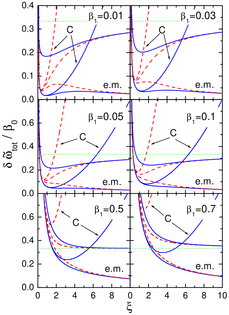
Figure 2: Fraction dependence of the effective energy per droplet volume as a function of the scaled radius $\xi=R/\lambda_{\rm D}^{\rm I}$, where $\beta_{0}$ is the parameter of the energy scale and $\beta_{1}$ is the parameter proportional to the surface tension, see (72), (73). Solid lines are given for $f=0.5$ and dashed lines for $f=1/100$. The Coulomb curves “C” are calculated with the help of eqs (144), (149), demonstrating the Coulomb limit, and “e.m.” curves relate to “the electric field energy” plus surface energy (without “correlation” contributions), $\alpha_{0}=\lambda_{\rm D}^{\rm I}/\lambda_{\rm D}^{\rm II}$ is fixed as $\alpha_{0}=1$.

In Fig. 2 we demonstrate the dependence of the contribution of the inhomogeneous charge distributions to the total thermodynamic potential per droplet volume for the case of the lattice of spherical droplets, $\delta\widetilde{\omega}_{\rm tot}/\beta_{0}=(\widetilde{\epsilon}_{V}^{\rm I}+\widetilde{\epsilon}_{V}^{\rm II}+\widetilde{\omega}_{\rm cor}^{\rm I}+\widetilde{\omega}_{\rm cor}^{\rm II}+\widetilde{\epsilon}_{\rm S})/\beta_{0}$, given by the sum of partial contributions (62), (5.2.1), (5.2.1), (66) and (71), if $\kappa^{\rm II}R_{\rm W}>1$, and by the sum of (67), (5.2.2), (5.2.2), (70) and (71), if $\kappa^{\rm II}R_{\rm W}<1$. It is presented as the function of the droplet size ($\xi$ in dimensionless units) for two values of the Wigner-Seitz parameter $f^{\rm I}\equiv f=0.01$ (dashed curves) and $f=0.5$ (solid curves) at fixed value $\beta_{1}$ (each panel) for $\alpha_{0}=1$, as the representative example. The curves for $f=0.01$ deviate only little from those for $f\rightarrow 0$ related to the single droplet.

The curves labeled by “C”, the Coulomb curves, demonstrate the contribution in the Coulomb limit: $\widetilde{\epsilon}_{{\rm C},\rm S}/\beta_{0}$ is determined by eq. (74) for $f\rightarrow 0$ and by eqs. (144), (149) in general case, dashed curves stand for $f=0.01$ and solid ones, for $f=0.5$. Each “C” curve has a pronounced minimum at $\xi=\xi_{\rm min}\propto\beta_{1}^{1/3}$. For $\xi>\xi_{\rm min}$ the “C” curve shows quadratic growth deviating drastically for $\xi\stackrel{{\scriptstyle\scriptstyle>}}{{\phantom{}{}_{\sim}}}1$ from the other curves.

The dashed and solid “e.m.” curves shown in each panel demonstrate the contribution $\widetilde{\epsilon}_{\rm e.m.}/\beta_{0}\equiv(\widetilde{\epsilon}_{V}+\widetilde{\epsilon}_{\rm S})/\beta_{0}$ for $f=0.01$ and $f=0.5$ respectively, ignoring correlation terms. The quantity $\widetilde{\epsilon}_{\rm e.m.}$ for $f\rightarrow 0$ is the counterpart of that in the Coulomb limit of $\widetilde{\epsilon}_{\rm C,S}$, when the charge screening effect is taken into account. We see that the minima at the ”e.m.” curves disappear already at $\beta_{1}>0.03$.

For $\beta_{1}\stackrel{{\scriptstyle\scriptstyle<}}{{\phantom{}{}_{\sim}}}0.01$, minimum points of the dashed “C” curves $\xi_{\rm min}$ deviate little from the minima of the dashed “e.m.” curves. Only for such small values of $\beta_{1}$ and $\xi_{\rm min}$ we recover the Coulomb limit! However, one may obtain such small values of $\beta_{1}$ only for tiny values of the surface tension and very large values of the baryon chemical potential. With increase of the latter, the Debye screening parameter $\kappa^{\rm I}$ is also increased and the droplet radius $R_{\rm min}=\xi_{\rm min}/\kappa^{\rm I}$ is proved to be essentially smaller than $1/m_{\pi}$. For larger values of $\beta_{1}$, the difference between the minima of the dashed “e.m.” and the dashed “C” curves is proved to be more pronounced. The difference between the minima at the dash “C” and dashed curves ( $\delta\widetilde{\omega}_{\rm tot}/\beta_{0}$) for the case of a tiny quark fraction volume ($f=0.01$) is minor for $\beta_{1}\stackrel{{\scriptstyle\scriptstyle<}}{{\phantom{}{}_{\sim}}}0.05$ but becomes pronounced for larger values $\beta_{1}$, whereas for the solid curves ($f=0.5$) this difference is always pronounced, even for very small $\beta_{1}$. The latter is due to an essential contribution of the correlation effective energy in this case ($f=0.5$), whereas $\rho^{\rm I}_{\rm ch}$ is fitted by coincidence of the “C” and its generic partner the “e.m.” curve in the limit $\xi\ll 1$. In the framework of the Coulomb limit the value $\rho^{\rm I}_{\rm ch}$ is defined in the variational procedure: the total energy is assumed to be dependent on $\rho^{\rm I}_{\rm ch}$ via $f$ and $\rho^{\rm I}_{\rm ch}$ is determined by the minimization of the energy. Then mentioned discrepancy could be partially diminished. However even by normalizing the solid “C” curve to coincide with the solid curve at $\xi\ll 1$ (for that please simply do the shift of the minimum at the solid “C” curve up to the value given by the minimum at the solid curve in the panel $\beta_{1}=0.01$ and use the same value of the shift considering other panels) we obtain that the difference between the minima at the curves (which determine droplet radii) becomes pronounced for $\beta_{1}>0.05$. This difference is more pronounced for $\alpha_{0}\neq 1$.

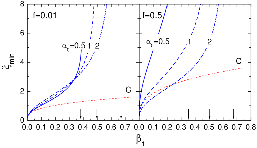
Figure 3: The radius $\xi_{\rm min}=R_{\rm\min}/\lambda_{\rm D}^{\rm I}$ of the spherical droplet corresponding to the minimum of the effective energy, $\delta\widetilde{\omega}_{\rm tot}$, in dimensional units. The “C” curves are presented for $\alpha_{0}=1$, as in Fig. 2.

The dashed and solid curves converge to $1/3$ with the increase of $\xi$. The large $\xi$ asymptotic of the curves (counted from $1/3$) is $\propto 1/\xi$, being interpreted as the surface energy term, characterized by a significantly smaller value of the surface tension (79) than that determined only by the strong interaction. We see that for $\sigma\geq\mid\sigma_{V}\mid$, corresponding to $\beta_{1}>\beta_{1{\rm c}}\simeq 0.5$ for $\alpha_{0}=1$, see Fig.3, the structured mixed phase is proved to be prohibited, since a necessary condition of its existence (the presence of a minimum in the droplet size) is not satisfied. Contrary to this in the Coulomb limit the necessary condition is always fulfilled. Large-size droplets are realized within the mixed phase if $\sigma<\mid\sigma_{V}\mid$, $\mid\sigma+\sigma_{V}\mid\ll\mid\sigma_{V}\mid$ and within the Maxwell construction, if $\sigma\geq\mid\sigma_{V}\mid$.

The difference between the solid and dashed curves and the corresponding ”e.m” curves shows the important contribution of the correlation energy in the H-Q structured mixed phase. This correlation contribution contains two parts, the model independent constant term ($\beta_{0}/3$ in our case), as follows from (5.2.1), and a model dependent part. The latter however depends only on three parameters $\beta_{0}/3$ and $\alpha_{0}=\lambda_{\rm D}^{\rm I}$, $\lambda_{\rm D}^{\rm II}$, $f^{\rm I}$. The constant term $\beta_{0}/3$ shows a difference in the energies of the Maxwell construction and the mixed phase, if one neglected finite size effects in the calculation of the latter.

The minima of the solid “e.m.” curves are always below the corresponding minima of the dashed curves, however for the $\delta\widetilde{\omega}_{\rm tot}(\xi_{\rm min})/\beta_{0}$ at the dashed and solid curves the situation changes to the opposite one, $\delta\widetilde{\omega}_{\rm tot}(\xi_{\rm min})/\beta_{0}$ increases with $f$. Comparison of the solid and the dashed curves for $\beta_{1}\geq 0.5$ demonstrates only a minor dependence of the value $\delta\widetilde{\omega}_{\rm tot}/\beta_{0}$ on the Wigner-Seitz parameter $f$ in this case.

Fig. 3 demonstrates the dependence of the droplet radius $\xi_{\rm min}$ (in dimensionless units) on the value $\beta_{1}$ for different ratios of the Debye screening lengths $\alpha_{0}$, again for two values of the Wigner-Seitz parameter $f=0.01$ (a tiny quark concentration ) and $f=0.5$. As seen from the figure, the dependence of $\xi_{\rm min}$ on the parameter $\alpha_{0}$ is rather sharp, whereas it was completely absent for the Coulomb curves in previous works since there $\rho_{\rm ch}^{\rm I}$ was considered as a function of $f$ rather than of $\kappa^{\rm I}$ and $\kappa^{\rm II}$. The dependence on $f$ is more sharp for $\alpha_{0}<1$ and less sharp for $\alpha_{0}>1$. All the curves demonstrate the presence of a critical parameter set ($\beta_{1c},\xi_{\rm min}^{c})$. The values $\beta_{1c}$ are shown by arrows in Fig. 3, cf. with Fig. 2. Corresponding values $\xi_{\rm min}^{c}$ are rather large demonstrating that even the droplets of the size $\stackrel{{\scriptstyle\scriptstyle>}}{{\phantom{}{}_{\sim}}}10\lambda_{\rm D}^{\rm I}$ may still exist within the mixed phase. This statement disagrees with what was expected in previous works using the Coulomb solutions. It was thought that the mixed phase should disappear for $\xi>\lambda_{\rm D}$ due to the screening.

For larger values of $\beta_{1}$ ($\beta_{1}>\beta_{1c}$) the Maxwell construction becomes energetically favorable. The Coulomb curves, “C” show the value $\xi_{\rm min}$ related to the unscreened case, as the function of $\beta_{1}$, ($\xi_{\rm min}(\beta_{1})=(15\beta_{1}/4)^{1/3}$ for a tiny quark fraction volume). The necessary condition for the existence of the mixed phase (existence of $\xi_{\rm min}$) is always fulfilled in the Coulomb limit, opposite to what we find in our general consideration. Comparison of the curves with the “C” curves again demonstrates the importance of the screening effects.

6 Plane geometry

6.1 Electric field configurations in Wigner-Seitz cell.

Without incorporation of screening effects previous papers argued that with increasing of the quark fraction volume the lattice of spherical droplets first undergoes the phase transition transforming to the structure of rods and then to the structure of slabs, which eventually become energetically more favorable compared to spherical droplets and rods at $f^{\rm I}<0.5$, cf. [16, 17]. Therefore, we will describe these configurations but now including the charge screening effects. We will concentrate on discussion of slabs, since in absence of screening effects, as has been shown in mentioned works, these structures appear already at sufficiently small quark fraction volume, and also, since in this case we may easily proceed further with our analytical approach.

Let the quark slab occupies a layer $x\in(-R,R)$, $-\infty<y,z<+\infty$, being placed in the Wigner-Seitz cell $x\in(-R_{\rm W},R_{\rm W})$, $R_{\rm W}\geq R$. We suppose that in the interval $x\in(-R,R)$ the electric potential well $V$ is an even function of $x$. Also we assume that the solutions of eq. (19) should not change under simultaneous replacements $x\rightarrow-x$, $R\rightarrow-R$, $R_{\rm W}\rightarrow-R_{\rm W}$. For the charged density (4), dropping the terms $\sim O(V^{2}(x))$, we easily find a solution of (19)

$$V^{\rm I}(x)-\mu_{e}=V_{0,\rm I}^{(1)}\mbox{ch}(\kappa^{\rm I}x)+U_{0}^{\rm I},\,\,\,-R<x<R.$$ (80)

Here, by superscript $(1)$ we indicate the flat geometry of the structure, $V_{0,\rm I}^{(1)}$ is an arbitrary constant and the values $\kappa^{\rm I}$, and $U_{0}^{\rm I}$ are determined by eq. (43), as in the case of the spherical geometry.

The solution of (19), $V^{\rm II}(x)=V_{0}^{\rm II}+\delta V^{\rm II}(x)$, $V_{0}^{\rm II}=const$, $\mid\delta V^{\rm II}(x)\mid\ll\mid V_{0}^{\rm II}\mid$ for $R<x<R_{\rm W}$, with the boundary condition $V^{\prime}_{x}(x=R_{\rm W})=0$, reads

$$V^{\rm II}(x)-\mu_{e}=V_{0,\rm II}^{(1)}\mbox{ch}(\kappa^{\rm II}(x-R_{\rm W}))+U_{0}^{\rm II},\,\,\,R<x<R_{\rm W},$$ (81)

where $V_{0,\rm II}^{(1)}$ is an arbitrary constant and the values $\kappa^{\rm II}$ and $U_{0}^{\rm II}$ are determined by the same equations, as in the case of the spherical geometry. The corresponding solution (19) for $-R_{\rm W}<x<-R$, with the boundary condition $V^{\prime}_{x}(x=-R_{\rm W})=0$ renders

$$V^{\rm II}(x)-\mu_{e}=V_{0,\rm II}^{(1)}\mbox{ch}(\kappa^{\rm II}(x+R_{\rm W}))+U_{0}^{\rm II},\,\,\,-R_{\rm W}<x<-R.$$ (82)

Matching of potentials and their derivatives at $x=\pm R$ yields

$$V_{0,\rm I}^{(1)}=\frac{(U_{0}^{\rm II}-U_{0}^{\rm I})\alpha_{0}}{\alpha_{0}\mbox{ch}\xi+\mbox{sh}\xi\mbox{cth}(\alpha_{2}\xi)},$$ (83)

$$V_{0,\rm II}^{(1)}=-\frac{(U_{0}^{\rm II}-U_{0}^{\rm I})\mbox{th}\xi}{\alpha_{0}\mbox{sh}(\alpha_{2}\xi)+\mbox{th}\xi\mbox{ch}(\alpha_{2}\xi)},$$ (84)

where for one dimensional structures the parameter $\alpha_{1}$ is replaced by $\alpha_{2}=\alpha_{0}(1-f^{\rm I})/f^{\rm I}$, $f^{\rm I}=R/R_{\rm W}$.

Boundary conditions for $x=-R,x=-R_{\rm W}$ are automatically fulfilled. The solution describing a tiny quark fraction volume, when one may deal with a single slab, is obtained from here in the limit $R_{\rm W}\rightarrow\infty$.

6.2 Effects of charge inhomogeneity in energy and thermodynamic potential

Using (80), (83), we first find contribution to the energy per slab from the term $\epsilon_{V,\rm I}^{(1)}$:

$$\widetilde{\epsilon}_{V,\rm I}^{\,(1)}=\frac{1}{2R}\int_{-R}^{R}\frac{(\nabla V(x))^{2}}{8\pi e^{2}}dx=\beta_{0}\frac{\mbox{th}^{2}(\alpha_{2}\xi)\left(\mbox{th}^{2}\xi-1+\frac{1}{\xi}\mbox{th}\xi\right)}{6\left(\alpha_{0}^{-1}\mbox{th}\xi+\mbox{th}(\alpha_{2}\xi)\right)^{2}}.$$ (85)

Using eqs (81), (84), we then obtain the term $\epsilon_{V,\rm II}^{(1)}$:

$$\widetilde{\epsilon}_{V,\rm II}^{\,(1)}=\frac{1}{R}\int_{R}^{R_{\rm W}}\frac{(\nabla V(x))^{2}}{8\pi e^{2}}dx$$

$$=\beta_{0}\frac{\mbox{th}^{2}\xi\left(\frac{1}{\alpha_{0}\xi}\mbox{th}(\alpha_{2}\xi)+\frac{\alpha_{2}}{\alpha_{0}}\left(\mbox{th}^{2}(\alpha_{2}\xi)-1\right)\right)}{6\left(\alpha_{0}^{-1}\mbox{th}\xi+\mbox{th}(\alpha_{2}\xi)\right)^{2}}.$$ (86)

For $\widetilde{\omega}_{\rm cor,I}^{(1)}$, with the help of eqs (30), (80) and (43) taking $V_{\rm ref}^{\rm I}=V^{\rm bulk}$ we find

$$\widetilde{\omega}_{\rm cor,I}^{\,(1)}=\frac{1}{2R}\int_{-R}^{R}dx\omega_{\rm cor,I}^{(1)}=\beta_{0}\frac{\mbox{th}^{2}(\alpha_{2}\xi)\left(1-\mbox{th}^{2}\xi+\frac{1}{\xi}\mbox{th}\xi\right)}{6\left(\alpha_{0}^{-1}\mbox{th}\xi+\mbox{th}(\alpha_{2}\xi)\right)^{2}}$$

$$-\beta_{0}\frac{2\mbox{th}(\alpha_{2}\xi)\mbox{th}\xi}{3\xi\left(\alpha_{0}^{-1}\mbox{th}\xi+\mbox{th}(\alpha_{2}\xi)\right)}+\frac{\beta_{0}}{3}.$$ (87)

Using eqs (30), (81), (48) and taking $V_{\rm ref}^{\rm II}=V^{\rm bulk}$, we obtain

$$\widetilde{\omega}_{\rm cor,II}^{(1)}=\frac{1}{R}\int_{R}^{R_{W}}dx\omega_{\rm cor,II}^{(1)}$$ (88)

$$=\beta_{0}\frac{\mbox{th}^{2}\xi\left[\frac{1}{\xi}\mbox{th}(\alpha_{2}\xi)+\alpha_{2}\left(1-\mbox{th}^{2}(\alpha_{2}\xi)\right)\right]}{6\alpha_{0}\left(\alpha_{0}^{-1}\mbox{th}\xi+\mbox{th}(\alpha_{2}\xi)\right)^{2}}.$$

The surface energy contribution per slab is given by

$$\widetilde{\epsilon}_{\rm S}^{(1)}=\frac{\beta_{0}\beta_{1}}{3\xi},$$ (89)

see eq. (112) of Appendix B.

Tiny quark fraction volume. Single slab.

Expressions for a single slab are obtained taking the limit $R_{\rm W}\rightarrow\infty$ ($\alpha_{2}\rightarrow\infty$).

Slab of a tiny transverse size.

The solution for a single slab of a tiny transverse size is recovered for $\xi\ll 1$, $\alpha_{2}\xi\gg 1$. This limit is never realized for an unscreened slab, the potential of which is linearly growing for $x\rightarrow\pm\infty$. In the realistic case under consideration any charged slab is screened already at distances $\sim 1/\lambda_{\rm D}^{\rm II}$ from it. Then, the main contribution to the energy per slab comes from the terms $\widetilde{\epsilon}_{V,\rm II}^{\,(1)}\simeq\widetilde{\omega}_{\rm cor,II}^{(1)}\propto\xi$. The term $\widetilde{\epsilon}_{V,\rm I}^{\,(1)}$ is $\propto\xi^{2}$, and $\widetilde{\omega}_{\rm cor,I}^{\,(1)}\propto\xi^{3}$. In this limit, i.e. for a tiny quark fraction volume, we immediately obtain that unscreened spherical droplets are energetically more favorable compared to slabs. Indeed, we have

$$\widetilde{\epsilon}_{\rm C,S}^{(1)}\simeq\frac{\beta_{0}\xi}{3\alpha_{0}}+\frac{\beta_{0}\beta_{1}}{3\xi},$$ (90)

from where we find the minimum $\xi_{\rm min}=\sqrt{\alpha_{0}\beta_{1}}$ and $\widetilde{\epsilon}_{\rm C,S}^{(1)}(\xi_{\rm min})=2\widetilde{\epsilon}_{\rm C}(\xi_{\rm min})=\frac{2}{3}\beta_{0}\sqrt{\beta_{1}/\alpha_{0}}$, that is larger than the term (76) for the case of the spherical droplet ($\widetilde{\epsilon}_{\rm C,S}(\xi_{\rm min})\propto\beta_{1}^{2/3}$) for $\beta_{1}<0.11/\alpha_{0}^{3}$. This statement holds in the limit $\beta_{1}\alpha_{0}\ll 1$ and $f^{\rm I}\ll\alpha_{0}(\beta_{1}\alpha_{0})^{1/2}$ corresponding to $\xi_{\rm min}\ll 1$ and $\alpha_{2}\xi_{\rm min}\gg 1$ for slabs, and $\beta_{1}\ll 1$, $\alpha_{0}^{3}\beta_{1}\gg f^{\rm I}$ corresponding to $\xi_{\rm min}\ll 1$ and $\alpha_{1}\xi_{\rm min}\gg 1$ for droplets, accordingly.

Slab in Wigner-Seitz cell, both of tiny transverse sizes.

This limit is recovered for $\xi\ll 1$, $\alpha_{2}\xi\ll 1$. Then we arrive at expressions

$$\widetilde{\epsilon}_{V,\rm I}^{(1)}=\frac{\alpha_{0}^{2}\alpha_{2}^{2}\beta_{0}\xi^{2}}{9(1+\alpha_{0}\alpha_{2})^{2}},\,\,\,\ \widetilde{\epsilon}_{V,\rm II}^{(1)}=\frac{\alpha_{0}\alpha_{2}^{3}\beta_{0}\xi^{2}}{9(1+\alpha_{0}\alpha_{2})^{2}},$$ (91)

$$\widetilde{\omega}_{\rm cor,I}^{(1)}=\frac{\beta_{0}}{3(1+\alpha_{0}\alpha_{2})^{2}}-\frac{2\beta_{0}\alpha_{0}\alpha_{2}^{2}(\alpha_{0}+\alpha_{2})}{9(1+\alpha_{0}\alpha_{2})^{3}}\xi^{2},$$ (92)

$$\widetilde{\omega}_{\rm cor,II}^{(1)}=\frac{\beta_{0}\alpha_{0}\alpha_{2}}{3(1+\alpha_{0}\alpha_{2})^{2}}+\frac{2\beta_{0}\alpha_{0}\alpha_{2}^{2}(\alpha_{0}+\alpha_{2})}{9(1+\alpha_{0}\alpha_{2})^{3}}\xi^{2},$$

and thus $\widetilde{\omega}_{\rm cor,I}^{(1)}+\widetilde{\omega}_{\rm cor,II}^{(1)}\simeq\frac{1}{3}\beta_{0}(1+\alpha_{0}\alpha_{2})^{-1}$.

Summation of all the terms (91), (92) together with (89) yields, after minimization over $\xi$:

$$\widetilde{\omega}_{\rm tot}^{(1)}(\xi_{\rm min})/\beta_{0}=\frac{\beta_{1}^{2/3}\alpha_{0}(1-f^{\rm I})^{1/3}}{3^{1/3}2^{2/3}[\alpha_{0}^{2}+f^{\rm I}(1-\alpha_{0}^{2})]^{2/3}}+\frac{f^{\rm I}}{3[\alpha_{0}^{2}+f^{\rm I}(1-\alpha_{0}^{2})]},$$ (93)

where we used that

$$\xi_{\rm min}=\left(\frac{3\beta_{1}[\alpha_{0}^{2}+f^{\rm I}(1-\alpha_{0}^{2})]^{2}}{2\alpha_{0}^{3}(1-f^{\rm I})}\right)^{1/3}\ll 1,$$ (94)

and $\alpha_{2}\xi_{\rm min}\ll 1$, that corresponds to $(\beta_{1}\alpha_{0})^{1/3}\ll 1$ and $f^{\rm I}\gg\alpha_{0}(\beta_{1}\alpha_{0})^{1/3}$.

Single slab of large transverse size.

As follows from eqs (85) - (89), in the limit of a single large slab of a much larger transverse size than the typical Debye screening lengths ($\xi\gg 1$, $\alpha_{2}\xi\gg 1$), all the terms contribute to the surface energy per slab with the corresponding surface tension terms $\sigma^{(1)}_{i}=\sigma^{\rm spher}_{i}$, and, thus, for the total surface tension we get $\sigma^{(1)}_{\rm tot}=\sigma^{\rm spher}_{\rm tot}$.

The slab of a large transverse size has three times smaller negative contribution to the surface energy per slab than that for the corresponding spherical droplet in case $\sigma^{(1)}_{\rm tot}<0$, when the mixed phase is energetically favorable. Here, the factor three comes from the space dimension. Thus, droplets are energetically favorable compared to slabs also in this limit.

For the case $\sigma^{(1)}_{\rm tot}>0$ realized within the Maxwell construction the plane boundary layer is energetically preferable. In spite of that, in any case the boundary layer, which arises between two separate phases within the Maxwell construction, is spherical, following the geometry of the neutron star as a whole. Above discussed slabs could exist in the neutron star only, as configurations of the mixed phase, being rather small in their transverse sizes.

6.3 Numerical results

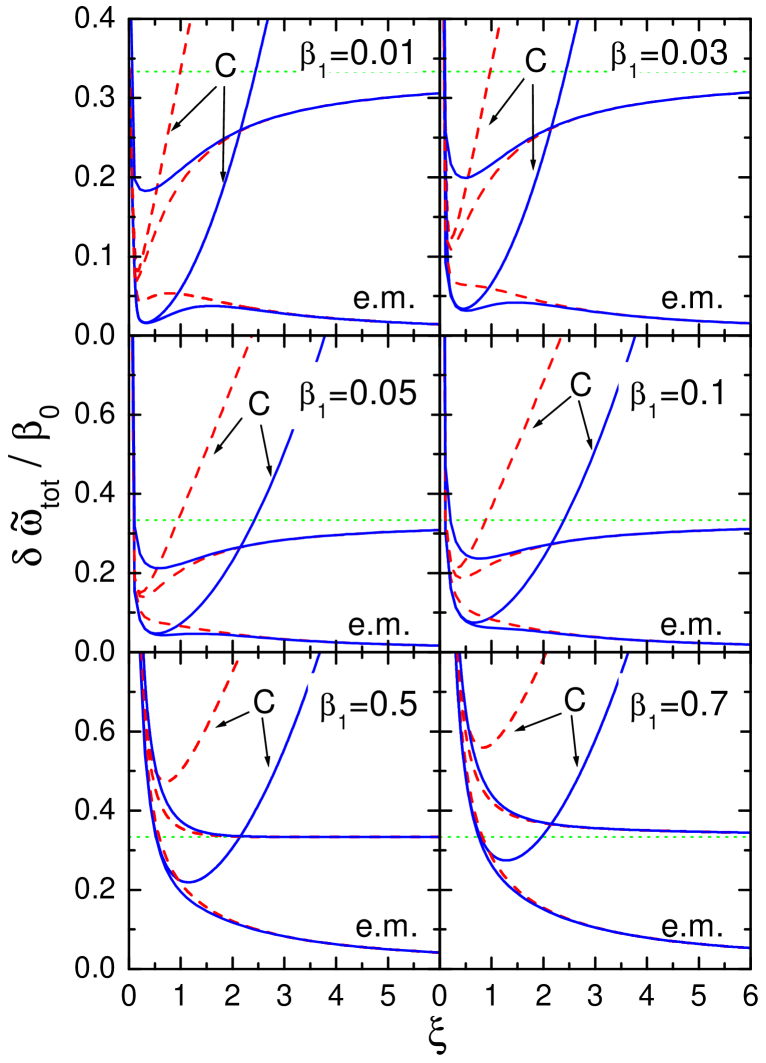
Figure 4: The same, as in Fig. 2, but for slabs. The curves labeled by “C” are calculated with the help of eq. (90) for $f=0.01$ (dashed) and (145), (149) for $f=0.5$ (solid).

In Fig. 4 we show the same quantity, $\delta\widetilde{\omega}_{tot}/\beta_{0}$, as in Fig. 2, but now for slabs, for the values of the Wigner-Seitz parameter $f\equiv f^{\rm I}=0.01$ and $f=0.5$, and for the parameter $\alpha_{0}=1$. The “C” curves are calculated with the help of eq. (90) for $f=0.01$ (dashed) and eqs (145), (149) of Appendix E for $f=0.5$ (solid). Eq. (145) gives a divergent result in the limit $f\rightarrow 0$ and is not applicable to describe single slab of a tiny transverse size.

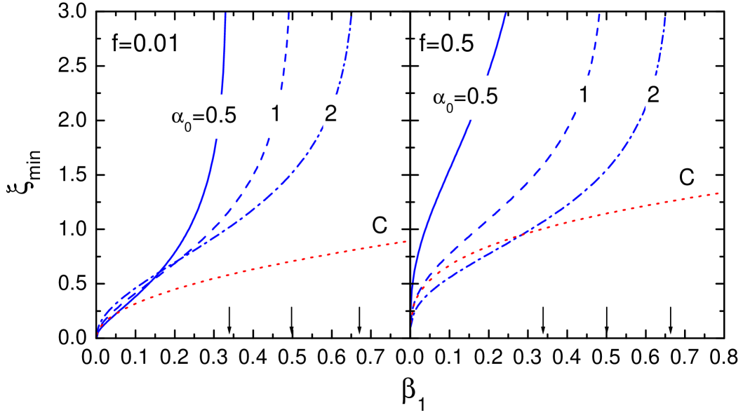
Figure 5: The transverse slab radius $\xi_{\rm min}$ corresponding to the minimum of the effective energy, $\delta\widetilde{\omega}_{\rm tot}^{(1)}$, in dimensionless units. The “C” curves are the same, as in Fig. 4, shown for $\alpha_{0}=1$.

Difference between the non-labeled curves ($\delta\widetilde{\omega}_{tot}^{(1)}/\beta_{0}$) and the ”e.m.” curves shows how large are correlation terms. We see that forms of all the curves are analogous to those for the spherical droplet case. Minima disappear at the “e.m.” curves already for $\beta_{1}\geq 0.03$ at $f=0.01$ and for $\beta_{1}\geq 0.05$ at $f=0.5$. Minima of the non-labeled curves ($\delta\widetilde{\omega}_{tot}^{(1)}/\beta_{0}$) disappear at $\beta_{1}>0.5$ for both $f=0.01$ and $f=0.5$ cases, cf. Fig. 5.

The dashed ”C” curve is the appropriate limit of the dashed curve ($\delta\widetilde{\omega}_{tot}^{(1)}/\beta_{0}$) at a tiny $f$ and $\xi\ll 1$. It grows linearly with $\xi$. At their minima the dashed ”C” curves begin to essentially deviate from the minima of the corresponding dashed curves for $\beta_{1}\stackrel{{\scriptstyle\scriptstyle>}}{{\phantom{}{}_{\sim}}}0.05\div 0.1$. If they were normalized to coincide with the “e.m.” dashed curves at a tiny $\beta_{1}$, their minima would be shifted down by factor $1/\sqrt{2}$ since $\widetilde{\epsilon}_{V,\rm II}^{\,(1)}\simeq\widetilde{\omega}_{\rm cor,II}^{\,(1)}\propto\xi$, and $\widetilde{\epsilon}_{V,\rm I}^{\,(1)}\propto\xi^{2}$ and $\widetilde{\omega}_{\rm cor,I}^{\,(1)}\propto\xi^{3}$ are neglected. Solid “C” curves ($f=0.5$) are normalized to coincide with the corresponding “e.m.” curve for $\xi\ll 1$, see discussion in Appendix E.

Fig. 5 demonstrates the dependence of the slab size in dimensionless units, $\xi_{\rm min}$, on the parameter $\beta_{1}$ for $f=0.01$ and $f=0.5$, for three values of $\alpha_{0}$, cf. with Fig. 2 for the spherical droplet case. The $\alpha_{0}$ dependence is here even stronger than for the spherical geometry. Also the transverse size of the slab is smaller.

7 Comparison of energies of droplets and slabs

As has been argued in the previous studies, cf. [8] sect. 4.3.1, the bulk energy densities of the quark and hadron phases are about two orders of magnitude larger than the sum of the Coulomb and surface energies. This large factor is partially due to the fact that the latter sum contains an extra $\propto e^{2/3}$ pre-factor compared to the energy densities of the bulk phases given by eqs (95) and (96) of Appendix A. One can see this pre-factor after minimization of the sum of the surface and the Coulomb energy densities with respect to $R$, taking into account that the values $\rho_{\rm ch}^{\rm I,II}$ entering eq. (142) of Appendix E do not contain this pre-factor and that the resulting surface energy density is of the order of the Coulomb one. An extra small factor arises from the smallness of the difference $\rho_{\rm ch}^{\rm I}-\rho_{\rm ch}^{\rm II}$ entering eq. (142).

With our screened potentials, the smallness of the value $\delta\widetilde{\omega}_{\rm tot}(\xi_{\rm min})$ is due to the parameter $\beta_{1}\propto e$ (cf. eq. (73)) for typical values $\xi_{\rm min}\stackrel{{\scriptstyle\scriptstyle>}}{{\phantom{}{}_{\sim}}}1$.

¿From the Figs 1 - 5 and eqs. (95) and (96) of Appendix A we may see that typically $\delta\widetilde{\omega}_{\rm tot}(\xi_{\rm min})$ (with $\xi_{\rm min}$ essentially dependent on the geometry of the structure) is at least by an order of magnitude smaller than the bulk values of the energy densities. This justifies the same “two part approach” to the problem, as has been used in previous papers of Glendenning and his co-authors, of computing first the bulk properties and then on this background, the geometrical structure imposed by the effective energy $\delta\widetilde{\omega}_{\rm tot}(\xi_{\rm min})$.

The bulk structure is defined following the strategy, sketched in [8], sect. 4.1.3. Begin with solving the equations that define quantities of the phase II using the local charge neutrality condition and increasing the baryon density. At each baryon density find the values of the chemical potentials $\mu_{B,\rm loc}^{\rm II}$ and $\mu_{e,\rm loc}^{\rm II}$. At each density also find the solution of the high-density phase I at the very same value of the chemical potentials thus putting $\mu_{B,\rm loc}^{\rm II}=\mu_{B,\rm Gibbs}=const$ and $\mu_{e,\rm loc}^{\rm II}=\mu_{e,\rm Gibbs}=const$ and using the relations (34) - (36). Locate the value of the chemical potentials for which the pressures in the two phases are equal. The beginning point of the mixed phase is fixed in this way. The complementary procedure will locate the boundary between the mixed phase and the pure phase I (quark phase). Then we may find the properties of the mixed phase in which both phases are present in equilibrium. To find the volume fraction of phase II at fixed $\rho_{B}$, for given $f$ (starting from infinitely small $f$) solve the equations defining both phases subject to the conditions of equal pressure and global charge neutrality, where the charged densities are defined through the values of the corresponding constant chemical potentials which, as well as the pressure, vary with $f$. The value $f$ is a function of $\rho_{B}$, see (5). The increase of the value $f$ corresponds to the increase of the baryon density (5). The value $f=1$ corresponds to the end point of the mixed phase.

Then, in order to define, which geometrical structure is energetically favorable, we may use the values of $\rho_{B}$ and $f$ thus calculated, and compare the quantities $\delta\widetilde{\omega}_{\rm tot}^{(d_{1})}(\xi_{\rm min}^{(d_{1})})$ and $\delta\widetilde{\omega}_{\rm tot}^{(d_{2})}(\xi_{\rm min}^{(d_{2})})$. The latter values relate to the distinct possible configurations (quark/hadron) of different geometries $d_{1}$ and $d_{2}$. As we have mentioned, in the present paper we restrict ourselves to the consideration of the quark structures embedded into hadron matter for $f\leq 0.5$ and by studying of the two geometries $d_{1}=3$ (spherical quark droplets) and $d_{2}=1$ (quark slabs). Each quantity $\delta\widetilde{\omega}_{\rm tot}^{(3)}(\xi_{\rm min}^{(3)})$ and $\delta\widetilde{\omega}_{\rm tot}^{(1)}(\xi_{\rm min}^{(1)})$ is minimized with respect to the structure size ($\xi_{\rm min}^{(3)}$ and $\xi_{\rm min}^{(1)}$). The values $\xi_{\rm min}^{(3)}$ and $\xi_{\rm min}^{(1)}$ are, thereby, essentially different, see Figs 3 and 5. This is due to the fact that the minimization in $\xi$ is performed for the quantities $\delta\widetilde{\omega}_{\rm tot}^{(3)}(\xi)$ and $\delta\widetilde{\omega}_{\rm tot}^{(1)}(\xi)$, being of the same order of magnitude (having the same $e$ pre-factors). Thus the argument which allowed us to fix $f$ to be the same for both structure geometries does not hold for $\xi$. As we have demonstrated above, cf. Figs 3, 5, the minima $\xi_{\rm min}^{(1)}$ and $\xi_{\rm min}^{(3)}$ exist not for all values of $\beta_{1}$, but only for those related to not too large values of the surface tension parameter. Otherwise the presence of the mixed phase is not energetically favorable compared to the configuration given by the Maxwell construction.

Above procedure implies that the corrections to $f$ due to its dependence on the geometrical structure and accordingly on the values of $\xi_{\rm min}^{(1)}$ or $\xi_{\rm min}^{(3)}$ are rather small. Therefore they are neglected. The values of $\rho_{\rm ch}^{\rm I,II}$ used in determining the parameters of the inhomogeneous spatial structures, should not be constants in the general case, rather they are now functions of $\vec{r}$ given by (4) and (40). The global charge neutrality condition is now satisfied since we use the boundary condition $\nabla V=0$ at the boundary of the Wigner - Seitz cell.

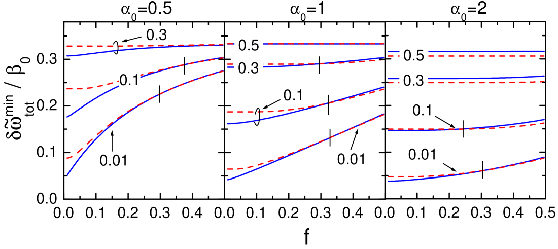
Figure 6: Comparison of the effective energies of droplets (solid curves) and slabs (dashed curves). The numbers at the curves are the values of $\beta_{1}$. Crossing points of the curves are indicated.

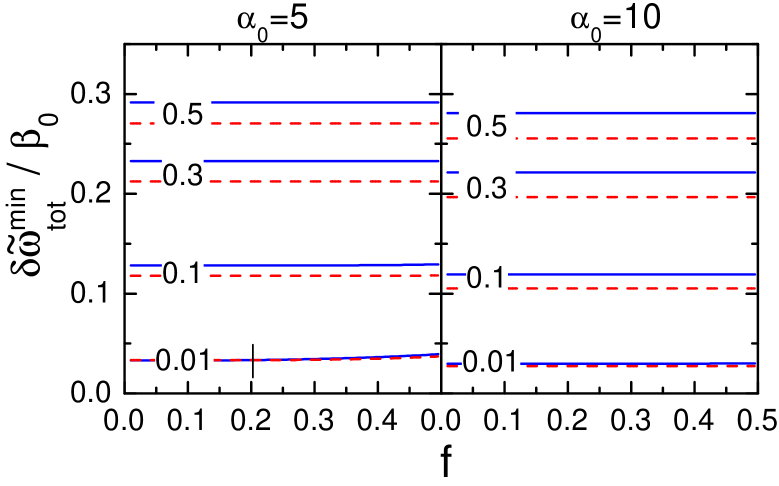
Figure 7: The same, as in Fig. 6, but for large values of $\alpha_{0}$.

Fig. 6 shows which structures (spheres or slabs) are more energetically favorable for the given value of the parameter $f$, in dependence on the value of $\beta_{1}$. The solid curves, $\delta\widetilde{\omega}_{\rm tot}^{\rm min}/\beta_{0}\equiv\delta\widetilde{\omega}_{\rm tot}^{(3)}(\xi_{\rm min}^{(3)})/\beta_{0}$, present droplets and the dashed curves, $\delta\widetilde{\omega}_{\rm tot}^{\rm min}/\beta_{0}\equiv\delta\widetilde{\omega}_{\rm tot}^{(1)}(\xi_{\rm min}^{(1)})/\beta_{0}$, the slabs. The result, which structure is energetically favorable, essentially depends on the values of parameters $\alpha_{0}$ and $\beta_{1}$. For $\alpha_{0}=0.5$, $\beta_{1}\stackrel{{\scriptstyle\scriptstyle>}}{{\phantom{}{}_{\sim}}}0.3$ spherical droplets are energetically favored for any value of the parameter $f<0.5$. For $\alpha_{0}=2$, $\beta_{1}\stackrel{{\scriptstyle\scriptstyle>}}{{\phantom{}{}_{\sim}}}0.3$ slabs are energetically favored. For unrealistically large values of $\alpha_{0}$, see the cases $\alpha_{0}=5;10$ in Fig. 7, we find that slabs become to be energetically favorable structures already for $\beta_{1}\stackrel{{\scriptstyle\scriptstyle>}}{{\phantom{}{}_{\sim}}}0.01$. It occurs then for any $f$. Our conclusions here essentially differ from those derived in the Coulomb limit, if one ignored the screening effects for any $\beta_{1}$ and assumed the step-function charge-density profiles. In the latter case the droplet phase is proven to be energetically favorable for $f<f_{c}^{\rm rod}\simeq 0.2$, as has been shown in ref. [16, 29]. Then for $f_{c}^{\rm rod}<f<f_{c}^{\rm slab}\simeq 0.32$ rods are prefered and for $f>f_{c}^{\rm slab}$ slabs are prefered. We recover this limit case result from our general expressions as well, but only for tiny values of $\beta_{1}$ and $\alpha_{0}=1$, see discussion in Appendix E and Fig. 8. In the latter we present the effective energies of droplets and slabs obtained with our general expressions in case $\beta_{1}=0.001$ for several values of $\alpha_{0}$.

8 Concluding remarks

Summarizing, in this paper we have discussed the possibility of the presence of structured mixed phases at first order phase transitions in multi-component systems of charged particles. Using the thermodynamical potential as the generating functional we have developed a formalism, which allows to explicitly treat electric field effects including the Debye screening.

We have studied a “contradiction” between the Gibbs conditions and the Maxwell construction extensively discussed in previous works. We have demonstrated that this contradiction is resolved if one takes into account the difference in the treatment of the chemical potentials used in the two approaches. The different values of the electron chemical potentials in the Maxwell construction and the ones used in the Gibbs conditions do not contradict each other if one takes into account the electric field arising at the boundaries of the finite size structures of the mixed phase and at the boundary between phases within the Maxwell construction.

As an example, our formalism was applied to the hadron-quark structured mixed phase. Using a linearization procedure we analytically solved the Poisson equation for the electric potential and found the electric field profiles of the structured mixed phase in cases of spherical and one-dimensional geometries. We have demonstrated that the charge screening effect greatly modifies the description of the mixed phase, changing its parameters and affecting the possibility of its existence. With screening effects included it has been proven that the mixed phase structures may exist even if their sizes are significantly larger than the Debye screening lengths. The characteristics of the structures essentially depend on the value of the ratio of the Debye screening lengths in the interior and exterior of the structure and on the value of the surface tension on its boundary. We showed the important role played by the correlation energy terms omitted in previous works. For realistic values of the parameters these correlation contributions are larger than the electromagnetic contribution to the energy discussed in previous works.

The result, which structure is energetically favorable, essentially depends on the values of parameters $\alpha_{0}$ and $\beta_{1}$. This our conclusion essentially differs from that was previously done for the Coulomb case, when one ignored the screening effects for any $\beta_{1}$ and assumed the step-function charge-density profile. We recover that limit case result from our general expressions as well, but only for tiny values of $\beta_{1}$ and $\alpha_{0}=1$.

We support the conclusion of [16, 17] that the mixed phase may arise only if the surface tension is smaller than a critical value. We also evaluated the surface tension between the hadron and the quark phases. However this evaluation remains rather rough. An uncertainty in the value of the surface tension does not allow to conclude whether the mixed H-Q phase exists or not. Both possibilities, the mixed phase and the Maxwell construction, can be studied within different models. An advantage of our study is that the characteristics of the mixed phase are expressed in terms of only few parameters. Thus knowing these parameters for a given model one may apply our results for the discussion of the mixed phase, the Maxwell construction, the geometry of the structures, the energy contributions of the structures and the electric field profiles.

In absence of a mixed phase our charged distributions describe the boundary layer between two separated phases existing within the double-tangent (Maxwell) construction. The previously obtained Coulomb limits (when one omitted the screening effects) are naturally recovered from our general expressions but only in the limiting case of tiny size droplets. This limiting case, however, is never realized for realistic values of the parameters.

In this paper we considered only droplets and slabs and their interplay for $f<0.5$ at zero temperature. More detailed analysis of a possible interplay between different structures within the whole interval $0<f<1$ and at finite temperatures will be performed in a forthcoming paper.

Acknowledgements.

Research of D.N.V. at Yukawa Institute for Theoretical Physics was sponsored by the COE program of the Ministry of Education, Science, Sports and Culture of Japan. D.N.V. acknowledges this support and kind hospitality of the Yukawa Institute for Theoretical Physics. He thanks Department of Physics at Kyoto University for the warm hospitality and also acknowledges hospitality and support of GSI Darmstadt. The present research of T.T. is partially supported by the REIMEI Research Resources of Japan Atomic Energy Research Institute, and by the Japanese Grant-in-Aid for Scientific Research Fund of the Ministry of Education, Culture, Sports, Science and Technology (11640272, 13640282). Authors greatly acknowledge E.E. Kolomeitsev for the help and discussions and M. Lutz for valuable remarks.

APPENDICES

Appendix A Energy density of quark and hadron sub-systems

In the main text, as a concrete example, we consider the H-Q phase transition. We assume that the quark matter (phase I) consists of $u,d,s$ quarks and electrons. To easier compare our results for the description of the H-Q system with those obtained previously, we choose a simple model of equation of state used in [17, 30] with slight modifications. We could use any other model. We need it here only to estimate typical values of the parameters.

The kinetic plus strong interaction energy density of the quark matter expressed in terms of particle densities is given by the bag model

$$\epsilon_{\rm kin+str}^{\rm I}\simeq\frac{3\pi^{2/3}}{4}\left(1+\frac{2\alpha_{c}}{3\pi}\right)\left[\rho_{u}^{4/3}+\rho_{d}^{4/3}+\rho_{s}^{4/3}+\frac{m_{s}^{2}\rho_{s}^{2/3}}{\pi^{4/3}}\right]+B+\frac{(3\pi^{2}\rho_{e})^{4/3}}{4\pi^{2}},$$ (95)

where $B$ is the bag constant, $\alpha_{c}$ is the QCD coupling constant, $m_{s}$ is the mass of the strange quark. Last term is the kinetic energy of electrons. Expansion is presented up to the terms linear in $\alpha_{c}$ and $m_{s}^{2}$, where the strange quark mass $m_{s}$ ($\simeq~{}$120 $\div$ 150 MeV) is supposed to be rather small compared to the quark chemical potentials, and much smaller values of $u$ and $d$ quark bare masses are omitted.

The hadron matter (phase II) in our model consists of protons, neutrons and electrons and the kinetic plus strong interaction energy density is given by

$$\epsilon_{\rm kin+str}^{\rm II}\simeq\epsilon^{n}_{\rm kin}[\rho_{n}]+\epsilon^{p}_{\rm kin}[\rho_{p}]+\epsilon_{\rm pot}[\rho_{n},\rho_{p}]+\frac{(3\pi^{2}\rho_{e})^{4/3}}{4\pi^{2}},$$ (96)

where $\epsilon^{i}_{\rm kin}[\rho_{i}],\,\,i=n,p,$ are standard relativistic kinetic energies of nucleons,

$$\epsilon^{i}_{\rm kin}=2\int\sqrt{p^{2}+m_{i}^{2}}\,n_{i}(p)\frac{d^{3}p}{(2\pi)^{3}},\,\,\,i=n,p,$$ (97)

$m_{n}\simeq m_{p}=m_{N}$ is the nucleon mass, $n_{i}(p)$ are step-functional Fermi occupations. The potential energy $\epsilon_{\rm pot}$ we take here in the form

$$\epsilon_{\rm pot}[\rho_{n},\rho_{p}] = S_{0}\frac{(\rho_{n}-\rho_{p})^{2}}{\rho_{0}}+(\rho_{n}+\rho_{p})\epsilon_{\rm bind}+\frac{K_{0}(\rho_{n}+\rho_{p})}{18}\left(\frac{\rho_{n}+\rho_{p}}{\rho_{0}}-1\right)^{2}$$ (98)

$$+ C_{\rm sat}(\rho_{n}+\rho_{p})\left(\frac{\rho_{n}+\rho_{p}}{\rho_{0}}-1\right),$$

$\rho_{0}$ is the nuclear density ($\rho_{0}\simeq 0.16$ fm^-3) and values of constants $\epsilon_{\rm bind}$, $K_{0}$, $C_{\rm sat}$ are taken to satisfy the nuclear saturation properties. The value $\epsilon_{\rm bind}=\widetilde{\epsilon}_{\rm bind}+m_{N}-2\rho_{0}^{-1}\epsilon_{p}^{kin}(\rho_{B}=\rho_{0},\rho_{p}/\rho_{B}=1/2)$ provides appropriate binding energy $\widetilde{\varepsilon}_{\rm bind}=-15.6$ MeV at the nuclear saturation density $\rho_{0}$. The coefficient $K_{0}$ is defined by the relation $K_{0}=\widetilde{K}_{0}-\frac{3p_{{\rm F}0}^{2}}{\sqrt{m_{N}^{2}+p_{{\rm F}0}^{2}}}-18C_{sat}\simeq 285$ MeV, where the value $\widetilde{K}_{0}\simeq 240$ MeV provides an appropriate compressibility at saturation. $S_{0}=\widetilde{S}_{0}-\pi^{2}\rho_{0}/(4p_{{\rm F}0}\sqrt{p_{{\rm F}0}^{2}+m_{N}^{2}})$ is the symmetry energy term. The parameter $\widetilde{S}_{0}$ is chosen to be $\widetilde{S}_{0}\simeq 30~{}$MeV, that corresponds to $S_{0}\simeq 18~{}$MeV, $p_{{\rm F}0}=p_{{\rm F}p}(\rho_{B}=\rho_{0},\rho_{p}/\rho_{B}=1/2)=p_{{\rm F}n}(\rho_{B}=\rho_{0},\rho_{p}/\rho_{B}=1/2)$ is the baryon Fermi momentum for the symmetric nuclear matter at the saturation density. The value

$$C_{sat}=2\rho_{0}^{-1}\epsilon_{p}^{kin}(\rho_{B}=\rho_{0},\rho_{p}/\rho_{B}=1/2)-\epsilon_{F0}$$ (99)

is introduced to reproduce the saturation property, $\epsilon_{{\rm F}0}=\sqrt{p_{{\rm F}0}^{2}+m_{N}^{2}}$. Higher order terms $\sim\left(\rho_{B}/\rho_{0}-1\right)^{3}$ in expansion of the potential energy are for simplicity dropped in (98), since their explicit form is not too important for our study here. Contribution of mean fields of the heavy mesons $\sigma$, $\omega$ and $\rho$ is hidden in the values of phenomenological parameters $\widetilde{K}_{0}$ and $\widetilde{S}_{0}$.

Chemical potentials of neutrons and protons are determined with the help of (95) - (98):

$$\mu_{n}=\mu_{B}=\sqrt{p_{Fn}^{2}+m_{N}^{2}}+\frac{2S_{0}(\rho_{n}-\rho_{p})}{\rho_{0}}+\epsilon_{bind}+\frac{K_{0}}{6}\left(\frac{\rho_{n}+\rho_{p}}{\rho_{0}}-1\right)^{2}$$

$$+\frac{K_{0}}{9}\left(\frac{\rho_{n}+\rho_{p}}{\rho_{0}}-1\right)+\frac{2C_{sat}(\rho_{n}+\rho_{p})}{\rho_{0}}-C_{sat},$$ (100)

$$\mu_{p}=\mu_{n}-\sqrt{p_{Fn}^{2}+m_{N}^{2}}+\sqrt{p_{Fp}^{2}+m_{N}^{2}}-\frac{4S_{0}(\rho_{B}-2\rho_{p})}{\rho_{0}}-V^{\rm II}(\vec{r}),$$

$$\mu_{e}=(3\pi^{2}\rho_{e})^{1/3}+V^{\rm II}(\vec{r}).$$

As in the phase I, $\mu_{e}=\mu_{e,\rm Gibbs}$ for $V^{0}=0$ and $\mu_{e}=0$ for $V^{0}=-\mu_{e,\rm Gibbs}$.

Varying these equations of motion, after straightforward calculations we get

$$C_{0}=\frac{\widetilde{C}_{0n}\widetilde{C}_{0p}-K_{1}(\widetilde{C}_{0p}+\widetilde{C}_{0n})}{\widetilde{C}_{0n}-K_{1}},$$ (101)

with

$$\widetilde{C}_{0j}\equiv\left[C_{0j}+\frac{4S_{0}}{\rho_{0}}\right],$$ (102)

where $C_{0j}^{-1}=p_{{\rm F}j}\sqrt{p_{{\rm F}j}^{2}+m^{2}_{j}}/\pi^{2}$ is the density of states for the given baryon species, $j=\{n,p\}$, and

$$K_{1}=\frac{2S_{0}}{\rho_{0}}-\frac{K_{0}+18C_{sat}}{9\rho_{0}}-\frac{K_{0}\rho_{B}}{3\rho_{0}^{2}}\left(1-\frac{\rho_{0}}{\rho_{B}}\right).$$ (103)

Dropping $K_{1}$ we may use a simplified expression

$$C_{0}\simeq\widetilde{C}_{0p},$$ (104)

relating to $\delta\rho_{n}(\vec{r})\simeq 0$, that is not too bad approximation for $\rho_{B}\sim\rho_{0}$ and for $\rho_{B}\gg\rho_{0}$, $p_{Fn}\gg p_{Fp}$. We use this simplified expression for rough numerical estimates.

Appendix B Surface energy of H-Q interface

The surface layer separating quark and hadron sub-systems is very difficult to describe microscopically mainly due to absence of the microscopic treatment of the confinement problem. A simplification comes from the fact that gradients of all the fields except the electric field are very sharp and this layer can be then treated in terms of surface quantities. Thus, in our consideration below we will use the fact that in absence of electric field effects the surface layer is characterized by a shortest scale $d_{\rm S}$ ($\stackrel{{\scriptstyle\scriptstyle<}}{{\phantom{}{}_{\sim}}}1$ fm as we estimate). With this, we explicitly include electric field and calculate corrections to all the meson-nucleon fields due to electric field effects. These corrections, relate to larger scales $\lambda_{\rm D}^{\rm I,II}\sim(5\div 10)$ fm corresponding to the Debye screening of the electric field. Due to that $\lambda_{\rm D}^{\rm I,II}\gg d_{\rm S}$, the electric field effects do not significantly affect the quantities related to the shortest scale $d_{\rm S}$.

Let us first discuss the case of the quark-vacuum interface. The quark contribution to the energy density of this layer arises due to sharp spatial gradients of the quark-gluon fields within the confinement area ($\delta r\sim d_{\rm S}^{\,q}\simeq 0.2\div 0.4~{}$ fm) near the bag surface. Since $d_{\rm S}^{\,q}$ is substantially smaller than the corresponding length scales $\lambda_{\rm D}^{\rm I,II}$ involved in the charge screening problem, the quark contribution to the energy of the surface layer can be reduced to the surface energy

$$E_{{\rm S},q}=\int d\vec{r}\,\epsilon_{{\rm S},q}=v^{\rm I}\sigma_{q}[\rho]\,d/R,\,\,\,\,\epsilon_{{\rm S},q}=(v^{\rm I}\sigma_{q}\,d/R)\delta(\vec{r}\in\partial D),$$ (105)

$d$ is the parameter of the space dimension of the structure, $d=3$ for spherical droplets and $d=1$ for slabs, the volume of the quark phase is $v^{\rm I}=4\pi R^{3}/3$ for $d=3$, and $v^{\rm I}=2R$ for $d=1$, and $\epsilon_{{\rm S},q}$ is proportional to the delta-function $\delta(\vec{r}\in\partial D)$, being zero everywhere outside the surface, $\int d\vec{r}\delta(\vec{r}\in\partial D)=1$. The surface tension parameter $\sigma_{q}$ depends on densities of $u$, $d$, and $s$ quarks in the surface region.

The surface tension $\sigma_{q}[\rho]$ is different in dependence of what exterior region is considered (vacuum or hadron matter). According to ref. [31], for $m_{s}\ll\epsilon_{{\rm F}s}\simeq\epsilon_{{\rm F}n}/3\sim m_{N}/3$, where $\epsilon_{{\rm F}s}$ is the Fermi energy of the $s$-quark, $\epsilon_{{\rm F}n}$ is the Fermi energy of the neutron, the value $\sigma_{q}$ for the quark-vacuum boundary ($\sigma_{q}^{vac}$) is estimated as

$$\sigma_{q}^{\rm vac}\simeq\frac{3}{4\pi^{2}}\epsilon_{{\rm F}s}^{2}m_{s}.$$ (106)

¿From eq. (106) we easily evaluate a minimal value of the surface tension parameter $\sigma_{q}$ of the quark-vacuum layer as $\sigma^{\rm min}=m_{N}^{2}m_{s}/(12\pi^{2})\simeq 0.3m_{\pi}^{3}\simeq 20$ MeV $\cdot$ fm^-2 (for $m_{s}\simeq 120~{}$MeV). As one can see, dependence of $\sigma_{q}$ on the baryon density is rather weak. For realistic values of densities with $\epsilon_{{\rm F}n}\simeq 1\div 1.2~{}$GeV and $m_{s}\simeq 150~{}$MeV we estimate $\sigma_{q}\simeq(0.5\div 0.7)m_{\pi}^{3}$. 

In the hadronic region gradients of mean fields of the heavy mesons $\sigma$, $\omega$ and $\rho$ are also large compared to gradients of the electric field. As known, thickness of nucleus diffuseness layer is $d_{\rm S}^{N}\sim 0.6$ fm. This follows both from experimental data and from the calculation of the nuclear structure within mean field models, cf. [32]. Therefore, contributions arising due to spatial gradients of all the hadron mean fields (not related to changes of the electric potential, the latter we treat explicitly) can be included in the hadronic part of the surface energy density $\epsilon_{{\rm S},h}$. This contribution to the surface energy can be fixed also with the help of the corresponding surface tension parameter

$$E_{{\rm S},h}=\int d\vec{r}\epsilon_{{\rm S},h}=v^{\rm I}\sigma_{h}[\rho]\,d/R,\,\,\,\,\epsilon_{{\rm S},h}=(v^{\rm I}\sigma_{h}\,d/R)\delta(\vec{r}\in\partial D).$$ (107)

The value $\sigma_{h}^{vac}$ is estimated as $\simeq 1~{}$MeV $\cdot$ fm^-2 for symmetric atomic nuclei in vacuum. However $\sigma_{h}$ sharply increases with the density. For the interface between two hadronic media $\sigma_{h}$ depends on particle densities in both the phases. According to ref. [27], the surface tension between two hadronic sub-systems is given by

$$\sigma_{h}=a_{{\rm S},h}\cdot\mid\epsilon_{h}(\vec{r}\in\partial D-0)-\epsilon_{h}(\vec{r}\in\partial D+0)\mid.\,\,\,\,$$ (108)

Here $\epsilon_{h}[\rho_{i}]$ is the volume part of the hadronic energy density. This expression takes into account that the surface tension should disappear ($\sigma_{h}=0$) for the case of equal energy densities of the phases. Ref. [27] presented an expression for the coefficient $a_{{\rm S},h}\simeq 0.3\rho^{-1}_{B}(\vec{r}\in\partial D-0)\cdot\mid\rho_{B}(\vec{r}\in\partial D-0)-\rho_{B}(\vec{r}\in\partial D+0)\mid^{2/3}$. As we see, the dependence of $a_{{\rm S},h}$ on the density is rather weak. Therefore, simplifying we will further use constant value $a_{{\rm S},h}$. Numerical estimation yields $a_{{\rm S},h}\simeq 0.4/m_{\pi}$.

Typical value of the full surface energy per droplet volume $v^{\rm I}$ separating the hadron and quark phases can be estimated as a half-sum of partial quark and hadron contributions,

$$E_{\rm S}/v^{\rm I}=\int d\vec{r}\epsilon_{\rm S}/v^{\rm I}=\frac{1}{2}\left[\int d\vec{r}\epsilon_{{\rm S},q}^{\rm vac}/v^{\rm I}+\int d\vec{r}\epsilon_{{\rm S},h}^{\rm vac}/v^{\rm I}\right]=\sigma[\rho_{i}]\,d/R,\,\,\,\,$$ (109)

where $\sigma\simeq\frac{1}{2}(\sigma_{q}^{\rm vac}+\sigma_{h}^{\rm vac})$, $\sigma_{q}^{\rm vac}$ and $\sigma_{h}^{\rm vac}$ are the corresponding values for the quark-vacuum and hadron-vacuum boundaries. With above rough estimates we would have $\sigma\sim(50\div 150)$ MeV$/$fm² in dependence on the baryon density. This parameter may in general depend on densities of all particle species in the surface layer.

For a better estimation of surface effects one needs to use chemical equilibrium conditions between quark and hadron phases explicitly solving equations of motion for the fields in a narrow layer near the bag surface. Avoiding this complicated and tedious procedure, we take into account an observation of ref. [27] that surface tension should vanish, if energy densities of the phases being equal. Thus, analogously to (108) for the phase boundary between two quark phases we may assume the validity of the relation

$$\sigma_{q}=a_{{\rm S},q}\cdot\mid\epsilon_{q}(\vec{r}\in\partial D-0)-\epsilon_{q}(\vec{r}\in\partial D+0)\mid,\,\,\,\,$$ (110)

where $a_{{\rm S},q}$ is a positive coefficient, which we may estimate with the help of (106).

Unifying results (108), (110) we suggest an interpolation equation

$$\sigma=a_{\rm S}\cdot\mid\epsilon_{q}(\vec{r}\in\partial D-0)-\epsilon_{h}(\vec{r}\in\partial D+0)\mid,\,\,\,\,$$ (111)

with a common coefficient $a_{\rm S}\simeq\frac{1}{2}(a_{{\rm S},q}+a_{{\rm S},h})\simeq(0.3\div 0.4)/m_{\pi}$, and with the property that $\sigma$ is zero for $\epsilon_{h}(\vec{r}\in\partial D+0)=\epsilon_{q}(\vec{r}\in\partial D-0)$. Here, evaluating $a_{\rm S}$ we neglected its slight density dependence.

Thus, we use that

$$E_{\rm S}/v^{\rm I}=\sigma\,d/R,\,\,\,\,$$ (112)

with $v^{\rm I}=4\pi R^{3}/3$ for the case of the spherical geometry and $v^{\rm I}=2R$ for the flat geometry, and we will estimate the value of the surface tension $\sigma$ according to interpolation equation (111).

Due to dependence of surface tension only on the difference of the bulk quantities $\epsilon_{q}(\vec{r}\in\partial D-0)-\epsilon_{h}(\vec{r}\in\partial D+0)$, there appears no contribution from the surface region to the chemical potentials ($\mu_{\rm S}^{i}=0$). With above expressions pressure acquires an additional contribution given by eq. (23) but no contribution appears from the density dependence of $\sigma$.

Contrary, there is a contribution to the surface charge density

$$\rho_{\rm S}^{\rm ch}=-\partial\epsilon_{\rm S}/\partial V$$

$$=-a_{\rm S}v^{\rm I}d\mid\rho_{\rm ch}^{\rm I}(\partial D-0)-\rho_{\rm ch}^{\rm II}(\partial D+0)\mid\delta(\vec{r}\in\partial D)/R.$$ (113)

To get this equation we used eqs (111) and (112). One can see that for $R\gg 1/m_{\pi}$ the surface charge, $Z_{\rm S}=\int d\vec{r}\rho_{\rm S}^{\rm ch}$, is substantially smaller than all partial contributions to the volume charges given by other terms in r.h.s. (19). Integrating (B) yields $Z_{S}\sim Z_{\rm dr}(Rm_{\pi})^{-1}$ with $Z_{\rm dr}=\mid Z^{\rm I}-Z^{\rm II}\mid$. More generally, the typical scale for the change of the electric field is related to the Debye screening. Large values of $\lambda_{\rm D}^{\rm I,II}$ are due to smallness of the fine structure coupling constant $e^{2}$ entering r.h.s. of the Poisson equation, $\lambda_{\rm D}^{-1}\sim em_{\pi}$. Thus, electric field effects may only minor affect quantities, like the surface charge, $\sigma$, etc., relating to a much more narrow surface layer. Due to smallness of $Z_{\rm S}$ and to avoid extra uncertainties, we drop the surface charge effects, although generalization is straightforward.

Not entering in more details we permit the variation of the value $\sigma$ in a wide region covering the whole interval of parameters used in the literature, cf. [17, 9].

Concluding, we would like to do a remark. As follows from analysis of many works and as was argued above, in the absence of electric field effects typical estimate of $d_{\rm S}$ is $\stackrel{{\scriptstyle\scriptstyle<}}{{\phantom{}{}_{\sim}}}1$ fm. The same estimate is also used in recent work [14] studying the first order phase transition from the nuclear matter to the color superconductor within the Maxwell construction. On the other hand, figures of refs [10, 15] which numerically studied the possibility of the mixed phase at the first order phase transition to the kaon condensate phase demonstrate a several fermi scale for all the fields: nucleon, sigma, omega, rho and kaon fields. There can be two reasons for that. First, these works discussing inhomogeneous charged structures within mixed phase do not introduce the Poisson equation for the electric field, as well as electric field itself, and therefore the region of applicability of their results seems to be not quite clear. Second, the kaon field and the electric field in the region I relate to the same scale $\sim\lambda_{\rm D}^{\rm I}$, as follows from our analysis of this problem, cf. analogous problem of supercharged pion-condensate nuclei discussed in ref. [20]. Therefore, surface effects related to the scale $d_{\rm S}$, being partially smeared by effects related to the larger scales $\lambda_{\rm D}^{\rm I,II}$, might be not seen in these numerical evaluations. Contrary, a partial smearing of the fields is incorporated explicitly in our analysis. Indeed, corrections to all the fields due to electric field effects, which we treat explicitly, relate to the scales $\lambda_{\rm D}^{\rm I,II}$, as we argue, see eqs. (41). In case of the H-Q phase transition that we discuss in this paper this smearing can be only partial, since the scale $d_{S}$ is fixed by the quark confinement and can’t be substantially changed.

Appendix C Formulation in terms of Gibbs potential

In the main text we performed the gauge invariant treatment of the problem in terms of the thermodynamic potential and the energy, expressed in terms of the $\rho_{i}$ variables. Sometimes it is more convenient to use another potential and variables, e.g. the Gibbs potential $G$ instead of $\Omega$. The ground state is then determined by the minimization of the Gibbs potential

$$G=E+Pv,$$ (114)

where $P=const$, $E$ is the energy concentrated in the given volume $v$, [25]. With the conservation of the baryon number $N_{B}$, appropriate variables of the functional $G$ are $P$, $\rho_{B}^{\alpha}$, $V^{\alpha}$, ${\alpha}={\rm I,II}$, and concentrations of particles. Thus, we start with the Gibbs potential functional

$$G[x_{u},x_{d},V^{\alpha},\rho_{B}^{\alpha},x_{p}]=\int_{\vec{r}\in D^{\rm I}}d\vec{r}\epsilon^{\rm I}[x_{u},x_{d},V,\rho_{B}]$$

$$+E_{\rm S}[x_{u},x_{d},V,\rho_{B},x_{p}]+\int_{\vec{r}\in D^{\rm II}}d\vec{r}\epsilon^{\rm II}[x_{p},V,\rho_{B}]+Pv,$$ (115)

which is expressed in terms of independent variables $x_{u},x_{d},V^{\alpha},\rho_{B}^{\alpha},x_{p}$, where $x_{u}=\rho_{u}/\rho_{q}$, $x_{d}=\rho_{d}/\rho_{q}$ are concentrations of $u$, $d$ quarks, baryon density $\rho_{B}$ in the quark phase $\rho_{B}^{\rm I}=\rho_{q}/3$, $\rho_{q}$ is the net quark density, $x_{p}=\rho_{p}/\rho_{B}^{\rm II}$ is the concentration of protons, $v^{\rm I}$ is the part of the volume filled by the quark phase, $v^{\rm II}$ is the part of the volume filled by the hadron phase, $v=v^{\rm I}+v^{\rm II}$. Densities of strange $s$ quarks and neutrons are fixed by relations $\rho_{s}=3\rho_{B}^{\rm I}-\rho_{u}-\rho_{d}$, and $\rho_{n}=\rho_{B}^{\rm II}-\rho_{p}$ demonstrating the conservation of the baryon number.

Equations of motion are given by the variation of the Gibbs potential functional. Equation

$$\frac{\delta G[x_{u},x_{d},V^{\alpha},\rho_{B}^{\alpha},x_{p}]}{\delta\rho_{B}^{\alpha}}=0$$ (116)

relates the energy density and its density (volume) derivative to the constant pressure $P$. Other equations of motion are

$$\frac{\delta G[x_{u},x_{d},V^{\alpha},\rho_{B}^{\alpha},x_{p}]}{\delta x_{u}} = \frac{\delta E[x_{u},x_{d},V^{\alpha},\rho_{B}^{\alpha},x_{p}]}{\delta x_{u}}=0,\,\,\,\,$$ (117)

$$\frac{\delta E[x_{u},x_{d},V^{\alpha},\rho_{B}^{\alpha},x_{p}]}{\delta x_{d}} = 0,$$ (118)

$$\frac{\delta E[x_{u},x_{d},V^{\alpha},\rho_{B}^{\alpha},x_{p}]}{\delta x_{p}} = 0,\,\,\,\,$$ (119)

$$\frac{\delta E[x_{u},x_{d},V^{\alpha},\rho_{B}^{\alpha},x_{p}]}{\delta V^{\alpha}} = 0.$$ (120)

They do not depend on $P$ since variations are performed at fixed baryon density (volume).

In the presence of the electric field the kinetic and potential contributions to the energy density of the quark phase (the energy per the quark fraction volume $v^{\rm I}=f^{\rm I}v$) are given by

$$\epsilon^{\rm I}[x_{u},x_{d},V^{\rm I},\rho_{B}^{\rm I}]=\epsilon^{\rm I}_{\rm kin+str}+\epsilon^{e}_{\rm kin,I}+\epsilon_{V}^{\rm I}.$$ (121)

The energy density of the quark bag (95) expressed in new variables renders

$$\epsilon^{\rm I}_{\rm kin+str}[x_{u},x_{d},\rho_{B}^{\rm I}]\simeq B+\frac{3\pi^{2/3}}{4}\left(1+\frac{2\alpha_{c}}{3\pi}\right)(3\rho_{B}^{\rm I})^{4/3}$$

$$\times\left[x_{u}^{4/3}+x_{d}^{4/3}+(1-x_{u}-x_{d})^{4/3}+\frac{m_{s}^{2}(1-x_{u}-x_{d})^{2/3}}{\pi^{4/3}(3\rho_{B}^{\rm I})^{2/3}}\right].$$ (122)

The terms

$$\epsilon^{e}_{\rm kin,I}[V^{\rm I}]+\epsilon_{V}^{\rm I}[x_{u},V^{\rm I},\rho_{B}^{\rm I}]$$

$$=\frac{(V^{\rm I})^{4}}{4\pi^{2}}+\rho_{e}^{\rm I}(V^{\rm I})V^{\rm I}-\rho_{B}^{\rm I}(3x_{u}-1)V^{\rm I}-\frac{(\nabla V^{\rm I})^{2}}{8\pi e^{2}}$$ (123)

contain an explicit dependence on the electric potential well. To avoid complications we selected the way II fixing the gauge ($V^{0}=-\mu_{e,\rm Gibbs}$) by condition $V(r\rightarrow\infty)\rightarrow 0$.

The form (C) follows directly from the Lagrangian of the charged particles in the electric field. First term in r.h.s. is the kinetic energy density of ultrarelativistic electrons, and next three terms are related to the energy density of the electric field in the presence of charged sources. The quark contribution to the electric charge density is $\rho_{q}^{\rm ch}=\frac{2}{3}\rho_{u}-\frac{1}{3}\rho_{d}-\frac{1}{3}\rho_{s}=\rho_{B}^{\rm I}(3x_{u}-1)$. The electron density $\rho_{e}$ is found by a simple counting of all occupied states $\rho_{e}(V)=2\int_{0}^{p_{m}}4\pi p^{2}dp/(2\pi)^{3}\simeq-V^{3}/(3\pi^{2})$, cf. [18]. The last filled level ($p=p_{m}=\sqrt{(\varepsilon_{m}-V)^{2}-m_{e}^{2}}$, $m_{e}\simeq 0.5$ MeV is the electron mass) corresponds to the electron energy $\varepsilon_{m}=m_{e}$ since particles should not move to infinity. For typical values $-V\sim m_{\pi}$ under consideration a small electron mass term can be safely omitted and, therefore, for ultra-relativistic electrons we get $-\rho_{e}\simeq V^{3}/3\pi^{2}$. For the case of spatially homogeneous matter of a constant density, the electric potential is constant, being determined from the local charge-neutrality condition $\rho^{{\rm ch}}=0$. Then $\epsilon_{V}=0$, that in terms of the electron chemical potential $\mu_{e,\rm loc}=-V(\vec{r})=const$ reads as $\epsilon_{e,\rm kin}=(\mu_{e,\rm loc})^{4}/4\pi^{2}$.

The energy density of the hadron matter (energy per fraction volume $v^{\rm II}=(1-f^{\rm I})v$) includes several terms

$$\epsilon^{\rm II}[x_{p},\rho_{B}^{\rm II}]=\epsilon_{\rm kin+str}^{\rm II}+\epsilon_{e,\rm kin}^{\rm II}+\epsilon_{V}^{\rm II}.$$ (124)

The energy density of the baryon matter contains kinetic and potential contributions

$$\epsilon_{\rm kin+str}^{\rm II}[x_{p},\rho_{B}^{\rm II}]=\epsilon^{n}_{\rm kin}[x_{p},\rho_{B}^{\rm II}]+\epsilon^{p}_{\rm kin}[x_{p},\rho_{B}^{\rm II}]+\epsilon_{\rm pot}[x_{p},\rho_{B}^{\rm II}],$$ (125)

now expressed in new variables. The electron kinetic energy density plus the electric field energy density, as follows right from the Lagrangian, render

$$\epsilon^{e}_{\rm kin,II}[V^{\rm II}]+\epsilon_{V}^{\rm II}[x_{p},V^{\rm II},\rho_{B}^{\rm II}]$$

$$=\frac{(V^{\rm II})^{4}}{4\pi^{2}}+\rho_{e}^{\rm II}(V^{\rm II})V^{\rm II}-\rho_{B}^{\rm II}x_{p}V^{\rm II}-\frac{(\nabla V^{\rm II})^{2}}{8\pi e^{2}}.$$ (126)

Equations of motion for the electric field (120) recover the Poisson equation (19). Eqs (117), (118) for $\vec{r}\in D^{\rm I}+D_{\rm S}$ yield

$$(1+\frac{2\alpha_{c}}{3\pi})\left(p_{{\rm F}u}-p_{{\rm F}s}\right)-\frac{m_{s}^{2}}{2p_{{\rm F}s}}-V^{\rm I}+\frac{\delta E_{\rm S}[x_{u},x_{d},V^{\rm I},\rho_{B}^{\rm I}]}{3\rho_{B}^{\rm I}\delta x_{u}}=0,$$ (127)

$$(1+\frac{2\alpha_{c}}{3\pi})\left(p_{{\rm F}d}-p_{{\rm F}s}\right)-\frac{m_{s}^{2}}{2p_{{\rm F}s}}+\frac{\delta E_{\rm S}[x_{u},x_{d},V^{\rm I},\rho_{B}^{\rm I}]}{3\rho_{B}^{\rm I}\delta x_{d}}=0,$$ (128)

see eqs (121), (C), (C).

Integrating equation of motion (19) times $V(\vec{r})$ and using continuity of the electric potential and its derivative at the surface (as above, we neglect a surface charge density), the energy of the quark phase and the surface energy given by eqs (121), (C), and (C) can be rewritten in terms of the variables $\rho_{u}$, $\rho_{d}$, $\rho_{s}$ and $\rho_{e}$. Thereby, we reproduce eq. (95). The $\int d\vec{r}\,\frac{(\nabla V)^{2}}{8\pi e^{2}}$ term is expressed in terms of the particle densities recovering eq. (11).

With the help of eqs (32) we obtain that equations of motion (118), (119), or equivalently (127), (128), specify nothing else than chemical equilibrium conditions (34). Surface terms vanish, if eq. (111) is assumed to be fulfilled. Then, one can drop surface contributions in chemical equilibrium conditions.

Integrating equation of motion (19) times $V(\vec{r})$ and using the continuity of $V(\vec{r})$ and $\nabla V(\vec{r})$ the hadronic part of the energy given by (124), (125), (C) is presented in terms of new variables $\rho_{n},\rho_{p},\rho_{e}$, coinciding with (96) -(98). The chemical equilibrium condition for the reaction $n\leftrightarrow p+e$ coincides with equation of motion (119) which reads

$$\sqrt{p_{{\rm F}n}^{2}+m_{N}^{2}}-\sqrt{p_{{\rm F}p}^{2}+m_{N}^{2}}+\frac{4S_{0}(\rho_{B}^{\rm II}-2\rho_{p})}{\rho_{0}}+V^{\rm II}=0,$$ (129)

where we also used eqs (124) - (C).

The proton density is not constant in the corresponding eq. (19), rather it obeys eq. (129) and, thereby, depends on $V(\vec{r})$. In linear approximation in deviation of $V(\vec{r})$ from its expression for the spatially homogeneous system, by variation of (129) we obtain

$$\left[\widetilde{C}_{0p}+\widetilde{C}_{0n}\right]\delta\rho_{p}(\vec{r})=\delta V^{\rm II}(\vec{r})+\widetilde{C}_{0n}\delta\rho_{B}^{\rm II}(\vec{r}),\,\,\,\,\widetilde{C}_{0j}\equiv\left[C_{0j}+\frac{4S_{0}}{\rho_{0}}\right].$$ (130)

Equation of motion (116) acquires the following explicit form

$$\rho_{n}\sqrt{p_{{\rm F}n}^{2}+m_{N}^{2}}+\rho_{p}\sqrt{p_{{\rm F}p}^{2}+m_{N}^{2}}+\frac{S_{0}(\rho_{B}^{\rm II}-2\rho_{p})^{2}}{\rho_{0}}-\epsilon^{n}_{\rm kin}-\epsilon^{p}_{\rm kin}$$

$$+\frac{K_{0}(\rho_{B}^{\rm II})^{2}}{9\rho_{0}}\left(\frac{\rho_{B}^{\rm II}}{\rho_{0}}-1\right)+C_{\rm sat}\frac{(\rho_{B}^{\rm II})^{2}}{\rho_{0}}+\frac{(V^{\rm II})^{4}}{12\pi^{2}}+\frac{(\nabla V^{\rm II})^{2}}{8\pi e^{2}}=P.$$ (131)

This equation reproduces nothing else than the standard relation $\rho_{B}\frac{\partial\epsilon}{\partial\rho_{B}}-\epsilon=P$. The same equation of motion is obtained if one takes constant chemical potentials from (9) and puts them into equation

$$\mu_{i}\rho_{i}-\epsilon=P.$$ (132)

This can be explicitly seen with the help of relations (A) and equation of motion (19). Variation of (132) yields

$$\delta P=\rho_{i}\delta\mu_{i}+\mu_{i}\delta\rho_{i}-\delta\epsilon.$$ (133)

Using that

$$\delta\epsilon=(\partial\epsilon[\rho_{i}]/\partial\rho_{i})\delta\rho_{i}=\mu_{i}\delta\rho_{i},$$ (134)

we obtain

$$\delta P=\rho_{i}\delta\mu_{i},$$ (135)

demonstrating that $\delta P=0$, if $\delta\mu_{i}=0$.

Varying eq. (C) and with the help of (19) expressing the variation of the term $\delta V(\vec{r})\Delta V(\vec{r})/4\pi e^{2}$ (being obtained by partial integration) via $(\rho_{p}-\rho_{e})V(\vec{r})$, we arrive at the relation

$$\left[\widetilde{C}_{0p}\rho_{p}-\widetilde{C}_{0n}\rho_{n}\right]\delta\rho_{p}(\vec{r})+\left[\widetilde{C}_{0n}\rho_{n}-K_{1}\rho_{B}\right]\delta\rho_{B}(\vec{r})-\rho_{p}\delta V(\vec{r})=0.$$ (136)

¿From eqs (130), (136) we recover the first relation (41).

We could also vary constant values of chemical potentials (A). Then we would obtain

$$\widetilde{C}_{0n}\delta\rho_{n}(\vec{r})-K_{1}\delta\rho_{B}(\vec{r})=0,\,\,\,\,\widetilde{C}_{0p}\delta\rho_{p}(\vec{r})-K_{1}\delta\rho_{B}(\vec{r})-\delta V(\vec{r})=0.$$ (137)

Subtraction of these equations reproduces (130). Also with the help of the replacement $\delta\rho_{n}=\delta\rho_{B}-\delta\rho_{p}$ we recover (101).

Finally, we have shown that both methods using $\Omega$ and $G$ in appropriate variables reproduce the very same results.

Appendix D Estimation of non-linear correction terms

To get a feeling how small might be non-linear corrections to solutions corresponding to the linearized Poisson equation (24), we, following [18], solve eq. (19) analytically with a positive charge density $\rho^{\rm ch}=\rho\theta(R-r)$ and negative electron density $\rho_{e}=-\frac{V^{3}}{3\pi^{2}}$, for simplicity fixing the gauge by the condition $V(r\rightarrow\infty)\rightarrow 0$, for $r\rightarrow\infty$, $\rho=const\sim\rho_{0}$, $\theta(R-r)=1$ for $r<R$ and zero for $r>R$. We will also restrict ourselves by consideration of the case $R\gg\lambda_{\rm D}$, $\lambda_{\rm D}^{-2}=4\pi e^{2}\rho/\mu_{e,\rm Gibbs}$. Then, in variables $x=(r-R)/\lambda_{\rm D}$, $V=-\mu_{e}\chi(x)$, eq. (19) acquires the form

$$\chi^{{}^{\prime\prime}}=\chi^{3}-\theta(-x),$$ (138)

where reducing 3-dimensional Laplacian to the 1-dimensional Laplacian we dropped small $O(\lambda_{\rm D}/R)$ term. This equation has exact solutions

$$\chi(x)=1-3\left[1+\frac{\mbox{sh}(a-x/\sqrt{3})}{\sqrt{2}}\right]^{-1},\,\,x<0$$ (139)

$$\chi(x)=\frac{\sqrt{2}}{(x+b)},\,\,x>0,$$ (140)

with constants $a$ and $b$ found from matching of the potentials with the help of the boundary conditions: $\mbox{sh}a=11\sqrt{2}$, $b=\frac{4\sqrt{2}}{3}$.

Linearized eq. (138) expressed in terms of $\psi\simeq 1-\chi$ in the region $x<0$ renders

$$\psi^{{}^{\prime\prime}}-3\psi=0.$$ (141)

Solution is $\chi\simeq 1-C\mbox{exp}(x\sqrt{3})$. Using boundary conditions one gets $C\simeq 0.24$. Comparison of this approximate solution and the exact one (139) demonstrates coincidence with deviations $\stackrel{{\scriptstyle\scriptstyle<}}{{\phantom{}{}_{\sim}}}1.5$ %, while the non-linear correction $3\psi^{2}$ to the l.h.s. of (141) is not small compared to the linear term $3\psi$.

Appendix E Peculiarities of the Coulomb limit at finite quark concentration $f^{\rm I}$

In the main text we have demonstrated that our general results coincide with those previously obtained in the literature for the limiting case of single droplet ($f\equiv f^{\rm I}\rightarrow 0$) of a tiny size. We also have argued that the limit of single small transverse size slab is rather peculiar and can’t be reproduced without inclusion of screening effects. Indeed, the unscreened potential of the single slab diverges at large distances from it. It is however not the case for the periodic slab structures at finite $f$. Let us now consider other peculiarities of the case when $f$ is finite, for both geometries.

Assuming the constant (step function) charge densities $\rho^{\rm I}_{\rm ch}\neq\rho^{\rm II}_{\rm ch}$ ref. [16] derived the following expression for the energy density of the droplet ($d=3$) and the slab ($d=1$):

$$\epsilon_{\rm C}^{(d)}=2\pi e^{2}(\rho^{\rm II}_{\rm ch}-\rho^{\rm I}_{\rm ch})^{2}R^{2}f\Phi_{d}(f),$$ (142)

$$\Phi_{d}(f)=\left[2(d-2)^{-1}(1-\frac{1}{2}d\,f^{(1-2/d)})+f\right](d+2)^{-1}.$$

Using the global charge neutrality condition (for constant values of $\rho^{\rm I,II}_{\rm ch}$):

$$f\rho^{\rm I}_{\rm ch}+(1-f)\rho^{\rm II}_{\rm ch}=0,$$ (143)

we then find for the energies per droplet/slab volume:

$$\widetilde{\epsilon}_{\rm C}^{(d=3)}=\frac{4\pi e^{2}(\rho_{\rm ch}^{\rm I})^{2}R^{2}}{5(f-1)^{2}}\left[1-\frac{3}{2}f^{1/3}+\frac{1}{2}f\right],$$ (144)

$$\widetilde{\epsilon}_{\rm C}^{(d=1)}=\frac{2\pi e^{2}(\rho_{\rm ch}^{\rm I})^{2}R^{2}}{3f}.$$ (145)

Adding to these expressions the corresponding surface energy density terms $\beta_{0}\beta_{1}/\xi$ and $\beta_{0}\beta_{1}/3\xi$ respectively and minimizing the results with respect to $\xi$ we arrive at the ratio of the droplet to slab energy densities

$$\frac{\widetilde{\epsilon}_{\rm C}^{(d=3)}(\xi_{\rm min}^{(d=3)})}{\widetilde{\epsilon}_{\rm C}^{(d=1)}(\xi_{\rm min}^{(d=1)})}=3(2/5)^{1/3}\frac{(1-\frac{3}{2}f^{1/3}+\frac{1}{2}f)^{1/3}f^{1/3}}{(1-f)^{2/3}},$$ (146)

whereas it follows that the ratio becomes to be larger than unit for $f>0.32$. This means that slabs become to be energetically preferable for $f>0.32$ compared to spherical droplets, cf. the boundary value of the concentration, when rods transform to slabs, as it follows from Fig. 17 of [29]. Note that again one used here mentioned above “the two part” approach of Glendenning to the problem, which allows for the minimization of the energy densities at fixed $f$, see discussion in sect. 7.

For spherical droplets ($d=3$) and for the constant charge densities we obtain

$$V_{\rm I}^{{}^{\prime}}=\frac{4\pi e^{2}\rho^{\rm I}_{\rm ch}r}{3},$$

$$V_{\rm II}^{{}^{\prime}}=\frac{4\pi e^{2}\rho^{\rm II}_{\rm ch}}{3}\left(r-\frac{R_{\rm W}^{3}}{r^{2}}\right),$$ (147)

and we immediately recover (144).

On the other hand, in the case $\xi\ll 1$, $\widetilde{\alpha}_{1}\xi\ll 1$ from our general expressions (42), (46) we get

$$V_{\rm I}^{{}^{\prime}}\simeq\frac{1}{3}V_{0}^{\rm I}(\kappa^{\rm I})^{2}r,$$

$$V_{\rm II}^{{}^{\prime}}\simeq\frac{R}{3R_{\rm W}}V_{0}^{\rm II}(\kappa^{\rm II})^{2}\left(r-\frac{R_{\rm W}^{3}}{r^{2}}\right).$$ (148)

Comparing (E) and (E) we express the charged densities through the values of the constants $V_{0}^{\rm I}$ and $V_{0}^{\rm II}$ that gives the ratio

$$V_{0}^{\rm I}/V_{0}^{\rm II}\simeq\alpha_{0}^{2}f^{1/3}\rho^{\rm I}_{\rm ch}/\rho^{\rm II}_{\rm ch}.$$

Expanding $\widetilde{V}_{0}^{\rm I}$ and $\widetilde{V}_{0}^{\rm II}$ in (59), (60) in $\xi\ll 1$, $\widetilde{\alpha}_{1}\xi\ll 1$ and using that $\widetilde{V}_{0}^{\rm I}=V_{0}^{\rm I}$, $V_{0}^{\rm II}=-\widetilde{V}_{0}^{\rm II}\alpha_{0}\xi/f^{1/3}$ we reproduce the global charge neutrality condition (143) in this case. One can also find the same values of the charged densities using expressions (4), (40) in the limit $r\rightarrow 0$, e.g. we get

$$(\rho^{\rm I}_{\rm ch})^{2}=\frac{\beta_{0}\kappa_{\rm I}^{2}(1-f)^{2}\alpha_{0}^{4}}{6\pi e^{2}[f+\alpha_{0}^{2}(1-f)]^{2}}.$$ (149)

Comparison of (144) with its genetic partner expression (77) in the limit $\xi\ll 1$, $\widetilde{\alpha}_{1}\xi\ll 1$ also allows to recover the same expression (149). Thus, we see that our general equations reproduce the Coulomb limit (E) and the expression for the energy (144) for $d=3$, for tiny-size droplets.

As we see from our general solutions, the value $\rho^{\rm I}_{\rm ch}$ is unambiguously determined through the screening parameters $\kappa^{\rm I}$, $\kappa^{\rm II}$ and the chemical potentials, which determine the value of the coefficient $\beta_{0}$, cf. (63). Thus we have no room to vary $\rho^{\rm I}_{\rm ch}$ anymore. In the calculations [16] the value $\rho^{\rm I}$ (or $\rho^{\rm I}_{\rm ch}$, which is unambiguously expressed through $\rho^{\rm I}$) is considered as a free parameter, being recovered by the minimization of the total energy density (including the Coulomb plus surface energy densities), at the value of the concentration $f$. Since the value $\rho^{\rm I}_{\rm ch}$ depends on the geometry of the structure the value $f$ also depends then on the geometry. However, the latter dependence is very weak. Thereby, instead of this more complicated procedure with appropriate accuracy one may drop a small contribution of the Coulomb and surface energies of the spatial structures to the total energy, cf. [8]. Then the quantities $\rho^{\rm I,II}_{\rm ch}$ and $f$ can be considered as approximately independent on the structure geometry, whereas they essentially depend on the bulk properties of the matter. In the limit of tiny-size structures $\rho^{\rm I,II}_{\rm ch}$ and $f$ are given by the same expressions as we get from our general equations.

Let us consider now slabs. For constant densities and $d=1$, we have

$$V_{\rm I}^{{}^{\prime}}=4\pi e^{2}\rho^{\rm I}_{\rm ch}x,$$

$$V_{\rm II}^{{}^{\prime}}=4\pi e^{2}\rho^{\rm II}_{\rm ch}(x\mp R_{\rm W}),$$ (150)

and we immediately recover (145). On the other hand, in the limit $\xi\ll 1,\alpha_{2}\xi\ll 1$ from our general equations (80), (81), (82) we obtain

$$V_{\rm I}^{{}^{\prime}}\simeq V_{0}^{\rm I}(\kappa^{\rm I})^{2}x,$$

$$V_{\rm II}^{{}^{\prime}}\simeq V_{0}^{\rm II}(\kappa^{\rm II})^{2}(x\mp R_{\rm W}).$$ (151)

We suppressed here superscript (1) symbolizing slabs. Comparison of (E) and (E) yields

$$V_{0}^{\rm I}/V_{0}^{\rm II}\simeq\alpha_{0}^{2}\rho^{\rm I}_{\rm ch}/\rho^{\rm II}_{\rm ch}.$$

Using this relation with the help of eqs (83), (84) we can easily reproduce the condition (143). With the help of (85), (6.2) we can also recover eq. (145). Comparison of (145) and $\widetilde{\epsilon}_{V,\rm I}^{(1)}+\widetilde{\epsilon}_{V,\rm II}^{(1)}$ from (91) leads us to the same expression (149) for $\rho^{\rm I}_{\rm ch}$, as in three dimensional case. Thus the Coulomb limit is totally recovered also in the case $d=1$ for finite values of $f$ ($\xi\ll 1$, $\alpha_{2}\xi\ll 1$). Other limit case, $\xi\ll 1$, $\alpha_{2}\xi\gg 1$, of a tiny fraction volume can’t be reproduced by the bare Coulomb solution (145), as we have mentioned, leading even to a different dependence on $\xi$. In this case the correct asymptotic of the $\delta\widetilde{\omega}^{(1)}_{\rm tot}$ is given by eq. (90) rather than by eq. (145).

In our general consideration, as we argued in sect. 7, comparing the effective energies $\delta\widetilde{\omega}_{\rm tot}^{(3)}(\xi_{\rm min}^{(3)})$ for droplets and $\delta\widetilde{\omega}^{(1)}_{\rm tot}(\xi_{\rm min}^{(1)})$ for slabs we recover the Coulomb limit only for tiny values of $\beta_{1}$. We illustrate it by Fig. 8, where we present the values $\widetilde{\epsilon}_{V}^{\rm min}+\widetilde{\epsilon}_{\rm S}^{\rm min}\equiv\widetilde{\epsilon}_{V}^{(3)}(\xi_{\rm min}^{(3)})+\widetilde{\epsilon}_{\rm S}^{(3)}(\xi_{\rm min}^{(3)})$, as given by minimization in $\xi$ of the expressions (62), (5.2.1), (67), (5.2.2) and (71) for droplets and $\widetilde{\epsilon}_{V}^{\rm min}+\widetilde{\epsilon}_{\rm S}^{\rm min}\equiv\widetilde{\epsilon}_{V}^{(1)}(\xi_{\rm min}^{(1)})+\widetilde{\epsilon}_{\rm S}^{(1)}(\xi_{\rm min}^{(1)})$, as given by minimization in $\xi$ of the expressions (85), (6.2) and (89) for slabs.

=0.9

Figure 1: Schematic view of the electric potential well with two gauge choices, way I: $V=V(V^{0}=0)$, and way II: $V=V(V^{0}=-\mu_{e,{\rm Gibbs}});V({\bf{way\,\,II}})=V({\bf{way\,\,I}})-\mu_{e,{\rm Gibbs}}$.

=0.82

=0.99

=0.82

=0.99

= 0.99

=0.99

=0.99

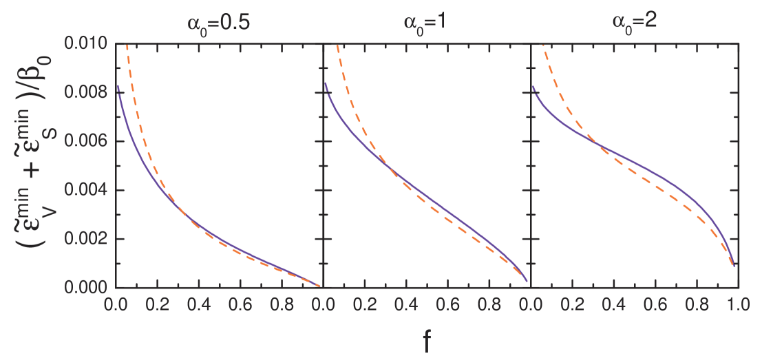
Figure 8: Comparison of the effective energies of droplets (solid curves) and slabs (dashed curves) in the Coulomb limit (for $\beta_{1}=10^{-3}$).

References

- [1] A. B. Migdal, Rev. Mod. Phys. 50 (1978) 107.
- [2] A. B. Migdal, E. E. Saperstein, M. A. Troitsky and D.N. Voskresensky, Phys. Rep. 192 (1990) 179.
- [3] V. Thorsson, M. Prakash and J.M. Lattimer, Nucl. Phys. A572 (1994) 634.
- [4] T. Tatsumi, Prog. Theor. Phys. Suppl, 120 (1995) 111.
- [5] N.K. Glendenning, Phys. Rev. D46 (1992) 1274.
- [6] S. Reddy, G.F. Bertsch and M. Prakash, Phys. Lett. B475 (2000) 1.
- [7] D. Blaschke, H. Grigorian and G. Pogosian, astro-ph/0008005.
- [8] N.K. Glendenning, Phys. Rep. 342 (2001) 393.
- [9] N.K. Glendenning and J. Schaffner-Bielich, Phys. Rev. C60 (1999) 025803.
- [10] M. Christiansen and N.K. Glendenning, astro-ph/0008207.
- [11] M. Christiansen, N.K. Glendenning and J. Schaffner-Bielich, Phys. Rev. C62 (2000) 025804.
- [12] J.A. Pons, S. Reddy, P.J. Ellis, M. Prakash and J.M. Lattimer, Phys.Rev., C62 (2000) 035803.
- [13] M. Yasuhira and T. Tatsumi, Nucl. Phys. A690 (2001) 769.
- [14] M. Alford, K. Rajagopal, S. Reddy and F. Wilczek, Phys.Rev. D64 (2001) 074017.
- [15] T. Norsen and S. Reddy, Phys.Rev. C63 (2001) 065804.
- [16] D.G. Ravenhall, C.J. Pethick and J.R. Wilson, Phys. Rev. Lett. 50 (1983) 2066.
- [17] H. Heiselberg, C.J. Pethick and E.F. Staubo, Phys. Rev. Lett. 70 (1993) 1355.
- [18] A.B. Migdal, V.S. Popov, and D.N. Voskresensky, JETP 45 (1977) 436.
- [19] D.N. Voskresensky, G.A. Sorokin and A.I. Chernoutsan, JETP Lett. 26 (1977) 465.
- [20] D.N. Voskresensky, and A.I. Chernoutsan, Sov. J. Nucl. Phys. 27 (1978) 742.
- [21] D.N. Voskresensky, M. Yasuhira and T. Tatsumi, Phys. Lett. B541 (2002) 93.
- [22] K.Rajagopal, F. Wilczek, hep-ph/0011333; T. Schäfer and E. Shuryak, Lect. Notes Phys. 578 (2001) 203; P.F. Bedaque and T. Schäfer, Nucl.Phys. A697 (2002) 802.
- [23] K. Iida, G. Baym, Phys. Rev. D66 (2002) 014015.
- [24] T. Tatsumi and M. Yasuhira, Nucl. Phys. A670 (2000) 218.
- [25] E.M. Lifshitz and L.P. Pitaevsky, Statistical Physics, part I, Pergamon press 1980.
- [26] R.G. Parr and W. Yang, Density-Functional Theory of Atoms and Molecules, (Oxford U. Press, 1989).
- [27] G. Baym, H.A. Bethe and C.J. Pethick, Nucl. Phys. A175 (1971) 225.
- [28] H. Heiselberg and M. Hjorth-Jensen, Phys. Rep. 328 (2000) 237.
- [29] N.K. Glendenning and S. Pei, Phys. Rev. C52 (1995) 2250.
- [30] R. Tamagaki and T. Tatsumi, Prog. Theor. Phys. Supl. 112 (1993) 277.
- [31] M.S. Berger and R.L. Jaffe, Phys. Rev. C35 (1987) 213; Phys. Rev. C44 (1991) R566.
- [32] B.D. Serot and J.D. Walecka, Adv. Nucl. Phys, 16 (1986) 1.
=0.9
=0.82
=0.99
=0.82
=0.99
=
0.99
=0.99
=0.99