A study of randomness, correlations and collectivity in the nuclear shell model

Abstract

A variable combination of realistic and random two-body interactions allows the study of collective properties, such as the energy spectra and B(E2) transition strengths in ⁴⁴Ti, ⁴⁸Cr and ²⁴Mg. It is found that the average energies of the yrast band states maintain the ordering for any degree of randomness, but the B(E2) values lose their quadrupole collectivity when randomness dominates the Hamiltonian. The high probability of the yrast band to be ordered in the presence of pure random forces exhibits the strong correlations between the different members of the band.

I Introduction

Nuclei display very regular spectral patterns. Low energy states in medium- and heavy-mass even-even nuclei allow their classification in terms of seniority, anharmonic vibrator and rotor nuclei zamfi94 , according to the ratio of the excitation energies of the states $4_{1}$ and $2_{1}$. While this regular behavior has been usually related with specific forces, the investigation of the energy spectra with random interactions joh98 ; joh99 has shown that many body states are strongly correlated even in the presence of random two-body interactions. Random interactions in bosonic Hilbert spaces, like those used in the IBM and the vibron model, exhibit a large predominance of vibrational and rotational spectra, strongly suggesting that in boson spaces collectivity is an intrinsic property of the space of nuclear states bij00 ; BF00_1 ; BF00_2 . Recently several studies were performed with random (tbre) and displaced random ensembles in order to simulate realistic systems hor01 ; vz02 , in particular to investigate the dominance of $0+$ states zhao02_2 ; zhao02_3

In the nuclear shell model the transition between random and collective behavior in the energy spectra of ²⁰Ne generated by two-body forces was addressed in cor82 . Collectivity was generated with a quadrupole-quadrupole force, while a residual random interaction was included in the Hamiltonian in order to study its consequences on the system’s spectroscopic properties. Both the eigenvalue distribution and the overlap between the SU(3) and calculated wave functions exhibit the smooth path from a Hamiltonian dominated by the collective force to a random, non-collective, one.

The present work aims to extend these ideas by studying the transition from a realistic parametrization of the two-body force to a purely random one, in complex systems like ²⁴Mg, ⁴⁴Ti and ⁴⁸Cr. The realistic interactions we have chosen are the universal Wildenthal Wil interaction for the sd-shell, and the KB3 kb3 for the fp-shell. The probability for each state in the yrast band to follow a sequence where the higher energies correspond to the states with the larger angular momentum is studied by varying the mixing between realistic and random forces in the Hamiltonian. The evolution of the average energies for each member of the band, as well as its B(E2) values, is also reported.

II Band structure

The combination of random and realistic interactions is taken as  cor82

$$H=aH_{C}+bH_{R}\hbox{,~{}~{}~{}with~{}~{}~{}}a+b=1,$$ (1)

where $H_{C}$ is a realistic Hamiltonian and $H_{R}$ is a two body random ensemble. Both $H_{C}$ and $H_{R}$ are written as DZ

$$H=\sum_{r\leq s,t\leq u}V_{rstu}^{JT}Z^{\dagger}_{rs,JT}\cdot Z_{tu,JT}~{},$$ (2)

in terms of scalar products of the normalized pair creation operators $Z^{\dagger}_{ij,JT}$ and its Hermitian conjugate $Z_{kl,JT}$, where $r,s,\ldots$ specify sub-shells associated with individual orbits, and $J,T$ the coupled angular momentum and isospin. For the realistic Hamiltonian $V_{rstu}^{JT}$ is the Wildenthal or $KB3$ interaction. For the random case the $V_{rstu}^{JT}$ matrix elements are taken from a two body random ensemble (TBRE), i.e., to be real and normally distributed with mean zero and width $\sigma$ for the off-diagonals and $\sqrt{2}\sigma$ for the diagonals. The values of the width $\sigma$ are taken from the realistic interactions: 1.34 MeV and 0.60 MeV, for the sd- and fp-shells, respectively. The parameter $b$ is varied from 0 to 1, to cover the different mixing from the realistic interaction to a pure random force.

II.1 The fp shell

As a first example we take ⁴⁸Cr, a rotational nucleus which has been widely studied in full shell model calculations. In the present case the diagonalization is performed in the $f_{\frac{7}{2}}p_{\frac{3}{2}}$ shell with the code Antoine cau89 , using a KB3 interaction pz90 without single particle energies. Fig. 1 shows the average energies $\overline{E_{J}}$ of the lowest energy state for each angular momentum J= 0, 2, …, 16 $\hbar$, the yrast band, calculated for 960 samples of the random interaction.

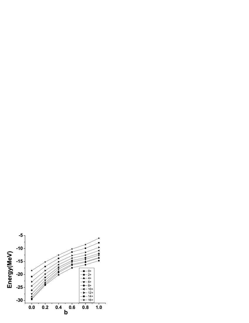
Figure 1: Average energy of 960 runs for each angular momentum of the ground band in ⁴⁸Cr.

The vertical axis displays the average energy of each state, as a function of the mixing parameter $b$. At the left hand side the realistic energies are shown, with its distinctive rotor pattern. As $b$ increases to the right, the order between the different members of the bands is maintained, but their relative separation changes. The average energies in the right hand side, the pure random Hamiltonian, still exhibit a band structure but have lost their quadrupole collectivity, as discussed below in connection with their B(E2) values.

The evolution of the average ground state band of ⁴⁴Ti, calculated in the full pf-shell, is shown in Fig. 2 as a function of the mixing parameter $b$. It can be seen that the relative ordering of the states with different angular momentum is maintained, but their relative separations vary significantly in the transition from the realistic to the random Hamiltonian. However, up to $b=0.6$ the change is mostly a scale variation, with the nearly equidistant structure of the band keeping its form. The energy spectra evolves from a vibrational equidistant form at $b=0$ to a mixed, yet ordered, spectrum for pure random forces. The average ground state energy increases with the mixing to a maximum value, with a slight decrease for $b=1$.

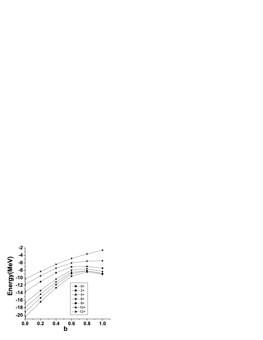
Figure 2: Average energy of 960 runs for each angular momentum of the ground band in ⁴⁴Ti.

Similar patterns of evolution of the energy centroids for each angular momentum, as function of the mixing parameter, were found in several other nuclei like ^46,48Ca and ⁴⁶Ti. While for ⁴⁶Ti, the centroid of the J=2 state is lower in energy than the J=0 state for a pure random Hamiltonian, in general for these nuclei and others in the sd-shell the average energy ordering is conserved, and there is a gradual change in the energy spectra.

The width $\sigma$ associated with the lowest average energy for each angular momentum, calculated as the square root of the variance, is shown in Fig. 3 for the gs-band of ⁴⁸Cr, as a function of the angular momentum, for different values of the mixing parameter $b$. The energy width increases with the mixing, from 1.5 MeV for $b=0.2$ to 7-9 MeV for $b=1.0$. Given that, as $b$ increases, these widths become larger than the gaps between the average energies, they indicate a strong mixing between different bands, an effect closely associated with the lack of collectivity discussed bellow. As a function of the angular momentum all the widths are essentially flat, showing a moderate increase for the largest angular momenta.

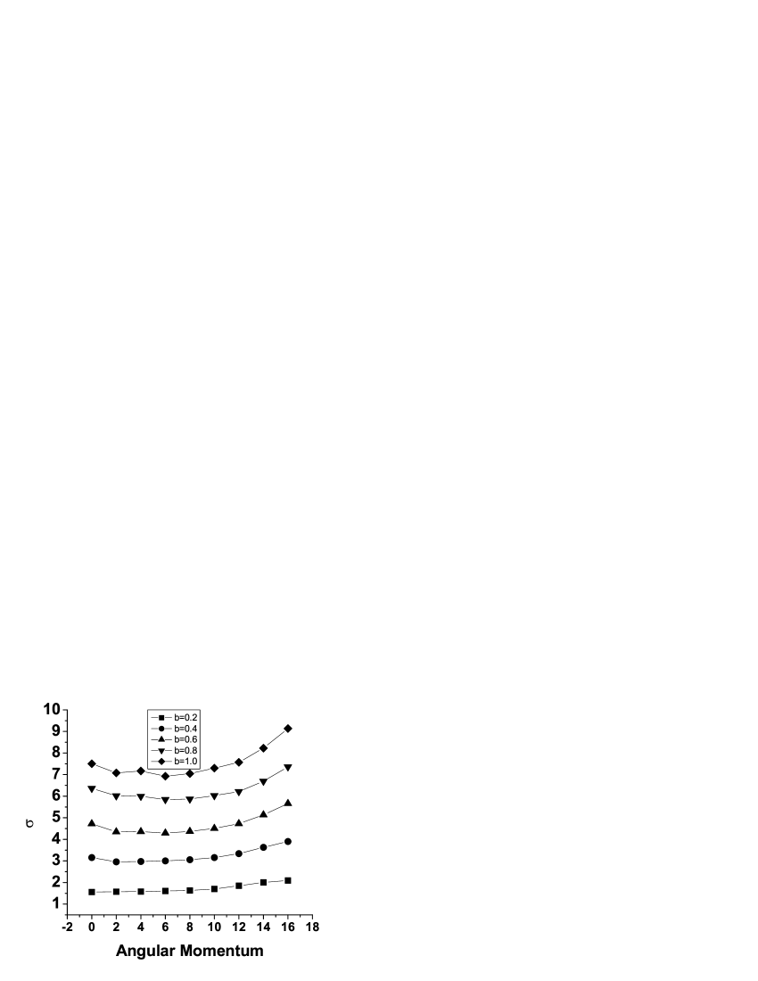
Figure 3: Average energy width of 960 runs for each angular momentum of the ground band in ⁴⁸Cr.

The energy widths are larger than the relative energy differences between adjacent states in the g.s. band, implying that there are individual cases in which the spectrum is not ordered. However, the number of runs with a completely ordered spectrum is large even for pure random interactions, as is discussed in detail bellow.

II.2 The sd-shell

Calculations in the sd-shell can be done for the full shell and an arbitrary number of active particles. The realistic interaction used in this case is the universal Wildenthal interaction (USD Wil ). The nucleus ²⁴Mg offers a rich enough system, where three bands can be studied simultaneously. They correspond, for $b=0$, to the ground state (gs), $\beta$- and $\gamma$- bands. The first two start with J=0 and contain only even-J states, while the $\gamma$- band starts with J = 2 and includes states with both even and odd angular momenta, up to J = 8. Following the evolution of the average energy levels as the mixing parameter $b$ increases, we reconstruct the three bands for each value of $b$. Nevertheless, for a pure random interaction one can show that the states have lost their quadrupole collectivity (see bellow), and for this reason they do not form bands in the usual sense.

In Fig. 4 the average energies for each angular momentum, for the ground, $\beta$- and $\gamma$- bands in ²⁴Mg, are presented for different values of the mixing parameter $b$.

Figure 4: Average energy of 960 runs for each angular momentum of three bands in ${}^{24}Mg$, see text for labels description.

The most relevant features observed in Fig. 4 are that the three bands evolve in a similar way, keeping their internal order as well as the relative separation between the bands. The correlation between increasing energy and angular momentum is strictly followed in all the averaged bands. The absolute ground state energy becomes larger as the mixing parameter increases, following the same pattern found in the fp-shell.

III Ordering probabilities

In order to further study these systems, we have analyzed the probability that each state in the band has the usual ordering i.e, the largest the angular momentum, the highest the energy for a given band. To do so we counted the number of runs where the first J=0 state is the ground state, or the first excited state in the band, the second excited state, and so on, in the 960 runs. We did the same for the states with angular momenta J = 2, 4, … In Table I the percentages for ⁴⁸Cr with a mixing of $b=0.4$ are listed. All the states have a probability of at least 90% to occupy its physically expected place, while the dispersion is very small.

$J+$	1st	2nd	3rd	4th	5th	6th	7th	8th	9th
$0$	96.56	1.04	1.25	0.52	0.42	0.10	0.00	0.10	0.00
$2$	1.56	91.88	5.31	0.62	0.21	0.21	0.10	0.00	0.10
$4$	0.21	5.62	92.29	1.04	0.42	0.21	0.21	0.00	0.00
$6$	0.52	0.94	0.42	92.50	4.27	0.94	0.21	0.00	0.21
$8$	0.73	0.21	0.21	3.75	93.02	1.04	0.31	0.52	0.21
$10$	0.00	0.00	0.10	0.83	0.52	95.21	2.29	0.83	0.21
$12$	0.00	0.00	0.21	0.62	0.83	2.08	96.04	0.21	0.00
$14$	0.21	0.21	0.10	0.10	0.31	0.10	0.52	97.40	1.04
$16$	0.21	0.10	0.10	0.00	0.00	0.10	0.31	0.94	98.23

Table 1: Probability for each angular momentum state to be in the correct position in the ground state band with $b=0.4$ for ⁴⁸Cr.

Table II lists the probability for states of each angular momentum in ⁴⁸Cr to occupy the indicated place for a purely random Hamiltonian, i.e. $b=1$. The probabilities of being in its expected place run from 44% for J = 2 to 83% for J = 16. States with J = 0, 2 and 4 are those which more often fail to occupy their place, as they tend to exchange positions. These results represent an extension of previous studies concerning the probability of each state to be the ground state, listed in the first column Zhao01 .

$J+$	1st	2nd	3rd	4th	5th	6th	7th	8th	9th
$0$	60.31	8.85	9.27	4.48	4.90	2.50	1.98	2.29	5.42
$2$	17.40	43.54	16.98	4.17	3.96	2.60	3.12	5.00	3.23
$4$	6.56	27.71	47.08	6.46	2.40	2.71	4.38	2.19	0.52
$6$	2.40	5.42	9.79	64.58	6.25	5.31	3.12	1.77	1.35
$8$	3.12	3.65	4.69	9.06	69.58	6.46	1.15	1.56	0.73
$10$	1.35	2.50	3.44	5.94	7.19	74.69	3.54	0.62	0.73
$12$	1.98	1.88	5.52	2.50	3.23	3.65	79.06	1.98	0.21
$14$	1.15	5.62	1.98	1.67	0.94	1.25	2.40	80.10	4.90
$16$	5.73	0.83	1.25	1.15	1.56	0.83	1.25	4.48	82.92

Table 2: Probability for each angular momentum state to be in different positions, for the ⁴⁸Cr ground state band with $b=1.0$.

Table III displays the probability for each angular momentum state to be in a given position, in the ⁴⁴Ti ground state band with $b=1.0$. These probabilities have values between 44% for J=2 to 95% for J = 12. The fact that the states with J=2 and 4 have less than 50% probability of occupying in their places is strongly connected with the closeness of their average energies, shown in Fig. 2 for $b=1$.

$J+$	1st	2nd	3rd	4th	5th	6th	7th
$0$	46.25	19.27	20.42	6.98	5.62	1.35	0.10
$2$	16.56	39.90	24.38	11.56	5.83	1.25	0.52
$4$	21.04	25.83	40.10	9.38	3.02	0.21	0.42
$6$	8.44	10.42	10.10	64.58	5.42	1.04	0.00
$8$	6.56	3.96	4.27	5.83	76.77	2.08	0.52
$10$	0.10	0.52	0.52	1.25	2.60	92.08	2.92
$12$	1.04	0.10	0.21	0.42	0.73	1.98	95.52

Table 3: Probability for each angular momentum to be in different positions, for the ⁴⁴Ti ground state band, with $b=1.0$.

Tables IV, V and VI display the probability that states with different angular momenta in ²⁴Mg have to occupy a given place in each band for $b=1.0$, for the ground state, $\beta$- and $\gamma$- band, respectively. In most cases the diagonal probability, i.e. the probability that each state occupies its expected place, is larger than 50%. The exceptions are the states with J = 2 and 3 in the $\gamma$-band, and those with J= 0 and 2 in the $\beta$-band, whose probabilities lie between 38% and 48%.

$J+$	1st	2nd	3rd	4th	5th
$0$	56.56	12.40	12.29	6.77	11.98
$2$	18.12	52.81	13.12	9.79	6.15
$4$	9.06	19.58	63.85	5.52	1.98
$6$	4.38	11.25	6.98	71.25	6.15
$8$	11.88	3.96	3.75	6.67	73.75

Table 4: Probability for states belonging to the ground state band in ²⁴Mg, with $b=1.0$, to occupy different positions.

$J+$	1st	2nd	3rd	4th	5th	6th	7th
$2$	45.21	22.92	7.50	5.94	4.79	6.46	7.19
$3$	27.40	38.33	13.54	6.15	4.17	6.04	4.38
$4$	7.40	14.90	50.62	15.94	7.29	3.02	0.83
$5$	7.71	12.08	15.10	58.85	5.00	1.04	0.21
$6$	3.44	3.75	6.25	7.60	66.25	11.88	0.83
$7$	5.10	4.27	4.17	3.96	10.83	64.38	7.29
$8$	3.75	3.75	2.81	1.56	1.67	7.19	79.27

Table 5: The same as in Table 4, for the $\gamma$-band.

$J+$	1st	2nd	3rd	4th	5th
$0$	46.67	20.73	13.54	8.44	10.62
$2$	28.02	47.40	12.81	8.44	3.33
$4$	13.23	19.27	65.62	1.88	0.00
$6$	6.35	9.38	5.94	77.50	0.00
$8$	5.73	3.23	2.08	3.75	85.21

Table 6: The same as in Table 4, for the $\beta$-band.

IV Collectivity

A sensitive measure of the quadrupole collectivity of the system is the B(E2,$2_{1}\rightarrow 0_{gs}$) transition strength. The distribution of B(E2) strengths in ⁴⁸Cr, for four different values of the mixing parameter $b$, is shown in Fig. 5. Its experimental value is 230 $e^{2}b^{2}$. For $b=0.2$, shown in insert a), the distribution is concentrated around the experimental B(E2) value. For $b=0.4$, insert b), the increase in the random components of the Hamiltonian leads to an important fragmentation of the B(E2) intensity with four clusters, one near zero, the second one around 75 $e^{2}b^{2}$, the next one near 170 $e^{2}b^{2}$ and the last one close to the measured value. For $b=0.6$, insert c), most of the B(E2) values are very small, with some intensity at the collective B(E2) values. Finally, in insert d) the distribution of B(E2) values for a purely random Hamiltonian is shown. It is strongly concentrated at very small values, showing a complete lack of quadrupole collectivity, in consonance with the findings of Ref. cor82 .

Figure 5: Probability densities for B(E2,$2\rightarrow$ 0) for ⁴⁸Cr.

Fig. 6 displays the distribution of B(E2,$2\rightarrow$ 0) values for ⁴⁴Ti. Insert a) shows the results for $b=0.2$, with a narrow distribution around the measured value of 147 $e^{2}b^{2}$. In insert b) the distribution for $b=0.4$ is presented, which is concentrated around the same value. For $b=0.6$, Fig. 5 c), the distribution is still concentrated around the collective B(E2) values despite the dominance of the random component in the Hamiltonian. However, this collectivity is completely lost when pure random forces are employed, as shown in Fig. 5 d).

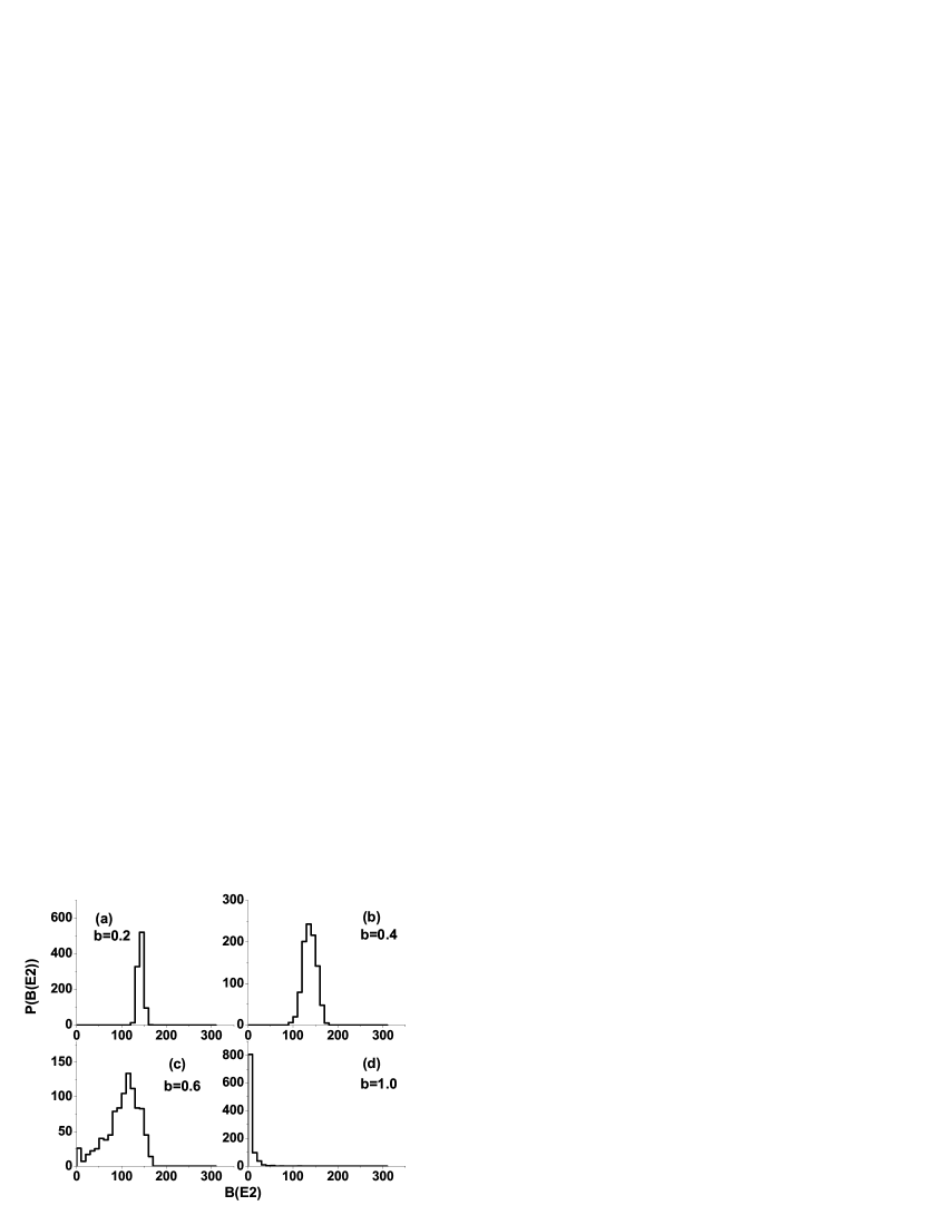
Figure 6: Probability density for B(E2,$2\rightarrow$ 0)for ⁴⁴Ti.

A useful indicator of collectivity is the energy ratio

$$R={\frac{E_{4^{+}_{1}}}{E_{2^{+}_{1}}}}.$$ (3)

The value R = 2 is associated with a harmonic oscillator spectrum, while R = 3.3 characterizes a rigid rotor structure.

Fig. 7 shows the distribution of energy ratios for ⁴⁸Cr. The case $b=0.2$, shown in insert a), does exhibit the actual rotor behavior of this nucleus. This feature remains dominant for $b=0.4$, insert b), while for $b=0.6$ the distribution of energy ratios is wide and peaked at R=1. For $b=1.0$, shown in Fig 7 d), the distribution is very wide, with a clear dominance of the R=1 ratio, in correspondence with the near degeneracy of the states with J= 2 and 4 for $b=1$, as shown in Fig. 1.

Figure 7: Probability densities for the energy ratios R for ⁴⁸Cr.

⁴⁴Ti has a structure closer to a harmonic oscillator than to a rotor. This feature can be seen in Fig. 8 a), which displays the distribution of energy ratios for $b=0.2$, narrowly concentrated around R = 2. For $b=0.4$ and $0.6$, inserts b) and c), the vibrational structure is wider but well defined. For a pure random interaction, Fig. 8 d), the distribution is peeked at R = 1, reflecting the near degeneracy of the average energies $\bar{E}_{2}$ and $\bar{E}_{4}$. The displacement of the most probable energy ratio R to 1 is accompanied by a lack of quadrupole coherence, in consistent with the previous analysis of the B(E2) transition strengths.

Figure 8: Probability densities for energy ratios R for ⁴⁴Ti.

V Correlation and coherence.

Having discussed the evolution of the energy centroids as a function of the mixing parameter $b$, and the probability for each state to occupy a certain position in the band, it is natural to study the probability that the ground state band has all its states properly ordered. This probability, given as the percentage of results from the 960 runs which are properly ordered, is shown in Fig. 9 for ⁴⁸Cr, ⁴⁴Ti and ²⁴Mg. In the three cases it is apparent that the spectrum is always ordered when the realistic interaction dominates the Hamiltonian, and that the probability for the ground state band to be ordered decreases to about 35% for a fully random Hamiltonian.

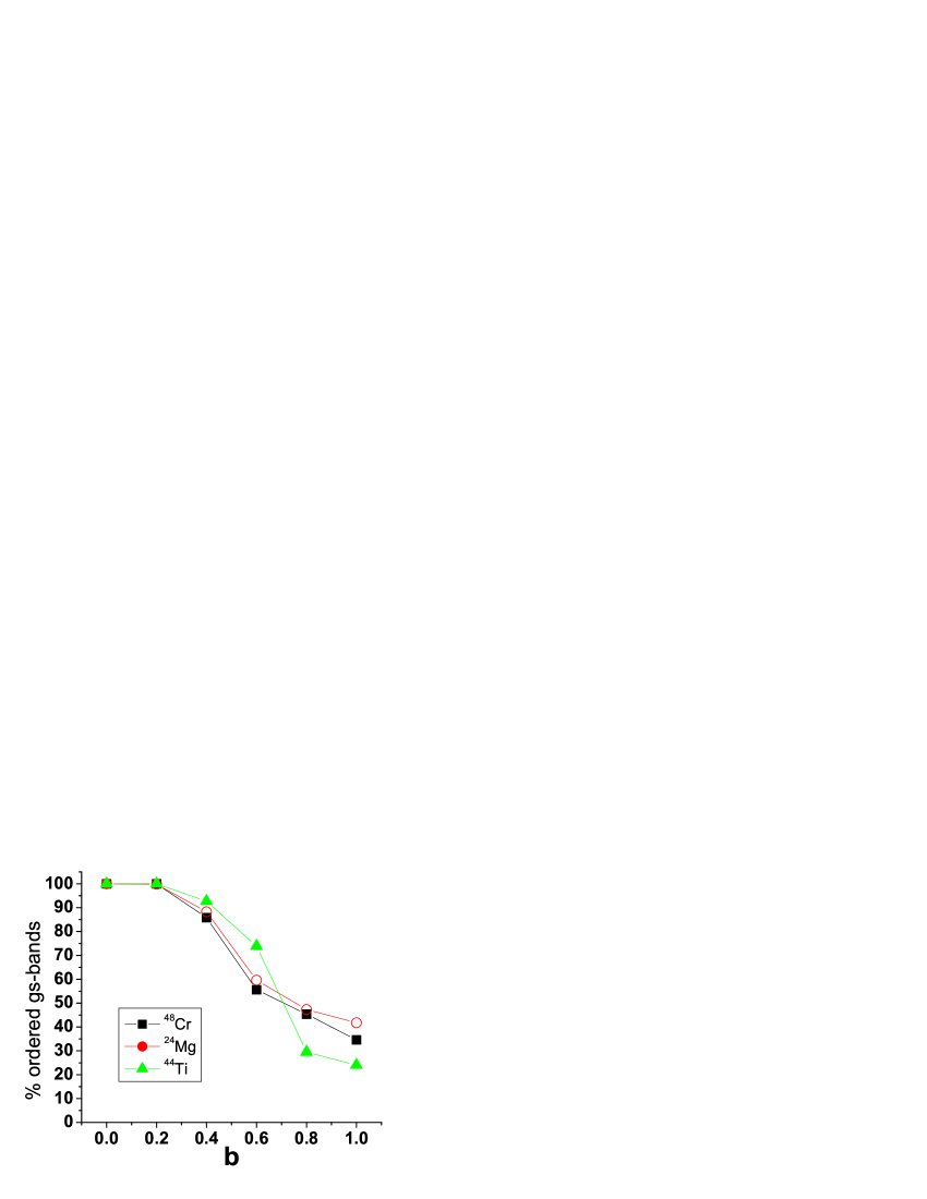
Figure 9: Percentage of ordered bands vs $b$ for Cr,Ti and Mg.

It is worth emphasizing that if these probabilities were independent of each other, the probability to find a completely order band would be the product of the probabilities for each state, i.e., the product of the diagonal elements of the matrices shown in Tables II, III and IV. However, these products are all smaller than 0.04, far smaller than the probabilities of 25 - 45 % found in these calculations. These results show that the many body states obtained with two-body random forces are strongly correlated. This correlation in their energies is not, however, associated with quadrupole coherence, which is lost for pure random forces cor82 . The subtle connection between correlation and coherence requires further analysis.

The correlation $r$ for each value of the mixing parameter $b$, between the states with energies $E_{J}$ and $E_{J+2}$ in the sample, can be quantitatively calculated as DP

$$r={\frac{cov(E_{J},E_{J+2})}{\sigma_{E_{J}}\sigma_{E_{J+2}}}}$$ (4)

where

$$cov(E_{J},E_{J+2})=\frac{\sum_{i}^{n}({E_{J}}_{i}-{\overline{E_{J}}})({E_{(J+2)}}_{i}-{\overline{E_{J+2}}})}{n}$$ (5)

Here, ${cov(E_{J},E_{J+2})}$ is the covariance of the two distributions, $\sigma$ is the square root of the variance $cov(E_{J},E_{J})$, and $n$ is the size of the space. If $r=1$ the distributions are fully correlated, while if $r\approx 0$ there is no correlation between them. In table VII the correlation $r$ for pairs of energies in the ground state band of ⁴⁸Cr are listed .

$J,J+2$	0.2	0.4	0.6	0.8	1.0
$0+,2+$	0.966	0.928	0.937	0.949	0.991
$2+,4+$	0.996	0.991	0.991	0.991	0.986
$4+,6+$	0.992	0.977	0.974	0.981	0.980
$6+,8+$	0.991	0.989	0.992	0.993	0.993
$8+,10+$	0.987	0.989	0.989	0.989	0.987
$10+,12+$	0.985	0.982	0.982	0.984	0.985
$12+,14+$	0.992	0.989	0.987	0.986	0.986
$14+,16+$	0.992	0.992	0.990	0.989	0.988

Table 7: Correlations $r$ between neighbor states in ${48}Cr$.

The presence of strong correlations between the different wave functions obtained with two-body random forces, suggests that the many-body states could be well approximated by a small number of configurations which may correspond to definite shapes, as was found for bosonic models. This would imply that the very large number of shell-model many-body states would be limited or constrained by the geometry imposed by the existence of a two-body Hamiltonian, even for the case that its components are randomly selected chau .

VI The DTBRE case

In vz02 it was shown that a displaced two body random ensemble (DTBRE) gives rise to coherent rotor patterns. To complement the present study we analyze in this section the transition from the realistic KB3 interaction to a DTBRE in the ground state band of ⁴⁸Cr. The DTBRE correspond to matrix elements with a normal distribution centered at $c=-1.0$ and width $\sigma=0.6$. Fig. 10 shows the evolution of the average energies in the ground-state band of ⁴⁸Cr as a function of the mixing parameter $b$.

Figure 10: Average energy of 960 runs for each angular momentum of the ground band in ⁴⁸Cr with a DTBRE mixing.

At variance from the results shown in Fig. 1, 2 and 4, when the random component of the interaction increases the absolute energies continuously decrease. As expected, the rotor structure survives the transition from realistic to random interactions with nearly no changes.

In Table VIII we show the probability for states belonging to the ground state band in ⁴⁸Cr, to occupy its expected place. Notice that even for $b=1.0$, when the pure displaced random ensemble is employed, the probability for each state to be in its place is larger than $88\%$, thus exhibiting a high ordering. The percentage of fully ordered bands for each mixing is equally large: 100% for $b=0.2$, 89% for $b=0.6$ and 70% for $b=1.0$. If the centroid of the DTBRE is displaced to more negative values, like $c=-3.0$, 100 % of the bands are ordered vz02 . The distribution of B(E2) probabilities exhibits a clear presence of quadrupole coherence for $c=-1$. They are concentrated in a narrow peak around the collective B(E2) values for $c=-3$ vz02 .

$J+$	$b=0.2$	$0.4$	$0.6$	$0.8$	$1.0$
$0$	99.58	99.79	97.71	92.08	88.12
$2$	98.75	99.27	95.00	86.04	80.31
$4$	98.96	99.38	95.21	86.46	79.90
$6$	99.27	99.58	96.35	91.46	87.50
$8$	99.27	99.69	98.02	94.69	91.15
$10$	99.58	99.90	98.96	96.77	94.38
$12$	99.69	99.90	98.65	96.77	95.00
$14$	99.58	99.58	94.79	90.62	87.92
$16$	99.58	99.69	95.00	90.42	88.33

Table 8: Probabilities for states belonging to the ground state band in ⁴⁸Cr, to occupy their ordered place, for a DTBRE mixing.

VII Summary and conclusions

The average energies of states with different angular momentum preserve their ordering inside the band when the Hamiltonian is changed smoothly from a realistic to a random one. Ground state energies increase as a function of the mixing parameter. The quadrupole collectivity is lost when the Hamiltonian is dominated by random two-body forces, and the probability that the ground state band remains ordered diminishes to 25-45% in the random limit, which is anyway far larger than the product of the probabilities for each state to be in its place, thus exhibiting the strong correlations between the different wave functions. On the other hand, when displaced two-body random ensembles are employed, the average energies decrease as the random component increases, and the rotor pattern remains unchanged.

- (1) N. V. Zamfir, R. F. Casten, and D. S. Brener, Phys. Rev. Lett. 72, 3480 (1994).
- (2) C. W. Johnson, G. F. Bertsch, and D. J. Dean, Phys. Rev. Lett. 80, 2749 (1998).
- (3) C. W. Johnson, G. F. Bertsch, D. J. Dean, and I. Talmi Phys. Rev. C 61, 014311 (1999)
- (4) R. Bijker,A. Frank, and S. Pittel Phys. Rev. C 60, 021302 (1999).
- (5) R. Bijker, and A. Frank, Phys. Rev. Lett. 84, 420 (2000)
- (6) R. Bijker, and A. Frank, Phys. Rev. C 62, 014303 (2000)
- (7) M. Horoi, B. A. Brown, V. Zelevinsky, Phys. Rev. Lett. 87, 062501(2001).
- (8) V. Velázquez and A. P. Zuker, Phys. Rev. Lett. 88, 072502 (2002).
- (9) Y. M.Zhao, A.Arima, and Y.Yoshinaga, arXiv:nucl-th/0206040.
- (10) Y. M.Zhao, A.Arima, and Y.Yoshinaga, arXiv:nucl-th/0206041.
- (11) P. Chau, A. Frank, N. Smirnova and P. Van Isacher, to be published.
- (12) A. Cortes, R. U. Haq, and A. P. Zuker, Phys. Lett. B 115, 1 (1982).
- (13) B.H. Wildenthal, Prog. Part. Nucl. Phys. 11, 5 (1984).
- (14) T.T.S. Kuo and G.E. Brown, Nucl. Phys. A 114, 235( 1968); A. Poves and A.P. Zuker, Phys Rep.70, 235 (1981).
- (15) M. Dufour and A.P. Zuker, Phys. Rev.C 54, 1641 (1996).
- (16) E. Caurier, computer code antoine, CRN, Strasbourg (1989).
- (17) A. Poves and A. P. Zuker, Phys. Rep. 70 (1990) 235.
- (18) Y. M. Zhao, A. Arima, and Y. Yoshinaga, arXiv:nucl-th/0112075.
- (19) D. Peña Sánchez; Estadística modelos y métodos, Ed. Alianza Universidad Textos (1986).