Low Energy Pion–Nucleon Scattering in the Heavy Baryon and Infrared Schemes

Abstract

We study pion–nucleon scattering with a chiral Lagrangian of pions, nucleons, and $\Delta$-isobars to order $Q^{3}$, where $Q$ is a generic small momentum. We compare the results from heavy baryon chiral perturbation theory with those from the infrared regularization scheme. While the former provides a reasonable fit to the data out to a pion c.m. kinetic energy of 100 MeV, the latter is only able to fit up to 40 MeV and even then the parameters obtained are unreasonable. Difficulties with the infrared scheme in the $u$-channel are discussed.

I Introduction

Pion-nucleon scattering is a fundamental process that one would like to describe using the low-energy realization of quantum chromodynamics, namely chiral perturbation theory [1, 2]. This is an attractive approach because it not only embodies chiral symmetry, which is fundamental to low-energy physics, but also offers a systematic expansion in powers of the momentum. Further it ensures unitarity order by order. Gasser and Leutwyler [2] have shown that chiral perturbation theory works nicely for mesons and high accuracy can now be achieved for the $\pi\pi$ scattering lengths [3].

However, the power counting fails when baryons are introduced [4]. The power counting can be restored in heavy baryon chiral perturbation theory (henceforth referred to as HB) [5] where the heavy components of the baryon fields are integrated out. An alternative – the infrared regularization scheme (henceforth referred to as IR) – has been proposed [6], based on the ideas in Ref. [7]. This preserves the chiral power counting and has the advantage that it is manifestly Lorentz invariant and avoids the voluminous effective Lagrangian of the HB approach. Generally favorable results have been obtained with the IR scheme in a number of applications [8]. By suitable approximation of the IR expressions the HB formulae can be regained. A recent review of the HB and IR formalisms has been given by Meißner [9].

The first fit to the pion-nucleon scattering phase shift data using chiral perturbation theory was carried out in Ref. [7], henceforth referred to as I, using the HB scheme. In addition to the nucleon and pion fields, the $\Delta$ resonance field was included explicitly since the intent was to fit out to energies in the $\Delta$ resonance region. The calculation was carried to ${\cal O}(Q^{3})$, where $Q$ is a generic small momentum scale, and it was found possible to obtain a reasonable fit up to energies slightly below the $\Delta$ resonance. Subsequently Fettes and Meißner carried out several HB studies both with [10] and without [11, 12] explicit inclusion of the $\Delta$ field. The calculation with the $\Delta$ field to ${\cal O}(Q^{3})$ appeared to be a little better than the ${\cal O}(Q^{4})$ calculation without it; for further discussion see Ref. [13]. Fettes and Meißner [14] have also studied isospin violation in the $\pi-N$ system, although here we shall focus on the isospin symmetric case. All of these calculations were carried out with the HB approach and it is natural to examine the IR method in this context. Becher and Leutwyler [15] have used the IR approach in the sub-threshold region, where the HB scheme is inappropriate, and found that the IR representation of the scattering amplitude was not sufficiently accurate to allow the extrapolation of the experimental data to this region. The purpose of the present work is to study the IR scheme in the physical region at ${\cal O}(Q^{3})$ and compare it with the HB approach in order to see whether an improved fit to the phase shift data can be obtained.

The organization of this paper is as follows. In Sec. II we review our notation for the effective Lagrangian and discuss the ${\cal O}(Q^{3})$ calculation of the scattering amplitudes in the IR scheme and their reduction to HB form. Formulae for the $\sigma$ term and effective vertex couplings are also given. In Sec. III our fit to the phase shift data is described, first for the HB scheme and then for the IR approach. Our conclusions are presented in Sec. IV. Expressions for the IR integrals mentioned in the text are given in the Appendix, together with their HB reductions.

II Formalism

A Effective Lagrangian

In the IR or HB schemes the Feynman diagrams for $\pi N$ scattering follow Weinberg’s power counting rule [16]. Define

$$\nu=1+2L+\sum_{i}V_{i}\Big{(}d_{i}+\frac{1}{2}n_{i}-2\Big{)}\ ,$$ (1)

where $L$ is the number of loops, $V_{i}$ is the number of vertices of type $i$ characterized by $n_{i}$ baryon fields and $d_{i}$ pion derivatives or pion mass factors. Then a given diagram is of leading order $Q^{\nu}$, where $Q$ is a small or “soft” momentum scale, for example, the pion mass $m$, the pion momentum or the mass splitting between the $\Delta$-isobar and the nucleon, $\delta=M_{\Delta}-M$.

We briefly recapitulate the effective chiral Lagrangian given in I. Characterising it by $d_{i}+\frac{1}{2}n_{i}$, the order $Q^{2}$ part is

$${\cal L}_{2} = \bar{N}(i\hbox to0.0pt{/\hss}{\mkern-3.0mu{\cal D}}+g_{\rm A}\gamma^{\mu}\gamma_{5}a_{\mu}-M)N+{\textstyle{\frac{1}{4}}}f_{\pi}^{2}{\rm tr}\,(\partial_{\mu}U^{\dagger}\partial^{\mu}U)+{\textstyle{\frac{1}{4}}}m^{2}f_{\pi}^{2}{\rm tr}\,(U+U^{\dagger}-2)$$ (3)

$$+\bar{\Delta}_{\mu}^{a}\Lambda^{\mu\nu}_{ab}\Delta_{\nu}^{b}+h_{\rm A}\Big{(}\bar{\mathchoice{{\hbox{\boldmath$\displaystyle\Delta$}}}{{\hbox{\boldmath$\textstyle\Delta$}}}{{\hbox{\boldmath$\scriptstyle\Delta$}}}{{\hbox{\boldmath$\scriptscriptstyle\Delta$}}}}_{\mu}\mathchoice{{\hbox{\boldmath$\displaystyle\cdot a$}}}{{\hbox{\boldmath$\textstyle\cdot a$}}}{{\hbox{\boldmath$\scriptstyle\cdot a$}}}{{\hbox{\boldmath$\scriptscriptstyle\cdot a$}}}^{\mu}N+\bar{N}\mathchoice{{\hbox{\boldmath$\displaystyle a$}}}{{\hbox{\boldmath$\textstyle a$}}}{{\hbox{\boldmath$\scriptstyle a$}}}{{\hbox{\boldmath$\scriptscriptstyle a$}}}^{\mu}\mathchoice{{\hbox{\boldmath$\displaystyle\cdot\Delta$}}}{{\hbox{\boldmath$\textstyle\cdot\Delta$}}}{{\hbox{\boldmath$\scriptstyle\cdot\Delta$}}}{{\hbox{\boldmath$\scriptscriptstyle\cdot\Delta$}}}_{\mu}\Big{)}+\tilde{h}_{\rm A}\bar{\Delta}_{\mu}^{\,a}\gamma^{\nu}\gamma_{5}a_{\nu}\Delta^{\mu}_{a}\ ,$$

where the trace is taken over the isospin matrices. The isotriplet pion fields enter in the $SU(2)$ matrix

$$U(x)\equiv\xi^{2}=\exp(2i\pi(x)/f_{\pi})\ ,$$ (4)

where $f_{\pi}$ is the pion decay constant and $\pi(x)\equiv\mathchoice{{\hbox{\boldmath$\displaystyle\pi$}}}{{\hbox{\boldmath$\textstyle\pi$}}}{{\hbox{\boldmath$\scriptstyle\pi$}}}{{\hbox{\boldmath$\scriptscriptstyle\pi$}}}(x)\,\mathchoice{{\hbox{\boldmath$\displaystyle\cdot$}}}{{\hbox{\boldmath$\textstyle\cdot$}}}{{\hbox{\boldmath$\scriptstyle\cdot$}}}{{\hbox{\boldmath$\scriptscriptstyle\cdot$}}}\,{1\over 2}\mathchoice{{\hbox{\boldmath$\displaystyle\tau$}}}{{\hbox{\boldmath$\textstyle\tau$}}}{{\hbox{\boldmath$\scriptstyle\tau$}}}{{\hbox{\boldmath$\scriptscriptstyle\tau$}}}$, with $\textstyle\tau$ denoting the Pauli matrices. The axial vector field $a_{\mu}(x)$ and vector field $v_{\mu}(x)$ are defined by

$$a_{\mu} \equiv -{i\over 2}(\xi^{\dagger}\partial_{\mu}\xi-\xi\partial_{\mu}\xi^{\dagger})=a_{\mu}^{\dagger}={\textstyle{\frac{1}{2}}}\mathchoice{{\hbox{\boldmath$\displaystyle a$}}}{{\hbox{\boldmath$\textstyle a$}}}{{\hbox{\boldmath$\scriptstyle a$}}}{{\hbox{\boldmath$\scriptscriptstyle a$}}}_{\mu}\mathchoice{{\hbox{\boldmath$\displaystyle\cdot\tau$}}}{{\hbox{\boldmath$\textstyle\cdot\tau$}}}{{\hbox{\boldmath$\scriptstyle\cdot\tau$}}}{{\hbox{\boldmath$\scriptscriptstyle\cdot\tau$}}}={1\over f_{\pi}}\partial_{\mu}\pi-{1\over 3f_{\pi}^{3}}\pi[\pi,\partial_{\mu}\pi]+\cdots\ ,$$ (5)

$$v_{\mu} \equiv -{i\over 2}(\xi^{\dagger}\partial_{\mu}\xi+\xi\partial_{\mu}\xi^{\dagger})=v_{\mu}^{\dagger}={\textstyle{\frac{1}{2}}}\mathchoice{{\hbox{\boldmath$\displaystyle v$}}}{{\hbox{\boldmath$\textstyle v$}}}{{\hbox{\boldmath$\scriptstyle v$}}}{{\hbox{\boldmath$\scriptscriptstyle v$}}}_{\mu}\mathchoice{{\hbox{\boldmath$\displaystyle\cdot\tau$}}}{{\hbox{\boldmath$\textstyle\cdot\tau$}}}{{\hbox{\boldmath$\scriptstyle\cdot\tau$}}}{{\hbox{\boldmath$\scriptscriptstyle\cdot\tau$}}}=-{i\over 2f_{\pi}^{2}}\left(1-{\pi^{2}\over 3f_{\pi}^{2}}\right)[\pi,\partial_{\mu}\pi]+\cdots\ ,$$ (6)

both of which contain one derivative. The covariant derivative on the nucleon field ${\cal D}_{\mu}N=\partial_{\mu}N+iv_{\mu}N$. For the $\Delta$ resonance we have introduced an isovector field $\mathchoice{{\hbox{\boldmath$\displaystyle\Delta$}}}{{\hbox{\boldmath$\textstyle\Delta$}}}{{\hbox{\boldmath$\scriptstyle\Delta$}}}{{\hbox{\boldmath$\scriptscriptstyle\Delta$}}}_{\mu}=\mathchoice{{\hbox{\boldmath$\displaystyle T$}}}{{\hbox{\boldmath$\textstyle T$}}}{{\hbox{\boldmath$\scriptstyle T$}}}{{\hbox{\boldmath$\scriptscriptstyle T$}}}\Delta_{\mu}$ in terms of the standard $2\times 4$ isospin ${\textstyle{\frac{3}{2}}}$ to ${\textstyle{\frac{1}{2}}}$ transition matrix and the labels $a$ and $b$ in Eq. (3) are isospin indices. The kernel tensor in the $\Delta$ kinetic energy term is

$$\Lambda^{\mu\nu}=-(i\hbox to0.0pt{/\hss}{\mkern-3.0mu{\cal D}}-M_{\Delta})g^{\mu\nu}+i(\gamma^{\mu}{\cal D}^{\nu}+\gamma^{\nu}{\cal D}^{\mu})-\gamma^{\mu}(i\hbox to0.0pt{/\hss}{\mkern-3.0mu{\cal D}}+M_{\Delta})\gamma^{\nu}\ ,$$ (7)

suppressing isospin indices, and the covariant derivative is defined by

$${\cal D}_{\mu}\mathchoice{{\hbox{\boldmath$\displaystyle\Delta$}}}{{\hbox{\boldmath$\textstyle\Delta$}}}{{\hbox{\boldmath$\scriptstyle\Delta$}}}{{\hbox{\boldmath$\scriptscriptstyle\Delta$}}}_{\nu}=\partial_{\mu}\mathchoice{{\hbox{\boldmath$\displaystyle\Delta$}}}{{\hbox{\boldmath$\textstyle\Delta$}}}{{\hbox{\boldmath$\scriptstyle\Delta$}}}{{\hbox{\boldmath$\scriptscriptstyle\Delta$}}}_{\nu}+iv_{\mu}\mathchoice{{\hbox{\boldmath$\displaystyle\Delta$}}}{{\hbox{\boldmath$\textstyle\Delta$}}}{{\hbox{\boldmath$\scriptstyle\Delta$}}}{{\hbox{\boldmath$\scriptscriptstyle\Delta$}}}_{\nu}-\mathchoice{{\hbox{\boldmath$\displaystyle v$}}}{{\hbox{\boldmath$\textstyle v$}}}{{\hbox{\boldmath$\scriptstyle v$}}}{{\hbox{\boldmath$\scriptscriptstyle v$}}}_{\mu}\times\mathchoice{{\hbox{\boldmath$\displaystyle\Delta$}}}{{\hbox{\boldmath$\textstyle\Delta$}}}{{\hbox{\boldmath$\scriptstyle\Delta$}}}{{\hbox{\boldmath$\scriptscriptstyle\Delta$}}}_{\nu}\ .$$ (8)

We have chosen the simplest form for the $\pi N\Delta$ interaction in Eq. (3) since modifications of the type suggested by Pascalutsa [17] or modifications of the standard off-shell $Z$ parameter can be absorbed in the other parameters of the Lagrangian [18].

The order $Q^{3}$ and $Q^{4}$ parts of the Lagrangian are:

$${\cal L}_{3} = {\beta_{\pi}\over M}\bar{N}N{\rm tr}\,(\partial_{\mu}U^{\dagger}\partial^{\mu}U)-{\kappa_{\pi}\over M}\bar{N}v_{\mu\nu}\sigma^{\mu\nu}N$$ (10)

$$+{\kappa_{1}\over 2M^{2}}i\bar{N}\gamma_{\mu}\stackrel{{\scriptstyle\leftrightarrow}}{{\cal D}}_{\nu}N{\rm tr}\,(a^{\mu}a^{\nu})+{\kappa_{2}\over M}m^{2}\bar{N}N\,{\rm tr}\,(U+U^{\dagger}-2)+\cdots\ ,$$

$${\cal L}_{4} = {\lambda_{1}\over M}m^{2}\bar{N}\gamma_{5}(U-U^{\dagger})N+{\lambda_{2}\over M^{2}}\bar{N}\gamma^{\mu}D^{\nu}v_{\mu\nu}N$$ (14)

$$+{\lambda_{3}\over M^{2}}m^{2}\bar{N}\gamma_{\mu}[a^{\mu},\,U-U^{\dagger}]N+{\lambda_{4}\over 2M^{3}}i\bar{N}\sigma_{\rho\mu}\stackrel{{\scriptstyle\leftrightarrow}}{{\cal D}}_{\nu}N{\rm tr}\,(a^{\rho}D^{\mu}a^{\nu})$$

$$+{\lambda_{5}\over 16M^{4}}i\bar{N}\gamma_{\rho}\{\stackrel{{\scriptstyle\leftrightarrow}}{{\cal D}}_{\mu},\stackrel{{\scriptstyle\leftrightarrow}}{{\cal D}}_{\nu}\}\tau^{a}N\,{\rm tr}\,(\tau^{a}[D^{\rho}a^{\mu},a^{\nu}])$$

$$+{\lambda_{6}\over 2M^{2}}m^{2}\Big{\{}\bar{\mathchoice{{\hbox{\boldmath$\displaystyle\Delta$}}}{{\hbox{\boldmath$\textstyle\Delta$}}}{{\hbox{\boldmath$\scriptstyle\Delta$}}}{{\hbox{\boldmath$\scriptscriptstyle\Delta$}}}}_{\mu}\mathchoice{{\hbox{\boldmath$\displaystyle\cdot$}}}{{\hbox{\boldmath$\textstyle\cdot$}}}{{\hbox{\boldmath$\scriptstyle\cdot$}}}{{\hbox{\boldmath$\scriptscriptstyle\cdot$}}}{\rm tr}[i\partial^{\mu}(U-U^{\dagger})\mathchoice{{\hbox{\boldmath$\displaystyle\tau$}}}{{\hbox{\boldmath$\textstyle\tau$}}}{{\hbox{\boldmath$\scriptstyle\tau$}}}{{\hbox{\boldmath$\scriptscriptstyle\tau$}}}]N+\bar{N}{\rm tr}[i\partial^{\mu}(U-U^{\dagger})\mathchoice{{\hbox{\boldmath$\displaystyle\tau$}}}{{\hbox{\boldmath$\textstyle\tau$}}}{{\hbox{\boldmath$\scriptstyle\tau$}}}{{\hbox{\boldmath$\scriptscriptstyle\tau$}}}]\mathchoice{{\hbox{\boldmath$\displaystyle\cdot\Delta$}}}{{\hbox{\boldmath$\textstyle\cdot\Delta$}}}{{\hbox{\boldmath$\scriptstyle\cdot\Delta$}}}{{\hbox{\boldmath$\scriptscriptstyle\cdot\Delta$}}}_{\mu}\Big{\}}+\cdots\ .$$

Here we have used the definitions

$$\stackrel{{\scriptstyle\leftrightarrow}}{{\cal D}}_{\mu} = {\cal D}_{\mu}-(\stackrel{{\scriptstyle\leftarrow}}{{\partial}}_{\mu}-iv_{\mu})\quad;\quad v_{\mu\nu}=\partial_{\mu}v_{\nu}-\partial_{\nu}v_{\mu}+i[v_{\mu},v_{\nu}]=-i[a_{\mu},a_{\nu}]\ ,$$ (15)

$$D_{\mu}a_{\nu} = \partial_{\mu}a_{\nu}+i[v_{\mu},a_{\nu}]\quad;\quad D_{\sigma}v_{\mu\nu}=\partial_{\sigma}v_{\mu\nu}+i[v_{\sigma},v_{\mu\nu}]\ ,$$ (16)

In Eqs. (10) and (14) the ellipsis represents terms that do not contribute to the $\pi N$ scattering amplitude.

B Scattering Amplitudes

FIG. 1.: Tree-level diagrams for $\pi N$ scattering: (a) contact interactions; (b) nucleon exchange with the cross diagram suppressed

Following the standard notation of Höhler [19] for $\pi N$ scattering we write the $T$ matrix as

$$T_{ba}\equiv\langle\pi_{b}|T|\pi_{a}\rangle=T^{+}\delta_{ab}+\frac{1}{2}[\tau_{b},\tau_{a}]T^{-}\ ,$$ (17)

where the isospin symmetric and antisymmetric amplitudes are

$$T^{\pm}=\bar{u}(p^{\prime})\left[A^{\pm}+\frac{1}{2}(\hbox to0.0pt{/\hss}q+\hbox to0.0pt{/\hss}q^{\prime})B^{\pm}\right]u(p)\ ,$$ (18)

and $u$ denotes a nucleon spinor. Here, as shown in Fig. 1, $q$ and $q^{\prime}$ are the c.m. momenta of the incoming and outgoing pions with isospin labels $a$ and $b$ respectively. The c.m. momenta of the incoming and outgoing nucleons are labelled $p$ and $p^{\prime}$ respectively. The amplitudes $A^{\pm}$ and $B^{\pm}$ are functions of the Mandelstam invariants $s=(p+q)^{2}$, $t=(q-q^{\prime})^{2}$, and $u=(p-q^{\prime})^{2}$.

In Fig. 1 we show the tree level Feynman diagrams arising from the contact terms and from one nucleon exchange. The vertex in Fig. 1(a) arises from any of the interactions in ${\cal L}_{3}$ and ${\cal L}_{4}$ (except for the $\lambda_{1}$ and $\lambda_{6}$ terms), as well as the Weinberg term $-\bar{N}\gamma^{\mu}v_{\mu}N$ of ${\cal L}_{2}$. The amplitudes for these tree diagrams were given in I.

1 $\Delta$ Exchange

FIG. 2.: One-loop $\Delta$ self-energy diagrams. The open box represents the free $\Delta$ propagator.

When the $\Delta$ appears as an intermediate state for $\pi N$ scattering, the tree-level $T$-matrix diverges at $s=M_{\Delta}^{2}$. In I we argued that the power counting should work only for irreducible diagrams. Therefore we summed diagrams containing the one-particle irreducible self-energy insertions shown in Fig. 2 to all orders so as to replace the free propagator by the dressed propagator which is finite. To ${\cal O}(Q^{3})$ this gave for the real part of the $\Delta$ propagator in $d$ dimensions

$$\Re G_{\mu\nu}(k) = -\Delta_{R}(k^{2})(\hbox to0.0pt{/\hss}{\mkern-1.0mu}k+M_{\Delta})(P^{3/2})_{\mu\nu}-\frac{1}{\sqrt{d-1}M_{\Delta}}(P^{1/2}_{12}+P^{1/2}_{21})_{\mu\nu}$$ (20)

$$\qquad\qquad+\frac{(d-2)}{(d-1)M_{\Delta}^{2}}(\hbox to0.0pt{/\hss}{\mkern-1.0mu}k+M_{\Delta})(P^{1/2}_{22})_{\mu\nu}\ ,$$

where the spin projection operators [20, 21], denoted by $\left(P_{ij}^{I}\right)_{\mu\nu}$, are generalized by replacing factors of 2 and 3 by $(d-2)$ and $(d-1)$, respectively. In Eq. (20) we have defined

$$\Delta_{R}(k^{2})={k^{2}-M_{\Delta}^{2}-\Pi_{\Delta}(k^{2})\over[k^{2}-M_{\Delta}^{2}-\Pi_{\Delta}(k^{2})]^{2}+M_{\Delta}^{2}\Gamma_{\Delta}^{2}(k^{2})}\;.$$ (21)

(Obviously the bare propagator corresponds to setting $\Pi_{\Delta}$ and $\Gamma_{\Delta}$ to zero.)

The diagrams which contribute to the self energy are shown in Fig. 2, where the open box denotes a free $\Delta$ propagator. Only the $g_{\mu\nu}$ part is needed in leading order and the renormalized self energy is

$$\Sigma_{\Delta}^{\rm ren}(k)=\Sigma_{\Delta}(k)-\Re\Sigma_{\Delta}(k)\Bigm{|}_{\hbox to0.0pt{\mbox{$\scriptstyle/$}\hss}{\mkern-1.0mu}k=M_{\Delta}}-{\partial\over\partial\hbox to0.0pt{/\hss}{\mkern-1.0mu}k}\Re\Sigma_{\Delta}(k)\Bigm{|}_{\hbox to0.0pt{\mbox{$\scriptstyle/$}\hss}{\mkern-1.0mu}k=M_{\Delta}}(\hbox to0.0pt{/\hss}{\mkern-1.0mu}k-M_{\Delta})\;.$$ (22)

The integrals which arise are evaluated in the IR scheme, which is briefly discussed in the Appendix. For the $\gamma$-matrix algebra we evaluate terms whose leading contribution is at ${\cal O}(Q^{3})$ and we discard terms for which the leading contribution is of higher order. We include polynomial terms obtained from the product of a $1/(d-4)$ singularity with $(d-4)$ factors which were were dropped in I. Following this procedure the real part of the $\Delta$ polarization in the $s$- or $u$-channel is given by

$$\Pi_{\Delta}(s) = -\frac{h_{A}^{2}}{(4\pi f_{\pi})^{2}}\biggl{\{}(s+2MM_{\Delta}+M_{\Delta}^{2})\Bigl{[}\bar{\cal I}_{11}^{(2)}(s,M)-\bar{\cal I}_{11}^{(2)}(M_{\Delta}^{2},M)\Bigr{]}$$ (27)

$$\qquad-2(s-M_{\Delta}^{2})M_{\Delta}(M_{\Delta}+M)\frac{\partial}{\partial M_{\Delta}^{2}}\bar{\cal I}_{11}^{(2)}(M_{\Delta}^{2},M)\biggr{\}}$$

$$-\frac{5\tilde{h}_{A}^{2}}{36(4\pi f_{\pi})^{2}}\biggl{\{}2(s+9M_{\Delta}^{2})\Bigl{[}\bar{\cal I}_{11}^{(2)}(s,M_{\Delta})-\bar{\cal I}_{11}^{(2)}(M_{\Delta}^{2},M_{\Delta})\Bigr{]}$$

$$\qquad-20(s-M_{\Delta}^{2})M_{\Delta}^{2}\frac{\partial}{\partial k^{2}}\bar{\cal I}_{11}^{(2)}(k^{2},M_{\Delta})\biggl{|}_{k^{2}=M_{\Delta}^{2}}$$

$$+\frac{13(s-M_{\Delta}^{2})}{36s^{2}}\biggl{(}(s+3M_{\Delta}^{2})\Bigl{[}6sm^{2}-(s-M_{\Delta}^{2})^{2}\Bigr{]}-24s^{2}m^{2}\biggr{)}\biggr{\}}\,,$$

where the integral $\bar{\cal I}_{11}^{(2)}$ is specified in the Appendix. By suitably approximating the above expression the HB form given in I is obtained (apart from polynomial terms). The width is zero in the $u$-channel and in the $s$-channel it is

$$\Gamma_{\Delta}(s)=\frac{\pi h_{A}^{2}}{12M_{\Delta}s^{2}(4\pi f_{\pi})^{2}}\left[(s-M^{2}+m^{2})^{2}-4sm^{2}\right]^{\frac{3}{2}}(s+M^{2}+2MM_{\Delta}-m^{2})\;,$$ (28)

which gives the exact result [19] on shell at $s=M_{\Delta}^{2}$.

FIG. 3.: The $\Delta$ exchange diagram with the dressed propagator represented by a solid box. The cross diagram is not shown.

The $\Delta$ exchange tree-level diagram for $\pi N$ scattering is pictured in Fig. 3, where the solid box denotes the dressed propagator discussed above (a similar notation is used in Fig. 5 below). The corresponding contribution to the $T$-matrix can be obtained from the expression given in I.

Including also the loop diagrams, discussed below, the real part of the total $T$-matrix yields the real part of the elastic scattering amplitude, $f_{\alpha}$, by means of the standard partial wave expansion[22]. Here the isospin-spin partial wave channels are labelled by $\alpha\equiv(l,2I,2J)$ with $l$ the orbital angular momentum, $I$ the total isospin, and $J=l\pm{1\over 2}$ the total angular momentum. The phase shifts $\delta_{\alpha}$ are then given by

$$\Re f_{\alpha}={1\over|\mathchoice{{\hbox{\boldmath$\displaystyle q$}}}{{\hbox{\boldmath$\textstyle q$}}}{{\hbox{\boldmath$\scriptstyle q$}}}{{\hbox{\boldmath$\scriptscriptstyle q$}}}|}\Re e^{i\delta_{\alpha}}\sin\delta_{\alpha}\;,$$ (29)

where $|\mathchoice{{\hbox{\boldmath$\displaystyle q$}}}{{\hbox{\boldmath$\textstyle q$}}}{{\hbox{\boldmath$\scriptstyle q$}}}{{\hbox{\boldmath$\scriptscriptstyle q$}}}|$ is the magnitude of the c.m. three-momentum. We shall refer to this as the “$S$-matrix” approach.

An alternative, which has been espoused by Fettes and Meißner [10, 11, 12], is the $K$-matrix approach. This is introduced by setting

$$f_{\alpha}={K_{\alpha}\over 1-i|\mathchoice{{\hbox{\boldmath$\displaystyle q$}}}{{\hbox{\boldmath$\textstyle q$}}}{{\hbox{\boldmath$\scriptstyle q$}}}{{\hbox{\boldmath$\scriptscriptstyle q$}}}|K_{\alpha}}\quad{\rm where}\quad K_{\alpha}={1\over|\mathchoice{{\hbox{\boldmath$\displaystyle q$}}}{{\hbox{\boldmath$\textstyle q$}}}{{\hbox{\boldmath$\scriptstyle q$}}}{{\hbox{\boldmath$\scriptscriptstyle q$}}}|}\tan\delta_{\alpha}\ .$$ (30)

The calculated amplitude $\Re f_{\alpha}$ is then assumed to actually be $K_{\alpha}$ so that an infinite $f_{\alpha}$ on resonance corresponds to $\delta={\textstyle{\frac{1}{2}}}\pi$ (for further discussion see [23, 24]). This allows the free $\Delta$ propagator to be used everywhere. Thus it is not necessary to sum the self energy insertions of Fig. 2 and we can expand $\Delta_{R}$ to first order in $\Pi_{\Delta}$. The zeroth order term gives the tree diagram of Fig. 3, but with the free propagator, and the first order term is treated in the same way as the other third order loop diagrams. We will compare this method with the $S$-matrix approach.

2 One-Loop Diagrams

FIG. 4.: A set of one-loop diagrams which contribute at ${\cal O}(Q^{3})$. Crossed diagrams for (d) to (n) are not shown.

A set of one-loop diagrams that contribute to the $\pi N$ $T$-matrix at ${\cal O}(Q^{3})$ is shown in Fig. 4. Here we can use the free $\Delta$ propagator, denoted by an open box, since no singularities are generated in the $T$-matrix. We illustrate our procedure by discussing the evaluation of Fig. 4(g), which has the same value as Fig. 4(h). Using the standard Feynman rules, we find

$$T_{4g} = -\bar{u}(p^{\prime})\frac{g_{A}^{2}h_{A}^{2}}{4f_{\pi}^{4}}i\mu^{4-d}\int_{I}\frac{d^{d}\ell}{(2\pi)^{d}}\ell^{\nu}T^{c}G_{\nu\mu}(p^{\prime}+\ell)T^{\dagger b}q^{\prime\mu}$$ (32)

$$\qquad\times\frac{1}{\hbox to0.0pt{/\hss}{\mkern-1.0mu}p+\hbox to0.0pt{/\hss}q+\hbox to0.0pt{/\hss}{\mkern 0.75mu}\ell-M+i\epsilon}\hbox to0.0pt{/\hss}q\gamma_{5}\tau^{a}\frac{1}{\hbox to0.0pt{/\hss}{\mkern-1.0mu}p+\hbox to0.0pt{/\hss}{\mkern 0.75mu}\ell-M+i\epsilon}\hbox to0.0pt{/\hss}{\mkern 0.75mu}\ell\gamma_{5}\tau^{c}\frac{1}{\ell^{2}-m^{2}+i\epsilon}u(p)\;,$$

where $\mu$ is the renormalization scale, $T^{i}$ denotes a component of the isospin ${\textstyle{\frac{3}{2}}}$ to ${\textstyle{\frac{1}{2}}}$ transition matrix and the subscript $I$ denotes that the integral is to be evaluated using infrared regularization. Rather than using the projection operators in (20) it is more convenient to write the free $\Delta$ propagator in the form

$$G_{\nu\mu}(k)=\frac{1}{\hbox to0.0pt{/\hss}{\mkern-1.0mu}k-M_{\Delta}+i\epsilon}\left[-g_{\nu\mu}+\frac{1}{d-1}\gamma_{\nu}\gamma_{\mu}+\frac{1}{(d-1)M_{\Delta}}(\gamma_{\nu}k_{\mu}-k_{\nu}\gamma_{\mu})+\frac{(d-2)}{(d-1)M_{\Delta}^{2}}k_{\nu}k_{\mu}\right].$$ (33)

To ${\cal O}(Q^{3})$ the $\hbox to0.0pt{/\hss}{\mkern 0.75mu}\ell$ terms in the baryon denominators can be dropped. Then the integral involves $\ell^{\nu}\ell^{\rho}$ in the numerator and to this order only the $g_{\nu\rho}$ contribution is needed. Carrying out the $\gamma$-matrix and isospin algebra, we obtain

$$T_{4g} = -\bar{u}(p^{\prime}){\textstyle{\frac{1}{2}}}[\tau^{b},\tau^{a}]\frac{4g_{A}^{2}h_{A}^{2}}{9f_{\pi}^{2}(4\pi f_{\pi})^{2}}M^{2}(M+M_{\Delta})(s-M^{2}-m^{2}+{\textstyle{\frac{1}{2}}}t-2M\hbox to0.0pt{/\hss}q)$$ (35)

$$\times\left[\bar{\cal I}_{13}^{(3)}(s,t,M_{\Delta},M,M)-\frac{1}{24M^{4}}(s-M_{\Delta}^{2}-m^{2})\left({\textstyle{\frac{4}{3}}}+32\pi^{2}L+\ln\frac{m^{2}}{\mu^{2}}\right)\right]u(p)\;.$$

The integral $\bar{\cal I}_{13}^{(3)}$ is defined in the Appendix, as is the divergent quantity $L$. In the usual way the terms involving $\left(2L+\frac{1}{(4\pi)^{2}}\ln\frac{m^{2}}{\mu^{2}}\right)$ can be absorbed in the low energy constants so that the result is independant of the renormalization scale. This expression can be reduced to HB form. Here, as in I, we define the average baryon mass, $\bar{M}={\textstyle{\frac{1}{2}}}(M+M_{\Delta})$ and $\eta=(s-M^{2})/(2\bar{M})$. Then evaluating the expressions to leading order and using the reduction of $\bar{\cal I}_{13}^{(3)}$ given in the Appendix, we obtain

$$T_{4g}\rightarrow\bar{u}(p^{\prime}){\textstyle{\frac{1}{2}}}[\tau^{b},\tau^{a}]\frac{4g_{A}^{2}h_{A}^{2}}{27f_{\pi}^{2}(4\pi f_{\pi})^{2}}\left[M\hbox to0.0pt{/\hss}q-\bar{M}\eta+{\textstyle{\frac{1}{4}}}(2m^{2}-t)\right]\left[F_{2}(\eta,-\delta)-{\textstyle{\frac{2}{3}}}(\eta-\delta)\right]u(p),$$ (36)

recalling that $\delta$ denotes the delta-nucleon mass difference. This agrees with the result given in I, apart from the polynomial term which we include here, but which was subsumed in the low energy constants in I. To these results in the $s$-channel should be added the contribution in the $u$-channel with the replacement $s\rightarrow u$ and the interchanges $a\leftrightarrow b$ and $q\leftrightarrow-q^{\prime}$.

FIG. 5.: Diagrams with one-loop vertices which contribute at ${\cal O}(Q^{3})$. Crossed diagrams are not shown. The solid circle in (a) and (g) refers to $\lambda_{1}$ and $\lambda_{6}$ vertices, respectively. Each diagram implicitly includes its counterpart where the lower vertex is dressed.

Proceeding in similar fashion the real parts of the $T$-matrix for the diagrams of Fig. 4 may be calculated. Note that the diagrams in Fig. 4(m) and (n) involve the nucleon one-loop self-energy which is real for the energies of interest here. As with the $\Delta$, we make on-shell mass and wavefunction counterterm subtractions to obtain the renormalized self-energy, namely

$$\Sigma_{N}^{\rm ren}(k)=\Sigma_{N}(k)-\Sigma_{N}(k)\Bigm{|}_{\hbox to0.0pt{\mbox{$\scriptstyle/$}\hss}{\mkern-1.0mu}k=M}-{\partial\over\partial\hbox to0.0pt{/\hss}{\mkern-1.0mu}k}\Sigma_{N}(k)\Bigm{|}_{\hbox to0.0pt{\mbox{$\scriptstyle/$}\hss}{\mkern-1.0mu}k=M}(\hbox to0.0pt{/\hss}{\mkern-1.0mu}k-M)\;.$$ (37)

Since these diagrams do not give singular contributions to the $T$-matrix we do not sum these self-energy insertions.

We also need to evaluate in similar fashion the diagrams of Fig. 5, where the solid boxes denote the dressed propagator discussed in Subsec. II.B.1. The diagrams of Fig. 5(a)–(f) modify the $\pi NN$ tree vertex in ${\cal L}_{2}$, while diagrams (g)–(l) similarly modify the $\pi N\Delta$ tree vertex.

In a few cases the IR results can be checked against Ref. [15]. The reduction of the IR expressions to HB form also provides a check since the results of I should be reproduced (these, in turn, were checked against Mojžiš [25] for the cases without a $\Delta$). In the course of checking we found a phase error in one of the HB results in I. This means that the expression given in I for diagram 4(i), which is equal to that for diagram 4(j), should be multiplied by a factor of 5. This has little impact on the fits presented in I, but the parameters are modified somewhat. Since the IR results will not prove to be satisfactory, we shall not list the rather lengthy expressions for all the diagrams; they are available on request.

C $\sigma$ Term and Effective Couplings

We may obtain the nucleon $\sigma$ term from the Feynman-Hellman theorem,

$$\sigma(0)=m^{2}{\partial M\over\partial m^{2}}\ .$$ (38)

The nucleon mass receives contributions from the $\kappa_{2}$ term in ${\cal L}_{3}$ and diagrams (m) and (n) of Fig. 4. In the IR scheme these yield

$$\sigma(0) = -\frac{4\kappa_{2}m^{2}}{M}-\frac{9g_{A}^{2}Mm^{2}}{4(4\pi f_{\pi})^{2}}\bar{\cal I}_{11}(M^{2},M)$$ (40)

$$\qquad-\frac{2h_{A}^{2}(M+M_{\Delta})m^{2}}{(4\pi f_{\pi})^{2}}\left[\bar{\cal I}_{11}(M^{2},M_{\Delta})+\frac{(M^{2}-M_{\Delta}^{2})(M^{2}+2M_{\Delta}^{2})}{6M^{2}M_{\Delta}^{2}}\right]\;.$$

In the HB approximation this reduces to

$$\sigma(0)\rightarrow-\frac{4\kappa_{2}m^{2}}{M}-\frac{9\pi g_{A}^{2}m^{3}}{4(4\pi f_{\pi})^{2}}-\frac{4h_{A}^{2}m^{2}}{(4\pi f_{\pi})^{2}}[J(\delta)-\delta]\;,$$ (41)

where the integral $J$ is defined in I, see also the Appendix. This agrees with the result of Fettes and Meißner [10] and, modulo a polynomial contribution in $m^{2}\delta$, with I.

The $\pi NN$ vertex up to one-loop order consists of the tree vertex generated from the axial $a_{\mu}$ term in ${\cal L}_{2}$ and the one-loop diagrams shown in the upper part of Fig. 5 – diagrams (a) to (f). As in I, we can calculate the one-loop vertex function $\Gamma^{a}(k,k^{\prime},q)$, where $k$($k^{\prime}$) is the incoming (outgoing) momentum of the nucleon and $q=k^{\prime}-k$ is the momentum transfer. The $\pi NN$ coupling for on-shell nucleons is then obtained from

$$\bar{u}(k^{\prime})\Gamma^{a}(k,k^{\prime},q)u(k)=g_{\pi NN}(q^{2})\bar{u}(k^{\prime})\gamma_{5}\tau^{a}u(k)\ .$$ (42)

At zero momentum transfer we obtain, to ${\cal O}(Q^{2})$,

$$\zeta_{\pi NN} \equiv \frac{g_{\pi NN}(0)f_{\pi}}{Mg_{A}}=1-\frac{2m^{2}\lambda_{1}}{g_{A}M^{2}}+\frac{g_{A}^{2}m^{2}}{2(4\pi f_{\pi})^{2}}+\frac{64h_{A}^{2}m^{2}M}{27(M_{\Delta}-M)(4\pi f_{\pi})^{2}}$$ (47)

$$\qquad\times\Biggl{\{}\bar{\cal I}_{11}(M^{2},M)+\frac{[(M^{2}-M_{\Delta}^{2})^{2}-2m^{2}(M^{2}+M_{\Delta}^{2})]}{4m^{2}M^{2}}\bar{\cal I}_{11}(M^{2},M_{\Delta})$$

$$\qquad\qquad\qquad+\frac{(M_{\Delta}^{2}-M^{2})}{24m^{2}M^{4}}[(M^{2}-M_{\Delta}^{2})^{2}-6m^{2}M^{2}]\Biggr{\}}$$

$$-\frac{10h_{A}^{2}\tilde{h}_{A}(M+M_{\Delta})}{81g_{A}M_{\Delta}^{2}(4\pi f_{\pi})^{2}}\biggl{\{}\left[7MM_{\Delta}^{2}+8M_{\Delta}^{3}-M^{2}(2M+3M_{\Delta})\right]\bar{\cal I}_{11}^{(1)}(M^{2},M_{\Delta})$$

$$+\frac{1}{12M^{4}}[35MM_{\Delta}^{2}+37M_{\Delta}^{3}-2M^{2}(2M+3M_{\Delta})][2m^{2}M^{2}-(M^{2}-M_{\Delta}^{2})^{2}]\biggr{\}}\ .$$

With the parameters obtained from fits to the $\pi N$ phase shifts this allows a test of the Goldberger-Treiman relation.

Similarly, we can calculate the $\pi N\Delta$ vertex from the tree-level $h_{A}$ term and the one-loop diagrams shown in the lower part of Fig. 5 – diagrams (g) to (l). Here, in the vertex function $\Gamma^{\mu a}(k,k^{\prime},q)$ the label $k$ now refers to the incoming $\Delta$ momentum. The $\pi N\Delta$ coupling is obtained from

$$\bar{u}(k^{\prime})\Gamma^{\mu a}(k,k^{\prime},q)u_{\mu}(k)=g_{\pi N\Delta}(q^{2})\bar{u}(k^{\prime})q^{\mu}T^{a}u_{\mu}(k)\ ,$$ (48)

where $u_{\mu}(k)$ is the $\Delta$ spinor. At zero momentum transfer we obtain, to ${\cal O}(Q^{2})$,

$$\frac{g_{\pi N\Delta}(0)f_{\pi}}{Mh_{A}} = 1-\frac{2m^{2}\lambda_{6}}{h_{A}M^{2}}-\frac{4g_{A}^{2}M^{2}}{(4\pi f_{\pi})^{2}}\bar{\cal I}_{12}^{(3)}(M_{\Delta}^{2},M,M)\Bigm{|}_{m=0}-\frac{65g_{A}\tilde{h}_{A}(M+M_{\Delta})m^{2}}{108M(4\pi f_{\pi})^{2}}$$ (52)

$$-\frac{2h_{A}^{2}M(M+M_{\Delta})}{9(4\pi f_{\pi})^{2}}\Biggl{\{}\bar{\cal I}_{12}^{(3)}(M_{\Delta}^{2},M,M_{\Delta})\Bigm{|}_{m=0}+\frac{\left[(M_{\Delta}^{2}-M^{2})^{2}-6m^{2}M^{2}\right]}{18M^{4}}\Biggr{\}}$$

$$-\frac{50\tilde{h}_{A}^{2}M_{\Delta}(M+M_{\Delta})}{81(4\pi f_{\pi})^{2}}\Biggl{\{}\bar{\cal I}_{12}^{(3)}(M_{\Delta}^{2},M_{\Delta},M_{\Delta})\Bigm{|}_{m=0}$$

$$\qquad\qquad\qquad\qquad+\frac{(15M+M_{\Delta})[(M_{\Delta}^{2}-M^{2})^{2}-6m^{2}M^{2}]}{360M^{4}M_{\Delta}}\Biggr{\}}\;.$$

Note that for the first two integrals $\bar{\cal I}_{12}^{(3)}$ both real and imaginary parts need to be considered. The value of $g_{\pi N\Delta}$ is complex because the intermediate pion and nucleon states for Fig. 5(i) and (j) can go on shell. We therefore define $\zeta_{\pi N\Delta}\equiv|g_{\pi N\Delta}(0)f_{\pi}/(Mh_{A})|$. The HB reduction of Eqs. (47) and (52) agrees with the expressions in I up to polynomial terms.

III Results

As fixed input parameters, we use the standard baryon and pion masses: $M=939\,$MeV, $M_{\Delta}=1232\,$MeV, and $m=139\,$MeV. We also take[26] $f_{\pi}=92.4\,$MeV from charged pion decay, $g_{\rm A}=1.26$ from neutron $\beta$ decay, and $h_{\rm A}=1.46$ from Eq. (28) for $\Gamma_{\Delta}(M_{\Delta}^{2})$ using the central value of the $\Delta$ width, $\Gamma_{\Delta}=120\pm 5\,$MeV. We have ten low energy constants: $\beta_{\pi}$, $\kappa_{\pi}$, $\kappa_{1}$, $\kappa_{2}$, and $\lambda_{1}$ to $\lambda_{6}$, plus the $\pi\Delta\Delta$ coupling, $\tilde{h}_{A}$. These are obtained by optimizing the fit of our calculated $\pi N$ $S$- and $P$-wave phase shifts to the 2001 data of the VPI/GW group [27]. Since errors are not given we compared results obtained by assigning all the data points the same relative weight to those obtained using weightings suggested in the literature [10, 28]. The differences were small so we used the same relative weightings, minimizing

$$\chi^{2}=\frac{1}{N}\sum_{i=1}^{N}\left(\frac{\xi_{i}^{\rm theory}-\xi_{i}^{\rm experiment}}{0.08\xi_{i}^{\rm experiment}}\right)^{\!2}\;,$$ (53)

where $\xi_{i}=\sin 2\delta_{i}$ for the $S$-matrix calculation and $\xi_{i}=2\tan\delta_{i}$ for the $K$-matrix calculation.

A HB Results

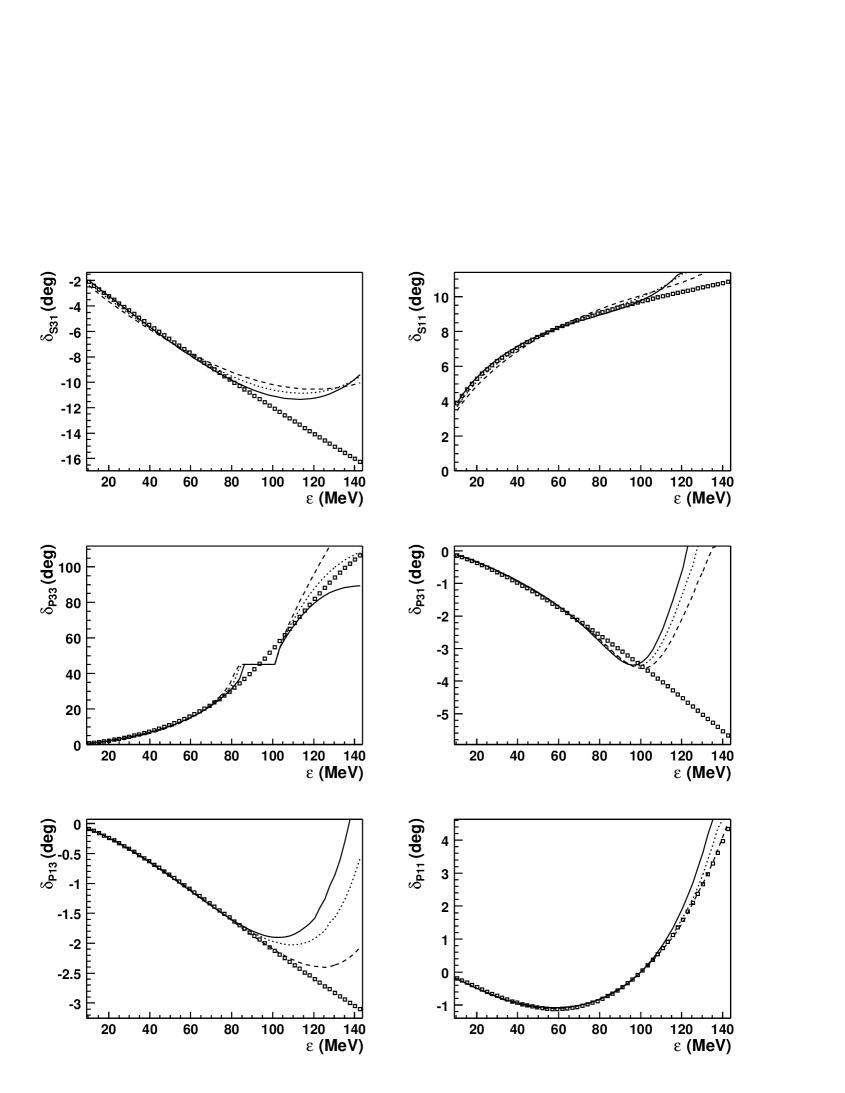
FIG. 6.: The $S$- and $P$-wave phase shifts using the $S$-matrix method as a function of the pion c.m. kinetic energy, $\epsilon$. The solid curve corresponds to an unconstrained nucleon $\sigma$ term, while for the dotted and dashed curves it is constrained to be 75 MeV and 45 MeV, respectively. The data are from Ref. [27]

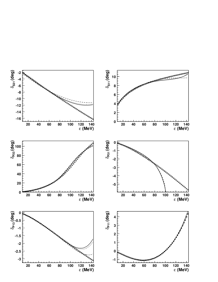
FIG. 7.: As for Fig. 6, but using the $K$-matrix method.

Our fits to the $S$- and $P$-wave phase shifts in the HB calculation are shown in Figs. 6 and 7 using the $S$-matrix and $K$-matrix methods, respectively. Here the solid curves correspond to an unconstrained fit. As in I and Ref. [10] it was possible to fit the phase shift data out to a pion c.m. kinetic energy, $\epsilon$, of 100 MeV, slightly below the $\Delta$ resonance at $\epsilon=127$ MeV. More precisely the data were fitted from $\sqrt{s}=1090$ to 1200 MeV in 3 MeV steps. The short horizontal section in Fig. 6 indicates a small region where unitarity, which is only enforced perturbatively, is slightly violated and a phase shift cannot be determined; this, of course, does not occur in the $K$-matrix approach, by definition. The corresponding parameters are collected in Table I where, in common with previous work, it is observed that the deduced values of the $\sigma$ term are much larger than the oft-quoted figure of $45\pm 8$ due to Gasser et al. [29]. Therefore we performed two additional fits where $\kappa_{2}$ was constrained to produce values of the $\sigma$ term of 75 MeV and 45 MeV. These are indicated, respectively, by the dotted and dashed curves in Figs. 6 and 7. For the $K$-matrix case the dotted curve is barely distinuishable from the solid curve since the change in the $\sigma$ term is small here.

As expected the $S$-matrix fits in Fig. 6 are quite similar to those given in I. The fitted parameters, however, differ since here we include the polynomial terms and we subsume the renormalization scale dependance into the low energy constants. In many of the partial waves the $K$-matrix fits (Fig. 7) are a little better, particularly for $\delta_{P33}$, however $\delta_{P31}$ begins to deviate significantly from the data at $\epsilon\sim 80$ MeV. Something of the same trend is visible in the work of Fettes and Meißner [10]. The ${\cal O}(Q^{2})$ low energy constants given there are related to our constants by $c_{1}=\kappa_{2}/M$, $c_{2}=\kappa_{1}/(2M)$, $c_{3}=2\beta_{\pi}/M$ and $c_{4}=\kappa_{\pi}/M$. Their fit $1^{\dagger}$ to Matsinos’ data [30] produces values which are fairly similar to ours when the different value of the $\pi N\Delta$ coupling, $h_{A}$, and the constraint $\sigma(0)=59$ MeV are taken into account. (We should note, however, that substantial differences are seen for their fit to the Karlsruhe data [31].) The ${\cal O}(Q^{2})$ constants in Table I are reasonably similar in the $S$- and $K$-matrix calculations, however sizeable differences appear at ${\cal O}(Q^{3})$. Further they are not of natural size (unity). These features may be due to the strong cancellations which occur among the various terms and the fact that the parameters are not uniquely determined since it is possible to obtain similar values of $\chi^{2}$ when $\sigma(0)$ is constrained. A significantly larger $\chi^{2}$ is only obtained for the $S$-matrix case with $\sigma(0)=45$ MeV.

TABLE I.: Low energy constants and effective couplings obtained from the $S$- and $K$-matrix fits with unconstrained and constrained values of the nucleon $\sigma$ term.

	$S$-matrix			$K$-matrix
$\beta_{\pi}$	4.78	4.46	4.13	4.06	4.06	4.05
$\kappa_{\pi}$	$-$10.1	$-$9.02	$-$7.76	$-$7.96	$-$7.79	$-$7.21
$\kappa_{1}$	$-$10.6	$-$9.80	$-$8.82	$-$9.36	$-$9.29	$-$9.04
$\kappa_{2}$	$-$0.453	$-$0.124∗	0.241∗	$-$0.234	$-$0.124∗	0.240∗
$\lambda_{1}$	23.7	16.6	8.20	9.11	7.77	3.13
$\lambda_{2}$	$-$20.1	$-$18.0	$-$15.9	$-$14.9	$-$14.7	$-$14.4
$\lambda_{3}$	$-$19.5	$-$16.8	$-$13.4	$-$14.1	$-$13.5	$-$11.6
$\lambda_{4}$	$-$21.0	$-$19.0	$-$17.1	$-$16.9	$-$16.8	$-$16.5
$\lambda_{5}$	9.14	8.03	7.20	6.03	6.00	6.01
$\lambda_{6}$	0.661	$-$3.01	$-$7.08	$-$7.32	$-$8.03	$-$10.4
$\tilde{h}_{A}$	1.24	0.918	0.543	0.612	0.548	0.329
$\chi^{2}$	0.26	0.38	0.77	0.92	0.94	1.2
$\sigma(0)$ (MeV)	102.1	75.0	45.0	84.0	75.0	45.0
$\zeta_{\pi NN}$	1.088	1.056	1.021	1.050	1.041	1.012
$\zeta_{\pi N\Delta}$	0.905	1.024	1.156	1.160	1.183	1.260

^∗ Constrained.

The ratios of the effective $\pi NN$ coupling constant to the bare value, $\zeta_{\pi NN}$, in Table I show a Goldberger-Treiman discrepancy of a few percent. Schröder et al. [32] have recently determined a precise result, namely $\zeta_{\pi NN}=1.027^{+0.012}_{-0.008}$. A similar value is obtained from the latest $\pi NN$ coupling constant obtained by the George Washington University/TRIUMF group [33]. These values favor a $\sigma$ term of between 75 and 45 MeV which is in accord with several recent analyses. In Ref. [33] 64 MeV is quoted with an error of about 10%. A sum rule determination by Olsson [34] gave 55 MeV with a 16% error. Finally Schröder et al. [32] have indicated that the value of 45 MeV extracted [29] from the Karlsruhe data should be increased by 13 MeV giving 58 MeV. Lastly we note that since $\zeta_{\pi N\Delta}$ remains fairly close to unity the coupling is not changed too much from the bare value, which seems intuitively reasonable.

TABLE II.: $S$-wave scattering lengths and $P$-wave scattering volumes in units of $m^{-1}$ and $m^{-3}$, respectively

	$S$-matrix			$K$-matrix			Experiment
$\sigma(0)$ (MeV)	102.1	75.0	45.0	84.0	75.0	45.0
$b_{0}$	0.0051	$-$0.0061	$-$0.0180	0.0016	$-$0.0024	$-$0.0155	$-0.0012\pm 0.0010$ [35]
							$-0.0034\pm 0.0007$ [36]
$b_{1}$	$-$0.0830	$-$0.0826	$-$0.0824	$-$0.0847	$-$0.0846	$-$0.0843	$-0.0895\pm 0.0016$ [35]
							$-0.0918\pm 0.0013$ [36]
$a_{11}$	$-$0.0753	$-$0.0754	$-$0.0752	$-$0.0769	$-$0.0766	$-$0.0757	$-0.078\pm 0.002$ [31]
$a_{13}$	$-$0.0290	$-$0.0289	$-$0.0282	$-$0.0281	$-$0.0280	$-$0.0276	$-0.030\pm 0.002$ [31]
$a_{31}$	$-$0.0392	$-$0.0398	$-$0.0400	$-$0.0378	$-$0.0379	$-$0.0382	$-0.046\pm 0.007$ [37]
$a_{33}$	0.2180	0.1984	0.1787	0.1966	0.1919	0.1766	$0.205\pm 0.004$ [37]

It is also interesting to examine the threshold results. We give in Table II the $S$-wave isoscalar and isovector scattering lengths, $b_{0}=(a_{1}+2a_{3})/3$ and $b_{1}=(a_{3}-a_{1})/3$ (with the notation $a_{2I}$) and the $P$-wave scattering volumes ($a_{2I\,2J}$). The experimental values come from various sources. The $S$-wave isoscalar scattering lengths were obtained [35, 36] from the pionic atom data [32] with an improved treatment of the $\pi$-$d$ scattering length. The $I={\textstyle{\frac{1}{2}}}$ $P$-wave scattering volumes are the old Karlsruhe values [31], while the $I={\textstyle{\frac{3}{2}}}$ volumes are from a recent analysis by Fettes and Matsinos [37]. Our calculated results for $b_{0}$ at the extreme values of $\sigma(0)$ are clearly not favored by the data which prefer a value in the middle. Notice that, at this level of accuracy, there is a noticeable difference between the $S$- and $K$-matrix results. The value of $a_{33}$ appears to be somewhat low for the cases where $\sigma(0)=45$ MeV. Apart from this, the remaining $P$-wave results and the values of $b_{1}$ show little sensitivity to the calculation employed and are in reasonable agreement with the data. Of course this is not surprising since the low energy phase shifts are included in the fit.

B IR Results

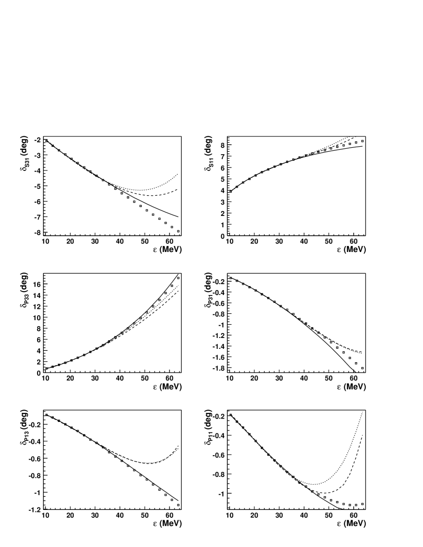
FIG. 8.: The $S$- and $P$-wave phase shifts from the $S$-matrix in the IR scheme (dashed curve) and from the $K$-matrix in the IR scheme (dotted) and HB scheme (solid) as a function of the pion c.m. kinetic energy, $\epsilon$. The data are from Ref. [27]

TABLE III.: Low energy constants, $\sigma$ term and effective couplings obtained by fitting to $\epsilon=$ 40 MeV using the $S$- and $K$-matrix in the IR scheme and the $K$-matrix in the HB scheme

	IR		HB
	$S$-matrix	$K$-matrix	$K$-matrix
$\beta_{\pi}$	4.23	5.31	6.12
$\kappa_{\pi}$	$-$10.4	$-$12.9	$-$12.0
$\kappa_{1}$	$-$10.4	$-$15.1	$-$14.5
$\kappa_{2}$	$-$0.121	$-$0.244	$-$0.287
$\lambda_{1}$	22.0	33.6	31.5
$\lambda_{2}$	$-$24.4	$-$26.9	$-$23.7
$\lambda_{3}$	$-$38.2	$-$45.3	$-$23.9
$\lambda_{4}$	$-$16.9	$-$18.9	$-$24.4
$\lambda_{5}$	18.0	18.8	7.74
$\lambda_{6}$	19.6	19.1	$-$6.00
$\tilde{h}_{A}$	0.500	0.664	1.50
$\chi^{2}$	0.075	0.066	0.025
$\sigma(0)$(MeV)	108.9	119.0	88.4
$\zeta_{\pi NN}$	0.790	0.699	1.043
$\zeta_{\pi N\Delta}$	0.378	0.381	1.079

Turning to the IR scheme the results are disappointing. It was only found possible to fit the phase shift data in the low energy regime out to $\epsilon=40$ MeV. Specifically we fitted for $\sqrt{s}$ from 1090 to 1123 MeV in steps of 3 MeV. The IR $S$-matrix results are shown by the dashed curves in Fig. 8; here the restriction $\tilde{h}_{A}\leq 0.5$ was imposed, see the discussion below. The $K$-matrix results are denoted by dotted curves in the figure. For contrast the solid line shows the HB results for a fit over the same energy range; the HB results from the $S$- and $K$-matrix methods are very similar and we choose to display the $K$-matrix results. While the HB phase shifts follow the data approximately for $\epsilon>40$ MeV, in a number of cases the IR results rapidly diverge from the experimental values. The parameters corresponding to these results are collected in Table III. While the HB parameters differ from those given in Table I, particularly those of ${\cal O}(Q^{3})$, we caution that they are not well determined by a fit over this limited energy range. Notice that, for the $K$-matrix cases, $\chi^{2}$ is substantially larger in the IR scheme than the HB one. In the IR case $\zeta_{\pi NN}$ differs substantially from unity, implying a huge Goldberger-Treiman discrepancy. This is unphysical and is a signal of the contortions that the parameters are going through in order to fit over even this limited range of energies. The quantity $\zeta_{\pi N\Delta}$ is also much less than unity implying an effective $\pi N\Delta$ coupling very different from the bare value.

TABLE IV.: Comparison of IR results for the real parts of various integrals and $\Pi_{\Delta}$ in the $s$-channel with the corresponding HB approximation.

	$\sqrt{s}=1200$ MeV		$\sqrt{s}=1100$ MeV
Integral	IR	HB	IR	HB
$\bar{{\cal I}}_{11}(s,M_{\Delta})$	0.338	0.357	0.148	0.120
$\bar{{\cal I}}_{11}^{(2)}(s,M_{\Delta})/\bar{M}^{2}$	0.00193	0.00199	0.000314	0.000192
$\bar{{\cal I}}_{12}^{(3)}(s,M_{\Delta})$	$-$0.00127	$-$0.00413	$-$0.00797	$-$0.0103
$\bar{M}^{2}\bar{{\cal I}}_{13}^{(3)}(s,0,M_{\Delta},M,M_{\Delta})$	0.0798	0.0453	0.1020	0.0568
$\Pi_{\Delta}(s)/\bar{M}^{2}$ for $\tilde{h}_{A}^{2}=0.1$	0.000287	0.00546	0.0230	0.0696

TABLE V.: Comparison of IR results for the real parts of various integrals and $\Pi_{\Delta}$ in the $u$-channel, for $u=u_{\rm min}$, with the corresponding HB approximation.

	$\sqrt{s}=1200$ MeV		$\sqrt{s}=1100$ MeV
	$\sqrt{u_{\text{min}}}=$601.7 MeV		$\sqrt{u_{\text{min}}}=$769.5 MeV
Integral	IR	HB	IR	HB
$\bar{{\cal I}}_{11}(u,M_{\Delta})$	$-$6.51	$-$1.42	$-$2.39	$-$0.934
$\bar{{\cal I}}_{11}^{(2)}(u,M_{\Delta})/\bar{M}^{2}$	1.34	0.0826	0.173	0.0316
$\bar{{\cal I}}_{12}^{(3)}(u,M_{\Delta})$	0.840	0.110	0.180	0.0500
$\bar{M}^{2}\bar{{\cal I}}_{13}^{(3)}(u,0,M_{\Delta},M,M_{\Delta})$	0.597	0.167	0.321	0.130
$\Pi_{\Delta}(u)/\bar{M}^{2}$ for $\tilde{h}_{A}^{2}=0.1$	$-$0.751	0.319	0.0213	0.262

We have, of course, carried out a number of additional IR calculations with a view to improving the results. For example constraining the value of the $\sigma$ term to be 75 or 45 MeV increases the value of $\chi^{2}$, but the results are qualitatively very similar to those discussed above. In order to see whether the problem was due to the $\Delta$ resonance contributions we removed them entirely by setting the coupling $h_{A}$ to zero. As expected the parameters changed substantially, but the fit to the phase shifts remained qualitatively the same and in fact $\chi^{2}$ increased somewhat. Thus we have not been able to qualitatively improve the IR results discussed in detail above.

In order to further investigate the reason for the problem with the IR approach we compare the IR polarization $\Pi_{\Delta}$ of Eq. (27) and a few IR integrals (defined in the Appendix) with their HB counterparts. In Table IV we make the comparison in the $s$-channel. For the most part the IR and HB results are quite comparable. The picture changes for the $u$-channel in Table V, where for a given $s$ we have chosen the minimum value, $u_{\rm min}=2(M^{2}+m^{2})-s$, so as to enhance the contrast. Here the IR integrals are much larger than the corresponding HB results, by a factor of 6 on average. Further $\Pi_{\Delta}(u)$ changes sign. Since $\Delta_{R}(u)=1/[u-M_{\Delta}^{2}-\Pi_{\Delta}(u)]$ and $u-M_{\Delta}^{2}$ is negative this change of sign can produce a pole; this was the reason for our restriction of $\tilde{h}_{A}\leq 0.5$ in the $S$-matrix IR fit. Of course the problem does not arise if $\Pi_{\Delta}(u)$ is expanded out of the denominator as in the $K$-matrix approach, although the mathematical justification for doing so is slight. The problem does not arise in the HB case where $\Pi_{\Delta}(u)$ is always positive.

It is also useful to make the point graphically by studying the basic integral involving one baryon and one meson propagator. Figure 9 shows $\bar{\cal I}_{11}(s,M_{\Delta})$ as a function of $\sqrt{s}$. It is observed that the IR integral (solid line) and the HB approximation thereto (dashed curve) agree quite closely. Figure 10 shows the corresponding result in the $u$-channel; $\bar{\cal I}_{11}(u_{\rm min},M_{\Delta})$ as a function of $\sqrt{s}$. It is seen that the magnitude of the IR integral (solid line) is much larger than that of its HB counterpart (dashed curve); note the ordinate scale here in comparison to Fig. 9. The IR integral is governed by the value of $x$ (see Appendix) which in the $s$-channel is $(s-M_{\Delta}^{2}+m^{2})/(2m\sqrt{s})$. In the HB approximation this is replaced by $(s-M_{\Delta}^{2})/(2m\bar{M})=(\eta-\delta)/m$, in the notation of I. At $\sqrt{s}=1200$ MeV, $x$ is $-0.18$ ($-0.26$) in the IR (HB) case. Correspondingly in the $u$-channel, at $\sqrt{u_{\rm min}}=601.7$ MeV, $x$ is $-6.79$ ($-3.83$) in the IR (HB) case and this large difference is the heart of the problem with the IR approach. However, it is disquieting that the rather reasonable HB results are achieved by the replacement of $\sqrt{u}$ in the denominator by the square root of average baryon mass, $\sqrt{\bar{M}}$, since this can be quite a rough approximation.

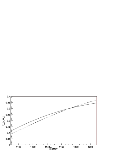
FIG. 9.: Comparison of the integral $\bar{{\cal I}}_{11}(s,M_{\Delta})$ evaluated exactly (solid curve) with the HB approximation (dashed curve) as a function of $\sqrt{s}$.

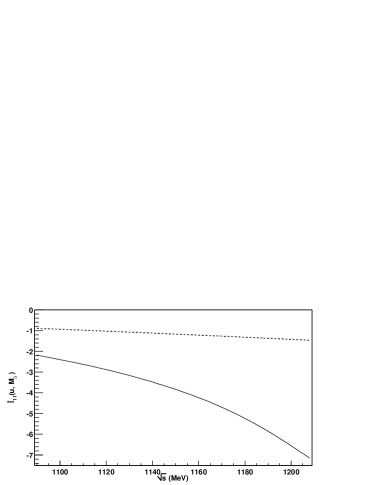
FIG. 10.: Comparison of the integral $\bar{{\cal I}}_{11}(u,M_{\Delta})$, for $u=u_{\rm min}$, evaluated exactly (solid curve) with the HB approximation (dashed curve) as a function of $\sqrt{s}$.

IV Conclusions

We have performed a least-squares fit to the $S$- and $P$-wave phase shift data using chiral perturbation theory to ${\cal O}(Q^{3})$ with explicit $\pi$, $N$ and $\Delta$ fields. The heavy baryon formulation used here represents an improvement compared to I in that the polynomial terms were included explicitly and the renormalization scale dependance was subsumed into the low energy constants. We contrasted an “$S$-matrix” method (as in I) with a $K$-matrix analysis (as in Ref. [10]). The former seems to be more physical since it employs dressed $\Delta$ propagators which are finite, while the latter uses bare propagators which give a divergent scattering amplitude at the $\Delta$ resonance energy. Broadly speaking the two methods give similar results and allow a fit to the phase shift up to a c.m. pion kinetic energy, $\epsilon$, of 100 MeV. In detail, however, there are some differences. For instance, the value of the $\sigma$ term (if unconstrained) and the Goldberger-Treiman discrepancy are smaller with the $K$-matrix.

Our main interest was to see whether the infrared regularization scheme, which is manifestly Lorentz invariant, could provide an equally satisfactory account of the phase shift data. It could not. We were only able to fit the data up to $\epsilon=40$ MeV and the resulting Goldberger-Treiman discrepancy was ridiculously large. The difficulty was not due to the explicit inclusion of the $\Delta$ resonance, but rather stemmed from the $u$ channel where the magnitudes of the integrals were much larger than the corresponding heavy baryon ones. This leads to uneasiness regarding the latter since they are obtained by approximating the former. The heavy baryon scheme thus pushes significant contributions into higher orders where they are combined with the other terms of that order. The only information we have as to whether the net effect is small comes from the comparison of third and fourth orders carried out by Fettes and Meißner [12]. In some cases there are sizeable differences, although these authors suggest that in most cases the chiral series appears convergent. Overall, in our opinion, the description of pion-nucleon scattering via chiral perturbation theory is not yet in a satisfactory state.

Integrals involving only meson propagators need no discussion since the standard results are used and integrals involving only baryon propagators give no contribution in the IR or HB schemes. Infrared regularization is needed for integrals involving both baryon and meson propagators. Here we give only those integrals that are referred to in the main text, together with their HB reduction. The integrals needed can be derived from the basic infrared integral which has been discussed by Becher and Leutwyler [6] (note that our conventions differ from theirs), see also I. Explicitly this is

$$i\mu^{4-d}\int_{I}\frac{d^{d}\ell}{(2\pi)^{d}}\frac{1}{[(\ell+k)^{2}-{\cal M}^{2}+i\epsilon][\ell^{2}-m^{2}+i\epsilon]}$$ (54)

$$=i\mu^{4-d}\int\frac{d^{d}\ell}{(2\pi)^{d}}\frac{1}{[2k\cdot\ell+k^{2}-{\cal M}^{2}+m^{2}+i\epsilon][\ell^{2}-m^{2}+i\epsilon]}$$ (55)

$$={\cal I}_{11}^{L}(s,{\cal M})+(4\pi)^{-2}\bar{\cal I}_{11}(s,{\cal M})\;,$$ (56)

where $s=k^{2}$. The total integral, without the subscript $I$, will have, in addition to the infrared part, a regular part but this can be discarded since it can be expanded with the various terms absorbed into the low energy constants. The divergent IR contribution is

$${\cal I}_{11}^{L}(s,{\cal M})=\frac{(s-{\cal M}^{2}+m^{2})}{2s}\left[2L+\frac{1}{(4\pi)^{2}}\ln\frac{m^{2}}{\mu^{2}}\right]\;,$$ (57)

$${\rm where}\quad L=\frac{1}{32\pi^{2}}\left(\frac{2}{d-4}+\gamma-1-\ln 4\pi\right)\;,$$ (58)

with $\gamma$ denoting Euler’s constant. The real part of the finite piece is

$$\Re\bar{\cal I}_{11}(s,{\cal M}) = \left\{\matrix{\frac{m}{\sqrt{s}}\left[-x+2\sqrt{1-x^{2}}\cos^{-1}(-x)\right]&\qquad(|x|\leq 1)\cr\frac{m}{\sqrt{s}}\left[-x+\sqrt{x^{2}-1}\ln\frac{x+\sqrt{x^{2}-1}}{x-\sqrt{x^{2}-1}}\right]&\qquad(|x|\geq 1)\cr}\right.$$ (59)

$$\rightarrow -\frac{1}{\bar{M}}J\left(\frac{s-{\cal M}^{2}}{2\bar{M}}\right)\;,$$ (60)

where $x=(s-{\cal M}^{2}+m^{2})/(2m\sqrt{s})$. The last line here makes contact with the HB integral $J$ in I for which $\sqrt{s}$ in the denominator is approximated in leading order by the average baryon mass $\bar{M}={\textstyle{\frac{1}{2}}}(M+M_{\Delta})$. The imaginary part of the IR integral is

$$\Im\bar{\cal I}_{11}(s,{\cal M})=-\frac{\pi}{s}\sqrt{(s-{\cal M}^{2}+m^{2})^{2}-4sm^{2}}\>\theta(s-[{\cal M}+m]^{2})\;,$$ (61)

where $\theta$ denotes the Heaviside step function.

In the following we shall implictly give only the real part of the IR integral and the $i\epsilon$ in the integrand denominators will be suppressed. For the integral

$$i\mu^{4-d}\int_{I}\frac{d^{d}\ell}{(2\pi)^{d}}\frac{\ell_{\mu}}{[(\ell+k)^{2}-{\cal M}^{2}][\ell^{2}-m^{2}]}={\cal I}_{11}^{(1)}(s,{\cal M})k_{\mu}\;.$$ (62)

The finite part is $(4\pi)^{-2}\bar{\cal I}_{11}^{(1)}$, with

$$\bar{\cal I}_{11}^{(1)}(s,{\cal M})=-\left[\frac{s-{\cal M}^{2}+m^{2}}{2s}\right]\bar{\cal I}_{11}(s,{\cal M})\rightarrow\left[\frac{s-{\cal M}^{2}}{2\bar{M}^{3}}\right]J\left(\frac{s-{\cal M}^{2}}{2\bar{M}}\right)\;,$$ (63)

with the last expression giving the HB reduction.

For the integral

$$i\mu^{4-d}\int_{I}\frac{d^{d}\ell}{(2\pi)^{d}}\frac{\ell_{\mu}\ell_{\nu}}{[(\ell+k)^{2}-{\cal M}^{2}][\ell^{2}-m^{2}]}={\cal I}_{11}^{(2)}(s,{\cal M})g_{\mu\nu}+{\cal I}_{11}^{(3)}(s,{\cal M})k_{\mu}k_{\nu}\;.$$ (64)

The finite part of the first term is $(4\pi)^{-2}\bar{\cal I}_{11}^{(2)}$, with

$$\bar{\cal I}_{11}^{(2)}(s,{\cal M}) = \left[\frac{4m^{2}s-(s-{\cal M}^{2}+m^{2})^{2}}{12s}\right]\bar{\cal I}_{11}(s,{\cal M})-\frac{(s-{\cal M}^{2})}{36s^{2}}\left[6m^{2}s-(s-{\cal M}^{2})^{2}\right]$$ (65)

$$\rightarrow -\frac{1}{3\bar{M}}\left[m^{2}\!-\frac{(s-{\cal M}^{2})^{2}}{4\bar{M}^{2}}\right]\!J\!\left(\frac{s-{\cal M}^{2}}{2\bar{M}}\right)-\frac{(s-{\cal M}^{2})}{18\bar{M}^{2}}\left[3m^{2}\!-\frac{(s-{\cal M}^{2})^{2}}{2\bar{M}^{2}}\right],$$ (66)

with the last line giving the HB reduction.

One of the integrals involving one pion and two baryon denominators is

$$i\mu^{4-d}\int_{I}\frac{d^{d}\ell}{(2\pi)^{d}}\frac{\ell_{\mu}\ell_{\nu}}{[(\ell+p^{\prime}+q^{\prime})^{2}-{\cal M}_{A}^{2}][(\ell+p^{\prime})^{2}-{\cal M}_{B}^{2}][\ell^{2}-m^{2}]}$$ (67)

$$={\cal I}_{12}^{(3)}(s,{\cal M}_{A},{\cal M}_{B})g_{\mu\nu}+\ldots\;.$$ (68)

The finite part is $(4\pi)^{-2}\bar{\cal I}_{12}^{(3)}$, with

$$\bar{{\cal I}}_{12}^{(3)}(s,{\cal M}_{A},{\cal M}_{B})=\left(\frac{\partial}{\partial{\cal M}_{A}^{2}}+\frac{\partial}{\partial{\cal M}_{B}^{2}}\right)\int\limits_{0}^{1}dz\,\bar{{\cal I}}_{11}^{(2)}(\bar{k}^{2},\bar{\cal M})\;,$$ (69)

$${\rm where}\quad\bar{k}^{2}=m^{2}z^{2}+(s-M^{2}-m^{2})z+M^{2}\;,$$ (70)

$${\rm and}\quad\bar{\cal M}^{2}=m^{2}z^{2}+({\cal M}_{A}^{2}-{\cal M}_{B}^{2}-m^{2})z+{\cal M}_{B}^{2}\;.$$ (71)

This was evaluated by performing the differentiation analytically and carrying out the integration numerically using Gaussian quadrature. It is reduced to HB form by dropping terms involving $m^{2}$ from the expression $\quad\bar{k}^{2}-\bar{\cal M}^{2}+m^{2}$ and setting $\quad\bar{k}^{2}\simeq M^{2}$ in denominators. This allows the integral to be performed, giving

$$\bar{{\cal I}}_{12}^{(3)}(s,M_{\Delta},M)\rightarrow-\frac{1}{6\bar{M}^{2}}\left[F_{3}(\eta-\delta,0)-m^{2}+{\textstyle{\frac{2}{3}}}(\eta-\delta)^{2}\right]\;,$$ (72)

$${\rm where}\quad F_{3}(\alpha,\beta)=\frac{1}{\alpha-\beta}\left[(\alpha^{2}-m^{2})J(\alpha)-(\beta^{2}-m^{2})J(\beta)\right]\;,$$ (73)

and we recall the definitions of I: $2\bar{M}\eta=s-M^{2}$ and $\delta=M_{\Delta}-M$.

The integral involving one pion and three baryon denominators is

$$i\mu^{4-d}\int_{I}\frac{d^{d}\ell}{(2\pi)^{d}}\frac{\ell_{\mu}\ell_{\nu}}{[(\ell+p^{\prime})^{2}-{\cal M}_{A}^{2}][(\ell+p^{\prime}+q^{\prime})^{2}-{\cal M}_{B}^{2}][(\ell+p)^{2}-{\cal M}_{C}^{2}][\ell^{2}-m^{2}]}$$ (74)

$$={\cal I}_{13}^{(3)}(s,t,{\cal M}_{A},{\cal M}_{B},{\cal M}_{C})g_{\mu\nu}+\ldots\;.$$ (75)

The finite part is $(4\pi)^{-2}\bar{\cal I}_{13}^{(3)}$, with

$$\bar{{\cal I}}_{13}^{(3)}(s,t,{\cal M}_{A},{\cal M}_{B},{\cal M}_{C})=\left(\frac{\partial}{\partial{\cal M}_{A}^{2}}+\frac{\partial}{\partial{\cal M}_{B}^{2}}+\frac{\partial}{\partial{\cal M}_{C}^{2}}\right)^{\!2}\int\limits_{0}^{1}dxx\int\limits_{0}^{1}dy\,\bar{\cal I}_{11}^{(2)}(\bar{k}^{2},\bar{\cal M})$$ (76)

$${\rm where}\quad\bar{k}^{2}=\left[s-M^{2}-m^{2}+m^{2}x(1-y)\right]x(1-y)-txy(1-x)+M^{2}\;,$$ (77)

$${\rm and}\quad\bar{\cal M}^{2}=m^{2}x^{2}(1-y)^{2}+\left[{\cal M}_{A}^{2}-{\cal M}_{B}^{2}+m^{2}-t(1-x)\right]xy$$ (78)

$$\qquad\qquad\qquad+({\cal M}_{B}^{2}-{\cal M}_{C}^{2}-m^{2})x+{\cal M}_{C}^{2}\;.$$ (79)

This was evaluated with a combination of numerical differentiation and Gaussian numerical integration. The HB reduction is carried out by making similar approximations to those mentioned above and this allows both integrals to be performed. For the cases mentioned in the text this gives

$$\bar{{\cal I}}_{13}^{(3)}(s,t,M_{\Delta},M,M_{\Delta})\rightarrow\frac{1}{12\bar{M}^{3}}\left[F_{1}(\eta,-\delta)+{\textstyle{\frac{2}{3}}}(\eta-2\delta)\right]\;,$$ (80)

$${\rm where}\quad F_{1}(\alpha,\beta)=\frac{(\alpha^{2}-m^{2})J(\alpha)+(2\beta^{2}-3\alpha\beta+m^{2})J(\beta)+(\alpha-\beta)(2\beta^{2}-m^{2})}{(\alpha-\beta)^{2}}\,,$$ (81)

and

$$\bar{{\cal I}}_{13}^{(3)}(s,t,M_{\Delta},M,M)\rightarrow\frac{1}{12\bar{M}^{3}}\left[F_{2}(\eta,-\delta)+{\textstyle{\frac{2}{3}}}(\eta-\delta)\right]\;,$$ (82)

$${\rm where}\quad F_{2}(\alpha,\beta)=\frac{(\alpha^{2}-m^{2})\beta J(\alpha)-(\beta^{2}-m^{2})\alpha J(\beta)+\pi m^{3}(\alpha-\beta)}{\alpha\beta(\alpha-\beta)}\,.$$ (83)

REFERENCES

- [1] S. Weinberg, Physica A 96, 327 (1979).
- [2] J. Gasser and H. Leutwyler, Ann. Phys. (NY) 158, 142 (1984); for a recent review see H. Leutwyler, At the Frontier of Particle Physics: Handbook of QCD, edited by M. Shifman (World Scientific, Singapore, 2001) Vol. 1, p.271.
- [3] H. Leutwyler, in QCD@Work, Int. Workshop on Quantum Chromodynamics: Theory and Experiment, edited by P. Colangelo and G. Nardulli (Martina Franca, Italy, 2001) AIP Conf. Proc. 602, 3 (2001).
- [4] J. Gasser, M.E. Sainio and A. Švarc, Nucl. Phys. B 307, 779 (1988).
- [5] E. Jenkins and A.V. Manohar, Phys. Lett. B 255, 558 (1991).
- [6] T. Becher and H. Leutwyler, Eur. Phys. J. C 9, 643 (1999).
- [7] P.J. Ellis and H. B. Tang, Phys. Rev. C 57, 3356 (1998).
- [8] P.J. Ellis and K. Torikoshi, Phys. Rev. C 61, 015205 (2000); B. Kubis and Ulf-G. Meißner, Nucl. Phys. A 679, 698 (2001); Eur. Phys. J. C 18, 747 (2001); V. Bernard, T.R. Hemmert and Ulf-G. Meißner, Phys. Lett. B 545, 105 (2002); B. Borasoy and S. Wetzel, Phys. Rev. D 63, 074019 (2001); N. Beisert and B. Borasoy, Nucl. Phys. A 705, 433 (2002).
- [9] Ulf-G. Meißner, At the Frontier of Particle Physics: Handbook of QCD, edited by M. Shifman (World Scientific, Singapore, 2001) Vol. 1, p.417.
- [10] N. Fettes and Ulf-G. Meißner, Nucl. Phys. A 679, 629 (2001).
- [11] N. Fettes, Ulf-G. Meißner and S. Steininger, Nucl. Phys. A 640, 199 (1998).
- [12] N. Fettes and Ulf-G. Meißner, Nucl. Phys. A 676, 311 (2000).
- [13] P.J. Ellis, in Chiral Dynamics: Theory and Experiment III, edited by A.M. Bernstein, J.L. Goity and Ulf-G. Meißner (Jefferson Laboratory, Newport News, VA, 2000) World Scientific, Singapore (2001), p. 356.
- [14] N. Fettes and Ulf-G. Meißner, Phys. Rev. C 63, 045201 (2001); Nucl. Phys. A 693, 693 (2001).
- [15] T. Becher and H. Leutwyler, J. High Energy Phys. 06, 017 (2001).
- [16] S. Weinberg, Phys. Lett. B 251, 288 (1990); Nucl. Phys. B 363, 3 (1991).
- [17] V. Pascalutsa, Phys. Rev. D 58, 096002 (1998); V. Pascalutsa and R. Timmermans, Phys. Rev. C 60, 042201 (1999).
- [18] H.-B. Tang and P.J. Ellis, Phys. Lett. B 387, 9 (1996).
- [19] G. Höhler, Pion-Nucleon Scattering, Landolt-Börnstein, New Series, ed. H. Schopper, Vol. I/9 b2 (Springer-Verlag, Berlin, 1983).
- [20] P. Van Nieuwenhuizen, Phys. Rep. 68, 189 (1981).
- [21] M. Benmerrouche, R.M. Davidson and N.C. Mukhopadhyay, Phys. Rev. C39, 2339 (1989).
- [22] S. Gasiorowicz, Elementary Particle Physics (John Wiley & Sons, New York, 1966).
- [23] T. Ericson and W. Weise, Pions and Nuclei (Oxford University Press, New York, 1988).
- [24] P.J. Ellis and H.-B. Tang, Phys. Rev. C56, 3363 (1997).
- [25] M. Mojžiš, Eur. Phys. J. C2, 181 (1998).
- [26] Particle Data Group, D.E. Groom et al., Eur. Phys. J. C 15, 1 (2000).
- [27] R.A. Arndt et al., SAID online program at http://gwdac.phys.gwu.edu/, solution SM01.
- [28] Ulf-G. Meißner and J.A. Oller, Nucl. Phys. A 673, 311 (2000).
- [29] J. Gasser, H. Leutwyler and M.E. Sainio, Phys. Lett. B 253, 252 (1991).
- [30] E. Matsinos, Phys. Rev. C 56, 3014 (1997).
- [31] R. Koch, Nucl. Phys. A 448, 707 (1986); scattering volume errors taken from R. Koch and E. Pietarinen, Nucl. Phys. A 336, 331 (1980).
- [32] H.-Ch. Schröder, A. Badertscher, P.F.A. Goudsmit, M. Janousch, H.J. Leisi, E. Matsinos, D. Sigg, Z.G. Zhao, D. Chatellard, J.-P. Egger, K. Gabathuler, P. Hauser, L.M. Simons and A.J. Rusi El Hassani, Eur. Phys. J. C 21, 473 (2001).
- [33] M.M. Pavan, R.A. Arndt, I.I. Strakovsky and R.L. Workman, hep-ph/0111066, PiN Newslett. 16, 110 (2002).
- [34] M.G. Olsson, Phys. Lett. B 482, 50 (2000).
- [35] T.E.O. Ericson, B. Loiseau and A.W. Thomas, Phys. Rev. C 66, 014005 (2002).
- [36] S.R. Beane, V. Bernard, E. Epelbaum, Ulf-G. Meißner and D.R. Phillips, hep-ph/0206219.
- [37] N. Fettes and E. Matsinos, Phys. Rev. C 55, 464 (1997).