Two-Body Dirac Equations for Nucleon-Nucleon Scattering

Abstract

We investigate the nucleon-nucleon interaction by using the meson exchange model and the two-body Dirac equations of constraint dynamics. This approach to the two-body problem has been successfully tested for QED and QCD relativistic bound states. An important question we wish to address is whether or not the two-body nucleon-nucleon scattering problem can be reasonably described in this approach as well. This test involves a number of related problems. First we must reduce our two-body Dirac equations exactly to a Schrödinger-like equation in such a way that allows us to use techniques to solve them already developed for Schrödinger-like systems in nonrelativistic quantum mechanics. Related to this we present a new derivation of Calogero’s variable phase shift differential equation for coupled Schrödinger-like equations. Then we determine if the use of  nine meson exchanges in our equations give a reasonable fit to the experimental scattering phase shifts for $n-p$ scattering. The data involves seven angular momentum states including the singlet states ${}^{1}S_{0}$, ${}^{1}P_{1}$, ${}^{1}D_{2}$ and the triplet states ${}^{3}P_{0}$, ${}^{3}P_{1}$, ${}^{3}S_{1}$, ${}^{3}D_{1}$. Two models that we have tested give us a fairly good fit. The parameters obtained by fitting the $n-p$ experimental scattering phase shift give a fairly good prediction for most of the $p-p$ experimental scattering phase shifts examined (for the singlet states ${}^{1}S_{0}$, ${}^{1}D_{2}$ and triplet states ${}^{3}P_{0}$, ${}^{3}P_{1}$). Thus the two-body Dirac equations of constraint dynamics present us with a fit that encourages the exploration of a more realistic model. We outline generalizations of the meson exchange model for invariant potentials that may possibly improve the fit.

I
Introduction

In this paper liu ,  we obtain a semi-phenomenological relativistic potential model for nucleon-nucleon interactions by using two-body Dirac equations of  constraint dynamics van1 ; c1 ; c2 ; c3 ; c4 , Saz1 and Yukawa’s theory of meson exchange.  In previous work Long and Crater long1 have derived the two-body Dirac equations for all non-derivative Lorentz invariant interactions acting together or in any combinations. They also reduced the two-body Dirac equations to coupled Schrödinger-like equations in which the potentials appear as covariant generalizations of the standard spin dependent interactions appearing in the early phenomenological works in this area 1 ; 2 ; 3 ; 4 ; 5 ; 6 ; 7 based on the nonrelativistic Schrödinger equation. This allows us to take advantage of earlier work done by other people on the nonrelativistic Schrödinger equation. In particular we use the variable phase method developed by Calogero and Degasparis cal ; dega for computation of the phase shift from the nonrelativistic Schrödinger equation, presenting a new derivation for the case of coupled equations. Our potentials for different angular momentum states are constructed from combinations of several different meson exchanges. Furthermore, our potentials, as well as the whole equations, are local, yet at the same time covariant. This contrasts our approach with other relativistic schemes such as those by Gross and others gross1 ; gross2 ; stoks ; mac . It is the aim of this paper to see if the meson exchanges we use are adequate to describe the elastic nucleon-nucleon interactions from low energy to high energy ($<$350 MeV) when using them together with two-body Dirac equations of constraint dynamics.

Although numerous relativistic approaches have been used in the nucleon-nucleon scattering problem, none of the other approaches have been tested nonperturbatively in both QED and QCD as they have been with the two-body Dirac equations of  constraint dynamics c2 ; c4 ; c6 ; c7 ; c15 . Unlike the earlier local two-body approaches of Breit Breit1 ; Breit2 ; Breit3 , the relativistic spin corrections need not be treated only perturbatively. This means that we can use nonperturbative methods (numerical methods) to solve the two-body Dirac equations. This is a very important advantage of the constraint two-body Dirac equations (CTBDE). The successful numerical tests in QED and QCD gives us confidence that they may be appropriate relativistic equations for phase shift analysis of nucleon-nucleon scattering.

In section II we introduce the two-body Dirac equations of constraint dynamics. In section III we obtain the Pauli reduction of the two-body Dirac equations to coupled Schrödinger-like equations. We go a step further than that achieved in the paper of Long and Crater in that we eliminate the first derivative terms that appear in the Schrödinger-like equation.  This is relatively simple for the case of uncoupled equations but not so for the case of coupled Schrödinger-like equations. The reason we perform this extra reduction is that the formulae we use for the phase shift analysis, the variable phase method developed by Calogero, has been worked out already for coupled equations, but ones in which the first derivative terms are absent.  This step then becomes an important part of the formalism, allowing us take advantage of previous work. In section IV, we discuss the phase shift methods used in our numerical calculations, which include phase shift equations for uncoupled and coupled states and the phase shift equations with Coulomb potential. In section V we present the models used in our calculations, including the expressions for the scalar, vector and pseudoscalar interactions, and the way they enter into our two-body Dirac equations with the mesons used in our fits. In section VI we present the results we have acheived and in section VII are the summaries and conclusions of our work.

II
Review of Constraint two-body Dirac Equations

The two-body Dirac equations that we will use for studying nucleon-nucleon interaction bear a close relation to the single particle equation proposed by Dirac in 1928 Dirac .

$$\left[\mathbf{\alpha\cdot p}+\beta m+V(r)\right]\psi=E\psi.$$ (2.1)

For interactions that transforms as a time-component of a four vector and world scalar we have $V(r)=A(r)+\beta S(r)$. Of course, the single particle Dirac equation is not suitable to describe systems such as the mesons, (quarkonium), muonium, positronium, the deuteron and nucleon-nucleon scattering because the particles may have equal or near equal mass.

The earliest attempt at putting both particles on an equal footing was in 1929 by G. Breit Breit1 Breit2 Breit3 $.~{}~{}$However, the Breit equations do not retain manifest covariant form and in QED the equations cannot be treated nonperturbatively beyond the Coulomb term Breit2 ; bse .  There have been many attempts to by pass the problems of the Breit equation and also of the full four dimensional Bethe-Salpeter equation.  These are discussed in a number of different contexts in c1 ; c2 ; c3 ; c4 .  The approach of the CTBDE provides a manifestly covariant yet three dimensional detour around many of the problems that hamper the implementation and application of Breit’s two-body Dirac equations as well as the full four dimensional Bethe-Salpeter equation (see also c10 ).  In addition, as mentioned above, the approach can by a Pauli reduction give us a local Schrödinger-like equation.

The CTBDE make use of Dirac’s relativistic Hamiltonian formalism. In a series of papers (in addition to those cited above see also c9 ; c8 ) Crater and Van Alstine have incorporated Todorov’s effective particle idea developed in his quasipotential approach Tod1 into the framework of Dirac’s Hamiltonian constraint mechanics dirac2 for a description of two body systems. Their approach yields manifestly covariant coupled Dirac equations. The standard reduction of the Breit equation to a Schrödinger-like equation for QED yields highly singular operators (like $\delta$ functions and attractive $1/r^{3}$ potentials) that can only be treated perturbatively. In the treatment of the CTBDE for QED c8 ; c6 , for example, one finds that all the operators are quantum mechanically well defined so that one can therefore use nonperturbative techniques (analytic as well as numerical) to obtain solutions of bound state problems and scattering. (A quantum mechanically well defined potential is one no more singular than $-1/4r^{2}$. If it is not quantum mechanically well defined, it can only be treated perturbatively.) Although it is encouraging that good results have been obtained for QED and QCD meson spectroscopy, that is no guarantee that the formalism so developed will lead to effective potentials in the case of nucleon-nucleon scattering that render reasonable fits to the phase shift data.

Using techniques developed by Dirac to handle constraints in quantum mechanics and the method developed by Crater and Van Alstine, one can derive the two-body Dirac equations for eight nonderivative Lorentz invariant interactions acting separately or together c12 ,long1 . These include world scalar, four vector and pseudoscalar interactions among others. We can also reduce the two-body Dirac equations to coupled Schrödinger-like equations even with all these interactions acting together. Before we test this method in nuclear physics in the phase shift analysis of the nucleon-nucleon scattering problems we review highlights of the constraint formalism and the form of the two-body Dirac equations.

II.1 Hamiltonian Formulation Of The Two-Body Problem From Constraint Dynamics

Dirac dirac2 extended Hamiltonian mechanics to include conjugate variables related by constraints of the form $\phi(q,p)=0$. For $N$ constraints, we may write

$$\phi_{n}(q,p)\approx 0,\,\,\,\,\,\,n=1,2,3,\cdot\cdot,N$$ (2.2)

With these constraints the Hamiltonian of the system (with sum over repeated indices)

$$H=\dot{q}_{n}p_{n}-L$$ (2.3)

is not unique.  The Dirac Hamiltonian $\mathcal{H~{}}$includes the constraints

$$\mathcal{H=}H+\lambda_{n}\phi_{n}.$$ (2.4)

in which $H$ is the Legendre Hamiltonian obtained from the Lagrangian by means of a Legendre transformation. The $\lambda_{n}$ may be functions of conjugate variables $q^{\prime}s$ and $p^{\prime}s$. The equation of motion for any arbitrary function $g$ (without explicit time dependence) of the conjugate variables $q^{\prime}s$ and $p^{\prime}s$ is then

$$\overset{\cdot}{g}=[g,\mathcal{H}].$$ (2.5)

Dirac called the conditional equality, $\approx$ a “ weak ” equality meaning the constraints $\phi_{n}\approx 0$ must not be applied before working out the Poisson brackets. Dirac called $=$ a nonconditional equality or a “ strong ” equality. The equations of motion are

$$\overset{\cdot}{g}=[g,\mathcal{H}]=[g,H+\lambda_{n}\phi_{n}]=[g,H]+\lambda_{n}[g,\phi_{n}]+[g,\lambda_{n}]\phi_{n}\approx[g,H]+\lambda_{n}[g,\phi_{n}]$$ (2.6)

for $\phi_{n}\approx 0$.

In the two body system, we have two constraints $\phi_{n}(q,p)\approx 0,~{}n=1,2$.  For spinless particles they are taken to be the generalized mass shell constraints of the two particles c8 ,Wong1 , namely

$$\mathcal{H}_{1}=p_{1}^{2}+m_{1}^{2}+\Phi_{1}(x,p_{1},p_{2})\approx 0,$$

$$\mathcal{H}_{2}=p_{2}^{2}+m_{2}^{2}+\Phi_{2}(x,p_{1},p_{2})\approx 0,$$ (2.7)

where

$$x=x_{1}-x_{2}.$$ (2.8)

Dirac extended his idea of handling constraints in classical mechanics to quantum mechanics by replacing the classical constraints $\phi_{n}(q,p)\approx 0$ with quantum wave equations $\phi_{n}(q,p)\mid\psi\rangle=0$, where $q$ and $p$ are conjugate variables. Thus the quantum forms for each individual particle constraint become Schrödinger-type equations saz4

$$\mathcal{H}_{i}|\psi\rangle=0{~{}~{}~{}~{}~{}~{}\mathrm{for~{}~{}~{}~{}~{}~{}~{}~{}~{}}}i=1,2.$$ (2.9)

The total Hamiltonian $\mathcal{H}$ from these constraints alone is

$$\mathcal{H=\lambda}_{1}\mathcal{H}_{1}+\lambda_{2}\mathcal{H}_{2},$$ (2.10)

(with $\lambda_{i}$ as Lagrange multipliers).  In order that each of these constraints be conserved in time we must have

$$[\mathcal{H}_{i},\mathcal{H}]|\psi\rangle=i\frac{d\mathcal{H}_{i}}{d\tau}|\psi\rangle=0.$$ (2.11)

so that

$$[\mathcal{H}_{i},\mathcal{\lambda}_{1}\mathcal{H}_{1}+\lambda_{2}\mathcal{H}_{2}]|\psi\rangle=$$

$$\{[\mathcal{H}_{i},\lambda_{1}]\mathcal{H}_{1}|\psi\rangle+\lambda_{1}[\mathcal{H}_{i},\mathcal{H}_{1}]|\psi\rangle+[\mathcal{H}_{i},\lambda_{2}]\mathcal{H}_{2}|\psi\rangle+\lambda_{2}[\mathcal{H}_{i},\mathcal{H}_{2}]\}|\psi\rangle=0.$$ (2.12)

Using Eq.(2.9), the above equation leads to this compatibility condition between the two constraints

$$[\mathcal{H}_{1},\mathcal{H}_{2}]|\psi\rangle=0.$$ (2.13)

This condition guarantees that with the Dirac Hamiltonian, the system evolves such that the “ motion ” is constrained to the surface of the mass shell described by the constraints of $\mathcal{H}_{1}$ and $\mathcal{H}_{2}$ $($Wong1 ,c8 ; c9 $).$ As described most recently in Wong1 this requires that

$$\Phi_{1}=\Phi_{2}=\Phi(x_{\perp})$$ (2.14)

(a kind of relativistic Newton’s third law) with the transverse coordinate defined by

$$x_{\nu\perp}=x_{12}^{\mu}(\eta_{\mu\nu}-P_{\mu}P_{\nu}/P^{2}),$$ (2.15)

and total momentum by

$$P=p_{1}+p_{2}.$$ (2.16)

To complete our review of the spinless case (Wong1 ) and establish notation we introduce the transverse relative momentum

$$p=\frac{\varepsilon_{2}}{w}p_{1}-\frac{\varepsilon_{1}}{w}p_{2}$$ (2.17)

$$P\cdot p=0,$$ (2.18)

where the CM energy eigenvalue $w$ is defined from

$$\left\{P^{2}+w^{2}\right\}|\psi\rangle=0.$$ (2.19)

Taking the difference of the two constraints,

$$(p_{1}^{2}-p_{2}^{2})|\psi\rangle=-(m_{1}^{2}-m_{2}^{2})|\psi\rangle,$$ (2.20)

we can show that the longitudinal or time-like components of the momenta in the CM system have the invariant forms

$$\varepsilon_{1} =\frac{w^{2}+m_{1}^{2}-m_{2}^{2}}{2w}$$

$$\varepsilon_{2} =\frac{w^{2}+m_{2}^{2}-m_{1}^{2}}{2w}.$$ (2.21)

Thus on these states $|\psi\rangle$  we obtain

$$\left\{p^{2}+\Phi(x_{\perp})-b^{2}(w^{2},m_{1}^{2},m_{2}^{2})\right\}|\psi\rangle=0,$$ (2.22)

where

$$b^{2}(w^{2},m_{1}^{2},m_{2}^{2})=\varepsilon_{1}^{2}-m_{1}^{2}=\varepsilon_{2}^{2}-m_{2}^{2}\ =\frac{1}{4w^{2}}\left\{w^{4}-2w^{2}(m_{1}^{2}+m_{2}^{2})+(m_{1}^{2}-m_{2}^{2})^{2}\right\}.$$ (2.23)

and indicates the presence of exact relativistic two-body kinematics. (By this statement we mean that classically $p^{2}-b^{2}=0$, would imply $w=\sqrt{p^{2}+m_{1}^{2}}+\sqrt{p^{2}+m_{2}^{2}})$.  Note that both of the constituent invariant CM energies $\varepsilon_{1}$ and $\varepsilon_{2}$ are positive for positive total CM energy $w$ greater than the square root of $\left|m_{1}^{2}-m_{2}^{2}\right|$ .  This is a direct consequence of the Eq.(2.20) which in turn depends on the “third law”condition necessary for compatibility . In our scattering applications below this guarantees that nucleons cannot scatter into a final state having an overall positive energy but with constituent positive and negative energy nucleons.

In the center-of-momentum system, $p=p_{\perp}=(0,\mathbf{p)}$, $x_{\perp}=(0,\mathbf{r)}$ and the relative energy and time are removed from the problem. The equation for the relative motion is then

$$\left\{\mathbf{p}^{2}+\Phi(\mathbf{r})-b^{2}\right\}|\psi\rangle=0,$$ (2.24)

which is in the form of a non-relativistic Schrödinger equation (with $2mV\rightarrow\Phi,~{}~{}2mE_{NR}\rightarrow b^{2}$). Thus the relativistic treatment of the two-body problem for spinless particles gives a form that has the simplicity of the ordinary non-relativistic two-body Schrödinger equation and yet maintains relativistic covariance. Spin and different types of interactions can be included in a more complete framework c12 ; Saz2 ; long1 ; c10 and will be reviewed later in this section.

In addition to exact relativistic kinematical corrections, Eq.(2.24) displays through the potential $\Phi$ relativistic dynamical corrections . These corrections include dependence of the potential on the CM energy $w$ and on the nature of the interaction. For spinless particles interacting by way of a world scalar interaction $S$, one finds c9 ; c8 ; c13 ; c14

$$\Phi=2m_{w}S+S^{2}$$ (2.25)

where

$$m_{w}=\frac{m_{1}m_{2}}{w},$$ (2.26)

while for (time-like) vector interactions (described by $\mathcal{A}$), one finds c9 ; c13 ; Tod1 ; c14

$$\Phi=2\varepsilon_{w}\mathcal{A}-\mathcal{A}^{2},$$ (2.27)

where

$$\varepsilon_{w}=\frac{w^{2}-m_{1}^{2}-m_{2}^{2}}{2w}.$$ (2.28)

For combined space-like and time-like vector interactions (that reproduce the correct energy spectrum for scalar QED c8 )

$$\Phi=2\varepsilon_{w}\mathcal{A}-\mathcal{A}^{2}+\frac{1}{2}\mathbf{\nabla}^{2}\log(1-2\mathcal{A}/w)+\frac{1}{4}[\mathbf{\nabla}\log(1-2\mathcal{A}/w)]^{2}.$$ (2.29)

The variables $m_{w}$ and $\varepsilon_{w}$  (which both approach the reduced mass $\mu=m_{1}m_{2}/(m_{1}+m_{2})$ in the nonrelativistic limit) are called the relativistic reduced mass and energy of the fictitious particle of relative motion. These were first introduced by Todorov Tod1 in his quasipotential approach.  Thus, in the nonrelativistic limit, $\Phi$ approaches $2\mu(S+\mathcal{A})$ for combined interactions. In the relativistic case, the dynamical corrections to $\Phi$ referred to above include both quadratic additions to $S$ and $\mathcal{A}$ as well as CM energy dependence through $m_{w}$ and $\varepsilon_{w}.$ The two logarithm terms at the end of Eq.(2.29) are due to the transverse or space-like part of the potential.  Without those terms, spectral results would not agree with the standard (but more complex) spinless Breit and Darwin approaches (see references in c8 including Tod1 ).

Eq.(2.24) provides a useful way to obtain the solution of the relativistic two-body problem for spinless particles in scalar and vector interactions and as reviewed below has been extended to include spin.  In that case they have been found to give a very good account of the bound state spectrum of both light and heavy mesons using reasonable input quark potentials.

These ways of putting the invariant potential functions for scalar $S$ and vector $\mathcal{A}$ interactions into $\Phi$ will be used in this paper for the case of two spin one-half particles (see (2.67 ) to ( 2.71) and (4.1) to (4.3) below). These exact forms are not unique but were motivated by work of Crater and Van Alstine in classical field theory and Sazdjian in quantum field theory c14 ; saz3 . Other, closely related structures will also be used. These structures play a crucial role in this paper since they give us a nonperturbative framework in which $S$ and $\mathcal{A}$ appear in the equations we use. This structure has been successfully tested (numerically) in QED (positronium and muonium bound states) and is found to give excellent results when applied to the highly relativistic circumstances of QCD (quark model for mesons). An important question we wish to answer in this paper is whether such structures are also valid in the two-body nucleon-nucleon problem.  This is an important test since the quadratic forms (see e.g. Eqs.(2.25), (2.27)) that appear could very well distort possible fits based on Yukawa-type potentials with strong couplings.

Before going on to describe the constraints for two spin-one-half particles we mention an important but often overlooked aspect of the foundations of the generalized mass shell contraint equations given in (2.9). It involves their derivation from an alternative starting point. In addition to the connection with the Bethe-Salpeter equation described in saz4 ,  there exists a connection between constraint dynamics and Wigner’s early formulation of relativistic quantum mechanics wig . In particular,  Polyzou plyz  has demonstrated that the assumption of both Poincaré invariance and manifest Lorentz covariance forces the scalar product for quantum mechanical state vectors to be interaction dependent.  So, whereas for a free particle the kernal involved in the scalar product has the form $\delta(p^{2}+m^{2})\theta(p^{0}),$ in cases of interactions the self-adjoint nature of the kernal demands the forms $\delta(\mathcal{H}_{1})\delta(\mathcal{H}_{2})$  with compatible constraints (a related use of such delta functions to construct the state vectors themselves is discussed in Wong1 ).

II.2 Two spin-one-half particles

We continue our review in this section by introducing the two-body Dirac equations of constraint dynamics. The Dirac equations for two free spin-one-half particles are

$$\mathcal{S}_{10}\psi =(\theta_{1}\cdot p_{1}+m_{1}\theta_{51})|\psi\rangle=0$$

$$\mathcal{S}_{20}\psi =(\theta_{2}\cdot p_{2}+m_{2}\theta_{52})|\psi\rangle=0$$ (2.30)

where $\psi$ is the product of the two single-particle Dirac wave functions (these equations are equivalent to the free one-body Dirac equation). The “theta” matrices are related to the ordinary gamma matrices by

$$\theta_{i}^{\mu} =i\sqrt{\frac{1}{2}}\gamma_{5i}\gamma_{i}^{\mu},\qquad\mu=0,1,2,3,\qquad i=1,2$$

$$\theta_{5i} =i\sqrt{\frac{1}{2}}\gamma_{5i}$$ (2.31)

and satisfy the fundamental anticommutation relations

$$\left[\theta_{i}^{\mu},\theta_{i}^{\nu}\right]_{+} =-\eta^{\mu\nu},$$

$$\left[\theta_{5i},\theta_{i}^{\mu}\right]_{+} =0,$$

$$\left[\theta_{5i},\theta_{5i}\right]_{+} =-1.$$ (2.32)

It is much more convenient to use the “theta” matrices instead of the Dirac gamma matrices for working out the compatibility conditions.  In the reduction of complicated commutators to simpler form one uses reduction brackets that involve anticommutators for odd numbers of “theta” matrices and commutators for even numbers of  “theta” matrices and coordinate and momentum operators.  This property follows from the relation of the “theta” matrices to the Grassmann variables used in the pseudoclassical form of the constraints (see van1 ; c1 ; c3 ). These fundamental anticommutation relations guarantee that the Dirac operators $\mathcal{S}_{10}$ and $\mathcal{S}_{20}$ are the square root of the mass shell operators $-\frac{1}{2}(p_{1}^{2}+m_{1}^{2})$ and $-\frac{1}{2}(p_{2}^{2}+m_{2}^{2})$.  Differencing these implies that the relative momentum $p$ in Eq.(2.18) satisfies $P\cdot p|\psi\rangle=0.$

Writing $p_{1}$ and $p_{2}$ in terms of the total and relative momenta we obtain

$$\mathcal{S}_{10}\psi =(\theta_{1\perp}\cdot p+\epsilon_{1}\theta_{1}\cdot\hat{P}+m_{1}\theta_{51})|\psi\rangle=0$$

$$\mathcal{S}_{20}\psi =(-\theta_{2\perp}\cdot p+\epsilon_{2}\theta_{2}\cdot\hat{P}+m_{2}\theta_{52})|\psi\rangle=0.$$ (2.33)

The projected “theta ” matrices then satisfy

$$\left[\theta_{i}\cdot\hat{P},\theta_{i}\cdot\hat{P}\right]_{+} =1,$$

$$\left[\theta_{i}\cdot\hat{P},\theta_{i\bot}^{\mu}\right]_{+} =0,$$ (2.34)

where

$$\theta_{\nu\perp}^{\mu}=\theta_{i\nu}(\eta^{\mu\nu}+\hat{P}^{\mu}\hat{P}^{\nu}).$$ (2.35)

Defining $\alpha_{i\perp}^{\mu}=2\theta_{i}\cdot\overset{\wedge}{P}\theta_{i\perp}^{\mu},$ and $\beta_{i}=2\theta_{i}\cdot\overset{\wedge}{P}\theta_{5i},$ the above two-body Dirac equations become

$$(\alpha_{1}\cdot p+\beta_{1}m_{1})\psi =\epsilon_{1}\psi$$

$$(-\alpha_{2}\cdot p+\beta_{2}m_{2})\psi =\epsilon_{2}\psi$$ (2.36)

which have the form of single free particle Dirac equations.

Recall that in the spinless case we had the compatibility condition

$$[\mathcal{H}_{1},\mathcal{H}_{2}]|\psi\rangle=0.$$ (2.37)

It was a requirement that followed in the classical case (or the Heisenberg picture in the quantum case) from the individual constraints $\mathcal{H}_{i}$ being conserved in time. Similarly here with $\mathcal{S}_{i}$ designating the form of the Dirac constraint with intereactions present, the commutator condition guaranteeing that the Dirac equations for two spin $\frac{1}{2}$ particles form a compatible set is

$$[\mathcal{S}_{1},\mathcal{S}_{2}]|\psi\rangle=0.$$ (2.38)

(It would follow from an $\mathcal{H}$ as in Eq.(2.10) composed of a sum of the $\mathcal{S}_{i}.$)

We found that even for the simplest interaction, a Lorentz scalar, the naive replacement such as making the minimal substitutions (corresponding in the case of the single particle Dirac equation to Eq.(2.1) with $V(r)=\beta S(r)$ ),

$$m_{i}\rightarrow M_{i}(r)=m_{i}+S_{i}\hskip 14.45377pti=1,2$$ (2.39)

doe not lead to compatible constraints. Rather than detail here the earlier work steps that were taken to make the interactions meet the compatibility condition for scalar interactions van1 ; c1 ; c12 we present here the form of the compatible constraints for general covariant interactions

$$\mathcal{S}_{1}|\psi\rangle=(\cosh(\Delta)\mathbf{S}_{1}+\sinh(\Delta)\mathbf{S}_{2})|\psi\rangle=0$$

$$\mathcal{S}_{2}|\psi\rangle=(\cosh(\Delta)\mathbf{S}_{2}+\sinh(\Delta)\mathbf{S}_{1})|\psi\rangle=0$$ (2.40)

where the operators $\mathbf{S_{1}}$ and $\mathbf{S_{2}}$ are auxiliary constraints of the form

$$\mathbf{S}_{1}|\psi\rangle=(\mathcal{S}_{10}\cosh(\Delta)+\mathcal{S}_{20}\sinh(\Delta))|\psi\rangle=0$$

$$\mathbf{S}_{2}|\psi\rangle=(\mathcal{S}_{20}\cosh(\Delta)+\mathcal{S}_{10}\sinh(\Delta))|\psi\rangle=0.$$ (2.41)

Both of these sets of constraints Saz1 c10 ; c12 are compatible

$$[\mathcal{S}_{1},\mathcal{S}_{2}]|\psi\rangle =0$$ (2.42)

$$[\mathbf{S}_{1},\mathbf{S}_{2}]|\psi\rangle =0.$$ (2.43)

provided only that

$$\Delta(x)=\Delta(x_{\bot}).$$ (2.44)

Furthremore

$$P\cdot p|\psi\rangle=0,$$ (2.45)

the same constraint equation on the relative momentum $p\,$as in the spinless case.

The covariant potentials are divided into two categories, four “polar” and four “axial ” interactions. The four polar interactions (or tensors of rank 0,1,2) are

scalar

$$\Delta_{L}=-L\theta_{51}\theta_{52}=-\frac{L}{2}\mathcal{O}_{1},\mathcal{O}_{1}=-\gamma_{51}\gamma_{52},$$ (2.46)

time-like vector

$$\Delta_{J}=J\theta_{1}\cdot\hat{P}\theta_{2}\cdot\hat{P}\equiv\mathcal{O}_{2}\frac{J}{2}=\beta_{1}\beta_{2}\frac{J}{2}\mathcal{O}_{1},$$ (2.47)

space-like vector

$$\Delta_{\mathcal{G}}=\mathcal{G}\theta_{1\perp}\cdot\theta_{2\perp}\equiv\mathcal{O}_{3}\frac{\mathcal{G}}{2}=\gamma_{1\perp}\cdot\gamma_{2\perp}\frac{\mathcal{G}}{2}\mathcal{O}_{1},$$ (2.48)

and tensor(polar)

$$\Delta_{\mathcal{F}}=4\mathcal{F}\theta_{1\perp}\cdot\theta_{2\perp}\theta_{52}\theta_{51}\theta_{1}\cdot\hat{P}\theta_{2}\cdot\hat{P}\equiv\mathcal{O}_{4}\frac{\mathcal{F}}{2}=\alpha_{1}\cdot\alpha_{2}\frac{\mathcal{F}}{2}\mathcal{O}_{1}.$$ (2.49)

We may use each in Eqs.(2.40) and (2.41) separately or as a sum

$$\Delta_{p}=\Delta_{L}+\Delta_{J}+\Delta_{\mathcal{G}}+\Delta_{\mathcal{F}}$$ (2.50)

to generate the sets of two-body Dirac equations with corresponding interactions. A particularly important combination occurs for electromagnetic inteactions.  While time - and space- like vector interactions are characterized by the respective matrices $\beta_{1}\beta_{2}$ and $\gamma_{1\perp}\cdot\gamma_{2\perp}$, a potential proportional to $\gamma_{1}\cdot\gamma_{2}$  would correspond to an electromagnetic-like interaction and would require that $J=-\mathcal{G}$.

$$\Delta_{\mathcal{EM}}=\frac{(\mathcal{O}_{3}-\mathcal{O}_{2})\mathcal{G}(x_{\bot})}{2}=\frac{\gamma_{1}\cdot\gamma_{2}\mathcal{G}(x_{\bot})}{2}\mathcal{O}_{1}.$$ (2.51)

The four “axial” interactions (or pseudotensors of rank 0,1,2) are

pseudoscalar

$$\Delta_{C}=\frac{C}{2}\equiv\mathcal{E}_{1}\frac{C}{2}=-\gamma_{51}\gamma_{52}\frac{C}{2}\mathcal{O}_{1},$$ (2.52)

time-like pseudovector

$$\Delta_{H}=-2H\theta_{1}\cdot\hat{P}\theta_{2}\cdot\hat{P}\theta_{51}\theta_{52}\equiv-\mathcal{E}_{2}\frac{H}{2}=\beta_{1}\gamma_{51}\beta_{2}\gamma_{52}\frac{H}{2}\mathcal{O}_{1},$$ (2.53)

space-like pseudovector

$$\Delta_{I}=-2I\theta_{1\perp}\cdot\theta_{2\perp}\theta_{51}\theta_{52}\equiv-\mathcal{E}_{3}\frac{I}{2}=-\gamma_{51}\gamma_{1\perp}\cdot\gamma_{52}\gamma_{2\perp}\frac{I}{2}\mathcal{O}_{1},$$ (2.54)

and tensor(axial)

$$\Delta_{Y}=-2Y\theta_{1\perp}\cdot\theta_{2\perp}\theta_{1}\cdot\hat{P}\theta_{2}\cdot\hat{P}\equiv-\mathcal{E}_{4}\frac{Y}{2}=-{\sigma}_{1}\cdot{\sigma}_{2}\frac{Y}{2}\mathcal{O}_{1}.$$ (2.55)

Crater and Van Alstine found c12 that these and their sum

$$\Delta_{a}=\Delta_{C}+\Delta_{H}+\Delta_{I}+\Delta_{Y}$$ (2.56)

would be used in Eqs.(2.40) and Eqs.(2.41) but with the $\sinh(\Delta_{a})$ terms in Eqs.(2.40) appearing with a negative sign instead of the plus sign as is the case polar interactions . There is no sign change in Eqs.(2.41 ) for $\Delta_{a}.$

For systems with both polar and axial interactions c12 , one uses $\Delta_{p}-\Delta_{a}$ to replace $\Delta$ in Eqs.(2.40), and $\Delta_{p}+\Delta_{a}$ to replace the $\Delta$ in Eqs.(2.41). $L$, $J$, $\mathcal{G}$, $\mathcal{F}$, $C$, $H$, $I$, $Y$ are arbitrary invariant functions of $x_{\bot}.$ In this paper, we include only mesons corresponding to the interactions $L$, $J$, $\mathcal{G}(J=-\mathcal{G)}$, and $C$. Thus we are ignoring tensor and pseudovector mesons, limiting ourselves to vector, scalar and pseudoscalar mesons, all having masses less than or about 1000 $\mathrm{MeV}$. We are also ignoring possible pseudovector couplings of the pseudoscalar mesons.

For computational convenience we have found it necessary to transform the Dirac equations to “external potential” form. We obtain these forms by combining the two sets of equations

$$\mathcal{S}_{1}|\psi\rangle=[\cosh(\Delta)(\mathcal{S}_{10}\cosh(\Delta)+\mathcal{S}_{20}\sinh(\Delta))+\sinh(\Delta)(\mathcal{S}_{20}\cosh(\Delta)+\mathcal{S}_{10}\sinh(\Delta))]\psi\rangle=0$$

$$\mathcal{S}_{2}|\psi\rangle=[\cosh(\Delta)(\mathcal{S}_{20}\cosh(\Delta)+\mathcal{S}_{10}\sinh(\Delta))+\sinh(\Delta)(\mathcal{S}_{10}\cosh(\Delta)+\mathcal{S}_{20}\sinh(\Delta))]\psi\rangle=0.$$ (2.57)

and bringing the $\mathcal{S}_{i0}$ operators through to the right. References c12 ; long1 gives the “external potential ” forms of the constraint two-body Dirac equations for each of the eight interaction matrices, $\Delta_{L}$, $\Delta_{J}$, $\Delta_{\mathcal{G}}$, $\Delta_{\mathcal{F}}$, $\Delta_{C}$, $\Delta_{H}$, $\Delta_{I}$, $\Delta_{Y}$ acting alone. These forms are similar in appearance to individual Dirac equations for each of the particles in an external potential. In long1 appeared also the form with all eight interactions acting simultaneously

$$\mathcal{S}_{1}|\psi\rangle=$$

$$\{\exp(\mathcal{G}+\mathcal{F}\mathcal{E}_{2}+I\mathcal{O}_{1}+Y\mathcal{O}_{2})[\theta_{1}\cdot p-{\frac{i}{2}}\theta_{2}\cdot\partial(L\mathcal{O}_{1}-J\mathcal{O}_{2}-\mathcal{G}\mathcal{O}_{3}-\mathcal{F}\mathcal{O}_{4}-C\mathcal{E}_{1}+H\mathcal{E}_{2}+I\mathcal{E}_{3}+Y\mathcal{E}_{4})]$$

$$+\epsilon_{1}\cosh(J\mathcal{O}_{2}+\mathcal{F}\mathcal{O}_{4}+H\mathcal{E}_{2}+Y\mathcal{E}_{4})\theta_{1}\cdot\hat{P}+\epsilon_{2}\sinh(J\mathcal{O}_{2}+\mathcal{F}\mathcal{O}_{4}+H\mathcal{E}_{2}+Y\mathcal{E}_{4})\theta_{2}\cdot\hat{P}$$

$$+m_{1}\cosh(-L\mathcal{O}_{1}+\mathcal{F}\mathcal{O}_{4}+H\mathcal{E}_{2}+I\mathcal{E}_{3})\theta_{51}+m_{2}\sinh(-L\mathcal{O}_{1}+\mathcal{F}\mathcal{O}_{4}+H\mathcal{E}_{2}+I\mathcal{E}_{3})\theta_{52}\}|\psi\rangle=0,$$ (2.58)

$$\mathcal{S}_{2}|\psi\rangle=$$

$$\{-\exp(\mathcal{G}+\mathcal{F}\mathcal{E}_{2}+I\mathcal{O}_{1}+Y\mathcal{O}_{2})[\theta_{2}\cdot p-{\frac{i}{2}}\theta_{1}\cdot\partial(L\mathcal{O}_{1}-J\mathcal{O}_{2}-\mathcal{G}\mathcal{O}_{3}-\mathcal{F}\mathcal{O}_{4}-C\mathcal{E}_{1}+H\mathcal{E}_{2}+I\mathcal{E}_{3}+Y\mathcal{E}_{4})]$$

$$+\epsilon_{1}\sinh(J\mathcal{O}_{2}+\mathcal{F}\mathcal{O}_{4}+H\mathcal{E}_{2}+Y\mathcal{E}_{4})\theta_{1}\cdot\hat{P}+\epsilon_{2}\cosh(J\mathcal{O}_{2}+\mathcal{F}\mathcal{O}_{4}+H\mathcal{E}_{2}+Y\mathcal{E}_{4})\theta_{2}\cdot\hat{P}$$

$$+m_{1}\sinh(-L\mathcal{O}_{1}+\mathcal{F}\mathcal{O}_{4}+H\mathcal{E}_{2}+I\mathcal{E}_{3})\theta_{51}+m_{2}\cosh(-L\mathcal{O}_{1}+\mathcal{F}\mathcal{O}_{4}+H\mathcal{E}_{2}+I\mathcal{E}_{3})\theta_{52}\}|\psi\rangle=0.$$ (2.59)

What is remarkable is that the above hyperbolic and exponential structures account for all of the “interference” terms between the various interactions. The interactions acting separately or in subgroupings are simple reductions of the the above.  For example,  in the case of the combined scalar, time-like, space-like and pseudoscalar interactions used in this paper,

$$\Delta=\Delta_{J}+\Delta_{L}+\Delta_{\mathcal{G}}+\Delta_{C}$$ (2.60)

and the two-body Dirac equations (2.58,2.59) reduce to

$$\mathcal{S}_{1}|\psi\rangle$$ (2.61)

$$=(\exp(\mathcal{G}\mathtt{)}\theta_{1}\cdot p+E_{1}\theta_{1}\cdot\hat{P}+M_{1}\theta_{51}+i{\frac{\exp(\mathcal{G}\mathtt{)}}{2}}\theta_{2}\cdot\partial(\mathcal{G}\mathcal{O}_{3}+J\mathcal{O}_{2}-L\mathcal{O}_{1}+C\mathcal{E}_{1}))|\psi\rangle=0$$

$$\mathcal{S}_{2}|\psi\rangle$$ (2.62)

$$=(-\exp(\mathcal{G}\mathtt{)}\theta_{2}\cdot p+E_{2}\theta_{2}\cdot\hat{P}+M_{2}\theta_{52}-i{\frac{\exp(\mathcal{G}\mathtt{)}}{2}}\theta_{1}\cdot\partial(\mathcal{G}\mathcal{O}_{3}+J\mathcal{O}_{2}-L\mathcal{O}_{1}+C\mathcal{E}_{1}))|\psi\rangle=0.$$

where

$$M_{1}=m_{1}\cosh(L)+m_{2}\sinh(L),$$

$$M_{2}=m_{2}\cosh(L)+m_{1}\sinh(L),$$ (2.63)

$$E_{1}=\epsilon_{1}\cosh(J)+\epsilon_{2}\sinh(J),$$

$$E_{2}=\epsilon_{2}\cosh(J)+\epsilon_{1}\sinh(J).$$ (2.64)

In the limit $m_{1}\rightarrow\infty$ (or $m_{2}\rightarrow\infty$ ), (when one of the particles become infinitely massive), the extra terms $\partial\mathcal{G}$, $\partial J,\partial L$ and $\partial C$ in Eqs.(2.61,2.62) vanish, and one recovers the expected one-body Dirac equation in an external potential. The above two-body Dirac equations (without pseudoscalar interactions ) have been tested successfully in quark model calculations of the meson spectra c2 c3 c7 ; c15 .

We may rewrite the “external potential form” of the CTBDE for two relativistic spin-one-half particle interacting through scalar and vector potentials as (see Eqs.(2.61,2.62) without the pseudoscalar interaction)

$$\mathcal{S}_{1}|\psi\rangle\equiv\gamma_{51}(\gamma_{1}\cdot(p_{1}-A_{1})+m_{1}+S_{1})|\psi\rangle=0$$ (2.65)

$$\mathcal{S}_{2}|\psi\rangle\equiv\gamma_{52}(\gamma_{2}\cdot(p_{2}-A_{2})+m_{2}+S_{2})|\psi\rangle=0.$$ (2.66)

$A_{i}^{\mu}$ and $S_{i}$ introduce the interactions that the $i$ th particle experience due to the presence of the other particle and are both spin-dependent van1 c1 c2 c3 c4 . In order to identify these potentials we use Eqs.(2.61,2.62), and (2.63,2.64).  Then we find that the momentum dependent vector potentials $A_{i}^{\mu}$ are given in terms of three invariant functions c3 c4 $G$, $E_{1},E_{2}$

$$A_{1}^{\mu}=((\epsilon_{1}-E_{1})-i\frac{G}{2}\gamma_{2}\cdot\frac{\partial E_{1}}{E_{2}}\gamma_{2}\cdot\hat{P})\hat{P}+(1-G)p^{\mu}-\frac{i}{2}\partial G\mathcal{\cdot}\gamma_{2\perp}\gamma_{2\perp}^{\mu}$$ (2.67)

$$A_{2}^{\mu}=((\epsilon_{2}-E_{2})-i\frac{G}{2}\gamma_{1}\cdot\frac{\partial E_{2}}{E1}\gamma_{1}\cdot\hat{P})\hat{P}+(1-G)p^{\mu}-\frac{i}{2}\partial G\mathcal{\cdot}\gamma_{1\perp}\gamma_{1\perp}^{\mu},$$ (2.68)

where

$$G=\exp(\mathcal{G}),$$ (2.69)

(with $\hat{P}^{2}=-1$, where $\hat{P}\equiv P/w$) while the scalar potentials $S_{i}$ are given in terms of three invariant functions c1 ; c3 c4 $G$, $M_{1},M_{2}$

$$S_{1}=M_{1}-m_{1}-\frac{i}{2}G\gamma_{2}\cdot\frac{\partial M_{1}}{M_{2}}$$ (2.70)

$$S_{2}=M_{2}-m_{2}-\frac{i}{2}G\gamma_{1}\cdot\frac{\partial M_{2}}{M_{1}}.$$ (2.71)

In QCD, the scalar potentials $S_{i}$ are semi-phenomenological long range interactions. The vector potentials $A_{i}^{\mu}$ are semi-phenomenological in the long range while in the short range are closely related to perturbative quantum field theory c16 .   Of course this rewrite does not change the fact that $\mathcal{S}_{1}$ and $\mathcal{S}_{2}$ still satisfy the compatibility condition Eq.(2.42)

III Pauli Reduction

Now one can use the complete hyperbolic constraint two-body Dirac equations Eqs.(2.58,2.59), to derive the Schrödinger-like eigenvalue equation for the combined interactions: $L(x_{\perp}),J(x_{\perp}),H(x_{\perp}),C(x_{\perp}),\mathcal{G}(x_{\perp}),\mathcal{F}(x_{\perp}),{I}(x_{\perp}),{Y}(x_{\perp})$ long1 . In this paper, however, we include only mesons corresponding to the interactions $L$, $J$, $\mathcal{G}(J=-\mathcal{G)}$, $C$, thus limiting ourselves to vector, scalar and pseudoscalar interactions. The basic method we use here has some similarities to the reduction of the single particle Dirac equation to a Schrödinger-like form (the Pauli-reduction) and to related work by Sazdjian Saz1 Saz2 .

The state vector $|\psi\rangle$ appearing in the two-body Dirac equations (2.58,2.59) is a Dirac spinor written as

$$|\psi\rangle=\left[\begin{array}[c]{l}|\psi\rangle_{1}\\ |\psi\rangle_{2}\\ |\psi\rangle_{3}\\ |\psi\rangle_{4}\end{array}\right]$$ (3.1)

where each $|\psi\rangle_{i}$ is itself a four component spinor. $|\psi\rangle$ has a total of sixteen components and the matrices $\mathcal{O}_{i}$’s, $\mathcal{E}_{i}$’s are all sixteen by sixteen. We use the block forms of the gamma matrices given by Eq.(4.2) in Ref.long1 and

$$\Sigma_{i}^{\mu}=\gamma_{5i}\beta_{i}\gamma_{\perp i}^{\mu},\ i=1,2.$$ (3.2)

The $\Sigma_{i}^{\mu}$ are four-vector generalizations of the Pauli matrices of particles one and two. In the CM frame, the time component is zero and the spatial components are the usual Pauli matrices for each particle. Appendix A details the procedure that leads to a second-order Schrödinger-like eigenvalue equation for the four component wavefunction $|\phi_{+}\rangle=$ $|\psi\rangle_{1}+|\psi\rangle_{4}~{}$in the general form

$$(\mathbf{p}^{2}+\Phi(\mathbf{r},\mathbf{p,}{\mbox{\boldmath$\sigma$}}_{1},{\mbox{\boldmath$\sigma$}}_{2},w))|\phi_{+}\rangle=b^{2}(w)|\phi_{+}\rangle.$$ (3.3)

Below we display all the general spin dependent structures in $\Phi(\mathbf{r},\mathbf{p},\mbox{\boldmath$\sigma$}_{1},\mbox{\boldmath$\sigma$}_{2},w)$ explicitly, ones very similar to those appearing in nonrelativistic formalisms such as seen in the older Hamada-Johnson and Yale group models (as well as the nonrelativistic limit of Gross’s equation). Simplification of the final result in Appendix A by using identities involving $\mbox{\boldmath$\sigma$}_{1}$ and $\mbox{\boldmath$\sigma$}_{2}$ and grouping by the $\mathbf{p}^{2}$ term , Darwin term $(\hat{\mathbf{r}}\cdot\mathbf{p)}$, spin-orbit angular momentum term $\mathbf{L}\cdot(\mbox{\boldmath$\sigma$}_{1}+\mbox{\boldmath$\sigma$}_{2})$, spin-orbit angular momentum difference term $\mathbf{L}\cdot(\mbox{\boldmath$\sigma$}_{1}-\mbox{\boldmath$\sigma$}_{2})$, spin-spin term $(\mbox{\boldmath$\sigma$}_{1}\cdot\mbox{\boldmath$\sigma$}_{2})$, tensor term $(\mbox{\boldmath$\sigma$}_{1}\cdot\hat{\mathbf{r}})(\mbox{\boldmath$\sigma$}_{2}\cdot\hat{\mathbf{r}})$, additional spin dependent terms $\mathbf{L}\cdot(\mbox{\boldmath$\sigma$}_{1}\times\mbox{\boldmath$\sigma$}_{2})$ and $(\mbox{\boldmath$\sigma$}_{1}\cdot\hat{\mathbf{r}})(\mbox{\boldmath$\sigma$}_{2}\cdot\mathbf{p})+({\mbox{\boldmath$\sigma$}}_{2}\cdot\hat{\mathbf{r}})(\mbox{\boldmath$\sigma$}_{1}\cdot\mathbf{p})$ and spin independent terms we obtain

$$\{\mathbf{p}^{2}-i[2\mathcal{G}^{\prime}-\frac{E_{2}M_{2}+M_{1}E_{1}}{\mathcal{D}}(J+L)^{\prime}]\hat{\mathbf{r}}\cdot\mathbf{p}-\frac{1}{2}\nabla^{2}\mathcal{G-}\frac{1}{4}\mathcal{G}^{\prime 2}$$

$$-\frac{1}{4}(C+J-L)^{\prime}(-C+J-L)^{\prime}+\frac{1}{2}\frac{E_{2}M_{2}+M_{1}E_{1}}{\mathcal{D}}\mathcal{G}^{\prime}(J+L)^{\prime}$$

$$+\frac{\mathbf{L}\cdot(\mbox{\boldmath$\sigma$}_{1}+\mbox{\boldmath$\sigma$}_{2})}{r}[\mathcal{G}^{\prime}-\frac{1}{2}\frac{E_{2}M_{2}+M_{1}E_{1}}{\mathcal{D}}(J+L)^{\prime}]-\frac{\mathbf{L}\cdot(\mbox{\boldmath$\sigma$}_{1}-\mbox{\boldmath$\sigma$}_{2})}{r}\frac{1}{2}\frac{E_{2}M_{2}-M_{1}E_{1}}{\mathcal{D}}(J+L)^{\prime}$$

$$+(\mbox{\boldmath$\sigma$}_{1}\cdot\mbox{\boldmath$\sigma$}_{2})[\frac{1}{2}\nabla^{2}\mathcal{G+}\frac{1}{2}\mathcal{G}^{\prime 2}-\frac{1}{2}\frac{E_{2}M_{2}+M_{1}E_{1}}{\mathcal{D}}\mathcal{G}^{\prime}(J+L)^{\prime}-\frac{1}{2}\mathcal{G}^{\prime}C^{\prime}-\frac{1}{2}\frac{\mathcal{G}^{\prime}}{r}-\frac{1}{2}\frac{(-C+J-L)^{\prime}}{r}]$$

$$+(\mbox{\boldmath$\sigma$}_{1}\cdot\hat{\mathbf{r}})(\mbox{\boldmath$\sigma$}_{2}\cdot\hat{\mathbf{r}})[-\frac{1}{2}\nabla^{2}(-C+J-L)-\frac{1}{2}\nabla^{2}\mathcal{G-G}^{\prime}(-C+J-L)^{\prime}-\mathcal{G}^{\prime 2}+\frac{3}{2r}\mathcal{G}^{\prime}$$

$$+\frac{3}{2r}(-C+J-L)^{\prime}+\frac{1}{2}\frac{E_{2}M_{2}+M_{1}E_{1}}{\mathcal{D}}(J+L)^{\prime}(\mathcal{G}-C+J-L)^{\prime}]$$

$$+\frac{\mathbf{L}\cdot(\mbox{\boldmath$\sigma$}_{1}\times\mbox{\boldmath$\sigma$}_{2})}{r}\frac{i}{2}\frac{M_{2}E_{1}-M_{1}E_{2}}{\mathcal{D}}(J+L)^{\prime}-\frac{i(J-L)^{\prime}}{2}((\mbox{\boldmath$\sigma$}_{1}\cdot\hat{\mathbf{r}})({\mbox{\boldmath$\sigma$}}_{2}\cdot\mathbf{p})+(\mbox{\boldmath$\sigma$}_{2}\cdot\hat{\mathbf{r}})(\mbox{\boldmath$\sigma$}_{1}\cdot\mathbf{p}))\}|\phi_{+}\rangle$$

$$=\mathrm{\exp}(-2\mathcal{G})\mathcal{B}^{2}|\phi_{+}\rangle.$$ (3.4)

where

$$\mathcal{D} \equiv E_{1}M_{2}+E_{2}M_{1}$$

$$\mathcal{B}^{2} =E_{1}{}^{2}-M_{1}{}^{2}=E_{2}{}^{2}-M_{2}{}^{2}$$

$$=b^{2}(w)+(\epsilon_{1}^{2}+\epsilon_{2}^{2})\mathrm{\sinh}^{2}(J)+2\epsilon_{1}\epsilon_{2}\sinh(J)\cosh(J)$$

$$-(m_{1}^{2}+m_{2}^{2})\mathrm{\sinh}^{2}(L)-2m_{1}m_{2}\sinh(L)\cosh(L).$$ (3.5)

$E_{i},M_{i},C,J,L,\mathcal{G}$ are all functions of the invariant $r$. We point out that Eq.(3.4) differs from the forms presented in long1 .  Whereas the above equation involve four component spinor wave functions, the ones given in long1 are obtained in terms of matrix wave functions involving one component scalar and three component vector wave functions. The form we choose in this paper is easier to compare with the earlier existing nonrelativistic forms.

All of above equations when reduced to radial form have first derivative terms (from the $\mathbf{\hat{r}}\cdot\mathbf{p}$ and $(\mbox{\boldmath$\sigma$}_{1}\cdot\hat{\mathbf{r}})(\mbox{\boldmath$\sigma$}_{2}\cdot\mathbf{p})+(\mbox{\boldmath$\sigma$}_{2}\cdot\hat{\mathbf{r}})(\mbox{\boldmath$\sigma$}_{1}\cdot\mathbf{p})$ terms).  These can be easily eliminated for the uncoupled equations but are problematic for the coupled equations. The variable phase method developed by Calogero cal for computation of phases shifts starts with coupled and uncoupled stationary state nonrelativistic Schrödinger equations which do not include the first derivative terms in their radial forms. An advantage of the above for the relativistic case is that they are Schrödinger-like equations. Before we can apply the techniques for phase shift calculations which have been already developed for the Schrödinger-like system in nonrelativistic quantum mechanics, we must get rid of these first derivative terms. In terms of the above equations we seek a matrix transformation that eliminates the terms first order in $\mathbf{p}$.

The general form of the eigenvalue equation given in Eq.(3.4) is:

$$[\mathbf{p}^{2}-ig^{\prime}\mathbf{\hat{r}}\cdot\mathbf{p}+\frac{g^{\prime}}{2r}\vec{L}\cdot(\mbox{\boldmath$\sigma$}_{1}+\mbox{\boldmath$\sigma$}_{2})-ih^{\prime}(\mbox{\boldmath$\sigma$}_{1}\cdot\mathbf{\hat{r}}\mbox{\boldmath$\sigma$}_{2}\cdot\mathbf{p}+\mbox{\boldmath$\sigma$}_{2}\cdot\mathbf{\hat{r}}\mbox{\boldmath$\sigma$}_{1}\cdot\mathbf{p})$$

$$+k\mbox{\boldmath$\sigma$}_{1}\cdot\mbox{\boldmath$\sigma$}_{2}+n\mbox{\boldmath$\sigma$}_{1}\cdot\mathbf{\hat{r}}\mbox{\boldmath$\sigma$}_{2}\cdot\mathbf{\hat{r}}+l\vec{L}\cdot(\mbox{\boldmath$\sigma$}_{1}-\mbox{\boldmath$\sigma$}_{2})+ij\vec{L}\cdot(\mbox{\boldmath$\sigma$}_{1}\times\mbox{\boldmath$\sigma$}_{2})+m]|\phi_{+}\rangle$$

$$=\mathcal{B}^{2}e^{-2\mathcal{G}}|\phi_{+}\rangle.$$ (3.6)

The $m$ term is the spin independent part involving derivatives of the potentials. For the equal mass case, two terms drop out (see Eq.(3.4)), and the above equation becomes

$$[\mathbf{p}^{2}-ig^{\prime}\mathbf{\hat{r}}\cdot\mathbf{p}+\frac{g^{\prime}}{2r}\vec{L}\cdot(\mbox{\boldmath$\sigma$}_{1}+\mbox{\boldmath$\sigma$}_{2})-ih^{\prime}(\mbox{\boldmath$\sigma$}_{1}\cdot\mathbf{\hat{r}}\mbox{\boldmath$\sigma$}_{2}\cdot\mathbf{p}+\mbox{\boldmath$\sigma$}_{2}\cdot\mathbf{\hat{r}}\mbox{\boldmath$\sigma$}_{1}\cdot\mathbf{p})$$

$$+k\mbox{\boldmath$\sigma$}_{1}\cdot\mbox{\boldmath$\sigma$}_{2}+n\mbox{\boldmath$\sigma$}_{1}\cdot\mathbf{\hat{r}}\mbox{\boldmath$\sigma$}_{2}\cdot\mathbf{\hat{r}}+m]|\phi_{+}\rangle=\mathcal{B}^{2}e^{-2\mathcal{G}}|\phi_{+}\rangle.$$ (3.7)

We introduce the spin-dependent scale change

$$|\phi_{+}\rangle\equiv\exp(F+K\mbox{\boldmath$\sigma$}_{1}\cdot\mathbf{\hat{r}}\mbox{\boldmath$\sigma$}_{2}\cdot\mathbf{\hat{r}})|\psi_{+}\rangle\equiv(A+B\mbox{\boldmath$\sigma$}_{1}\cdot\mathbf{\hat{r}}\mbox{\boldmath$\sigma$}_{2}\cdot\mathbf{\hat{r}})|\psi_{+}\rangle.$$ (3.8)

with $F,K,A,B$ to be determined.  We find that

$$\mathbf{p}|\phi_{+}\rangle =(A+B\mbox{\boldmath$\sigma$}_{1}\cdot\mathbf{\hat{r}}\mbox{\boldmath$\sigma$}_{2}\cdot\mathbf{\hat{r}})\mathbf{p}|\psi_{+}\rangle-i(A^{\prime}+B^{\prime}\mbox{\boldmath$\sigma$}_{1}\cdot\mathbf{\hat{r}}\mbox{\boldmath$\sigma$}_{2}\cdot\mathbf{\hat{r}})\mathbf{\hat{r}}|\psi_{+}\rangle$$

$$-i\frac{B}{r}[(\mbox{\boldmath$\sigma$}_{1}-\mbox{\boldmath$\sigma$}_{1}\cdot\mathbf{\hat{r}\hat{r}})\mbox{\boldmath$\sigma$}_{2}\cdot\mathbf{\hat{r}}+(\mbox{\boldmath$\sigma$}_{2}-\mbox{\boldmath$\sigma$}_{2}\cdot\mathbf{\hat{r}\hat{r}})\mbox{\boldmath$\sigma$}_{1}\cdot\mathbf{\hat{r}}]|\psi_{+}\rangle,$$ (3.9)

and

$$\frac{g^{\prime}}{2r}\mathbf{L}\cdot(\mbox{\boldmath$\sigma$}_{1}+\mbox{\boldmath$\sigma$}_{2})|\phi_{+}\rangle=(A+B\mbox{\boldmath$\sigma$}_{1}\cdot\mathbf{\hat{r}}\mbox{\boldmath$\sigma$}_{2}\cdot\mathbf{\hat{r}})\frac{g^{\prime}}{2r}\mathbf{L}\cdot({\mbox{\boldmath$\sigma$}}_{1}+\mbox{\boldmath$\sigma$}_{2})|\psi_{+}\rangle$$

$$+\frac{g^{\prime}}{2r}B[2\mbox{\boldmath$\sigma$}_{1}\cdot\mbox{\boldmath$\sigma$}_{2}-4ir\mbox{\boldmath$\sigma$}_{1}\cdot\mathbf{\hat{r}}\mbox{\boldmath$\sigma$}_{2}\cdot\mathbf{\hat{r}}\,\mathbf{\hat{r}}\cdot\mathbf{p}+2ir(\mbox{\boldmath$\sigma$}_{1}\cdot\mathbf{\hat{r}}\mbox{\boldmath$\sigma$}_{2}\cdot\mathbf{p}+\mbox{\boldmath$\sigma$}_{2}\cdot\mathbf{\hat{r}}\mbox{\boldmath$\sigma$}_{1}\cdot\mathbf{p})-6\mbox{\boldmath$\sigma$}_{1}\cdot\mathbf{\hat{r}}\mbox{\boldmath$\sigma$}_{2}\cdot\mathbf{\hat{r}}]|\psi_{+}\rangle.$$ (3.10)

We thus find that

$$-ig^{\prime}\mathbf{\hat{r}}\cdot\mathbf{p}|\phi_{+}\rangle=(A+B{\mbox{\boldmath$\sigma$}}_{1}\cdot\mathbf{\hat{r}}\mbox{\boldmath$\sigma$}_{2}\cdot\mathbf{\hat{r}})(-ig^{\prime}\mathbf{\hat{r}}\cdot\mathbf{p})|\psi_{+}\rangle+C|\psi_{+}\rangle$$ (3.11)

and

$$-ih^{\prime}(\mbox{\boldmath$\sigma$}_{1}\cdot\mathbf{\hat{r}}\mbox{\boldmath$\sigma$}_{2}\cdot\mathbf{p}+\mbox{\boldmath$\sigma$}_{2}\cdot\mathbf{\hat{r}}\mbox{\boldmath$\sigma$}_{1}\cdot\mathbf{p})|\phi_{+}\rangle$$ (3.12)

$$=(A+B\mbox{\boldmath$\sigma$}_{1}\cdot\mathbf{\hat{r}}\mbox{\boldmath$\sigma$}_{2}\cdot\mathbf{\hat{r}})(-ih^{\prime}[\mbox{\boldmath$\sigma$}_{1}\cdot\mathbf{\hat{r}}\mbox{\boldmath$\sigma$}_{2}\cdot\mathbf{p}+\mbox{\boldmath$\sigma$}_{2}\cdot\mathbf{\hat{r}}\mbox{\boldmath$\sigma$}_{1}\cdot\mathbf{p}])|\psi_{+}\rangle+D|\psi_{+}\rangle$$

and finally

$$\mathbf{p}^{2}|\phi_{+}\rangle =(A+B\mbox{\boldmath$\sigma$}_{1}\cdot\mathbf{\hat{r}}\mbox{\boldmath$\sigma$}_{2}\cdot\mathbf{\hat{r}})\mathbf{p}^{2}|\psi_{+}\rangle-2i(A^{\prime}+B^{\prime}\mbox{\boldmath$\sigma$}_{1}\cdot\mathbf{\hat{r}}\mbox{\boldmath$\sigma$}_{2}\cdot\mathbf{\hat{r}})\mathbf{\hat{r}}\cdot\mathbf{p}|\psi_{+}\rangle$$ (3.13)

$$+i\frac{2B}{r}[2\mbox{\boldmath$\sigma$}_{1}\cdot\mathbf{\hat{r}}\mbox{\boldmath$\sigma$}_{2}\cdot\mathbf{\hat{r}}\,\mathbf{\hat{r}}\cdot\mathbf{p}-(\mbox{\boldmath$\sigma$}_{1}\cdot\mathbf{\hat{r}}\mbox{\boldmath$\sigma$}_{2}\cdot\mathbf{p}+\mbox{\boldmath$\sigma$}_{2}\cdot\mathbf{\hat{r}}\mbox{\boldmath$\sigma$}_{1}\cdot\mathbf{p}]|\psi_{+}\rangle+E|\psi_{+}\rangle$$

where $C$ and $D$ and $E$ do not involve $\mathbf{p}$ and are given by

$$C=-g^{\prime}(A^{\prime}+B^{\prime}\mbox{\boldmath$\sigma$}_{1}\cdot\mathbf{\hat{r}}\mbox{\boldmath$\sigma$}_{2}\cdot\mathbf{\hat{r}}),$$ (3.14)

$$D=-2h^{\prime}(\mbox{\boldmath$\sigma$}_{1}\cdot\mathbf{\hat{r}}\mbox{\boldmath$\sigma$}_{2}\cdot\mathbf{\hat{r}}A^{\prime}+B^{\prime})-2h^{\prime}\frac{B}{r}[\mathbf{L}\cdot(\mbox{\boldmath$\sigma$}_{1}+\mbox{\boldmath$\sigma$}_{2})+2-{\mbox{\boldmath$\sigma$}}_{1}\cdot\mathbf{\hat{r}}\mbox{\boldmath$\sigma$}_{2}\cdot\mathbf{\hat{r}}+\mbox{\boldmath$\sigma$}_{1}\cdot\mbox{\boldmath$\sigma$}_{2}],$$ (3.15)

and

$$E=-(A^{\prime\prime}+B^{\prime\prime}\mbox{\boldmath$\sigma$}_{1}\cdot\mathbf{\hat{r}}\mbox{\boldmath$\sigma$}_{2}\cdot\mathbf{\hat{r}})-\frac{2}{r}(A^{\prime}+B^{\prime}\mbox{\boldmath$\sigma$}_{1}\cdot\mathbf{\hat{r}}\mbox{\boldmath$\sigma$}_{2}\cdot\mathbf{\hat{r}})-2\frac{B}{r^{2}}(\mbox{\boldmath$\sigma$}_{1}\cdot\mbox{\boldmath$\sigma$}_{2}-3\mbox{\boldmath$\sigma$}_{1}\cdot\mathbf{\hat{r}}\mbox{\boldmath$\sigma$}_{2}\cdot\mathbf{\hat{r}}).$$ (3.16)

The general form of the eigenvalue equation then becomes after some detail liu

$$(A+B\mbox{\boldmath$\sigma$}_{1}\cdot\mathbf{\hat{r}}\mbox{\boldmath$\sigma$}_{2}\cdot\mathbf{\hat{r}})[\mathbf{p}^{2}-ig^{\prime}\mathbf{\hat{r}}\cdot\mathbf{p}+\frac{g^{\prime}}{2r}\mathbf{L}\cdot(\mbox{\boldmath$\sigma$}_{1}+\mbox{\boldmath$\sigma$}_{2})-ih^{\prime}(\mbox{\boldmath$\sigma$}_{1}\cdot\mathbf{\hat{r}}\mbox{\boldmath$\sigma$}_{2}\cdot\mathbf{p}+\mbox{\boldmath$\sigma$}_{2}\cdot\mathbf{\hat{r}}\mbox{\boldmath$\sigma$}_{1}\cdot\mathbf{p})]|\psi_{+}\rangle$$

$$+{\large(}\frac{g^{\prime}}{2r}B[2\mbox{\boldmath$\sigma$}_{1}\cdot{\mbox{\boldmath$\sigma$}}_{2}-4ir\mbox{\boldmath$\sigma$}_{1}\cdot\mathbf{\hat{r}}\mbox{\boldmath$\sigma$}_{2}\cdot\mathbf{\hat{r}}\,\mathbf{\hat{r}}\cdot\mathbf{p}+2ir(\mbox{\boldmath$\sigma$}_{1}\cdot\mathbf{\hat{r}}\mbox{\boldmath$\sigma$}_{2}\cdot\mathbf{p}+\mbox{\boldmath$\sigma$}_{2}\cdot\mathbf{\hat{r}}\mbox{\boldmath$\sigma$}_{1}\cdot\mathbf{p})-6\mbox{\boldmath$\sigma$}_{1}\cdot\mathbf{\hat{r}}\mbox{\boldmath$\sigma$}_{2}\cdot\mathbf{\hat{r}}]$$

$$-2i(A^{\prime}+B^{\prime}\mbox{\boldmath$\sigma$}_{1}\cdot\mathbf{\hat{r}}\mbox{\boldmath$\sigma$}_{2}\cdot\mathbf{\hat{r}})\mathbf{\hat{r}}\cdot\mathbf{p}+i\frac{2B}{r}[2\mbox{\boldmath$\sigma$}_{1}\cdot\mathbf{\hat{r}}\mbox{\boldmath$\sigma$}_{2}\cdot\mathbf{\hat{r}}\,\mathbf{\hat{r}}\cdot\mathbf{p}-(\mbox{\boldmath$\sigma$}_{1}\cdot\mathbf{\hat{r}}\mbox{\boldmath$\sigma$}_{2}\cdot\mathbf{p}+\mbox{\boldmath$\sigma$}_{2}\cdot\mathbf{\hat{r}}\mbox{\boldmath$\sigma$}_{1}\cdot\mathbf{p})]$$

$$+(k\mbox{\boldmath$\sigma$}_{1}\cdot\mbox{\boldmath$\sigma$}_{2}+n\mbox{\boldmath$\sigma$}_{1}\cdot\mathbf{\hat{r}}\mbox{\boldmath$\sigma$}_{2}\cdot\mathbf{\hat{r}})(A+B\mbox{\boldmath$\sigma$}_{1}\cdot\mathbf{\hat{r}}\mbox{\boldmath$\sigma$}_{2}\cdot\mathbf{\hat{r}})+R+m{\large)}|\psi_{+}\rangle$$

$$=\mathcal{B}^{2}\exp(-2\mathcal{G})(A+B\mbox{\boldmath$\sigma$}_{1}\cdot\mathbf{\hat{r}}\mbox{\boldmath$\sigma$}_{2}\cdot\mathbf{\hat{r}})|\psi_{+}\rangle$$ (3.17)

in which $R=C+D+E$.

Now, to bring this equation to the desired Schrödinger-like form with no linear $\mathbf{p}$ term we multiply both sides by

$$(A+B\mbox{\boldmath$\sigma$}_{1}\cdot\mathbf{\hat{r}}\mbox{\boldmath$\sigma$}_{2}\cdot\mathbf{\hat{r}})^{-1}=\frac{(A-B\mbox{\boldmath$\sigma$}_{1}\cdot\mathbf{\hat{r}}\mbox{\boldmath$\sigma$}_{2}\cdot\mathbf{\hat{r}})}{A^{2}-B^{2}}$$ (3.18)

and find, using the exponential form above that appears in Eq.(3.8), (and some detail liu )

$$(A+B\mbox{\boldmath$\sigma$}_{1}\cdot\mathbf{\hat{r}}\mbox{\boldmath$\sigma$}_{2}\cdot\mathbf{\hat{r}})^{-1}[-2i(A^{\prime}+B^{\prime}\mbox{\boldmath$\sigma$}_{1}\cdot\mathbf{\hat{r}}\mbox{\boldmath$\sigma$}_{2}\cdot\mathbf{\hat{r}})]\mathbf{\hat{r}}\cdot\mathbf{p}$$

$$=-2i(F^{\prime}+K^{\prime}\mbox{\boldmath$\sigma$}_{1}\cdot\mathbf{\hat{r}}\mbox{\boldmath$\sigma$}_{2}\cdot\mathbf{\hat{r}})\mathbf{\hat{r}}\cdot\mathbf{p},$$ (3.19)

and

$$(A+B\mbox{\boldmath$\sigma$}_{1}\cdot\mathbf{\hat{r}}\mbox{\boldmath$\sigma$}_{2}\cdot\mathbf{\hat{r}})^{-1}i\frac{2B}{r}[2\mbox{\boldmath$\sigma$}_{1}\cdot\mathbf{\hat{r}}\mbox{\boldmath$\sigma$}_{2}\cdot\mathbf{\hat{r}}\,\mathbf{\hat{r}}\cdot\mathbf{p}-(\mbox{\boldmath$\sigma$}_{1}\cdot\mathbf{\hat{r}}\mbox{\boldmath$\sigma$}_{2}\cdot\mathbf{p}+\mbox{\boldmath$\sigma$}_{2}\cdot\mathbf{\hat{r}}\mbox{\boldmath$\sigma$}_{1}\cdot\mathbf{p})]$$

$$=\frac{2i\sinh(K)\cosh(K)}{r}[2\mbox{\boldmath$\sigma$}_{1}\cdot\mathbf{\hat{r}}\mbox{\boldmath$\sigma$}_{2}\cdot\mathbf{\hat{r}}\,\mathbf{\hat{r}}\cdot\mathbf{p}-(\mbox{\boldmath$\sigma$}_{1}\cdot\mathbf{\hat{r}}\mbox{\boldmath$\sigma$}_{2}\cdot\mathbf{p}+\mbox{\boldmath$\sigma$}_{2}\cdot\mathbf{\hat{r}}\mbox{\boldmath$\sigma$}_{1}\cdot\mathbf{p})]$$

$$+G$$ (3.20)

where(liu )

$$G=-\frac{2\sinh^{2}(K)}{r^{2}}\mathbf{L}\cdot(\mbox{\boldmath$\sigma$}_{1}+\mbox{\boldmath$\sigma$}_{2}),$$ (3.21)

and

$$(A+B\mbox{\boldmath$\sigma$}_{1}\cdot\mathbf{\hat{r}}\mbox{\boldmath$\sigma$}_{2}\cdot\mathbf{\hat{r}})^{-1}\frac{g^{\prime}}{2r}B[2\mbox{\boldmath$\sigma$}_{1}\cdot\mbox{\boldmath$\sigma$}_{2}-4ir\mbox{\boldmath$\sigma$}_{1}\cdot\mathbf{\hat{r}}\mbox{\boldmath$\sigma$}_{2}\cdot\mathbf{\hat{r}}\,\mathbf{\hat{r}}\cdot\mathbf{p}$$

$$+2ir(\mbox{\boldmath$\sigma$}_{1}\cdot\mathbf{\hat{r}}\mbox{\boldmath$\sigma$}_{2}\cdot\mathbf{p}+\mbox{\boldmath$\sigma$}_{2}\cdot\mathbf{\hat{r}}\mbox{\boldmath$\sigma$}_{1}\cdot\mathbf{p})-6\mbox{\boldmath$\sigma$}_{1}\cdot\mathbf{\hat{r}}\mbox{\boldmath$\sigma$}_{2}\cdot\mathbf{\hat{r}}]$$

$$=\frac{ig^{\prime}\sinh(K)\cosh(K)}{2r}[-4r\mbox{\boldmath$\sigma$}_{1}\cdot\mathbf{\hat{r}}\mbox{\boldmath$\sigma$}_{2}\cdot\mathbf{\hat{r}}\,\mathbf{\hat{r}}\cdot\mathbf{p}+2r(\mbox{\boldmath$\sigma$}_{1}\cdot\mathbf{\hat{r}}\mbox{\boldmath$\sigma$}_{2}\cdot\mathbf{p}+\mbox{\boldmath$\sigma$}_{2}\cdot\mathbf{\hat{r}}\mbox{\boldmath$\sigma$}_{1}\cdot\mathbf{p})$$

$$-2i\mbox{\boldmath$\sigma$}_{1}\cdot\mbox{\boldmath$\sigma$}_{2}+6i\mbox{\boldmath$\sigma$}_{1}\cdot\mathbf{\hat{r}}\mbox{\boldmath$\sigma$}_{2}\cdot\mathbf{\hat{r}}]+H$$ (3.22)

where (liu )

$$H=\frac{g^{\prime}\sinh^{2}(K)}{2r}[2\mathbf{L}\cdot(\mbox{\boldmath$\sigma$}_{1}+\mbox{\boldmath$\sigma$}_{2})-2\mbox{\boldmath$\sigma$}_{1}\cdot\mathbf{\hat{r}}\mbox{\boldmath$\sigma$}_{2}\cdot\mathbf{\hat{r}}+2\mbox{\boldmath$\sigma$}_{1}\cdot\mbox{\boldmath$\sigma$}_{2}+4].$$

Note that $G$ and $H$ do not contain linear $\mathbf{p}$ type of  terms. Now collect the three different linear $\mathbf{p}$ type of  terms in equation (3.17):

$$(-2iF^{\prime}-ig^{\prime})\mathbf{\hat{r}}\cdot\mathbf{p,}$$ (3.23)

$$(-2i\frac{\sinh(K)\cosh(K)}{r}-ih^{\prime}+ig^{\prime}\sinh(K)\cosh(K))(\mbox{\boldmath$\sigma$}_{1}\cdot\mathbf{\hat{r}}\mbox{\boldmath$\sigma$}_{2}\cdot\mathbf{p}+\mbox{\boldmath$\sigma$}_{2}\cdot\mathbf{\hat{r}}\mbox{\boldmath$\sigma$}_{1}\cdot\mathbf{p}),$$ (3.24)

$$(4i\frac{\sinh(K)\cosh(K)}{r}-2i\sinh(K)\cosh(K)g^{\prime}-2iK^{\prime})\mbox{\boldmath$\sigma$}_{1}\cdot\mathbf{\hat{r}}\mbox{\boldmath$\sigma$}_{2}\cdot\mathbf{\hat{r}}\,\mathbf{\hat{r}}\cdot\mathbf{p.}$$ (3.25)

If we set the first of the above equations to $0$, we obtain the expected result (for the uncoupled portion of the equation)

$$F^{\prime}=-g^{\prime}/2.$$ (3.26)

If we set $h^{\prime}=-K^{\prime}$ and use $\mathbf{p}=\mathbf{\hat{r}}(\mathbf{\hat{r}}.\mathbf{p})-\frac{\mathbf{\hat{r}}\times L}{r}$ then the two expressions(3.24) and (3.25) combine to

$$(2\frac{\sinh(K)\cosh(K)}{r}+h^{\prime}-g^{\prime}\sinh(K)\cosh(K))\frac{\mbox{\boldmath$\sigma$}_{1}\cdot\mathbf{\hat{r}}\mbox{\boldmath$\sigma$}_{2}\cdot\mathbf{\hat{r}}\vec{L}\cdot(\mbox{\boldmath$\sigma$}_{1}+\mbox{\boldmath$\sigma$}_{2})}{r}$$ (3.27)

which contains no $\,\mathbf{\hat{r}}\cdot\mathbf{p.}$ Thus the matrix scale change

$$|\phi_{+}\rangle=\exp(-g/2)\exp(-h\mbox{\boldmath$\sigma$}_{1}\cdot\mathbf{\hat{r}}\mbox{\boldmath$\sigma$}_{2}\cdot\mathbf{\hat{r}})|\psi_{+}\rangle$$ (3.28)

eliminates the linear $\mathbf{p}$ terms.

Further note  that

$$(A+B\mbox{\boldmath$\sigma$}_{1}\cdot\mathbf{\hat{r}}\mbox{\boldmath$\sigma$}_{2}\cdot\mathbf{\hat{r}})^{-1}(k\mbox{\boldmath$\sigma$}_{1}\cdot\mbox{\boldmath$\sigma$}_{2}+n\mbox{\boldmath$\sigma$}_{1}\cdot\mathbf{\hat{r}}\mbox{\boldmath$\sigma$}_{2}\cdot\mathbf{\hat{r}})(A+B\mbox{\boldmath$\sigma$}_{1}\cdot\mathbf{\hat{r}}\mbox{\boldmath$\sigma$}_{2}\cdot\mathbf{\hat{r}})$$

$$=(k\mbox{\boldmath$\sigma$}_{1}\cdot\mbox{\boldmath$\sigma$}_{2}+n\mbox{\boldmath$\sigma$}_{1}\cdot\mathbf{\hat{r}}\mbox{\boldmath$\sigma$}_{2}\cdot\mathbf{\hat{r}}),$$

$$(A+B\mbox{\boldmath$\sigma$}_{1}\cdot\mathbf{\hat{r}}\mbox{\boldmath$\sigma$}_{2}\cdot\mathbf{\hat{r}})^{-1}C|\psi_{+}\rangle=-g^{\prime}(F^{\prime}+K^{\prime}\mbox{\boldmath$\sigma$}_{1}\cdot\mathbf{\hat{r}}\mbox{\boldmath$\sigma$}_{2}\cdot\mathbf{\hat{r}})|\psi_{+}\rangle,$$ (3.29)

and (after some algebraic detail liu )

$$(A+B\mbox{\boldmath$\sigma$}_{1}\cdot\mathbf{\hat{r}}\mbox{\boldmath$\sigma$}_{2}\cdot\mathbf{\hat{r}})^{-1}D|\psi_{+}\rangle=-2h^{\prime}(K^{\prime}+F^{\prime}\mbox{\boldmath$\sigma$}_{1}\cdot\mathbf{\hat{r}}\mbox{\boldmath$\sigma$}_{2}\cdot\mathbf{\hat{r}})|\psi_{+}\rangle$$

$$-2h^{\prime}\frac{\cosh(K)\sinh(K)}{r}[\mathbf{L}\cdot(\mbox{\boldmath$\sigma$}_{1}+\mbox{\boldmath$\sigma$}_{2})+2-\mbox{\boldmath$\sigma$}_{1}\cdot\mathbf{\hat{r}}\mbox{\boldmath$\sigma$}_{2}\cdot\mathbf{\hat{r}}+\mbox{\boldmath$\sigma$}_{1}\cdot\mbox{\boldmath$\sigma$}_{2}]|\psi_{+}\rangle$$

$$+2h^{\prime}\frac{\sinh^{2}(K)}{r}[\mbox{\boldmath$\sigma$}_{1}\cdot\mathbf{\hat{r}}\mbox{\boldmath$\sigma$}_{2}\cdot\mathbf{\hat{r}L}\cdot(\mbox{\boldmath$\sigma$}_{1}+{\mbox{\boldmath$\sigma$}}_{2})+3\mbox{\boldmath$\sigma$}_{1}\cdot\mathbf{\hat{r}}\mbox{\boldmath$\sigma$}_{2}\cdot\mathbf{\hat{r}}-\mbox{\boldmath$\sigma$}_{1}\cdot\mbox{\boldmath$\sigma$}_{2}]|\psi_{+}\rangle.$$ (3.30)

also

$$(A+B\mbox{\boldmath$\sigma$}_{1}\cdot\mathbf{\hat{r}}\mbox{\boldmath$\sigma$}_{2}\cdot\mathbf{\hat{r}})^{-1}E|\psi_{+}\rangle=-[F^{\prime\prime}+F^{\prime 2}+K^{\prime 2}+(2F^{\prime}K^{\prime}+K^{\prime\prime})\mbox{\boldmath$\sigma$}_{1}\cdot\mathbf{\hat{r}}\mbox{\boldmath$\sigma$}_{2}\cdot\mathbf{\hat{r}}]$$

$$-\frac{2}{r}[F^{\prime}+K^{\prime}\mbox{\boldmath$\sigma$}_{1}\cdot\mathbf{\hat{r}}\mbox{\boldmath$\sigma$}_{2}\cdot\mathbf{\hat{r}}]-2\frac{\cosh(K)\sinh(K)}{r^{2}}(\mbox{\boldmath$\sigma$}_{1}\cdot\mbox{\boldmath$\sigma$}_{2}-3\mbox{\boldmath$\sigma$}_{1}\cdot\mathbf{\hat{r}}\mbox{\boldmath$\sigma$}_{2}\cdot\mathbf{\hat{r}})$$

$$+2\frac{\sinh^{2}(K)}{r^{2}}(\mbox{\boldmath$\sigma$}_{1}\cdot\mathbf{\hat{r}}\mbox{\boldmath$\sigma$}_{2}\cdot\mathbf{\hat{r}}-\mbox{\boldmath$\sigma$}_{1}\cdot\mbox{\boldmath$\sigma$}_{2}-2).$$ (3.31)

So combining all terms and grouping by $\mathbf{p}^{2}$ term , spin independent terms, spin-orbit angular momentum term $\mathbf{L}\cdot(\mbox{\boldmath$\sigma$}_{1}+\mbox{\boldmath$\sigma$}_{2})$, spin-spin term ${(\mbox{\boldmath$\sigma$}}_{1}{\cdot\mbox{\boldmath$\sigma$}}_{2})$, tensor term $(\mbox{\boldmath$\sigma$}_{1}\mathbf{\cdot}\hat{\mathbf{r}})({\mbox{\boldmath$\sigma$}}_{2}\cdot\hat{\mathbf{r}})$, additional spin independent term we have our Schrödinger-like equation

$$\{\mathbf{p}^{2}+\frac{2g^{\prime}\sinh^{2}(K)}{r}-g^{\prime}F^{\prime}-2h^{\prime}K^{\prime}-4h^{\prime}\frac{\cosh(K)\sinh(K)}{r}$$

$$-F^{\prime\prime}-F^{\prime 2}-K^{\prime 2}-\frac{2}{r}F^{\prime}-4\frac{\sinh^{2}(K)}{r^{2}}$$

$$+\mathbf{L}\cdot(\mbox{\boldmath$\sigma$}_{1}+\mbox{\boldmath$\sigma$}_{2})[\frac{g^{\prime}}{2r}+\frac{g^{\prime}\sinh^{2}(K)}{r}-\frac{2\sinh^{2}(K)}{r^{2}}-2h^{\prime}\frac{\cosh(K)\sinh(K)}{r}]$$

$$+\mbox{\boldmath$\sigma$}_{1}\cdot\mathbf{\hat{r}}\mbox{\boldmath$\sigma$}_{2}\cdot\mathbf{\hat{r}L}\cdot(\mbox{\boldmath$\sigma$}_{1}+\mbox{\boldmath$\sigma$}_{2})(2h^{\prime}\frac{\sinh^{2}(K)}{r}+2\frac{\sinh(K)\cosh(K)}{r^{2}}+\frac{h^{\prime}}{r}-\frac{g^{\prime}\sinh(K)\cosh(K)}{r})$$

$$+\mbox{\boldmath$\sigma$}_{1}\cdot\mbox{\boldmath$\sigma$}_{2}[k+\frac{g^{\prime}\cosh(K)\sinh(K)}{r}+\frac{g^{\prime}\sinh^{2}(K)}{r}-2h^{\prime}\frac{\cosh(K)\sinh(K)}{r}$$

$$-2h^{\prime}\frac{\sinh^{2}(K)}{r}-2\frac{\cosh(K)\sinh(K)}{r^{2}}-2\frac{\sinh^{2}(K)}{r^{2}}]+$$

$$\mbox{\boldmath$\sigma$}_{1}\cdot\mathbf{\hat{r}}\mbox{\boldmath$\sigma$}_{2}\cdot\mathbf{\hat{r}}[n-\frac{3g^{\prime}\cosh(K)\sinh(K)}{r}-\frac{g^{\prime}\sinh^{2}K}{r}-g^{\prime}K^{\prime}-2h^{\prime}F^{\prime}+\frac{2h^{\prime}\cosh K\sinh K}{r}$$

$$+6h^{\prime}\frac{\sinh^{2}(K)}{r}-(2F^{\prime}K^{\prime}+K^{\prime\prime})-\frac{2}{r}K^{\prime}+6\frac{\cosh(K)\sinh(K)}{r^{2}}+2\frac{\sinh^{2}(K)}{r^{2}}]+m\}|\psi_{+}\rangle$$

$$=\mathcal{B}^{2}e^{-2\mathcal{G}}|\psi_{+}\rangle$$ (3.32)

Comparing Eq.(III) with Eq.(3.4) we find

$$g^{\prime}=2\mathcal{G}^{\prime}-\frac{E_{2}M_{2}+M_{1}E_{1}}{\mathcal{D}}(J+L)^{\prime}=2\mathcal{G}^{\prime}-\log^{\prime}\mathcal{D=-}2F^{\prime},$$ (3.33)

$$h^{\prime}=\frac{(J-L)^{\prime}}{2}=-K^{\prime},$$ (3.34)

$$k=\frac{1}{2}\nabla^{2}\mathcal{G+}\frac{1}{2}\mathcal{G}^{\prime 2}-\frac{1}{2}\mathcal{G}^{\prime}\log^{\prime}\mathcal{D}-\frac{1}{2}\mathcal{G}^{\prime}C^{\prime}-\frac{1}{2}\frac{\mathcal{G}^{\prime}}{r}-\frac{1}{2}\frac{(-C+J-L)^{\prime}}{r},$$ (3.35)

$$n=-\frac{1}{2}\nabla^{2}(-C+J-L)-\frac{1}{2}\nabla^{2}\mathcal{G-G}^{\prime}(-C+J-L)^{\prime}-\mathcal{G}^{\prime 2}+\frac{3}{2r}\mathcal{G}^{\prime}$$

$$+\frac{3}{2r}(-C+J-L)^{\prime}+\frac{1}{2}\log^{\prime}\mathcal{D}(\mathcal{G}-C+J-L)^{\prime},$$ (3.36)

$$m=-\frac{1}{2}\nabla^{2}\mathcal{G-}\frac{1}{4}\mathcal{G}^{\prime 2}-\frac{1}{4}(C+J-L)^{\prime}(-C+J-L)^{\prime}+\frac{1}{2}\mathcal{G}^{\prime}\log^{\prime}\mathcal{D}\text{.}$$ (3.37)

Eq.(3.32) and it’s derivation is an important part of this paper. It will provide us with a way to derive phase shift equations using work by other authors who developed methods for the nonrelativistic Schrödinger equation. First we need the radial form of the coordinate space form of this equation.

The following are the radial eigenvalue equations for singlet states ${}^{1}S_{0}$, ${}^{1}P_{1}$, ${}^{1}D_{2}$ and triplet states ${}^{3}P_{0}$, ${}^{3}P_{1}$, ${}^{3}S_{1}$, ${}^{3}D_{1}$ corresponding to Eq.(3.32) with the above substitutions. We emphasis that unlike the potentials used by Reid, Hamada-Johnson and the Yale group 6 ; 4 ; 7 , our potentials are fixed by the structures of the relativistic two-body Dirac equations and we do not have the freedom of choosing different potentials for different angular momentum states.

${}^{1}S_{0}$, ${}^{1}P_{1}$, ${}^{1}D_{2}$ ( a general singlet ${}^{1}J_{j}$):  For these states $\mathbf{L}\cdot(\mbox{\boldmath$\sigma$}_{1}+\mbox{\boldmath$\sigma$}_{2})=0$, $\mbox{\boldmath$\sigma$}_{1}\cdot\mbox{\boldmath$\sigma$}_{2}=-3$, $\mbox{\boldmath$\sigma$}_{1}\cdot\mathbf{\hat{r}}\mbox{\boldmath$\sigma$}_{2}\cdot\mathbf{\hat{r}=-}1$. There is no off diagonal term. We find (adding and subtracting the $b^{2}$ term)

$$\{-\frac{d^{2}}{dr^{2}}+\frac{j(j+1)}{r^{2}}{+}\Phi(r)\}v(r)=b^{2}v(r)$$

where our effective potential for above equation is

$$\Phi(r)=\frac{(2\mathcal{G}-\log(\mathcal{D})-J+L)^{{}^{\prime}2}}{4}+\frac{(2\mathcal{G}-\log(\mathcal{D})-J+L)^{\prime\prime}}{2}+\frac{(2\mathcal{G}-\log(\mathcal{D})-J+L)^{{}^{\prime}}}{r}\newline$$

$$+\frac{1}{2}\nabla^{2}(-C+J\mathcal{-}L-3\mathcal{G})-\frac{1}{4}(C+J-L-\mathcal{G}+2\ln D)^{{}^{\prime}}(-C+J-L-3\mathcal{G})^{\prime}-\mathcal{B}^{2}e^{-2\mathcal{G}}+b^{2}(w).$$ (3.38)

Our radial eigenvalue equations for singlet states ${}^{1}S_{0}$, ${}^{1}P_{1}$, ${}^{1}D_{2}$ have the same potential forms except for the $\frac{j(j+1)}{r^{2}}$ angular momentum barrier term. Later, we shall show that their potentials actually are different due to the inclusion of isospin $\mathbf{\tau}_{1}\mathbf{\cdot\tau}_{2}$ terms.

${}^{3}P_{1}$( a general triplet ${}^{3}J_{j}$): For these, $\mathbf{L}\cdot(\mbox{\boldmath$\sigma$}_{1}+\mbox{\boldmath$\sigma$}_{2})=-2$, $\mbox{\boldmath$\sigma$}_{1}\cdot\mbox{\boldmath$\sigma$}_{2}=1$, $\mbox{\boldmath$\sigma$}_{1}\cdot\mathbf{\hat{r}}{\mbox{\boldmath$\sigma$}}_{2}\cdot\mathbf{\hat{r}=}1$

For the ${}^{3}P_{1}$ state the radial eigenvalue equation is

$$\{-\frac{d^{2}}{dr^{2}}+\frac{j(j+1)}{r^{2}}{+}\Phi(r)\}v(r)=b^{2}v(r)$$

with

$$\Phi(r)=\frac{(2\mathcal{G}-\log(\mathcal{D})+J-L)^{\prime 2}}{4}+\frac{(2\mathcal{G}-\log(\mathcal{D})+J-L)^{\prime\prime}}{2}+\frac{(\mathcal{G}+J-L-C)^{\prime}}{r}\newline$$

$$-{\frac{1}{2}}\nabla^{2}(-C+J-L+\mathcal{G})+\frac{1}{4}(2\log(\mathcal{D})-(C+J-L+3\mathcal{G))}^{\prime}(J-L-C+\mathcal{G})^{\prime}-\mathcal{B}^{2}\exp(-2\mathcal{G})+b^{2}(w),$$ (3.39)

The ${}^{3}S_{1}$ and ${}^{3}D_{1}$ are coupled states described by $u_{-}(r)$ and $u_{+}(r)$ and their radial eigenvalue equations are (using $\mathbf{L}\cdot(\mbox{\boldmath$\sigma$}_{1}+\mbox{\boldmath$\sigma$}_{2})=2(j-1)$, $\mbox{\boldmath$\sigma$}_{1}\cdot\mbox{\boldmath$\sigma$}_{2}=1$, $\mbox{\boldmath$\sigma$}_{1}\cdot\mathbf{\hat{r}}\mbox{\boldmath$\sigma$}_{2}\cdot\mathbf{\hat{r}=}\frac{1}{2j+1}$ (diagonal term), and $\mbox{\boldmath$\sigma$}_{1}\cdot\mathbf{\hat{r}}\mbox{\boldmath$\sigma$}_{2}\cdot\mathbf{\hat{r}=}\frac{2\sqrt{j(j+1)}}{2j+1}$(off diagonal term)) in the form

$$\{-\frac{d^{2}}{dr^{2}}+\Phi_{11}(r)\}u_{-}+\Phi_{12}(r)u_{+}=b^{2}u_{-}$$ (3.40)

$$\{-\frac{d^{2}}{dr^{2}}{+}\frac{6}{r^{2}}+\Phi_{22}(r)\}u_{+}+\Phi_{21}(r)u_{-}=b^{2}u_{+}$$ (3.41)

where

$$\Phi_{11}(r) =\{\frac{8}{3}\frac{(2\mathcal{G}^{\prime}-\log^{\prime}\mathcal{D})\sinh^{2}(h)}{r}+\frac{8}{3}\frac{(J-L)^{\prime}\cosh(h)\sinh(h)}{r}-\frac{16}{3}\frac{\sinh^{2}(h)}{r^{2}}+\frac{(2\mathcal{G}^{\prime}-\log^{\prime}(\mathcal{D}))^{2}}{4}$$

$$+\frac{(J-L)^{\prime 2}}{4}+\frac{(2\mathcal{G}^{\prime}-\log^{\prime}(\mathcal{D}))(J-L)^{\prime}}{6}+\frac{(2\mathcal{G}^{\prime\prime}-\log^{\prime\prime}(\mathcal{D}))}{2}$$

$$+\frac{(J-L)^{\prime\prime}}{6}+\frac{(2\mathcal{G}^{\prime}-\log^{\prime}(\mathcal{D}))}{r}+\frac{(J-L)^{\prime}}{3r}$$

$$\frac{1}{3}[-{\frac{1}{2}}\nabla^{2}(-C+J-L+\mathcal{G})-\mathcal{G}^{\prime}(J-L-C+\mathcal{G})^{\prime}+{\frac{1}{2}}\log^{\prime}(\mathcal{D})(\mathcal{G}+J-L-C)^{\prime})]$$

$$\frac{1}{4}\mathcal{G}^{\prime 2}-{\frac{1}{2}}\mathcal{G}^{\prime}C^{\prime}-\frac{1}{4}(C+J-L)^{\prime}(-C+J-L)^{\prime}-\mathcal{B}^{2}\exp(-2\mathcal{G})+b^{2}(w)\}$$ (3.42)

$$\Phi_{12}(r) =\frac{2\sqrt{2}}{3}\{(2\mathcal{G}^{\prime}-\log^{\prime}\mathcal{D})(\frac{3\cosh(h)\sinh(h)}{r}-\frac{\sinh^{2}(h)}{r})+(J-L)^{\prime}(\frac{3\sinh^{2}(h)}{r}-\frac{\cosh(h)\sinh(h)}{r})$$

$$-\frac{6\cosh(h)\sinh(h)}{r^{2}}+\frac{2\sinh^{2}(h)}{r^{2}}-{\frac{1}{2}}\nabla^{2}(-C+J-L+\mathcal{G})$$

$$-\mathcal{G}^{\prime}(J-L-C+\mathcal{G})^{\prime}+\frac{3(\mathcal{G}+J-L-C)^{\prime}}{2r}+{\frac{1}{2}}\log^{\prime}(\mathcal{D})(\mathcal{G}+J-L-C)^{\prime}$$

$$+\frac{(2\mathcal{G}^{\prime}-\log^{\prime}(\mathcal{D}))(J-L)^{\prime}}{2}+\frac{(J-L)^{\prime\prime}}{2}+\frac{(J-L)^{\prime}}{r}\}$$ (3.43)

$$\Phi_{22}(r) =\{-\frac{8}{3}\frac{(2\mathcal{G}^{\prime}-\log^{\prime}\mathcal{D})\sinh^{2}(h)}{r}-\frac{8}{3}\frac{(J-L)^{\prime}\cosh(h)\sinh(h)}{r}+\frac{16}{3}\frac{\sinh^{2}(h)}{r^{2}}+\frac{(2\mathcal{G}^{\prime}-\log^{\prime}(\mathcal{D}))^{2}}{4}$$

$$+\frac{(J-L)^{\prime 2}}{4}-\frac{(2\mathcal{G}^{\prime}-\log^{\prime}(\mathcal{D}))(J-L)^{\prime}}{6}+\frac{(2\mathcal{G}^{\prime\prime}-\log^{\prime\prime}(\mathcal{D}))}{2}-\frac{(J-L)^{\prime\prime}}{6}$$

$$-\frac{2(2\mathcal{G}^{\prime}-\log^{\prime}(\mathcal{D}))}{r}+\frac{2(J-L)^{\prime}}{3r}-\frac{(\mathcal{G}+J-L-C)^{\prime}}{r}$$

$$-\frac{1}{3}[-{\frac{1}{2}}\nabla^{2}(-C+J-L+\mathcal{G})-\mathcal{G}^{\prime}(J-L-C+\mathcal{G})^{\prime}+{\frac{1}{2}}\log^{\prime}(\mathcal{D})(\mathcal{G}+J-L-C)^{\prime})]$$

$$\frac{1}{4}\mathcal{G}^{\prime 2}-{\frac{1}{2}}\mathcal{G}^{\prime}C^{\prime}-\frac{1}{4}(C+J-L)^{\prime}(-C+J-L)^{\prime}-\mathcal{B}^{2}\exp(-2\mathcal{G})+b^{2}(w)\}$$ (3.44)

$$\Phi_{21}(r) =\Phi_{12}$$ (3.45)

$$-4\sqrt{2}[(J-L)^{\prime}(\frac{\sinh^{2}(h)}{r}+\frac{1}{2r})-\frac{2\cosh(h)\sinh(h)}{r^{2}}+\frac{(2\mathcal{G}^{\prime}-\log^{\prime}\mathcal{D})\cosh(h)\sinh(h)}{r}]\}$$

(Note that  because of the spin-orbit-tensor term, the potential is not symmetric.) In Appendix B we give the coupled equations for triplet ${}^{3}j_{j-1}$ and ${}^{3}j_{j+1}$ for general $j.~{}$The remaining special case is for the ${}^{3}P_{0}$ state and has the form

$$\{-\frac{d^{2}}{dr^{2}}+\frac{2}{r^{2}}{+}\Phi(r)\}v=b^{2}(w)v$$

where

$$\Phi(r)=\frac{(2\mathcal{G}-\log(\mathcal{D})-J+L)^{\prime 2}}{4}+\frac{(2\mathcal{G}-\log(\mathcal{D})-J+L)^{\prime\prime}}{2}+\frac{(\log(\mathcal{D})-(4\mathcal{G}+J-L-2C))^{\prime}}{r}\newline$$

$$+{\frac{1}{2}}\nabla^{2}(-C+J-L+\mathcal{G})-{\frac{1}{2}}\mathcal{G}^{\prime}C^{\prime}+{\frac{1}{4}(C}^{\prime 2}-(J-L)^{\prime 2})+\mathcal{G}^{\prime}(\frac{5}{4}\mathcal{G}+J-L-C)^{\prime}\newline$$

$$-\frac{1}{2}\log^{\prime}(\mathcal{D})(J-L-C+\mathcal{G})^{\prime}-\mathcal{B}^{2}\exp(-2\mathcal{G})+b^{2}(w),$$ (3.46)

Now we can apply the techniques already developed for the radial Schrödinger equation

$$(-\frac{d^{2}}{dr^{2}}+\frac{l(l+1)}{r^{2}}+2mV_{lsj}(r))v=2mEv$$ (3.47)

in nonrelativistic quantum mechanics to the above radial equations by the substitutions

$$2mV_{lsj}(r)\rightarrow\Phi_{lsj}(r),\qquad 2mE\longrightarrow b^{2}(w).$$ (3.48)

By comparing $\Phi$ and $2m$ one could determine whether our $\Phi$ is similar to standard type of phenomenological potentials such as Reid’s potentials. But first, in the next section, we discuss the models we used in our calculation. This includes how we choose the $\mathcal{G}$, $L$ and $C$ invariant potential functions, the mesons we used in our calculation, and the way they enter into the two-body Dirac equations.

IV The Invariant Interaction Functions

IV.1 The $\mathcal{G}$ and $L$ Interaction Functions

Our dynamics depends on how we parametrize the invariant interaction functions $\mathcal{G},L$ and $C.$ We first consider how to model $\mathcal{G}$ and $L,$ corresponding to vector and scalar interactions. As we have seen, in order that Eq.(2.65) and Eq.(2.66) satisfy Eq.(2.42), it is necessary that the invariant functions $G$, $E_{1},E_{2},$ $M_{1}$ and $M_{2}$ depend on the relative separation, $x=x_{1}-x_{2}$, only through the space-like coordinate four vector $x_{\bot}^{\mu}=x^{\mu}+\hat{P}^{\mu}(\hat{P}\cdot x),$ perpendicular to the total four-momentum $P.$ For QCD and QED applications, $G$, $E_{1},E_{2}$ are functions c2 c4 of an invariant $\mathcal{A}$. The explicit forms for functions $E_{1},E_{2},$ $G$ are

$$E_{1} =G(\epsilon_{1}-\mathcal{A})$$ (4.1)

$$E_{2} =G(\epsilon_{2}-\mathcal{A})$$

and

$$G^{2}=\frac{1}{(1-\frac{2\mathcal{A}}{w})}.$$ (4.2)

The function $\mathcal{A}(r)$ is responsible for the covariant electromagnetic-like $A_{i}^{\mu}$. Even though the dependencies of $E_{1},E_{2},G$ on $\mathcal{A}$ is not unique, they are constrained by the requirement that they yield an effective Hamiltonian with the correct nonrelativistic and semi-relativistic limits (classical and quantum mechanical c14 ; saz3 ). For QCD and QED application , $M_{1}$ and $M_{2}$ are functions of two invariant functions c1 c4 , $\mathcal{A}(r)$ and $S(r)$

$$M_{1}^{2}(\mathcal{A},S)=m_{1}^{2}+G^{2}(2m_{w}S+S^{2})$$

$$M_{2}^{2}(\mathcal{A},S)=m_{2}^{2}+G^{2}(2m_{w}S+S^{2}).$$ (4.3)

The invariant function $S(r)$ is responsible for the scalar potential since $S_{i}=0,$ if $S(r)=0,$ while $\mathcal{A}(r)$ contributes to the $S_{i}~{}$(if $S(r)\neq 0$ ) as well as to the vector potential $A_{i}^{\mu}.$ So, finally, the five invariant functions $G$, $E_{1},E_{2},$ $M_{1}$ and $M_{2}$ (or $\mathcal{G}=-J,L)$ depend on two independent invariant potential functions $S$ and $\mathcal{A}$. (Compare also the spin independent portions to Eqs.(2.25,2.27) through calculation of $E_{i}^{2}-M_{i}^{2}-b^{2}.$)

Expressing $G$, $E_{1},E_{2},$ $M_{1}$ and $M_{2}$ in terms of $S$ and $\mathcal{A}$ is important for semi-phenomenological and other applications that emphasize the relationship of the interactions to effective external potentials of the two associated one-body problems. However, the five invariants $G$, $E_{1},E_{2},$ $M_{1}$ and $M_{2}$ can also be expressed in the hyperbolic representation c12 in terms of the three invariants $L,$ $J$ and $\mathcal{G}$ (see Eqs.(2.63), (2.64) and (2.69))$.~{}L,$ $J$ and $\mathcal{G}$ generate scalar, time-like vector and space-like vector interactions respectively and enter into our Dirac equations via the sum $\Delta_{L}+\Delta_{J}+\Delta_{\mathcal{G}}$ where Eqs(2.46,2.47,2.48) define $\Delta_{L},\Delta_{J},\Delta_{\mathcal{G}}$.

We may use Eqs.(2.41) to relate the matrix potentials $\Delta$ to a given field theoretical or semi-phenomenological Feynman amplitude. As mentioned earlier, a matrix amplitude proportional to $\gamma_{1}^{\mu}\cdot\gamma_{2\mu}$ corresponding to an electromagnetic-like interaction would require c6 $J=-\mathcal{G}$. Matrix amplitude proportional to either $I_{1}I_{2}$ or $\gamma_{1}\cdot\hat{P}\gamma_{2}\cdot\hat{P}$ would correspond to semi-phenomenological scalar or time-like vector interactions. The two-body Dirac equations in the hyperbolic form of Eq.(2.41) give a simple version c12 for the norm of the sixteen component Dirac spinor. The two-body Dirac equations in “ external potential ” form, Eq.(2.65) and Eq.(2.66), (or more generally (2.61) and (2.62)) are simpler to reduce to the Schrödinger-like form and are useful for numerical calculations (see Sazdjian Saz2 for a related reduction). We describe the parametrization of the pseudoscalar interaction $C$ below in Eq.(4.5).

IV.2 Mesons Used in the Phase Shift Calculations

We obtain our semi-phenomenological potentials for two nucleon interactions by incorporating the meson exchange model and the two-body Dirac equations. Because the pion is the lightest meson, its exchange is associated with the longest range nuclear force. The shortest range behaviors of our semi-phenomenological potentials are modified by the form factors, which are treated purely phenomenologically. We exclude heavy mesons that mediate the ranges shorter than that modified by the form factors. The intermediate range part of our semi-phenomenological potentials comes from exchange of mesons which are heavier than the pion. We use a total of 9 mesons in our fits. These include scalar mesons $\sigma,$ $a_{0}$ and $f_{0},$ vector mesons $\rho,$ $\omega$ and $\phi,$ and pseudoscalar mesons $\pi,$ $\eta$ and $\eta^{\prime}.$ In this paper, we are ignoring tensor and pseudovector interactions, limiting ourselves to vector, scalar and pseudoscalar interactions, all with masses less than about 1000 $\mathrm{MeV}$. See the Table below for the detailed features of the mesons we used cn .

Table 1: Data On Mesons(T=isospin, G=G-parity, J=spin, $\pi$ =parity)

Particles	Mass(MeV)	$T^{G}$	$J^{\pi}$	Width(MeV)
$\pi^{\pm}$	139.57018$\pm$0.00035	$1^{-}$	$0^{-}$	—
$\pi^{0}$	134.9766 $\pm$ 0.0006	$1^{-}$	$0^{-}$	—
$\eta$	547.3 $\pm$ 0.12	$0^{+}$	$0^{-}$	$(1.18\pm 0.11)\times 10^{-3}$
$\rho$	769.3 $\pm$ 0.8	$1^{+}$	$1^{-}$	150.2 $\pm$ 0.8
$\omega$	782.57 $\pm$ 0.12	$0^{-}$	$1^{-}$	8.44 $\pm$ 0.09
$\eta^{{}^{\prime}}$	957.78 $\pm$ 0.14	$0^{+}$	$0^{-}$	0.202 $\pm$ 0.016
$\phi$	1019.417$\pm$ 0.014	$0^{-}$	$1^{-}$	4.458 $\pm$ 0.032
$f_{0}$	980 $\pm$ 10	$0^{+}$	$0^{+}$	40 to 100
$a_{0}$	984.8 $\pm$ 1.4	$1^{-}$	$0^{+}$	50 to 100
$\sigma$	500–700	$0^{+}$	$0^{+}$	600 to 1000

IV.3
Modeling the Invariant Interaction Functions

We initially assume the following introduction of scalar interactions into two-body Dirac equations (see Eqs.(2.70, 2.71),4.3)):

$$S=-g_{\sigma}^{2}\frac{e^{-m_{\sigma}r}}{r}-(\mathbf{\tau}_{1}\mathbf{\cdot\tau}_{2})g_{a_{0}}^{2}\frac{e^{-m_{a_{0}}r}}{r}-g_{f_{0}}^{2}\frac{e^{-m_{f_{0}}r}}{r}$$ (4.4)

where $g_{\sigma}^{2},$ $g_{a_{0}}^{2},$ $g_{f_{0}}^{2}$ are coupling constants for the $\sigma,$ $a_{0}$ and $f_{0}$ mesons and $m_{\sigma},$ $m_{a_{0}}$ and $m_{f_{0}}$ the corresponding masses. $(\mathbf{\tau}_{1}\mathbf{\cdot\tau}_{2})$ is $1$ or $-3$ for isospin triplet or singlet states.

Pseudoscalar interactions are assumed to enter into two-body Dirac equations in the form (see Eq.(3.4))

$$C=(\mathbf{\tau}_{1}\mathbf{\cdot\tau}_{2})\frac{g_{\pi}^{2}}{w}\frac{e^{-m_{\pi}r}}{r}+\frac{g_{\eta}^{2}}{w}\frac{e^{-m_{\eta}r}}{r}+\frac{g_{\eta^{\prime}}^{2}}{w}\frac{e^{-m_{\eta^{\prime}}r}}{r},$$ (4.5)

where $w=\epsilon_{1}+\epsilon_{2}$ is total energy of two nucleon system. $g_{\pi}^{2},$ $g_{\eta}^{2},$ $g_{\eta^{\prime}}^{2}$ are coupling constants for mesons $\pi,$ $\eta$ and $\eta^{\prime}$ respectively and $m_{\pi},$ $m_{\eta}$ and $m_{\eta^{\prime}}$ the corresponding masses. This form for $C$ yields the correct limit at low energy.

We also initially assume that our vector interactions enter into two-body Dirac equations in the form (see Eqs. (4.1) and (4.2))

$$A=(\mathbf{\tau}_{1}\mathbf{\cdot\tau}_{2})g_{\rho}^{2}\frac{e^{-m_{\rho}r}}{r}+g_{w}^{2}\frac{e^{-m_{w}r}}{r}+g_{\phi}^{2}\frac{e^{-m_{\phi}r}}{r}$$ (4.6)

where $g_{\rho}^{2},$ $g_{\omega}^{2},$ $g_{\phi}^{2}$ are coupling constants for mesons $\rho,$ $\omega$ and $\phi$ and $m_{\rho},$ $m_{\omega}$ and $m_{\phi}$ are the corresponding masses.

We use form factors to modify the small $r$ behaviors in $S,$ $C$ and$\mathcal{~{}}A$, that is, the shortest range part of nucleon-nucleon interaction. We choose our form factors by replacing $r$ in $S,$ $C$ and $A$ with

$$r\longrightarrow\sqrt{r^{2}+r_{0}^{2}}.$$ (4.7)

In our first model, we just use two different $r_{0}^{\prime}s$ to fit the experimental data, one $r_{0}$ for the pion, one for all the other 8 mesons whose masses are heavier than pion’s mass. We set these two $r_{0}^{\prime}s$ as two free parameters in our fit. These form factors are different from the conventional choices, usually given in momentum space, but the effects are similar.

In the constraint equations, $A$ and $S$ are relativistic invariant functions of the invariant separation $r=\sqrt{x_{\perp}^{2}}$ (see below for the distinction between $\mathcal{A}$ and $A$). Since it is possible that $A$ and $S$ as identified from the nonrelativistic limit can take on large positive and negative values, it is necessary to modify $G$, $E_{1},E_{2},$ $M_{1}$ and $M_{2}$ so that the interaction functions remain real when $A$ become large and repulsive c15 . These modifications are not unique but must maintain correct limits.

We have tested several models, two of which can give us fair to good fit to the experimental data.

Model 1

For $E_{i}=G(\epsilon_{i}-\mathcal{A})$ to be real, we need only require that $G$ be real or $\mathcal{A}$ $<w/2$. This restriction on $\mathcal{A}$ is enough to ensure that $M_{i}=G\sqrt{m_{i}^{2}(1-2\mathcal{A}/w)+2m_{w}S+S^{2}}$ be real as well (as long as $S\geq$ $0$ ). In order that $\mathcal{A}$ be so restricted we choose to redefine it as

$$\mathcal{A}=A,\hskip 36.135ptA\leq 0$$ (4.8)

$$\mathcal{A}=\frac{A}{\sqrt{4A^{2}+w^{2}}},\hskip 36.135ptA\geq 0.$$ (4.9)

This parametrization gives an $\mathcal{A}$ that is continuous through its second derivative.

We next consider the problems that may arise in the limit when one of the masses becomes very large c15 . Even though both our masses used in this paper are equal, we demand that our equations display correct limits. We must modify $M_{1}$ and $M_{2}$ so that it has the correct static limit (say $m_{2}$ $\rightarrow\infty$). It does appear that $M_{1}\rightarrow m_{1}+S$ when $m_{2}$ $\rightarrow\infty$. However this is only true if $m_{1}+S\geq 0.$ In other words, in the limit $m_{2}$ $\rightarrow\infty,$ the two-body Dirac equations would reduce to

$$(\gamma\cdot p_{1}+|m_{1}+S|)|\psi\rangle=0.$$ (4.10)

This would deviate from the standard one-body Dirac equation in the region of strong attractive scalar potential ($S<$ $-m_{1}$). In order to correct this problem, we take advantage of the hyperbolic parametrization. We desire a form for $M_{i}$ that has the expected behavior ($M_{i}\rightarrow m_{i}+S$ in the limit when $S$ becomes large and negative and one of the masses is large). So we modify our $L$ in the following way c15

$$\sinh L=\frac{SG^{2}}{w}(1+\frac{G^{2}(\epsilon_{w}-A)S}{m_{w}\sqrt{w^{2}+S^{2}}}),\hskip 36.135ptS<0$$ (4.11)

and for

$$S>0$$

$$M_{1}^{2}=m_{1}^{2}+G^{2}(2m_{w}S+S^{2})$$

$$M_{2}^{2}=m_{2}^{2}+G^{2}(2m_{w}S+S^{2})$$ (4.12)

with Eqs.(2.63).

A crucial feature of this $\sinh L$ extrapolation is that for fixed $S,$ the static limit($m_{2}\gg m_{1}$) form is $\sinh L$ $\rightarrow S/w$ which leads to $M_{1}\rightarrow m_{1}+S.$ The above modifications are not unique give the correct semirelativistic limits c15 .

Model 2

This model comes from the work of H. Sazdjian saz3 . Using a special techniques of amplitude summation, he is able to sum an infinite number of Feynman diagrams (of the ladder and cross ladder variety). For the vector interactions, he obtained results that correspond to Eq.(2.27) to Eq.(2.29) and Eq.(4.1) to Eq.(4.2)(modified here in Eq.(4.9) for $A\geq 0$). For scalar interactions $(L(S,A))$ he obtained two results. One again agrees with Eq.(2.25) and Eqs.(4.3). As we have seen above this must be modified (see Eq.(4.11)) for $S\leq 0$. His second result is the one we use here for our second model for $(L(S,A)).$ That replaces Eq.(4.11)and Eq.(4.12) with the model:

$$S+A>0$$

then

$$S\longrightarrow-\mathcal{A+}\frac{(S+A)w}{\sqrt{4(S+A)^{2}+w^{2}}}$$ (4.13)

while if

$$S+A<0$$

we let

$$S\longrightarrow-\mathcal{A}+S+A.$$ (4.14)

In both case we let

$$\sinh L=\sinh(-\frac{1}{2}\ln(1-\frac{2(S+\mathcal{A})}{w})-\mathcal{G}).$$ (4.15)

IV.4 Non-minimal Coupling Of Vector Mesons

The coupling of the vector mesons in Eq.(4.6) corresponds in quantum field theory to the minimal coupling $g_{\rho}V_{\mu}\overline{\psi}\gamma^{\mu}$ $\psi$ analogous to $eA_{\mu}\overline{\psi}\gamma^{\mu}$ $\psi$ in QED. In our model, we are not concerned about renormalization, since the quantum field theory is not fundamental, so that we cannot rule out the non-minimal coupling of the $\rho,$ $\omega,$ $\phi$ analogous to

$$i\frac{e}{2M}\overline{\psi}[\gamma^{\mu},\gamma^{\nu}]\psi F_{\mu\nu}.$$ (4.16)

We can convert the above expressions to something simpler by integration by parts and using the free Dirac equation for the spinor field. This nonrenormalizable interaction becomes

$$i\frac{e}{2M}\overline{\psi}[\gamma^{\mu},\gamma^{\nu}]\psi F_{\mu\nu}\rightarrow-i\frac{4em_{N}}{M}\overline{\psi}\gamma^{\mu}\psi A_{\mu}-i\frac{2e}{M}(\overline{\psi}\partial^{\mu}\psi-(\partial^{\mu}\overline{\psi})\psi)A_{\mu}.$$ (4.17)

The first term can be absorbed into the standard minimal coupling while the second term gives rise to an amplitude written below. Changing from photon to vector mesons ($\rho$) and using on shell features we find

$$\frac{4f_{\rho}^{2}(\eta_{\mu\nu}+\frac{q_{\mu}q_{\nu}}{m_{\rho}^{2}})(p+p^{\prime})^{\mu}(p+p^{\prime})^{\nu}}{M^{2}(q^{2}+m_{\rho}^{2}-i\varepsilon)}=\frac{4f_{\rho}^{2}(p+p^{\prime})^{2}}{M^{2}(q^{2}+m_{\rho}^{2}-i\varepsilon)}=\frac{-4f_{\rho}^{2}(4m_{N}^{2}+q^{2})}{M^{2}(q^{2}+m_{\rho}^{2}-i\varepsilon)}$$ (4.18)

where $q=p-p^{\prime}$. The mass $M$ is a mass scale for the interaction, $m_{N}$ is the fermion (nucleon) mass and $m_{\rho}$ is the $\rho$ meson mass.

How does this interaction modify our Dirac equations? Which of the 8 or so invariants are affected (see Eq.(2.46) to Eq.(2.56))? In terms of its matrix structure, the above would appear to contribute to what we called $\Delta_{L}$ (see Eq.(2.46)). It is as if we include an additional scalar interaction with an exchanged mass of a $\rho$ and subtract from it the Laplacian (the $q^{2}$ terms in Eq.(4.18)). That is

$$S\rightarrow S+S^{\prime}-\nabla^{2}S^{\prime}/4m_{N}^{2}$$ (4.19)

where

$$S^{\prime}=-\frac{16m_{N}^{2}}{M^{2}}\frac{f_{\rho}^{2}\exp(-m_{\rho}r)}{r}$$ (4.20)

so that the modification is rather simple.  It has the opposite sign as the vector interaction.  That is, it would produce an attractive interaction for $pp$ scattering. But to lowest order, its attractive effects are canceled by the contribution of the first term on the right hand side of Eq.(4.17). In our application, this means that Eq.(4.4) and Eq.(4.6) are replaced (including the $r_{0}$ by Eq.(4.7)) by

$$S=-g_{\sigma}^{2}\frac{e^{-m_{\sigma}\overline{r}}}{\overline{r}}-g_{a_{0}}^{2}\frac{e^{-m_{a_{0}}\overline{r}}}{\overline{r}}-g_{f_{0}}^{2}\frac{e^{-m_{f_{0}}\overline{r}}}{\overline{r}}-S^{\prime}$$ (4.21)

where

$$S^{\prime}=(\tau_{1}\cdot\tau_{2})g_{\rho}^{\prime 2}(1-\frac{\nabla^{2}}{4m_{N}^{2}})\frac{e^{-m_{\rho}\overline{r}}}{\overline{r}}+g_{w}^{\prime 2}(1-\frac{\nabla^{2}}{4m_{N}^{2}})\frac{e^{-m_{w}\overline{r}}}{\overline{r}}+g_{\phi}^{\prime 2}(1-\frac{\nabla^{2}}{4m_{N}^{2}})\frac{e^{-m_{\phi}\overline{r}}}{\overline{r}}$$ (4.22)

and

$$A=(\tau_{1}\cdot\tau_{2})(g_{\rho}^{2}+g_{\rho}^{\prime 2})\frac{e^{-m_{\rho}\overline{r}}}{\overline{r}}+(g_{w}^{2}+g_{w}^{\prime 2})\frac{e^{-m_{w}\overline{r}}}{\overline{r}}+(g_{\phi}^{2}+g_{\phi}^{\prime 2})\frac{e^{-m_{\phi}\overline{r}}}{\overline{r}}$$ (4.23)

where $g_{\rho}^{\prime 2},$ $g_{\omega}^{\prime 2},$ $g_{\phi}^{\prime 2}$ are also coupling constants we will fit.

V Variable Phase Approach for Calculating Phase Shifts

In this section, we discuss and review the phase shift methods which we used in our numerical calculations, which include phase shift equations for uncoupled and coupled states and the phase shift equations with Coulomb potentials. The variable phase approach developed by Calogero has several advantages over the traditional approach. In the traditional approach, one integrates the radial Schrödinger equation from the origin to the asymptotic region where the potential is negligible, and then compares the phase of the radial wave function with that of a free wave and thus obtain the phase shift. In the variable phase approach we need only integrate a first order non-linear differential equation from the origin to the asymptotic region, thereby obtaining directly the value of the scattering phase shift.

This method is very convenient for us since we can reduce our two-body Dirac equations to a Schrödinger-like form for which the variable phase approach was developed. Thus, we can conveniently use this variable phase method to compute the phase shift for our relativistic two-body equations.

V.1 Phase Shift Equation For Uncoupled Schrödinger Equation

Ref. cal gives a derivation of a nonlinear equation for the phase shift for the scattering on a spherically symmetrical potential with the boundary condition

$$u_{l}(0)=0$$ (5.1)

of the radial uncoupled Schrödinger equation

$$u_{l}^{\prime\prime}(r)+[k^{2}-\frac{l(l+1)}{r^{2}}-V(r)]u_{l}(r)=0.$$ (5.2)

The radial wave function is real, and it defines the “scattering phase shift” $\delta_{l}$ through the comparison of its asymptotic behavior with that of the sine function:

$$u_{l}(r)\overset{r\rightarrow\infty}{\longrightarrow}const\cdot\sin(kr-\frac{l\pi}{2}+\delta_{l})$$ (5.3)

The equation that Calogero derives is

$$t_{l}^{\prime}(r)=-\frac{1}{k}V(r)[\hat{\jmath}_{l}(kr)-t_{l}(r)\hat{n}_{l}(kr)]^{2}$$ (5.4)

where $t_{l}(r)$ has the limiting value $\tan\delta_{l}$ with the boundary condition $t_{l}(0)=0.$ This is a first-order nonlinear differential equation and can be rewritten cal in terms of another function $\delta_{l}(r)$ defined by

$$t_{l}(r)=\tan\delta_{l}(r)$$ (5.5)

with the boundary condition

$$\delta_{l}(r)\overset{r\rightarrow 0}{\longrightarrow}0$$ (5.6)

and limiting value

$$\lim_{r\rightarrow\infty}\delta_{l}(r)\equiv\delta_{l}(\infty)=\delta_{l}$$ (5.7)

The differential equation for $\delta_{l}(r)$ is cal

$$\delta_{l}^{\prime}(r)=-k^{-1}V(r)\left[\cos\delta_{l}(r)\hat{\jmath}_{l}(kr)-\sin\delta_{l}(r)\hat{n}_{l}(kr)\right]^{2}$$ (5.8)

The solution of this first order nonlinear differential equation yields asymptotically the value of the scattering phase shift. The function $\delta_{l}(r)$ is named the “phase function ” and Eq.(5.8) is called the “phase equation ”. It is our main tool for studying the properties of scattering phase shifts. Eq.(5.8) becomes particular simple in the case of $S$ waves

$$\delta_{0}^{\prime}(r)=-k^{-1}V(r)\sin^{2}[kr+\delta_{0}(r)].$$ (5.9)

Now, since our Schrödinger-like equations in CM system has the form

$$[\mathbf{\nabla}^{2}-b^{2}-\Phi]|\psi\rangle=0$$ (5.10)

we can directly follow the above steps to obtain the phase shift by swapping $k\rightarrow b$ , and $V\rightarrow\Phi.$ There is no change in the phase shift equation, even though our quasipotential $\Phi$ depends on the CM system energy $w.$

We have found in convenient to put all the angular momentum barrier terms in the potentials, and change all the phase shift equations to the form of $S$ state-like phase shift equations cal .  This puts our phase shift equations in a much simpler form. For spin singlet states, our phase shift equations become just

$$\delta_{l}^{\prime}(r)=-b^{-1}\Phi_{l}(r)\sin^{2}[br+\delta_{l}(r)].$$ (5.11)

This equation is similar to the ${}^{1}S_{0}$ state phase equation(see Eq.(5.9)), but it works well for all the singlet states when the angular momentum barrier term ($\frac{l(l+1)}{r^{2}}$) is included in $\Phi_{l}(r),$

$$\Phi_{l}(r)=\Phi(r)+\frac{l(l+1)}{r^{2}}.$$ (5.12)

Because the nucleon-nucleon interactions are short range, we integrate our phase shift equations (for both the singlet and triplet states) to a distance (for example 6 fermis) where the nucleon-nucleon potential becomes very weak. Then the angular momentum barrier terms $\frac{l(l+1)}{r^{2}}$ dominate the potential $\Phi_{l}(r)$ and we let our potential $\Phi_{l}(r)=\frac{l(l+1)}{r^{2}}$ and integrate our phase shift equations from 6 fm to infinity to get our phase shift. (This  can be done analytically in the case of the uncoupled equations cal .)

Because of the modification of our phase shift equations, we also need to modify our boundary conditions for phase shift equations. For the uncoupled singlet states ${}^{1}P_{1}$, ${}^{1}D_{2}$ and triplet states ${}^{3}P_{0}$, ${}^{3}P_{1}$, the modified boundary conditions are cal

$$\delta_{l}^{\prime}(0)=-\frac{l}{l+1}b.$$ (5.13)

This is implemented numerically by an additional boundary conditions at $r=h,$ so our boundary conditions for uncoupled singlet states ${}^{1}P_{1}$, ${}^{1}D_{2}$ and triplet states ${}^{3}P_{0}$, ${}^{3}P_{1}$ are

$$\delta_{l}(h)=-\frac{l}{l+1}bh$$ (5.14)

where $h$ is stepsize in our calculation, $b=\sqrt{b^{2}}$ and of course $\delta_{l}(0)=0.$ So for $P$ and $D$ states, the new boundary conditions are $\delta_{1}(h)=-\frac{1}{2}bh,$ $\delta_{2}(h)=-\frac{2}{3}bh$ respectively.

V.2 Phase Shift Equation For Coupled Schrödinger Equations

For coupled Schrödinger-like equations, the phase shift equation involves coupled phase shift functions.  We discuss an approach here different  from that originally presented in dega . The key idea for this new derivation is taken from one presented in a well known quantum text quant . We present an appropriate adaptation of this idea here in the uncoupled case to demonstrate the general idea and then extend it to the coupled case. Consider a radial equation of the form

$$(-\frac{d^{2}}{dr^{2}}+\Phi_{l}(r))u=b^{2}u$$

Following quant we assume

$$u(r) =A(r)\sin(br+\delta_{l}(r))$$ (5.15)

$$u^{\prime}(r) =bA(r)\cos(br+\delta_{l}(r)).$$ (5.16)

Taking the derivative of the first equation we find that

$$A^{\prime}=-A\delta_{l}^{\prime}\cot(br+\delta)$$ (5.17)

and then using this and Eq.(5.16) the above radial Schrödinger equation reduces to Eq.(5.11).

The coupled radial Schrödinger equation has the form

$$U^{\prime\prime}=-b^{2}U+\frac{1}{2}(\Phi_{L}U+U\Phi_{L})$$ (5.18)

where both $U$ and $\Phi_{L}$  are two by two matrices.  The effective quasipotential matrix is of the form

$$\Phi_{L}=\left(\begin{array}[c]{cc}\Phi_{11}+\frac{l_{1}(l_{1}+1)}{r^{2}}&\Phi_{12}\\ \Phi_{21}&\Phi_{22}+\frac{l_{2}(l_{2}+1)}{r^{2}}\end{array}\right)$$ (5.19)

while the matrix wave function is assumed to be of the form

$$U =\frac{1}{2}[\mathcal{A}\sin(br+\mathcal{D}\mathbb{)+}\sin(br+\mathcal{D}\mathbb{)}\mathcal{A}]$$ (5.20)

$$U^{\prime} =\frac{b}{2}[\mathcal{A}\cos(br+\mathcal{D}\mathbb{)}+\cos(br+\mathcal{D}\mathbb{)}\mathcal{A}]$$ (5.21)

with (using Pauli matrices to designate the matrix structure)

$$\mathcal{D} \mathbb{=}\delta+\mathbf{D}\cdot\mbox{\boldmath$\sigma$}$$

$$\mathcal{A} \mathbb{=}a+\mathbf{A}\cdot\mbox{\boldmath$\sigma$}.$$ (5.22)

(The functions $\mathcal{D}$, $\mathcal{A}$ are not related to earlier functions which use the same symbols). We further assume (for real and symmetric potentials) that both the phase and amplituded functions are diagonalized by the same orthogonal matrix

$$\tilde{U}\mathbf{=}RUR^{-1}=(a+A\sigma_{3})\sin(br+\delta+D\sigma_{3}).$$ (5.23)

Combining Eqs.(5.20,5.21) together with Eq.(5.18) so as to produce the analogue of the phase shift Eq.(5.17) requires we use the following properties of the orthogonal matrix $R$

$$R =\left(\begin{array}[c]{cc}\cos\varepsilon(r)&\sin\varepsilon(r)\\ -\sin\varepsilon(r)&\cos\varepsilon(r)\end{array}\right)$$ (5.26)

$$R^{\prime}R^{-1} =\varepsilon^{\prime}\left(\begin{array}[c]{cc}0&1\\ -1&0\end{array}\right)=\varepsilon^{\prime}i\sigma_{2}$$ (5.29)

In appendix C we derive the coupled phase shift equations ($\delta=(\delta_{1}+\delta_{2})/2,~{}D=(\delta_{1}-\delta_{2})/2$) below:

$$\delta_{1}^{\prime}(r) =-\frac{1}{b}[(\Phi_{11}+\frac{l_{1}(l_{1}+1)}{r^{2}})\cos^{2}\varepsilon(r)$$ (5.30)

$$+(\Phi_{22}+\frac{l_{2}(l_{2}+1)}{r^{2}})\sin^{2}\varepsilon(r)+\Phi_{12}\sin 2\varepsilon(r)]\sin^{2}(br+\delta_{1}(r)\mathbb{)}$$

$$\delta_{2}^{\prime}(r) =-\frac{1}{b}[(\Phi_{22}+\frac{l_{2}(l_{2}+1)}{r^{2}})\cos^{2}\varepsilon(r)$$ (5.31)

$$+(\Phi_{11}+\frac{l_{1}(l_{1}+1)}{r^{2}})\sin^{2}\varepsilon(r)-\Phi_{12}\sin 2\varepsilon(r)]\sin^{2}(br+\delta_{2}(r)\mathbb{)}$$

$$\varepsilon^{\prime}(r) =\frac{1}{b\sin(\delta_{1}(r)-\delta_{2}(r))}\{\frac{1}{2}[\Phi_{11}+\frac{l_{1}(l_{1}+1)}{r^{2}}-\Phi_{22}\frac{l_{2}(l_{2}+1)}{r^{2}}]\sin 2\varepsilon(r)$$

$$-\Phi_{12}\cos 2\varepsilon(r)\}\sin(br+\delta_{1}(r)\mathbb{)}\sin(br+\delta_{2}(r)\mathbb{)}$$ (5.32)

Similar coupled equations are derived by dega for coupled $S-$ wave equations. Since our potentials include the angular momentum barrier terms we use simple trigonometric functions in place of spherical Bessel and Hankel functions.  This requires a modification of the boundary conditions just as in the uncoupled case. For this end we find it most convenient to rewrite the above three equations in the matrix form

$$T_{L}^{\prime}=-\frac{1}{b}[\sin^{2}(br)\Phi_{L}+\sin(br)\cos(br)(\Phi_{L}T_{L}+T_{L}\Phi_{L})+\cos^{2}(br)T_{L}\Phi_{L}T_{L}]$$ (5.33)

in which the matrix $T_{L}$ has eigenvalues of $\tan\delta_{1}$ and $\tan\delta_{2}$.  The actual phase shifts are

$$\delta_{1} =\delta_{1}(r\rightarrow\infty)$$

$$\delta_{2} =\delta_{2}(r\rightarrow\infty)$$

$$\varepsilon =\varepsilon(r\rightarrow\infty),$$ (5.34)

The first boundary conditions on the above equations is

$$T_{L}(0)=0.$$ (5.35)

The further numerical boundary conditions which we need  for $\varepsilon(h),$ $\delta_{1}(h)$ and $\delta_{2}(h)$ are from (for small $h$)

$$T_{L}(h)=hT_{L}^{\prime}(0).$$ (5.36)

At small $r,$ we can approximate our $\Phi_{L}$ for coupled $S$ and $D$ states in terms of their small $r$ behavior.   We find smlr

$$\Phi_{L}=\frac{1}{r^{2}}\left(\begin{array}[c]{ll}\eta_{-}&\eta_{0}\\ \eta_{0}&6+\eta_{+}\end{array}\right).$$ (5.37)

Substitute Eq.(5.36) and Eq.(5.37) into Eq.(5.33) and we find

$$T_{L}(h)=hT_{L}^{\prime}(0)=bh\left(\begin{array}[c]{ll}\alpha&\beta\\ \beta&-\frac{2}{3}+\gamma\end{array}\right)$$ (5.38)

where

$$\alpha=-\eta_{-},$$

$$\beta=-\frac{1}{3}\eta_{0}$$

$$\gamma=-\frac{\eta_{+}}{45}.$$ (5.39)

Then we can find $\varepsilon(h),$ $\tan\delta_{-}(h)$ and $\tan\delta_{+}(h)$ by diagonalizing the matrix $T_{L}(h)$. The matrix diagonalizing $T_{L}(h)$ is

$$\left(\begin{array}[c]{ll}\cos\varepsilon&-\sin\varepsilon\\ \sin\varepsilon&\cos\varepsilon\end{array}\right).$$

This leads to the initial conditions

$$\tan(2\varepsilon)=\frac{\frac{2}{3}\eta_{0}}{\eta_{-}-(\frac{2}{3}+\frac{\eta_{+}}{45})}$$

$$\tan\delta_{-}(h)=T_{11}=bh(-\eta_{-}\cos^{2}\varepsilon-\frac{2}{3}\eta_{0}\cos\varepsilon\sin\varepsilon-(\frac{2}{3}+\frac{\eta_{+}}{45})\sin^{2}\varepsilon)$$

$$\tan\delta_{+}(h)=T_{22}=bh(-\eta_{-}\sin^{2}\varepsilon+\frac{2}{3}\eta_{0}\cos\varepsilon\sin\varepsilon-(\frac{2}{3}+\frac{\eta_{+}}{45})\cos^{2}\varepsilon)$$ (5.40)

and from these initial conditions we can then integrate our equations (5.30-5.32) for the coupled system. (Note how these reduce to the uncoupled initial condition Eq.(5.14) with no coupling.)

VI Phase Shift Calculations

It is our aim to determine if an adequate description of the nucleon-nucleon phase shifts can be obtained by the use of the CTBDE to incorporate the meson exchange model. In contrast to the relativistic equations used in other approaches mac koch arndt berger gross1 ; gross2 , the CTBDE can be exactly reduced to a local Schrödinger-like form. This allows us to gain additional physical insight into the nucleon-nucleon interactions. We test our two models to find which one give us the best fit to the experimental phase shift data in nucleon-nucleon scattering. These two models are among many which have been tested.

The data set stoks which we used in our test consist of $pp$ and $np$ nucleon-nucleon scattering phase shift data up to $T_{Lab}=350$ MeV published in physics journals between 1955 and 1992. In our fits, we use experimental phase shift data for $NN$ scattering in the singlet states ${}^{1}S_{0}$, ${}^{1}P_{1}$, ${}^{1}D_{2}$ and triplet states ${}^{3}P_{0}$, ${}^{3}P_{1}$, ${}^{3}S_{1}$, ${}^{3}D_{1}$. We use our parameter fit results from $np$ scattering to predicate the result in $pp$ scattering. (The variable phase method for potentials including the Coulomb potential is reviewed in Appendix D.) Thus we did not put the $pp$ scattering data of singlet states ${}^{1}S_{0}$, ${}^{1}D_{2}$ and triplet states ${}^{3}P_{0}$, ${}^{3}P_{1}$ into our fits. (There is no $pp$ scattering in ${}^{1}P_{1}$, ${}^{3}S_{1}$ and ${}^{3}D_{1}$ states because of the consideration of the Pauli principle).

We use 7 angular momentum states in our fit. There are $11$ data points for every angular momentum state, in the energy range from $1$ to $350$ MeV, so the total number of data points in our fits is 77. To determine the free coupling constant (and the sigma mass $m_{\sigma}$) in our potentials, we have to perform a best fit to the experimentally measured phase shift data. The coupling constant are generally searched by minimizing the quantity $\chi^{2}$ . The definition of our $\chi^{2}$ is

$$\chi^{2}=\sum_{i}\{\frac{\delta_{i}^{th}-\delta_{i}^{\exp}}{\Delta\delta_{i}}\}^{2}$$ (6.1)

where the $\delta_{i}^{th}$ is theoretical phase shifts, the $\delta_{i}^{\exp}$ is experimental phase shifts and we let $\Delta\delta_{i}=1$ degree. (Our model at this stage is too simplified to perform a fit that involves the actual experimental errors).

We have tried several methods to minimize our $\chi^{2}$: the gradient method, grid method and Monte Carlo simulations. Our $\chi^{2}$ drops very quickly at the beginning if we search by the gradient method, then it always hits some local minima and cannot jump out. Obviously, the grid method should lead us to the global minimum. The problem is that if we want to find the best fit parameters we must let the mesh size be small. But then the calculation time becomes unbearably long. On the other hand if we choose a larger mesh, we will miss the parameters which we are looking for.

We found that the Monte Carlo method can solve above dilemma. We set a reasonable range for all the parameters which we want to fit and generate all our fitting parameters randomly. Initially, the calculation time is also very long for this method, but it can leads us to a rough area where our fitting parameters are located in. Then we shrink the range for all our fitting parameters and do our calculation again (or use the gradient method in tandem), our calculation time then being greatly reduced. By repeating several time in the same way, we can finally find the parameters.

To expedite our calculations further, we put restrictions on ${}^{1}S_{0}$ and ${}^{3}S_{1}$ states. After every set of parameters is generated randomly, we first test it on the ${}^{1}S_{0}$ state at $1$ MeV. For ${}^{1}S_{0}$ state, if

$$\mid{\delta_{i}^{th}-\delta_{i}^{\exp}}\mid>0.2\mid\delta_{i}^{\exp}\mid$$ (6.2)

we let the computer jump out of this loop and generate another set of parameters and test it again until a set of parameters passes this restriction. Then we test it on the ${}^{3}S_{1}$ states at $1$ MeV with the same restriction. We only calculate $\delta_{i}^{th}$ at higher energy if a set of parameters pass these two restrictions. Our code can run at least $50$ times faster by this two restrictions. After we shrink our parameter ranges 2 or 3 times, all of our parameters are confined in a small region. At this time, we may change our restriction to

$$\mid{\delta_{i}^{th}-\delta_{i}^{\exp}}\mid>0.15\mid\delta_{i}^{\exp}\mid$$ (6.3)

and put restriction on ${}^{1}P_{1}$ states or any other states to let our code run more efficiently.

Using this method we tried several different models to fit the phase shift experimental data of seven different angular momentum states including the singlet states ${}^{1}S_{0}$, ${}^{1}P_{1}$, ${}^{1}D_{2}$ and triplet states ${}^{3}P_{0}$, ${}^{3}P_{1}$, ${}^{3}S_{1}$, ${}^{3}D_{1}$. Two models which we discussed above can give us a fairly good fit to the experimental data. The parameters which we obtained for model 1 are listed in table 2, and for model 2 are listed in table 3. For the features of mesons in table 2 and 3, please refer to table 1 and Eq.(4.4) to Eq.(4.6). The sigma mass is in MeV while the structure parameter $r_{0}$ is in inverse MeV.

Table 2: Parameters From Fitting Experimental Data(Model 1).

	$\eta$	$\eta^{\prime}$	$\sigma$	$\rho$	$\omega$	$\pi$	$a_{0}$
$g^{2}$	2.25	4.80	47.9	11.6	16.5	13.3	0.13
$r_{0}(\times 10^{-3})$	2.843	2.843	2.843	2.843	2.843	0.645	2.843
	$\phi$	$f_{0}$	$\rho^{\prime}$	$\omega^{\prime}$	$\phi^{\prime}$	$m_{\sigma}$
$g^{2}$	5.64	19.9	0.34	20.6	3.10	724.1
$r_{0}(\times 10^{-3})$	2.843	2.843	2.843	2.843	2.843	——

.

Table 3: Parameters From Fitting Experimental Data(Model 2).

	$\eta$	$\eta^{\prime}$	$\sigma$	$\rho$	$\omega$	$\pi$	$a_{0}$
$g^{2}$	0.88	1.70	54.7	2.58	18.3	13.6	10.5
$r_{0}(\times 10^{-3})$	1.336	1.264	3.180	6.640	2.627	1.717	9.282
	$\phi$	$f_{0}$	$\rho^{\prime}$	$\omega^{\prime}$	$\phi^{\prime}$	$m_{\sigma}$
$g^{2}$	9.12	33.5	5.11	28.6	12.1	694.3
$r_{0}(\times 10^{-3})$	11.45	4.447	6.640	2.627	11.45	——

VI.1 Model 1

The theoretical phase shifts which we calculated by using the parameters for model 1 and the experimental phase shifts for all the seven states are listed in table 4. We use parameters given above to predict the phase shift of $pp$ scattering. Our prediction for the four $pp$ scattering states which include singlet states ${}^{1}S_{0}$, ${}^{1}D_{2}$ and triplet states ${}^{3}P_{0}$, ${}^{3}P_{1}$ are listed in table 5.

Table 4: $np$ Scattering Phase Shift Of ${}^{1}S_{0}$, ${}^{1}P_{1}$, ${}^{1}D_{2}$, ${}^{3}P_{0}$, ${}^{3}P_{1}$, ${}^{3}S_{1}$ And ${}^{3}D_{1}$ States(Model 1).

Energy	${}^{1}S_{0}$	${}^{1}P_{1}$	${}^{1}D_{2}$	${}^{3}P_{0}$
(MeV)	Exp. The.	Exp. The.	Exp. The.	Exp. The.
1	62.07 59.96	-0.187 -0.359	0.00 0.00	0.18 0.00
5	63.63 63.48	-1.487 -1.169	0.04 0.00	1.63 1.55
10	59.96 60.40	-3.039 -2.870	0.16 0.05	3.65 3.57
25	50.90 51.95	-6.311 -6.641	0.68 0.52	8.13 8.72
50	40.54 41.65	-9.670 -10.23	1.73 1.13	10.70 11.62
100	26.78 26.64	-14.52 -13.49	3.90 2.00	8.460 10.17
150	16.94 15.18	-18.65 -15.26	5.79 2.51	3.690 5.688
200	8.940 5.615	-22.18 -16.49	7.29 2.91	-1.44 0.66
250	1.960 -2.719	-25.13 -17.60	8.53 3.11	-6.51 -4.38
300	-4.460 -10.16	-27.58 -18.63	9.69 3.55	-11.47 -9.206
350	-10.59 -16.94	-29.66 -19.68	10.96 3.311	-16.39 -13.81
Energy	${}^{3}P_{1}$	${}^{3}S_{1}$	${}^{3}D_{1}$	$\varepsilon$
(MeV)	Exp. The.	Exp. The.	Exp. The.	Exp. The.
1	-0.11 -0.33	147.747 142.692	-0.005 0.719	0.105 0.287
5	-0.94 -0.88	118.178 112.670	-0.183 -0.176	0.672 1.224
10	-2.06 -2.26	102.611 98.215	-0.677 -0.256	1.159 1.951
25	-4.88 -5.70	80.63 78.38	-2.799 -2.910	1.793 2.587
50	-8.25 -10.18	62.77 62.00	-6.433 -6.947	2.109 2.495
100	-13.24 -16.66	43.23 43.18	-12.23 -13.94	2.420 3.013
150	-17.46 -22.12	30.72 30.64	-16.48 -19.35	2.750 3.562
200	-21.30 -26.98	21.22 20.95	-19.71 -23.78	3.130 4.489
250	-24.84 -31.46	13.39 12.95	-22.21 -27.62	3.560 5.682
300	-28.07 -35.67	6.600 6.127	-24.14 -31.01	4.030 6.982
350	-30.97 -39.58	0.502 0.171	-25.57 -34.15	4.570 8.536

Table 5: $pp$ Scattering Phase Shift Of ${}^{1}S_{0}$, ${}^{1}D_{2}$, ${}^{3}P_{0}$ And ${}^{3}P_{1}$ States(Model 1).

Energy	${}^{1}S_{0}$	${}^{1}D_{2}$	${}^{3}P_{0}$	${}^{3}P_{1}$
MeV	Exp. The.	Exp. The.	Exp. The.	Exp. The.
1	32.68 51.95	0.001 -0.091	0.134 0.381	-0.081 -1.215
5	54.83 55.47	0.043 -0.183	1.582 0.954	-0.902 -2.536
10	55.22 54.45	0.165 -0.270	3.729 1.773	-2.060 -3.864
25	48.67 47.64	0.696 -0.441	8.575 5.422	-4.932 -7.932
50	38.90 37.77	1.711 -0.504	11.47 9.766	-8.317 -13.15
100	24.97 23.63	3.790 0.511	9.450 7.862	-13.26 -18.45
150	14.75 12.37	5.606 1.141	4.740 3.812	-17.43 -24.42
200	6.550 3.024	7.058 2.407	–0.370 -1.178	-21.25 -28.50
250	-0.31 -5.15	8.270 2.994	-5.430 -6.193	-24.77 -33.26
300	-6.15 -12.55	9.420 3.136	-10.39 -10.98	-27.99 -37.63
350	-11.13 -19.27	10.69 2.902	-15.30 -15.42	-30.89 -41.13

The results for $np$ scattering are also presented from figure 1 to figure 7 and for $pp$ scattering from figure 8 to figure 11

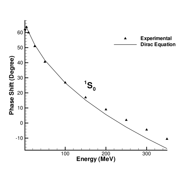
Figure 1: $np$ Scattering Phase Shift for ${}^{1}S_{0}$ State (Model 1)

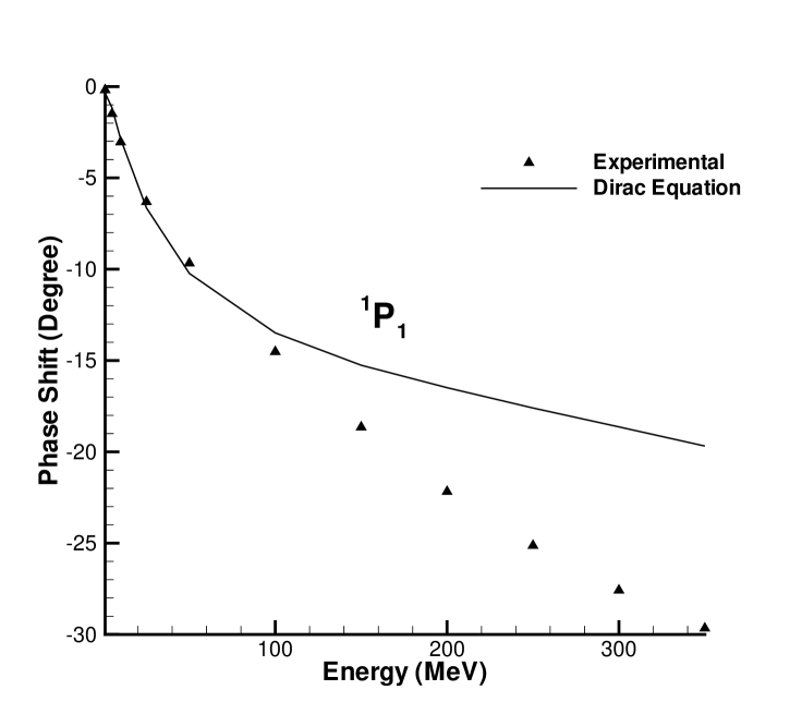
Figure 2: $np$ Scattering Phase Shift for ${}^{1}P_{1}$ State (Model 1)

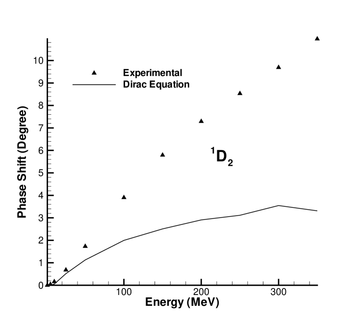
Figure 3: $np$ Scattering Phase Shift for ${}^{1}D_{2}$ State (Model 1)

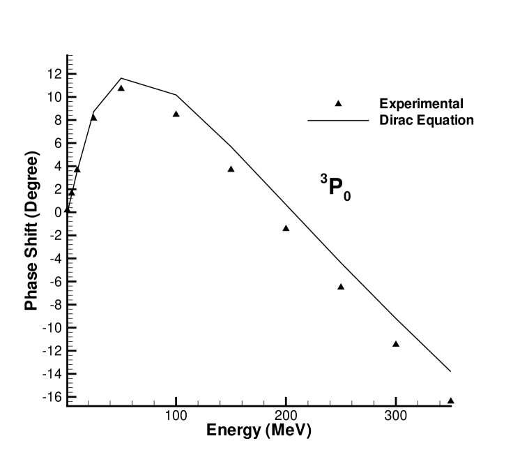
Figure 4: $np$ Scattering Phase Shift for ${}^{3}P_{0}$ State (Model 1)

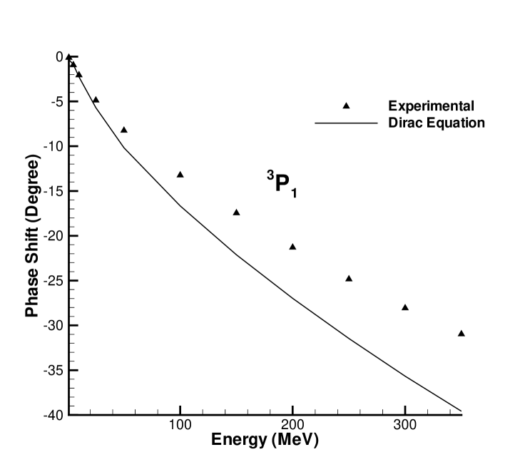
Figure 5: $np$ Scattering Phase Shift for ${}^{3}P_{1}$ State (Model 1)

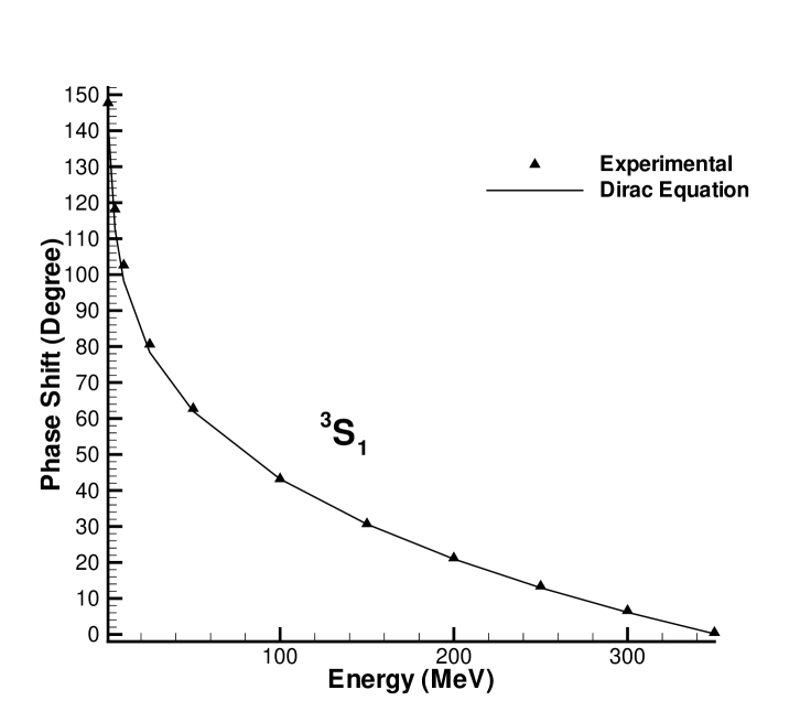
Figure 6: $np$ Scattering Phase Shift for ${}^{3}S_{1}$ State (Model 1)

Figure 7: $np$ Scattering Phase Shift for ${}^{3}D_{1}$ State (Model 1)

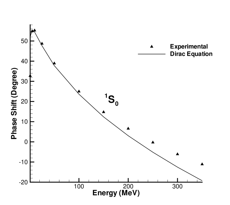
Figure 8: $pp$ Scattering Phase Shift for ${}^{1}S_{0}$ State (Model 1)

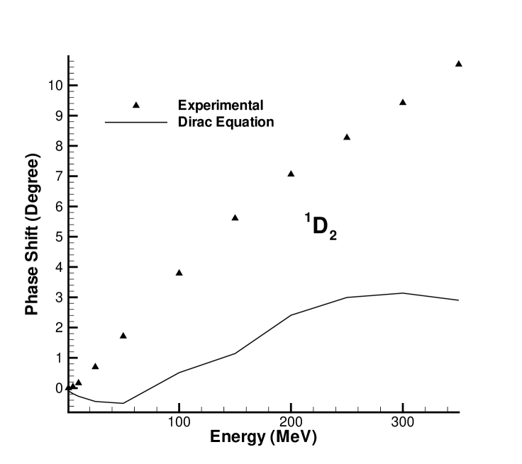
Figure 9: $np$ Scattering Phase Shift for ${}^{1}D_{2}$ State (Model 1)

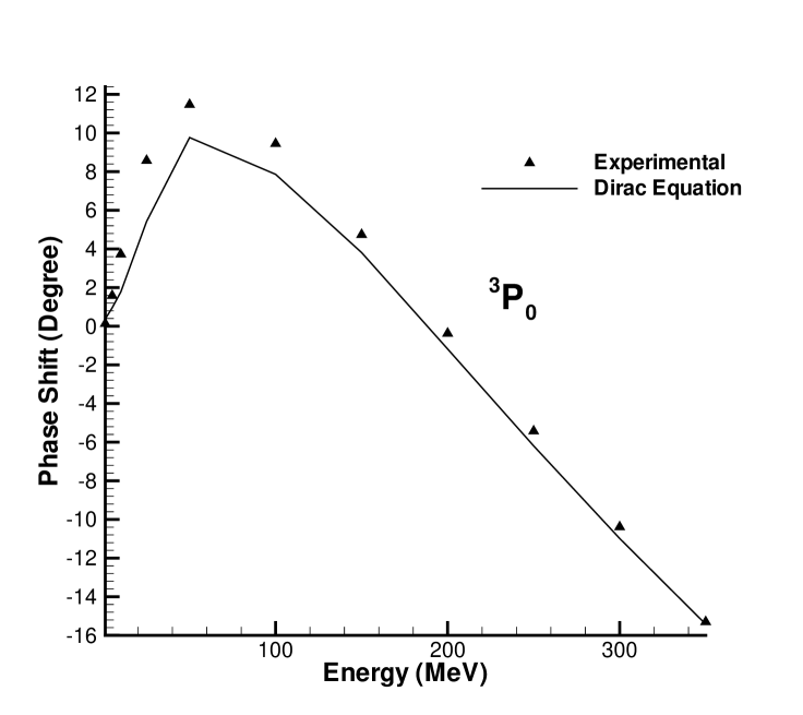
Figure 10: $pp$ Scattering Phase Shift for ${}^{3}P_{0}$ State (Model 1)

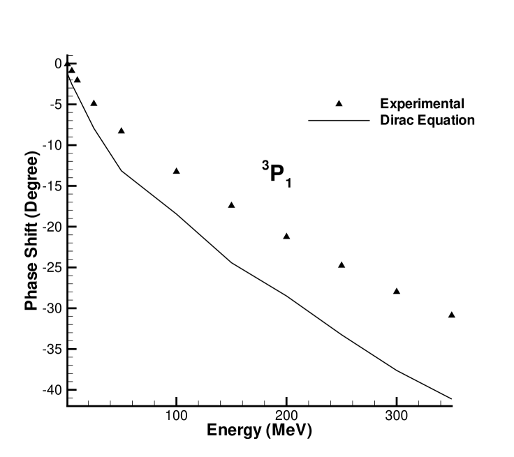
Figure 11: $pp$ Scattering Phase Shift for ${}^{3}P_{1}$ State (Model 1)

VI.2 Model 2

The theoretical phase shifts which we calculated by using the parameters for model 2 and the experimental phase shifts for all the seven states are listed in table 6. We also use the parameters for model 2 to predict the phase shift of $pp$ scattering.

Table 6: $np$ Scattering Phase Shift Of ${}^{1}S_{0}$, ${}^{1}P_{1}$, ${}^{1}D_{2}$, ${}^{3}P_{0}$, ${}^{3}P_{1}$, ${}^{3}S_{1}$ And ${}^{3}D_{1}$ States(Model 2).

Energy	${}^{1}S_{0}$	${}^{1}P_{1}$	${}^{1}D_{2}$	${}^{3}P_{0}$
(MeV)	Exp. The.	Exp. The.	Exp. The.	Exp. The.
1	62.07 60.60	-0.187 -0.358	0.00 0.02	0.18 0.00
5	63.63 63.50	-1.487 -1.163	0.04 0.15	1.63 1.61
10	59.96 60.20	-3.039 -2.857	0.16 0.39	3.65 3.74
25	50.90 51.44	-6.311 -6.629	0.68 0.40	8.13 9.28
50	40.54 40.91	-9.670 -10.36	1.73 1.37	10.70 12.69
100	26.78 25.86	-14.52 -14.44	3.90 2.42	8.460 11.74
150	16.94 14.62	-18.65 -17.55	5.79 3.62	3.690 7.399
200	8.940 5.435	-22.18 -20.37	7.29 4.55	-1.44 2.36
250	1.960 -2.428	-25.13 -23.15	8.53 5.24	-6.51 -2.78
300	-4.460 -9.330	-27.58 -25.87	9.69 5.34	-11.47 -7.746
350	-10.59 -15.52	-29.66 -28.54	10.96 5.30	-16.39 -12.52
Energy	${}^{3}P_{1}$	${}^{3}S_{1}$	${}^{3}D_{1}$	$\varepsilon$
(MeV)	Exp. The.	Exp. The.	Exp. The.	Exp. The.
1	-0.11 -0.32	147.747 144.797	-0.005 0.719	0.105 0.264
5	-0.94 -0.81	118.178 115.232	-0.183 -0.172	0.672 1.106
10	-2.06 -2.08	102.611 100.668	-0.677 -0.239	1.159 1.723
25	-4.88 -5.07	80.63 80.66	-2.799 -2.834	1.793 2.099
50	-8.25 -8.68	62.77 64.30	-6.433 -6.798	2.109 1.708
100	-13.24 -13.55	43.23 45.68	-12.23 -13.77	2.420 1.663
150	-17.46 -17.74	30.72 33.35	-16.48 -19.34	2.750 1.541
200	-21.30 -21.67	21.22 23.80	-19.71 -24.11	3.130 1.648
250	-24.84 -25.47	13.39 15.90	-22.21 -28.38	3.560 1.834
300	-28.07 -29.14	6.600 9.099	-24.14 -32.29	4.030 1.965
350	-30.97 -32.67	0.502 3.095	-25.57 -36.01	4.570 2.147

Table 7: $pp$ Scattering Phase Shift Of ${}^{1}S_{0}$, ${}^{1}D_{2}$, ${}^{3}P_{0}$ And ${}^{3}P_{1}$ States(Model 2).

Energy	${}^{1}S_{0}$	${}^{1}D_{2}$	${}^{3}P_{0}$	${}^{3}P_{1}$
MeV	Exp. The.	Exp. The.	Exp. The.	Exp. The.
1	32.68 52.40	0.001 -0.116	0.134 0.417	-0.081 -1.172
5	54.83 55.48	0.043 -0.232	1.582 1.042	-0.902 -2.434
10	55.22 54.24	0.165 -0.327	3.729 1.934	-2.060 -3.682
25	48.67 47.13	0.696 -0.524	8.575 5.943	-4.932 -7.355
50	38.90 37.04	1.711 -0.505	11.47 10.88	-8.317 -11.57
100	24.97 22.85	3.790 0.994	9.450 9.417	-13.26 -15.41
150	14.75 11.82	5.606 2.036	4.740 5.543	-17.43 -19.97
200	6.550 2.845	7.058 3.211	–0.370 0.495	-21.25 -23.23
250	-0.31 -4.86	8.270 3.648	-5.430 -4.589	-24.77 -27.28
300	-6.15 -11.72	9.420 3.956	-10.39 -9.516	-27.99 -31.05
350	-11.13 -17.85	10.69 4.014	-15.30 -14.13	-30.89 -34.22

The prediction for the four $pp$ scattering states are listed in table 7. The results of model 2 for $np$ scattering are given in figure 12 to figure 18 and for $pp$ scattering are from figure 19 to figure 22. Our results show for this model an improvement over those of model 1 especially for the the singlet $P$ and $D$ states.  However there is still much to be desired in the fit. One possible cause of this problem is that we did not include tensor and pseudovector interactions in our covariant potentials, limiting ourselves to scalar, vector and pseudoscalar. Another may be the ignoring of the pseudovector coupling of the pseudoscalar mesons to  the nucleon. Our results in $pp$ scattering show that if we obtain a good fit in $np$ scattering our predicted results in $pp$ scattering will also be good. This means that it is unnecessary to include $pp$ scattering in the our fit, we may use the parameters obtained in $np$ scattering to predict the results in $pp$ scattering. Overall our results are promising and indicate that the two-body Dirac equations of constraint dynamics together with the meson exchange model are suitable to construct semi-phenomenological potential models for nucleon-nucleon scattering.

Figure 12: $np$ Scattering Phase Shift of ${}^{1}S_{0}$ State (Model 2)

Figure 13: $np$ Scattering Phase Shift of ${}^{1}P_{1}$ State (Model 2)

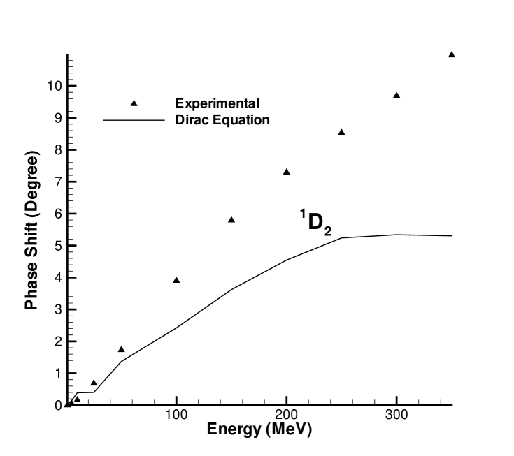
Figure 14: $np$ Scattering Phase Shift of ${}^{1}D_{2}$ State (Model 2)

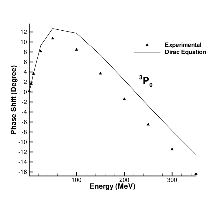
Figure 15: $np$ Scattering Phase Shift of ${}^{3}P_{0}$ State (Model 2)

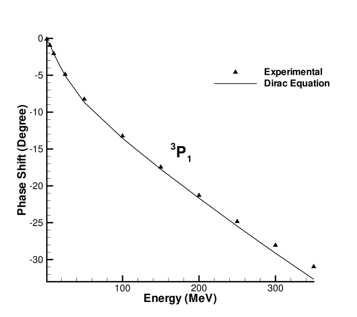
Figure 16: $np$ Scattering Phase Shift of ${}^{3}P_{1}$ State (Model 2)

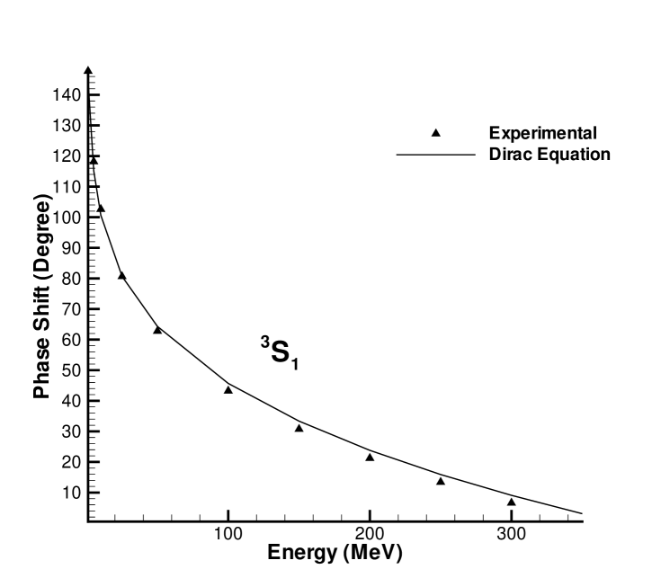
Figure 17: $np$ Scattering Phase Shift of ${}^{3}S_{1}$ State (Model 2)

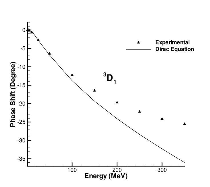
Figure 18: $np$ Scattering Phase Shift of ${}^{3}D_{1}$ State (Model 2)

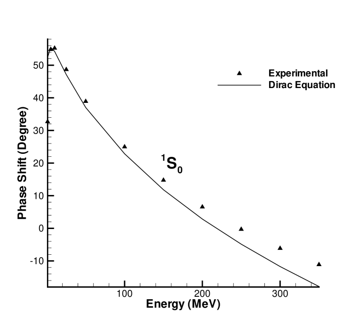
Figure 19: $pp$ Scattering Phase Shift of ${}^{1}S_{0}$ State (Model 2)

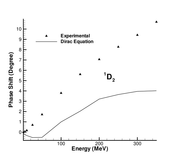
Figure 20: $pp$ Scattering Phase Shift of ${}^{1}D_{2}$ State (Model 2)

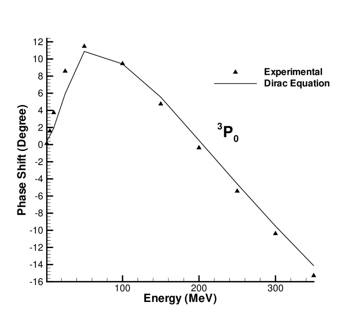
Figure 21: $pp$ Scattering Phase Shift of ${}^{3}P_{0}$ State (Model 2)

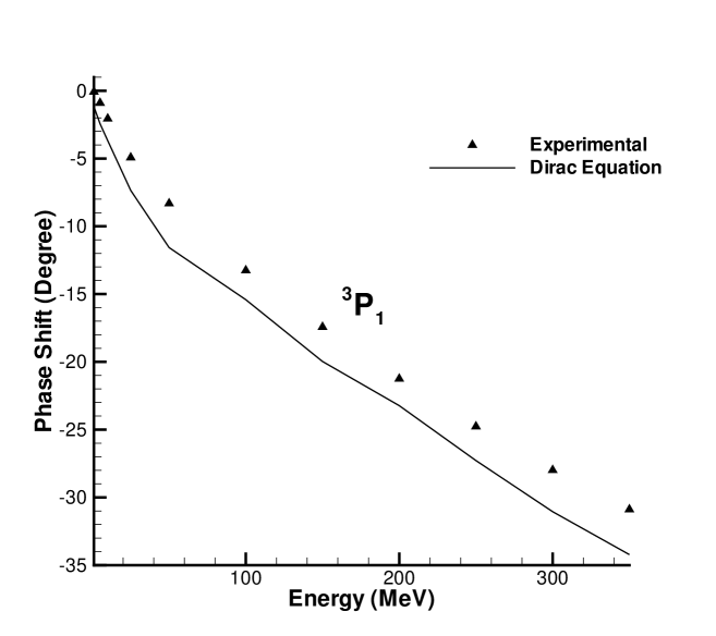
Figure 22: $pp$ Scattering Phase Shift of ${}^{3}P_{1}$ State (Model 2)

VII Conclusion

The two-body Dirac equations of constraint dynamics constitutes the first fully covariant treatment of the relativistic two-body problem that

a) includes constituent spin, b) regulates the relative time in a covariant manner, c) provides an exact reduction to 4 decoupled 4-component wave equations, d) includes non-perturbative recoil effects in a natural way that eliminates the need for singularity-softening parameters or finite particle size in semiphenomenological applications to QCD, e) is canonically equivalent in the semi-relativistic approximation to the Fermi-Breit approximation to the Bethe-Salpeter equation, f) unlike the Bethe-Salpeter equation and most other relativisitc approaches has a local momentum structure as simple as that of the nonrelativistic Schrödinger equation. g) is well-defined for zero-mass constituents (hence, permits investigation of the chiral symmetry limit) h) possesses spin structure that yields an exact solution for singlet positronium, i) has static limits that are relativistic, reducing to the ordinary single-particle Dirac equation in the limit that either particle becomes infinitely heavy. j) possesses a great variety of equivalent forms that are rearrangements of its two coupled Dirac equations (hence is directly related to many previously-known quantum descriptions of the relativistic two-body system).  These structures play an essential role in the success of this approach to both QCD and QED bound states. What is noteworthy in the latter appllication is that one need only identify the non-relativistic parts, i.e. the lowest order forms of $\mathcal{A}$ and $S$. The spin-dependent and covariant structure of the two-body Dirac formalism then automatically stamps out the correct semirelativistic spin dependent and spin independent corrections and provides well defined higher order relativistic corrections as well.  In addition the constraint formalism, although rooted in classical mechanics, has close connections to the Bethe-Salpeter equation of quantum field theory saz4 and with Wigner’s formulation of relativistic quantum mechanics as a symmetry of quantum theory plyz .

In this paper we have shown that these two-body Dirac equations may provide a reasonable account of the nucleon-nucleon scattering data when combined with the meson exchange model.  What makes this result important is that it is accomplished with a local and covariant formulation of the two-body problem.  What makes this unique is that this approach has been thoroughly tested in a nonperturbative context for both QED and QCD bound states. It is not a given that success in one or even both areas would imply that the formalism would do well in another.  In particular, the fits could have easily been disastrous given that the minimal coupling idea we have used (based in part on the earlier work on the quasipotential approach of Todorov).  The reason for some doubt is that these minimal coupling forms (generalized to the scalar interactions as well as the vector) lead to the scalar and vector potentials appearing squared.  Because of the size of the coupling constants, the deviation from the standard effective potentials could have been considerable in all cases. There are other nonperturbative structures that appear in the Pauli reduction of our equations to Schrödinger-like form (typical of what appears in the Pauli reduction of the one-body Dirac equation) that could also have prevented any reasonable results. So the general agreement we obtained with the data is very encouraging that this approach could be extended to include more general interactions.

An important step in our reduction was that we put the equation in a form for which we can apply the techniques which have been already developed for the Schrödinger-like system in nonrelativistic quantum mechanics.  This required that we get rid of first derivative terms. For the uncoupled states, it is pretty straightforward. For the coupled states we used a different spin-matirx approach that works for both the uncoupled and coupled states simultaneously.

We then tested several models by using the variable phase methods. We found it most  convenient to put all the angular momentum barrier terms in the potentials, and change all the phase shift equations to the form of $S$ state-like phase shift equations (see Eqs.(5.11,5.30,5.31,5.32)).

After several models and several methods to minimize our $\chi^{2}$ tested, we found two models which can lead us to a fairly good fit to the experimental phase shift data.

The most important equation used in our phase shift analysis for nucleon-nucleon scattering is Eq.(3.32) . It is a coupled Schrödinger-like equation derived from two-body Dirac equations with no approximations. All of our radial wave equations for any specific angular momentum state are obtained from this equation.

We use nine mesons in our fit. We summarize the meson-nucleon interactions we used by writing the quantum field theory Lagrange function for their effective interactions

$$L_{I} =g_{\sigma}\overline{\psi}\psi\sigma+g_{f_{0}}\overline{\psi}\psi f_{0}+g_{a_{0}}\overline{\psi}\mathbf{\tau}\psi\cdot\mathbf{a}_{0}$$

$$+g_{\rho}\overline{\psi}\gamma^{\mu}\mathbf{\tau}\psi\cdot\mathbf{\rho}_{\mu}+g_{\omega}\overline{\psi}\gamma^{\mu}\psi\omega_{\mu}+g_{\phi}\overline{\psi}\gamma^{\mu}\psi\phi_{\mu}$$

$$+g_{\pi}\overline{\psi}\gamma^{5}\mathbf{\tau}\psi\cdot\mathbf{\pi}+g_{\eta}\overline{\psi}\gamma^{5}\psi\eta+g_{\eta^{\prime}}\overline{\psi}\gamma^{5}\psi\eta^{\prime}$$ (7.1)

where $\psi$ represent the nucleon field, $\sigma$, $f_{0}$, … represent the meson fields.

Several models have been tested by using the variable phase methods, two models can lead us to a fairly good fit to the experimental phase shift data. We use the parameters which gives good fits to the $np$ scattering data to predict the phase shifts for the $pp$ scattering.  These lead to a good prediction for the $pp$ scattering based on the parameters we obtained (with noted exceptions). This means that our work has shown a promising result. The following are some suggestions to improve our work in the future.

VIII Suggestions For Future Work

VIII.1 Other Model Tests

More model testing is absolutely necessary in the future. By model we mean the way we place the perturbative interactions that arise from Eq.(7.1) into the nonperturbative forms we need for $L$, $C$ and $\mathcal{G}$. During our fits, we found that our final result are sensitive to the model we chose ranging from very bad fits to the fits presented here. Changing the way to modify the interactions and the way of mesons enter into the two-body Dirac equations may provide a new opportunity to improve our fit.

VIII.2 Including World Tensor Interactions

We have included just scalar, pseudoscalar and vector interactions in our potentials through the invariant forms like $L$, $C$ and $\mathcal{G}$. Treating two-body Dirac equations with tensor interactions of the vector meson may improve our fit. These tensor interacting were discussed earlier (see Eq.(4.16)) and correspond to non-minimal coupling of spin one-half particle not present in QED but which can not be ruled out in massive vector meson-nucleon interactions. The corresponding field theory interaction is

$$\Delta L_{I}=g_{\rho}^{\prime}\overline{\psi}\sigma^{\mu\nu}\mathbf{\tau}\psi\mathbf{\rho}_{\mu\nu}+g_{\omega}^{\prime}\overline{\psi}\sigma^{\mu\nu}\psi\omega_{\mu\nu}+g_{\phi}^{\prime}\overline{\psi}\sigma^{\mu\nu}\psi\phi_{\mu\nu}$$ (8.1)

and would correspond to relaxing the free field equation assumption made in Eq.(4.17)).

VIII.3 Include Pseudovector Interactions

Another option is to allow the pseudoscalar mesons($\pi$, $\eta$, and $\eta^{\prime}$) to interact with the nucleon not only by the pseudoscalar interaction(as in Eq.(7.1)) but also by the way of the pseudovector interactions as below

$$\Delta L_{I}=g_{\pi}^{\prime}\overline{\psi}\gamma^{\mu}\gamma^{5}\mathbf{\tau}\psi\partial_{\mu}\mathbf{\pi}+g_{\eta}^{\prime}\overline{\psi}\gamma^{\mu}\gamma^{5}\psi\partial_{\mu}\eta+g_{\eta^{\prime}}^{\prime}\overline{\psi}\gamma^{\mu}\gamma^{5}\psi\partial_{\mu}\eta^{\prime}$$ (8.2)

VIII.4 Include Full Massive Spin-One Propagator

We have ignored a portion of the massive spin-one propagator in our fit which is zero for particles on the mass shell. To include this portion of massive spin-one propagator we would have to change the vector propagator as below

$$\frac{\eta^{\mu\nu}}{q^{2}+m_{\rho}^{2}-i\varepsilon}\longrightarrow\frac{\eta^{\mu\nu}+\frac{q^{\mu}q^{\nu}}{m_{\rho}^{2}}}{q^{2}+m_{\rho}^{2}-i\varepsilon}.$$ (8.3)

Among all the four suggestions, the first one would be technically easiest once we finds models more general than the two we have presented here . The last three suggestions would involve corresponding additions to the interaction that appear in the two-body Dirac equations. Because the above interactions all involve derivative couplings we will  have to examine the CTBDE for the corresponding invariant $\Delta^{\prime}s$. These would include not only the eight invariants listed earlier (see Eq.(2.46) to Eq.(2.56)) but also four additional ones corresponding to $\Delta=R\theta_{1}\cdot\hat{x}_{\perp}\theta_{2}\cdot\hat{x}_{\perp},$ $~{}2S\theta_{51}\theta_{52}\theta_{1}\cdot\hat{x}_{\perp}\theta_{2}\cdot\hat{x}_{\perp}\ ,~{}$ $~{}2T\theta_{1}\cdot\hat{P}\theta_{1}\cdot\hat{P}\theta_{1}\cdot\hat{x}_{\perp}\theta_{2}\cdot\hat{x}_{\perp}$ and $4U\theta_{51}\theta_{52}\theta_{1}\cdot\hat{P}\theta_{1}\cdot\hat{P}\theta_{1}\cdot\hat{x}_{\perp}\theta_{2}\cdot\hat{x}_{\perp}.$  The four functions $R,S,T,U$ are each functions of $x_{\perp}$ and they represent space-like interactions paralleling those corresponding to $\mathcal{G},I,Y,$ and $\mathcal{F}$ respectively given earlier.  To include all 12 covariant matrix interactions will involve a significant modification of our basic equation Eq.(3.32) as well as the two-body Dirac equations given in Eqs(2.58,2.59).

VIII.5 Extentions to the N-Body Problem

Can the constraint formalism be extended to $N$-bodies?  There is no solution to the compatibility condition

$$[\mathcal{H}_{i},\mathcal{H}_{j}]|\psi\rangle=0;~{}~{}i,j=1,..,N$$ (8.4)

of generalized mass-shell constraints (or their Dirac counterparts) that has the simplicity of  the “third law” and tranversality conditions given in (2.14) and (2.15).  The difficulty involves satisfying Eq.(8.4) and cluster separability (needed to describe scattering states) at the same time.  Rohrlich has shown that this necessarily involves the introduction of $N-$body forces rohr . If one is willing to limit $N-$body considerations to bound states (so that cluster considerations are not important) then Ref. saz6 provides a constraint formalism in which a single dynamical wave equation (as in the two-body case) determines the bound state energies. Ref. luca (and references contained therein) provides an $N-$body constraint formalism that involves particles and fields leading in the end to directly inteacting particles by elimination of the field degrees of freedom by second class contraints.

Appendix A Pauli-Form of Two-Body Dirac Equations

We rewrite Eqs.(2.61,2.62) by multiplying the first by $\sqrt{2}i\beta_{1}$ and the second by $\sqrt{2}i\beta_{2}$ yielding long1

$$[T_{1}(\beta_{1}\beta_{2})+U_{1}(\beta_{1}\beta_{2})\gamma_{51}\gamma_{52}]|\psi\rangle=(E_{1}+M_{1}\beta_{1})\gamma_{51}|\psi\rangle$$

$$-[T_{2}(\beta_{1}\beta_{2})+U_{2}(\beta_{1}\beta_{2})\gamma_{51}\gamma_{52}]|\psi\rangle=(E_{2}+M_{2}\beta_{2})\gamma_{52}|\psi\rangle$$ (A.1)

in which the kinetic and recoil terms are

$$T_{1}(\beta_{1}\beta_{2})=\exp(\mathcal{G})[\mathbf{\Sigma}_{1}\cdot p-{\frac{i}{2}}\beta_{1}\beta_{2}(\mathbf{\Sigma}_{2}\cdot\partial(-C+\mathcal{G}\beta_{1}\beta_{2}\mathbf{\Sigma}_{1}\cdot\mathbf{\Sigma}_{2})]$$

$$T_{2}(\beta_{1}\beta_{2})=\exp(\mathcal{G})[\mathbf{\Sigma}_{2}\cdot p-{\frac{i}{2}}\beta_{1}\beta_{2}(\mathbf{\Sigma}_{1}\cdot\partial(-C+\mathcal{G}\beta_{1}\beta_{2}\mathbf{\Sigma}_{1}\cdot\mathbf{\Sigma}_{2})]$$ (A.2)

$$U_{1}(\beta_{1}\beta_{2})=\exp(\mathcal{G})[-{\frac{i}{2}}\beta_{1}\beta_{2}\mathbf{\Sigma}_{2}\cdot\partial(J\beta_{1}\beta_{2}-L)]$$

$$U_{2}(\beta_{1}\beta_{2})=\exp(\mathcal{G})[-{\frac{i}{2}}\beta_{1}\beta_{2}\mathbf{\Sigma}_{1}\cdot\partial(J\beta_{1}\beta_{2}-L)]$$ (A.3)

while the timelike and scalar potentials $E_{i},M_{i}$ are given above in Eqs.(2.63) and (2.64)

The final result of the matrix multiplication in Eqs.(A.1) is a set of eight simultaneous equations for the Dirac spinors $|\psi\rangle_{1},|\psi\rangle_{2},|\psi\rangle_{3},|\psi\rangle_{4}$. In an arbitrary frame, the result of the matrix calculation produces the eight simultaneous equations ($\sigma_{i}^{\mu}|\psi\rangle\rightarrow\Sigma_{i}^{\mu}|\psi\rangle_{1,2,3,4}$)long1 . One then reduces the eight equations to a second order Schrödinger-like equation by a process of substitution and elimination using the combinations of the four Dirac-spinors given below long1 :

$$|\phi_{\pm}\rangle\equiv|\psi\rangle_{1}\pm|\psi\rangle_{4},$$

$$|\chi_{\pm}\rangle\equiv|\psi\rangle_{2}\pm|\psi\rangle_{3}.$$ (A.4)

We display all the general spin dependent structures in $\Phi(\mathbf{r},\mathbf{p},{\mbox{\boldmath$\sigma$}}_{1},{\mbox{\boldmath$\sigma$}}_{2},w)$ explicitly, very similar to what appears in nonrelativistic formalisms such as seen in the Hamada-Johnson and Yale group models (as well as the nonrelativistic limit of Gross’s equation). We do this by expressing it explicitly in terms of its matrix (${\mbox{\boldmath$\sigma$}}_{1},{\mbox{\boldmath$\sigma$}}_{2}$), and operator $\mathbf{p}$ structure in the CM system ($\hat{P}=(1,\mathbf{0})$ ). We are working in the CM frame (i.e. $x_{\perp}=(\mathbf{r},0)$), so all the interaction functions ($L(x_{\perp}),J(x_{\perp}),C(x_{\perp}),\mathcal{G}(x_{\perp})$) are functions of $r=\sqrt{x_{\perp}^{2}}=\left|\mathbf{r}\right|$, $F=F(r)$

Ref. long1 finds the reduction

$$h[E_{1}[{\mbox{\boldmath$\sigma$}}_{1}\cdot\mathbf{p}-i{\mbox{\boldmath$\sigma$}}_{2}\cdot(\mathbf{d+k}{\mbox{\boldmath$\sigma$}}_{1}\cdot{\mbox{\boldmath$\sigma$}}_{2})]hF_{1}[{\mbox{\boldmath$\sigma$}}_{1}\cdot\mathbf{p}-i{{\mbox{\boldmath$\sigma$}}_{2}\cdot}(\mathbf{z+k}{\mbox{\boldmath$\sigma$}}_{1}\cdot{\mbox{\boldmath$\sigma$}}_{2})]|\phi_{+}\rangle\ \ \ \ \ \ \ \ \ \ \ \ \ \ \ \$$

$$+h[M_{1}[{\mbox{\boldmath$\sigma$}}_{1}\cdot\mathbf{p}-i{{\mbox{\boldmath$\sigma$}}_{2}\cdot}(\mathbf{o+k}{\mbox{\boldmath$\sigma$}}_{1}\cdot{\mbox{\boldmath$\sigma$}}_{2})]hF_{3}[{\mbox{\boldmath$\sigma$}}_{1}\cdot\mathbf{p}-i{{\mbox{\boldmath$\sigma$}}_{2}\cdot}(\mathbf{z+k}{\mbox{\boldmath$\sigma$}}_{1}\cdot{\mbox{\boldmath$\sigma$}}_{2})]|\phi_{+}\rangle\ \ \ \ \ \ \ \ \ \ \ \ \ \ \ \$$

$$-h[E_{1}[{\mbox{\boldmath$\sigma$}}_{1}\cdot\mathbf{p}-i{{\mbox{\boldmath$\sigma$}}_{2}\cdot}(\mathbf{d+k}{\mbox{\boldmath$\sigma$}}_{1}\cdot{\mbox{\boldmath$\sigma$}}_{2})]hF_{2}[{\mbox{\boldmath$\sigma$}}_{2}\cdot\mathbf{p}-i{{\mbox{\boldmath$\sigma$}}_{1}\cdot}(\mathbf{z+k}{\mbox{\boldmath$\sigma$}}_{1}\cdot{\mbox{\boldmath$\sigma$}}_{2})]|\phi_{+}\rangle\ \ \ \ \ \ \ \ \ \ \ \ \ \ \ \$$

$$+h[M_{1}[{\mbox{\boldmath$\sigma$}}_{1}\cdot\mathbf{p}-i{{\mbox{\boldmath$\sigma$}}_{2}\cdot}(\mathbf{o+k}{\mbox{\boldmath$\sigma$}}_{1}\cdot{\mbox{\boldmath$\sigma$}}_{2})]hF_{4}[{\mbox{\boldmath$\sigma$}}_{2}\cdot\mathbf{p}-i{{\mbox{\boldmath$\sigma$}}_{1}\cdot}(\mathbf{z+k}{\mbox{\boldmath$\sigma$}}_{1}\cdot{\mbox{\boldmath$\sigma$}}_{2})]|\phi_{+}\rangle\ \ \ \ \ \ \ \ \ \ \ \ \ \ \ \$$

$$=\mathcal{B}^{2}|\phi_{+}\rangle.$$ (A.5)

in which

$$\mathcal{B}^{2}=E_{1}{}^{2}-M_{1}{}^{2}=E_{2}{}^{2}-M_{2}{}^{2}$$

$$=b^{2}(w)+(\epsilon_{1}^{2}+\epsilon_{2}^{2})\mathrm{\sinh}^{2}(J)+2\epsilon_{1}\epsilon_{2}\sinh(J)\cosh(J)$$ (A.6)

$$-(m_{1}^{2}+m_{2}^{2})\mathrm{\sinh}^{2}(L)-2m_{1}m_{2}\sinh(L)\cosh(L).$$

and

$$h \equiv\exp(\mathcal{G}),\qquad$$

$$\mathbf{k} \equiv{\frac{1}{2}}\nabla\log(h),$$

$$\mathbf{z} \equiv{\frac{1}{2}}\nabla(-C+J-L)$$

$$\mathbf{d} \equiv{\frac{1}{2}}\nabla(C+J+L)$$

$$\mathbf{o} \equiv{\frac{1}{2}}\nabla(C-J-L).$$ (A.7)

with

$$F_{1}\equiv{\frac{M_{2}}{\mathcal{D}}}$$

$$F_{2}\equiv{\frac{M_{1}}{\mathcal{D}}}$$

$$F_{3}\equiv{\frac{E_{2}}{\mathcal{D}}}$$

$$F_{4}\equiv{\frac{E_{1}}{\mathcal{D}}}$$ (A.8)

$$\mathcal{D}\equiv E_{1}M_{2}+E_{2}M_{1}.$$ (A.9)

Eq.(A.5) is a second-order Schrödinger-like eigenvalue equation for the newly defined wavefunction $|\phi_{+}\rangle$ in the form.

$$(p_{\perp}^{2}+\Phi(r,\mbox{\boldmath$\sigma$}_{1},\mbox{\boldmath$\sigma$}_{2},w))|\phi_{+}\rangle=b^{2}(w)|\phi_{+}\rangle.$$ (A.10)

Eq.(3.5) for $\mathcal{B}^{2}$ provide us with the primary spin independent part of $\Phi$, the quasipotential. Note that in the CM system $p_{\perp}^{2}=\mathbf{p}^{2}$, $\sigma=(0,{\mbox{\boldmath$\sigma$}}).$For future reference we will refer to the four sets of terms on the left hand side as the Eq.(A.5) (a),(b),(c),(d) term.

Now we proceed with a different derivation than Long and Crater’s derivation long1 . The aim is to produce a Schrödinger like form like in Eq.(A.10) involving the Pauli matrices for both particles.

Substitute $\mathbf{d}$, $h$, $F_{1}$, $\mathbf{z}$, $\mathbf{k}$’s expressions to (a) term of Eq.(A.5), we obtain

$$\text{(a)\ \ term}=\exp(\mathcal{G})E_{1}\{[{\mbox{\boldmath$\sigma$}}_{1}\cdot\mathbf{p}-\frac{i}{2}{\mbox{\boldmath$\sigma$}}_{2}\cdot\nabla(C+J+L)-\frac{i}{2}\nabla\mathcal{G}\cdot({\mbox{\boldmath$\sigma$}}_{1}+i{\mbox{\boldmath$\sigma$}}_{1}\times{\mbox{\boldmath$\sigma$}}_{2})]$$

$$\times\exp(\mathcal{G}){\frac{M_{2}}{\mathcal{D}}[}{\mbox{\boldmath$\sigma$}}_{1}\cdot\mathbf{p}-\frac{i}{2}{\mbox{\boldmath$\sigma$}}_{2}\cdot\nabla(-C+J-L)-\frac{i}{2}\nabla\mathcal{G}\cdot({\mbox{\boldmath$\sigma$}}_{1}+i{\mbox{\boldmath$\sigma$}}_{1}\times{\mbox{\boldmath$\sigma$}}_{2})]\}$$ (A.11)

working out the commutation relation of ${\mbox{\boldmath$\sigma$}}_{1}\cdot\mathbf{p}$ in above expression, we can find the (a) term is

(a) term$=\exp(\mathcal{G})E_{1}\times$

$$\{\exp(\mathcal{G}){\frac{M_{2}}{\mathcal{D}}[\mathbf{p}}^{2}-\frac{i}{2}{\mbox{\boldmath$\sigma$}}_{2}\cdot\nabla(-C+J-L)({\mbox{\boldmath$\sigma$}}_{1}\cdot\mathbf{p})-\frac{i}{2}\nabla\mathcal{G}\cdot[(\mathbf{p}+i({\mbox{\boldmath$\sigma$}}_{1}\times\mathbf{p})-({\mbox{\boldmath$\sigma$}}_{1}\cdot{\mbox{\boldmath$\sigma$}}_{2})\mathbf{p}+{\mbox{\boldmath$\sigma$}}_{1}({\mbox{\boldmath$\sigma$}}_{2}\cdot\mathbf{p})-i({\mbox{\boldmath$\sigma$}}_{2}\times\mathbf{p})]]$$

$$+\frac{1}{i}{\mbox{\boldmath$\sigma$}}_{1}\cdot\partial[\exp(\mathcal{G}){\frac{M_{2}}{\mathcal{D}}[}{\mbox{\boldmath$\sigma$}}_{1}\cdot\mathbf{p}-\frac{i}{2}{\mbox{\boldmath$\sigma$}}_{2}\cdot\nabla(-C+J-L)-\frac{i}{2}\nabla\mathcal{G}\cdot({\mbox{\boldmath$\sigma$}}_{1}+i{\mbox{\boldmath$\sigma$}}_{1}\times{\mbox{\boldmath$\sigma$}}_{2})]]-$$

$$\frac{i}{2}[{\mbox{\boldmath$\sigma$}}_{2}\cdot\nabla(C+J+L)+\nabla\mathcal{G}\cdot({\mbox{\boldmath$\sigma$}}_{1}+i{\mbox{\boldmath$\sigma$}}_{1}\times{\mbox{\boldmath$\sigma$}}_{2})]\exp(\mathcal{G}){\frac{M_{2}}{\mathcal{D}}[}{\mbox{\boldmath$\sigma$}}_{1}\cdot\mathbf{p}-\frac{i}{2}{\mbox{\boldmath$\sigma$}}_{2}\cdot\nabla(-C+J-L)-\frac{i}{2}\nabla\mathcal{G}\cdot({\mbox{\boldmath$\sigma$}}_{1}+i{\mbox{\boldmath$\sigma$}}_{1}\times{\mbox{\boldmath$\sigma$}}_{2})]\}$$

Likewise we can the find (b),(c),(d) terms.

(b) term$=\exp(\mathcal{G})M_{1}\times$

$$\{\exp(\mathcal{G}){\frac{E_{2}}{\mathcal{D}}[\mathbf{p}}^{2}-\frac{i}{2}{\mbox{\boldmath$\sigma$}}_{2}\cdot\nabla(-C+J-L)({\mbox{\boldmath$\sigma$}}_{1}\cdot\mathbf{p})-\frac{i}{2}\nabla\mathcal{G}\cdot[(\mathbf{p}+i({\mbox{\boldmath$\sigma$}}_{1}\times\mathbf{p})-({\mbox{\boldmath$\sigma$}}_{1}\cdot{\mbox{\boldmath$\sigma$}}_{2})\mathbf{p}+{\mbox{\boldmath$\sigma$}}_{1}({\mbox{\boldmath$\sigma$}}_{2}\cdot\mathbf{p})-i({\mbox{\boldmath$\sigma$}}_{2}\times\mathbf{p})]]$$

$$+\frac{1}{i}{\mbox{\boldmath$\sigma$}}_{1}\cdot\partial[\exp(\mathcal{G}){\frac{E_{2}}{\mathcal{D}}[}{\mbox{\boldmath$\sigma$}}_{1}\cdot\mathbf{p}-\frac{i}{2}{\mbox{\boldmath$\sigma$}}_{2}\cdot\nabla(-C+J-L)-\frac{i}{2}\nabla\mathcal{G}\cdot({\mbox{\boldmath$\sigma$}}_{1}+i{\mbox{\boldmath$\sigma$}}_{1}\times{\mbox{\boldmath$\sigma$}}_{2})]]-$$

$$\frac{i}{2}[{\mbox{\boldmath$\sigma$}}_{2}\cdot\nabla(C-J-L)+\nabla\mathcal{G}\cdot({\mbox{\boldmath$\sigma$}}_{1}+i{\mbox{\boldmath$\sigma$}}_{1}\times{\mbox{\boldmath$\sigma$}}_{2})]\exp(\mathcal{G}){\frac{E_{2}}{\mathcal{D}}[}{\mbox{\boldmath$\sigma$}}_{1}\cdot\mathbf{p}-\frac{i}{2}{\mbox{\boldmath$\sigma$}}_{2}\cdot\nabla(-C+J-L)-\frac{i}{2}\nabla\mathcal{G}\cdot({\mbox{\boldmath$\sigma$}}_{1}+i{\mbox{\boldmath$\sigma$}}_{1}\times{\mbox{\boldmath$\sigma$}}_{2})]\}$$

(c) term$=-\exp(\mathcal{G})E_{1}\times$

$$\{\exp(\mathcal{G}){\frac{M_{1}}{\mathcal{D}}[}({\mbox{\boldmath$\sigma$}}_{2}\cdot\mathbf{p})({\mbox{\boldmath$\sigma$}}_{1}\cdot\mathbf{p})-\frac{i}{2}{\mbox{\boldmath$\sigma$}}_{1}\cdot\nabla(-C+J-L)({\mbox{\boldmath$\sigma$}}_{1}\cdot\mathbf{p})-\frac{i}{2}\nabla\mathcal{G}\cdot[({\mbox{\boldmath$\sigma$}}_{2}({\mbox{\boldmath$\sigma$}}_{1}\cdot\mathbf{p})-({\mbox{\boldmath$\sigma$}}_{1}\cdot{\mbox{\boldmath$\sigma$}}_{2})\mathbf{p}+{\mbox{\boldmath$\sigma$}}_{1}({\mbox{\boldmath$\sigma$}}_{2}\cdot\mathbf{p})$$

$$+i({\mbox{\boldmath$\sigma$}}_{2}\times\mathbf{p})]]+\frac{1}{i}{\mbox{\boldmath$\sigma$}}_{1}\cdot\partial[\exp(\mathcal{G}){\frac{M_{1}}{\mathcal{D}}[}{\mbox{\boldmath$\sigma$}}_{2}\cdot\mathbf{p}-\frac{i}{2}{\mbox{\boldmath$\sigma$}}_{1}\cdot\nabla(-C+J-L)-\frac{i}{2}\nabla\mathcal{G}\cdot({\mbox{\boldmath$\sigma$}}_{2}+i{\mbox{\boldmath$\sigma$}}_{2}\times{\mbox{\boldmath$\sigma$}}_{1})]]-$$

$$\frac{i}{2}[{\mbox{\boldmath$\sigma$}}_{2}\cdot\nabla(C+J+L)+\nabla\mathcal{G}\cdot({\mbox{\boldmath$\sigma$}}_{1}+i{\mbox{\boldmath$\sigma$}}_{1}\times{\mbox{\boldmath$\sigma$}}_{2})]\exp(\mathcal{G}){\frac{M_{1}}{\mathcal{D}}[}{\mbox{\boldmath$\sigma$}}_{2}\cdot\mathbf{p}-\frac{i}{2}{\mbox{\boldmath$\sigma$}}_{1}\cdot\nabla(-C+J-L)-\frac{i}{2}\nabla\mathcal{G}\cdot({\mbox{\boldmath$\sigma$}}_{2}+i{\mbox{\boldmath$\sigma$}}_{2}\times{\mbox{\boldmath$\sigma$}}_{1})]\}$$

(d) term$=\exp(\mathcal{G})M_{1}\times$

$$\{\exp(\mathcal{G}){\frac{E_{1}}{\mathcal{D}}[}({\mbox{\boldmath$\sigma$}}_{2}\cdot\mathbf{p})({\mbox{\boldmath$\sigma$}}_{1}\cdot\mathbf{p})-\frac{i}{2}{\mbox{\boldmath$\sigma$}}_{1}\cdot\nabla(-C+J-L)({\mbox{\boldmath$\sigma$}}_{1}\cdot\mathbf{p})-\frac{i}{2}\nabla\mathcal{G}\cdot[({\mbox{\boldmath$\sigma$}}_{2}({\mbox{\boldmath$\sigma$}}_{1}\cdot\mathbf{p})-({\mbox{\boldmath$\sigma$}}_{1}\cdot{\mbox{\boldmath$\sigma$}}_{2})\mathbf{p}+{\mbox{\boldmath$\sigma$}}_{1}({\mbox{\boldmath$\sigma$}}_{2}\cdot\mathbf{p})$$

$$+i({\mbox{\boldmath$\sigma$}}_{2}\times\mathbf{p})]]+\frac{1}{i}{\mbox{\boldmath$\sigma$}}_{1}\cdot\partial[\exp(\mathcal{G}){\frac{E_{1}}{\mathcal{D}}[}{\mbox{\boldmath$\sigma$}}_{2}\cdot\mathbf{p}-\frac{i}{2}{\mbox{\boldmath$\sigma$}}_{1}\cdot\nabla(-C+J-L)-\frac{i}{2}\nabla\mathcal{G}\cdot({\mbox{\boldmath$\sigma$}}_{2}+i{\mbox{\boldmath$\sigma$}}_{2}\times{\mbox{\boldmath$\sigma$}}_{1})]]-$$

$$\frac{i}{2}[{\mbox{\boldmath$\sigma$}}_{2}\cdot\nabla(C-J-L)+\nabla\mathcal{G}\cdot({\mbox{\boldmath$\sigma$}}_{1}+i{\mbox{\boldmath$\sigma$}}_{1}\times{\mbox{\boldmath$\sigma$}}_{2})]\exp(\mathcal{G}){\frac{E_{1}}{\mathcal{D}}[}{\mbox{\boldmath$\sigma$}}_{2}\cdot\mathbf{p}-\frac{i}{2}{\mbox{\boldmath$\sigma$}}_{1}\cdot\nabla(-C+J-L)-\frac{i}{2}\nabla\mathcal{G}\cdot({\mbox{\boldmath$\sigma$}}_{2}+i{\mbox{\boldmath$\sigma$}}_{2}\times{\mbox{\boldmath$\sigma$}}_{1})]\}$$

We simplify the above expressions by using identities involving ${\mbox{\boldmath$\sigma$}}_{1}$ and ${\mbox{\boldmath$\sigma$}}_{2}$ and group above equations by the $\mathbf{p}^{2}$ term , Darwin term $(\hat{\mathbf{r}}\cdot\mathbf{p)}$, spin-orbit angular momentum term $\mathbf{L}\cdot({\mbox{\boldmath$\sigma$}}_{1}+{\mbox{\boldmath$\sigma$}}_{2})$, spin-orbit angular momentum difference term $\mathbf{L}\cdot({\mbox{\boldmath$\sigma$}}_{1}-{\mbox{\boldmath$\sigma$}}_{2})$, spin-spin term $({\mbox{\boldmath$\sigma$}}_{1}\cdot{\mbox{\boldmath$\sigma$}}_{2})$, tensor term $({\mbox{\boldmath$\sigma$}}_{1}\cdot\hat{\mathbf{r}})({\mbox{\boldmath$\sigma$}}_{2}\cdot\hat{\mathbf{r}})$, additional spin dependent terms $\mathbf{L}\cdot({\mbox{\boldmath$\sigma$}}_{1}\times{\mbox{\boldmath$\sigma$}}_{2})$ and $({\mbox{\boldmath$\sigma$}}_{1}\cdot\hat{\mathbf{r}})({\mbox{\boldmath$\sigma$}}_{2}\cdot\mathbf{p})+({\mbox{\boldmath$\sigma$}}_{2}\cdot\hat{\mathbf{r}})({\mbox{\boldmath$\sigma$}}_{1}\cdot\mathbf{p}),$ and spin independent terms. Collecting all terms for the (a) + (b) + (c) + (d) terms our Eq.(A.5) becomes Eq.(3.4).

Appendix B Radial Equations   

The following are radial eigenvalue equations corresponding to Eq.(3.4) after getting rid of the first derivative terms for singlet states ${}^{1}S_{0}$, ${}^{1}P_{1}$, ${}^{1}D_{2}$( a general singlet ${}^{1}J_{j}$), triplet states ${}^{3}P_{1}$( a general let ${}^{3}J_{j}$), a general $s=1,$ $j=l+1$ ( ${}^{3}P_{0}$,${}^{3}S_{1}$ states $)$, and a general $s=1,$ $j=l+1$ $(^{3}D_{1}$ state).

${}^{1}S_{0}$, ${}^{1}P_{1}$, ${}^{1}D_{2}$ ( a general singlet ${}^{1}J_{j}$) $\mathbf{L}\cdot({\mbox{\boldmath$\sigma$}}_{1}+{\mbox{\boldmath$\sigma$}}_{2})=0$, ${\mbox{\boldmath$\sigma$}}_{1}\cdot{\mbox{\boldmath$\sigma$}}_{2}=-3$, ${\mbox{\boldmath$\sigma$}}_{1}\cdot\mathbf{\hat{r}}\mbox{\boldmath$\sigma$}_{2}\cdot\mathbf{\hat{r}=-}1.$

$$\{-\frac{d^{2}}{dr^{2}}+\frac{j(j+1)}{r^{2}}+\frac{g^{\prime 2}}{4}+h^{\prime 2}+\frac{g^{\prime\prime}}{2}+\frac{g^{\prime}}{r}\mathbf{-}3k-j-g^{\prime}h^{\prime}-h^{\prime\prime}-\frac{2h^{\prime}}{r}+m\}v=\mathcal{B}^{2}\exp(-2\mathcal{G})v$$ (B.1)

${}^{3}P_{1}$( a general triplet ${}^{3}J_{j}$) $\mathbf{L}\cdot({\mbox{\boldmath$\sigma$}}_{1}+{\mbox{\boldmath$\sigma$}}_{2})=-2$, ${\mbox{\boldmath$\sigma$}}_{1}\cdot{\mbox{\boldmath$\sigma$}}_{2}=1$, ${\mbox{\boldmath$\sigma$}}_{1}\cdot\mathbf{\hat{r}}\mbox{\boldmath$\sigma$}_{2}\cdot\mathbf{\hat{r}=}1.$

$$\{-\frac{d^{2}}{dr^{2}}+\frac{j(j+1)}{r^{2}}+\frac{g^{\prime 2}}{4}+h^{\prime 2}+\frac{g^{\prime\prime}}{2}+k+n+g^{\prime}h^{\prime}+h^{\prime\prime}+m\}v=\mathcal{B}^{2}\exp(-2\mathcal{G})v,$$ (B.2)

$s=1,$ $j=l+1$ ( ${}^{3}S_{1}$ states $)$

$\mathbf{L}\cdot({\mbox{\boldmath$\sigma$}}_{1}+{\mbox{\boldmath$\sigma$}}_{2})=2(j-1)$, ${\mbox{\boldmath$\sigma$}}_{1}\cdot{\mbox{\boldmath$\sigma$}}_{2}=1$, ${\mbox{\boldmath$\sigma$}}_{1}\cdot\mathbf{\hat{r}}\mbox{\boldmath$\sigma$}_{2}\cdot\mathbf{\hat{r}=}\frac{1}{2j+1}$ (diagonal term), and ${\mbox{\boldmath$\sigma$}}_{1}\cdot\mathbf{\hat{r}}\mbox{\boldmath$\sigma$}_{2}\cdot\mathbf{\hat{r}=}\frac{2\sqrt{j(j+1)}}{2j+1}$(off diagonal term).

$$\{-\frac{d^{2}}{dr^{2}}+\frac{j(j-1)}{r^{2}}{+}\frac{3g^{\prime}\sinh^{2}h}{r}+6h^{\prime}\frac{\cosh h\sinh h}{r}-\frac{6\sinh^{2}h}{r^{2}}-\frac{g^{\prime}\cosh h\sinh h}{r}$$

$$-2h^{\prime}\frac{\sinh^{2}h}{r}+2\frac{\cosh h\sinh h}{r^{2}}+\frac{g^{\prime 2}}{4}+h^{\prime 2}+\frac{g^{\prime\prime}}{2}+\frac{g^{\prime}}{r}+k$$

$$+2(j-1)[\frac{g^{\prime}}{2r}+\frac{g^{\prime}\sinh^{2}h}{r}-2\frac{\sinh^{2}h}{r^{2}}+2h^{\prime}\frac{\cosh h\sinh h}{r}]$$

$$+\frac{2(j-1)}{2j+1}[2h^{\prime}\frac{\sinh^{2}h}{r}-2\frac{\cosh h\sinh h}{r^{2}}+\frac{h^{\prime}}{r}+\frac{g^{\prime}\cosh h\sinh h}{r}]$$

$$+\frac{1}{2j+1}[\frac{3g^{\prime}\cosh h\sinh h}{r}-\frac{g^{\prime}\sinh^{2}h}{r}-2h^{\prime}\frac{\cosh h\sinh h}{r}+6h^{\prime}\frac{\sinh^{2}h}{r}$$

$$-6\frac{\cosh h\sinh h}{r^{2}}+2\frac{\sinh^{2}h}{r^{2}}+n+g^{\prime}h^{\prime}+h^{\prime\prime}+\frac{2h^{\prime}}{r}]+m\}u_{+}$$

$$+\frac{2\sqrt{j(j+1)}}{2j+1}\{\frac{3g^{\prime}\cosh h\sinh h}{r}-\frac{g^{\prime}\sinh^{2}h}{r}-2h^{\prime}\frac{\cosh h\sinh h}{r}+6h^{\prime}\frac{\sinh^{2}h}{r}$$

$$-6\frac{\cosh h\sinh h}{r^{2}}+2\frac{\sinh^{2}h}{r^{2}}+n+g^{\prime}h^{\prime}+h^{\prime\prime}+\frac{2h^{\prime}}{r}$$

$$+2(j-1)[\frac{2h^{\prime}\sinh^{2}(h)}{r}-\frac{2\cosh(h)\sinh(h)}{r^{2}}+\frac{h^{\prime}}{r}+\frac{g^{\prime}\cosh(h)\sinh(h)}{r}]\}u_{-}=\mathcal{B}^{2}\exp(-2\mathcal{G})u_{+},$$ (B.3)

$s=1,$ $j=l-1$ ( ${}^{3}P_{0}$,${}^{3}D_{1}$ states $)$

$\mathbf{L}\cdot({\mbox{\boldmath$\sigma$}}_{1}+{\mbox{\boldmath$\sigma$}}_{2})=-2(j+2)$, ${\mbox{\boldmath$\sigma$}}_{1}\cdot{\mbox{\boldmath$\sigma$}}_{2}=1$, ${\mbox{\boldmath$\sigma$}}_{1}\cdot\mathbf{\hat{r}}\mbox{\boldmath$\sigma$}_{2}\cdot\mathbf{\hat{r}=-}\frac{1}{2j+1}$(diagonal term), and ${\mbox{\boldmath$\sigma$}}_{1}\cdot\mathbf{\hat{r}}\mbox{\boldmath$\sigma$}_{2}\cdot\mathbf{\hat{r}=}\frac{2\sqrt{j(j+1)}}{2j+1}$(off diagonal term).

$$\{-\frac{d^{2}}{dr^{2}}+\frac{(j+1)(j+2)}{r^{2}}{+}\frac{3g^{\prime}\sinh^{2}h}{r}+6h^{\prime}\frac{\cosh h\sinh h}{r}-\frac{6\sinh^{2}h}{r^{2}}-\frac{g^{\prime}\cosh h\sinh h}{r}$$

$$-2h^{\prime}\frac{\sinh^{2}h}{r}+2\frac{\cosh h\sinh h}{r^{2}}+\frac{g^{\prime 2}}{4}+h^{\prime 2}+\frac{g^{\prime\prime}}{2}+\frac{g^{\prime}}{r}+k$$

$$+2(j+2)[\frac{g^{\prime}}{2r}+\frac{g^{\prime}\sinh^{2}h}{r}-2\frac{\sinh^{2}h}{r^{2}}+2h^{\prime}\frac{\cosh h\sinh h}{r}]$$

$$+\frac{2(j-1)}{2j+1}[2h^{\prime}\frac{\sinh^{2}h}{r}-2\frac{\cosh h\sinh h}{r^{2}}+\frac{h^{\prime}}{r}+\frac{g^{\prime}\cosh h\sinh h}{r}]$$

$$-\frac{1}{2j+1}[\frac{3g^{\prime}\cosh h\sinh h}{r}-\frac{g^{\prime}\sinh^{2}h}{r}-2h^{\prime}\frac{\cosh h\sinh h}{r}+6h^{\prime}\frac{\sinh^{2}h}{r}$$

$$-6\frac{\cosh h\sinh h}{r^{2}}+2\frac{\sinh^{2}h}{r^{2}}+n+g^{\prime}h^{\prime}+h^{\prime\prime}+\frac{2h^{\prime}}{r}]+m\}u_{-}$$

$$+\frac{2\sqrt{j(j+1)}}{2j+1}\{\frac{3g^{\prime}\cosh h\sinh h}{r}-\frac{g^{\prime}\sinh^{2}h}{r}-2h^{\prime}\frac{\cosh h\sinh h}{r}+6h^{\prime}\frac{\sinh^{2}h}{r}$$

$$-6\frac{\cosh h\sinh h}{r^{2}}+2\frac{\sinh^{2}h}{r^{2}}+n+g^{\prime}h^{\prime}+h^{\prime\prime}+\frac{2h^{\prime}}{r}$$

$$-2(j+2)[\frac{2h^{\prime}\sinh^{2}(h)}{r}-\frac{2\cosh(h)\sinh(h)}{r^{2}}+\frac{h^{\prime}}{r}+\frac{g^{\prime}\cosh(h)\sinh(h)}{r}]\}u_{+}=\mathcal{B}^{2}\exp(-2\mathcal{G})u_{-},$$ (B.4)

Substituting for $g^{\prime},h^{\prime},m,n,k$ we obtain the radial equations and potentials $\Phi$ given in the text.

Appendix C Derivation of Coupled Phase Shift Equations

We have found that we can use the Messiah ansatz quant .

$$u =A\sin(br+\delta)$$

$$u^{\prime} =bA\cos(br+\delta)$$ (C.1)

for the solution of

$$(-\frac{d^{2}}{dr^{2}}+\Phi_{L}(r))u=b^{2}u(r)$$ (C.2)

to yield

$$\delta^{\prime}=-\frac{\Phi_{L}}{b}\sin^{2}(br+\delta)$$ (C.3)

Next we see how this can be worked out in the case of coupled radial equations of the form

$$-\left(\begin{array}[c]{c}u_{-}\\ u_{+}\end{array}\right)^{\prime\prime}+\Phi_{L}\left(\begin{array}[c]{c}u_{-}\\ u_{+}\end{array}\right)=b^{2}\left(\begin{array}[c]{c}u_{-}\\ u_{+}\end{array}\right).$$ (C.4)

where $\Phi_{L}$ is a two by two matrix. This equation will have solutions that are $S-$wave dominant and $D-$wave dominant.  Form them together into a $2\times 2$ matrix $U$ so that the above equation becomes

$$-U^{\prime\prime}+\Phi_{L}U=b^{2}U.$$ (C.5)

Then take its transpose and add the two.  One obtains

$$-(U^{\prime\prime}+U^{\prime^{\prime}T})+(\Phi_{L}U+U^{T}\Phi_{L}^{T})=b^{2}(U+U^{T})$$ (C.6)

In analogy to the uncoupled case we assume

$$U=A(r)\sin(br+\mathcal{D(}r)\mathbb{)}$$ (C.7)

where

$$\mathcal{D} \mathbb{=}\delta(r)+\mathbf{D(r)}\cdot{\mbox{\boldmath$\sigma$}}$$ (C.8)

$$A \mathbb{=}a(r)+\mathbf{A(r)}\cdot{\mbox{\boldmath$\sigma$}.}$$

Let $R$ be a matrix that diagonalizes the phase shift matrix function $\mathcal{D}(r)$ to the form $\delta(r)+D(r)\sigma_{3},$

$$\tilde{U}\mathbf{=}RUR^{-1}=\tilde{A}\sin(br+\delta+D\sigma_{3})$$ (C.9)

where

$$\tilde{A}=RAR^{-1}$$ (C.10)

Continuing the analogy we let

$$U^{\prime}=bA\cos(br+\mathcal{D}\mathbb{)}.$$ (C.11)

Then

$$RU^{\prime}R^{-1} =b\tilde{A}\cos(br+\delta+D\sigma_{3})=R(R^{-1}\tilde{U}R)^{\prime}R^{-1}$$ (C.12)

$$=RR^{-1\prime}\tilde{A}\sin(br+\delta+D\sigma_{3})+\tilde{A}^{\prime}\sin(br+\delta+D\sigma_{3})$$

$$+\tilde{A}(b+\delta^{\prime}+D^{\prime}\sigma_{3})\cos(br+\delta+D\sigma_{3})+\tilde{A}\sin(br+\delta+D\sigma_{3})R^{\prime}R^{-1}$$

But $RR^{-1\prime}=-R^{\prime}R^{-1}$ so that we obtain the condition

$$\tilde{A}^{\prime}\sin(br+\delta+D\sigma_{3})+\tilde{A}(\delta^{\prime}+D^{\prime}\sigma_{3})\cos(br+\delta+D\sigma_{3})+[\tilde{A}\sin(br+\delta+D\sigma_{3}),R^{\prime}R^{-1}]_{-}=0.$$ (C.13)

In general we would take

$$\tilde{A} \equiv a+\tilde{A}_{3}\sigma_{3}+\mathbf{\tilde{A}}_{\perp}\cdot{\mbox{\boldmath$\sigma$}}$$ (C.14)

$$\equiv\tilde{A}_{||}+\mathbf{\tilde{A}}_{\perp}\cdot{\mbox{\boldmath$\sigma$}}$$

and decompose Eq.(C.13) and Eq.(C.6) into two sets of  four coupled equations.

Give $R$ the following general form:

$$R =\exp(i\varepsilon(r)\sigma_{2})\exp(\eta(r)\sigma_{1})$$

$$R^{-1} =\exp(-\eta\sigma_{1})\exp(-i\varepsilon\sigma_{2})$$

$$R^{\prime} =i\varepsilon^{\prime}\sigma_{2}\exp(i\varepsilon\sigma_{2})\exp(\eta\sigma_{1})+\exp(i\varepsilon\sigma_{2})\exp(\eta\sigma_{1})\eta^{\prime}\sigma_{1}$$

$$R^{\prime}R^{-1} =i\varepsilon^{\prime}\sigma_{2}+\exp(i\varepsilon\sigma_{2})\eta^{\prime}\sigma_{1}\exp(-i\varepsilon\sigma_{2})$$

$$=i\varepsilon^{\prime}\sigma_{2}+\eta^{\prime}\cos(2\varepsilon)\sigma_{1}+\eta^{\prime}\sin(2\varepsilon)\sigma_{3}$$ (C.15)

We consider the case in which $\Phi_{L}$ is a symmtric matrix and furthermore that as a result $\mathcal{D=D}^{T}.$  In that case our matrix is $R$ is orthogonal ($\eta=0$).

Next we examine the three terms of Eq.(C.6).  We assume that $\mathbf{\tilde{A}}_{\perp}$ is symmetric so that $\tilde{A}_{2}=0$ and

$$b^{2}R(U+U^{T})R^{-1} =b^{2}[(\tilde{A}_{||}+\mathbf{\tilde{A}}_{\perp}\cdot{\mbox{\boldmath$\sigma$})}\sin(br+\delta+D\sigma_{3})+\sin(br+\delta+D\sigma_{3})(\tilde{A}_{||}+\mathbf{\tilde{A}}_{\perp}\cdot{\mbox{\boldmath$\sigma$}}]\mathbf{)}$$

$$=b^{2}[2\tilde{A}_{||}\sin(br+\delta+D\sigma_{3})+2(\tilde{A}_{1}\sin(br+\delta)\cos D)\sigma_{1}]$$ (C.16)

and

$$R(\Phi U+U^{T}\Phi^{T})R^{-1}$$

$$=(\tilde{\Phi}_{||}+\mathbf{\tilde{\Phi}}_{\perp}{\cdot\mbox{\boldmath$\sigma$})}(\tilde{A}_{||}+\mathbf{\tilde{A}}_{\perp}\cdot{\mbox{\boldmath$\sigma$})}\sin(br+\delta+D\sigma_{3})+(\text{Transpose})$$

$$=(\tilde{\Phi}_{||}\tilde{A}_{||}+\mathbf{\tilde{\Phi}}_{\perp}\cdot\mathbf{\tilde{A}}_{\perp}\mathbf{)}\sin(br+\delta+D\sigma_{3})$$

$$+(\tilde{\Phi}_{||}\mathbf{\tilde{A}}_{\perp}\cdot{\mbox{\boldmath$\sigma$}}+\mathbf{\tilde{\Phi}}_{\perp}\cdot{\mbox{\boldmath$\sigma$}}\tilde{A}_{||}+i\mathbf{\tilde{\Phi}}_{\perp}\times\mathbf{\tilde{A}}_{\perp}\cdot{\mbox{\boldmath$\sigma$}})\sin(br+\delta+D\sigma_{3})$$

$$+\sin(br+\delta+D\sigma_{3})(\tilde{\Phi}_{||}\tilde{A}_{||}+\mathbf{\tilde{\Phi}}_{\perp}\cdot\mathbf{\tilde{A}}_{\perp}\mathbf{)}$$

$$+\sin(br+\delta+D\sigma_{3})(\mathbf{\tilde{A}}_{\perp}\cdot{\mbox{\boldmath$\sigma$}}\tilde{\Phi}_{||}+\tilde{A}_{||}\mathbf{\tilde{\Phi}}_{\perp}\cdot{\mbox{\boldmath$\sigma$}}+i\mathbf{\tilde{\Phi}}_{\perp}\times\mathbf{\tilde{A}}_{\perp}\cdot{\mbox{\boldmath$\sigma$}})$$ (C.17)

The term $\mathbf{\tilde{\Phi}}_{\perp}\times\mathbf{\tilde{A}}_{\perp}\cdot{\mbox{\boldmath$\sigma$}}$ is zero since $\tilde{A}_{2}=0=\tilde{\Phi}_{2}.$ The second derivative term is

$$R(U^{\prime\prime}+U^{\prime\prime T})R^{T}$$

$$=R(R^{T}\tilde{U}^{\prime}R)^{\prime}R^{-1}+(\text{Transpose})$$

$$=bR(R^{T}\tilde{A}\cos(br+\delta+D\sigma_{3})R)^{\prime}R^{T}+(\text{Transpose})$$

$$=b\{[\tilde{A}\cos(br+\delta+D\sigma_{3}),R^{\prime}R^{T}]_{-}+\tilde{A}^{\prime}\cos(br+\delta+D\sigma_{3})$$

$$-\tilde{A}(b+\delta^{\prime}+D^{\prime}\sigma_{3})\sin(br+\delta+D\sigma_{3})\}+(\text{Transpose})$$

$$=b\{i\varepsilon^{\prime}[(\tilde{A}_{||}+\mathbf{\tilde{A}}_{\perp}\cdot{\mbox{\boldmath$\sigma$})}\cos(br+\delta+D\sigma_{3}),\sigma_{2}]_{-}+(\tilde{A}_{||}^{\prime}+\mathbf{\tilde{A}}_{\perp}^{\prime}\cdot{\mbox{\boldmath$\sigma$})}\cos(br+\delta+D\sigma_{3})$$

$$-(\tilde{A}_{||}+\mathbf{\tilde{A}}_{\perp}\cdot{\mbox{\boldmath$\sigma$})}(b+\delta^{\prime}+D^{\prime}\sigma_{3})\sin(br+\delta+D\sigma_{3})\}+(\text{Transpose})$$ (C.18)

Using properties of the Pauli matrices and dividing Eq.(C.13) and Eq.(C.6) into $||$ and $\perp$ components we obtain the four equations

$$-\tilde{A}_{||}(\delta^{\prime}+D^{\prime}\sigma_{3})\sin(br+\delta+D\sigma_{3})$$

$$+\tilde{A}_{||}^{\prime}\cos(br+\delta+D\sigma_{3})-2b\varepsilon^{\prime}\sigma_{3}\tilde{A}_{1}\cos(br+\delta)\cos D$$

$$=\frac{1}{b}(\tilde{\Phi}_{||}\tilde{A}_{||}+\tilde{\Phi}_{1}\tilde{A}_{1}\mathbf{)}\sin(br+\delta+D\sigma_{3}),$$ (C.19)

$$\tilde{A}_{||}^{\prime}\sin(br+\delta+D\sigma_{3})+\tilde{A}_{||}(\delta^{\prime}+D^{\prime}\sigma_{3})\cos(br+\delta+D\sigma_{3})-2\varepsilon^{\prime}\sigma_{3}\tilde{A}_{1}\sin(br+\delta)\cos D$$

$$=0,$$ (C.20)

$$\cos(br+\delta)\cos D\tilde{A}_{1}^{\prime}-(\delta^{\prime}\sin(br+\delta)\cos D+D^{\prime}\cos(br+\delta)\sin D)\tilde{A}_{1}$$

$$+2\varepsilon^{\prime}(\tilde{A}_{3}\cos(br+\delta)\cos D-a\sin(br+\delta)\sin D)$$

$$=\frac{1}{b}[\phi\sin(br+\delta)\cos D\tilde{A}_{1}-\tilde{\Phi}_{3}\cos(br+\delta)\sin D\tilde{A}_{1}$$

$$+(a\sin(br+\delta)\cos D+\tilde{A}_{3}(\cos(br+\delta)\sin D)\tilde{\Phi}_{1}],$$ (C.21)

$$\tilde{A}_{1}^{\prime}\sin(br+\delta)\cos D+\tilde{A}_{1}(\delta^{\prime}\cos(br+\delta)\cos D-D^{\prime}\sin(br+\delta)\sin D)$$

$$+2\varepsilon^{\prime}(a\cos(br+\delta)\sin D+\tilde{A}_{3}\sin(br+\delta)\cos D)$$

$$=0.$$ (C.22)

Combining Eq.(C.19) and Eq.(C.20) we obtain

$$-\tilde{A}_{||}(\delta^{\prime}+D^{\prime}\sigma_{3})-2\varepsilon^{\prime}\tilde{A}_{1}\sin D\cos D$$

$$=\frac{1}{b}(\tilde{\Phi}_{||}\tilde{A}_{||}+\tilde{\Phi}_{1}\tilde{A}_{1}\mathbf{)}\sin^{2}(br+\delta+D\sigma_{3}).$$ (C.23)

Combining Eq.(C.21) and Eq.(C.22) gives

$$\tilde{A}_{1}\delta^{\prime}\csc(br+\delta)\cos D-2\varepsilon^{\prime}\csc(br+\delta)\sin D$$

$$=\frac{1}{b}[(\phi\sin(br+\delta)\cos D-\tilde{\Phi}_{3}\cos(br+\delta)\sin D)\tilde{A}_{1}$$

$$+(a\sin(br+\delta)\cos D+\tilde{A}_{3}(\cos(br+\delta)\sin D)\tilde{\Phi}_{1}].$$ (C.24)

Rewrite the above two equations as

$$\tilde{A}_{||}[(\delta^{\prime}+D^{\prime}\sigma_{3})+\frac{1}{b}\tilde{\Phi}_{||}\sin^{2}(br+\delta+D\sigma_{3})]$$

$$+\tilde{A}_{1}(2\varepsilon^{\prime}\sin D\cos D+\frac{1}{b}\tilde{\Phi}_{1}\sin^{2}(br+\delta+D\sigma_{3}))$$

$$=0,$$ (C.25)

$$\frac{1}{b}(a\sin(br+\delta)\cos D+\tilde{A}_{3}\cos(br+\delta)\sin D)\tilde{\Phi}_{1}+2\varepsilon^{\prime}a\csc(br+\delta)\sin D$$

$$+\tilde{A}_{1}[\frac{1}{b}(\phi\sin(br+\delta)\cos D-\tilde{\Phi}_{3}\cos(br+\delta)\sin D)-\delta^{\prime}\csc(br+\delta)\cos D]$$

$$=0.$$ (C.26)

The first of these two equations is actually two equations

$$a[\delta^{\prime}+\frac{1}{2b}\phi(1-\cos 2(br+\delta)\cos(2D))+\frac{1}{2b}\tilde{\Phi}_{3}\sin 2(br+\delta)\sin(2D)]$$

$$\tilde{A}_{3}[D^{\prime}+\frac{1}{2b}\tilde{\Phi}_{3}(1-\cos 2(br+\delta)\cos(2D))+\frac{1}{2b}\phi\sin 2(br+\delta)\sin(2D)]$$

$$+\tilde{A}_{1}((\varepsilon^{\prime}\sin 2D+\frac{1}{2b}\tilde{\Phi}_{1}(1-\cos 2(br+\delta)\cos 2D))$$

$$=0$$ (C.27)

and

$$a[D^{\prime}+\frac{1}{2b}\tilde{\Phi}_{3}(1-\cos 2(br+\delta)\cos(2D))+\frac{1}{2b}\phi\sin 2(br+\delta)\sin(2D)]$$

$$+\tilde{A}_{3}[\delta^{\prime}+\frac{1}{2b}\phi(1-\cos 2(br+\delta)\cos(2D))+\frac{1}{2b}\tilde{\Phi}_{3}\sin 2(br+\delta)\sin(2D)]$$

$$+\tilde{A}_{1}\frac{1}{2b}\tilde{\Phi}_{1}\sin 2(br+\delta)\sin 2D$$

$$=0.$$ (C.28)

So now together with Eq.(C.26)

$$a[\frac{1}{b}\sin(br+\delta)\cos(D)\tilde{\Phi}_{1}+2\varepsilon^{\prime}\csc(br+\delta)\sin D]$$

$$+\tilde{A}_{3}[\frac{1}{b}\cos(br+\delta)\sin(D)\tilde{\Phi}_{1}]$$

$$+\tilde{A}_{1}[\frac{1}{b}(\phi\sin(br+\delta)\cos D-\tilde{\Phi}_{3}\cos(br+\delta)\sin D)-\delta^{\prime}\csc(br+\delta)\cos D]$$

$$=0$$ (C.29)

we have three homogeneous equations in $a,\tilde{A}_{3},\tilde{A}_{1}$.  We simplify these equations further by assuming that $\tilde{A}_{1}=0.\$

$$=a[\delta^{\prime}+\frac{1}{2b}\phi(1-\cos 2(br+\delta)\cos(2D))+\frac{1}{2b}\tilde{\Phi}_{3}\sin 2(br+\delta)\sin(2D)]$$

$$\tilde{A}_{3}[D^{\prime}+\frac{1}{2b}\tilde{\Phi}_{3}(1-\cos 2(br+\delta)\cos(2D))+\frac{1}{2b}\phi\sin 2(br+\delta)\sin(2D)]$$

$$=0$$ (C.30)

$$=a[D^{\prime}+\frac{1}{2b}\tilde{\Phi}_{3}(1-\cos 2(br+\delta)\cos(2D))+\frac{1}{2b}\phi\sin 2(br+\delta)\sin(2D)]$$

$$+\tilde{A}_{3}[\delta^{\prime}+\frac{1}{2b}\phi(1-\cos 2(br+\delta)\cos(2D))+\frac{1}{2b}\tilde{\Phi}_{3}\sin 2(br+\delta)\sin(2D)]$$

$$=0$$ (C.31)

$$a[\frac{1}{b}\sin(br+\delta)\cos(D)\tilde{\Phi}_{1}+2\varepsilon^{\prime}\csc(br+\delta)\sin D]$$

$$+\tilde{A}_{3}[\frac{1}{b}\cos(br+\delta)\sin(D)\tilde{\Phi}_{1}]$$

$$=0$$ (C.32)

The solution we seek is

$$\delta^{\prime}+\frac{1}{2b}\phi(1-\cos 2(br+\delta)\cos(2D))+\frac{1}{2b}\tilde{\Phi}_{3}\sin 2(br+\delta)\sin(2D)=0$$ (C.33)

$$D^{\prime}+\frac{1}{2b}\tilde{\Phi}_{3}(1-\cos 2(br+\delta)\cos(2D))+\frac{1}{2b}\phi\sin 2(br+\delta)\sin(2D)=0.$$ (C.34)

Let

$$\delta =\frac{1}{2}(\delta_{1}+\delta_{2})$$

$$D =\frac{1}{2}(\delta_{1}-\delta_{2}),$$ (C.35)

and that leads to

$$\delta_{1}^{\prime}=-\frac{1}{b}(\phi+\tilde{\Phi}_{3})\sin^{2}(br+\delta_{1})$$ (C.36)

$$\delta_{2}^{\prime}=-\frac{1}{b}(\phi-\tilde{\Phi}_{3})\sin^{2}(br+\delta_{2})$$ (C.37)

Returning to Eq.(C.22) we find it reduces to

$$\tilde{A}_{3}=-a\cot(br+\delta)\tan D.$$ (C.38)

and combining that with Eq.(C.32) yields

$$[\frac{1}{b}\sin(br+\delta)\cos(D)\tilde{\Phi}_{1}+2\varepsilon^{\prime}\csc(br+\delta)\sin D]$$

$$-\cot(br+\delta)\tan D[\frac{1}{b}\cos(br+\delta)\sin(D)\tilde{\Phi}_{1}]$$

$$=0$$

so that

$$\varepsilon^{\prime} =\frac{1}{2b}\tilde{\Phi}_{1}(\tan D\cos^{2}(br+\delta)-\sin^{2}(br+\delta)\cot(D))$$

$$=\frac{1}{2\sin D\cos(D)b}\tilde{\Phi}_{1}(\sin^{2}D\cos^{2}(br+\delta)-\sin^{2}(br+\delta)\cos^{2}(D))$$

$$=\frac{1}{b\sin 2D}\tilde{\Phi}_{1}\sin(br+\delta+D)\sin(br+\delta-D)$$ (C.39)

From the definintion of $\tilde{\Phi}$ we see that

$$\left(\begin{array}[c]{cc}\cos\varepsilon&\sin\varepsilon\\ -\sin\varepsilon&\cos\varepsilon\end{array}\right)\left(\begin{array}[c]{cc}\Phi_{3}&\Phi_{1}\\ \Phi_{1}&-\Phi_{3}\end{array}\right)\left(\begin{array}[c]{cc}\cos\varepsilon&-\sin\varepsilon\\ \sin\varepsilon&\cos\varepsilon\end{array}\right)$$ (C.46)

$$=\left(\begin{array}[c]{cc}\Phi_{3}\cos 2\varepsilon+\Phi_{1}\sin 2\varepsilon&-\Phi_{3}\sin 2\varepsilon+\Phi_{1}\cos 2\varepsilon\\ -\Phi_{3}\sin 2\varepsilon+\Phi_{1}\cos 2\varepsilon&-\Phi_{3}\cos 2\varepsilon-\Phi_{1}\sin 2\varepsilon\end{array}\right)=\left(\begin{array}[c]{cc}\tilde{\Phi}_{3}&\tilde{\Phi}_{1}\\ \tilde{\Phi}_{1}&-\tilde{\Phi}_{3}\end{array}\right)$$ (C.51)

So from this and Eqs.(C.36) and Eq.(C.37) we obtain the phase shift equations Eqs.(5.30,5.31) given in the text while Eq.(C.39 ) gives us Eq.(5.32).

Appendix D
 Phase Shift Equation With The Coulomb Potential

We review here the necessary modification of our phase equations when we consider $pp$ scattering c6 ; cal . When we study $pp$ scattering, we must consider the influence of the Coulomb potential. The general form of the uncoupled Schrödinger-like equation with Coulomb potential is c6

$$\left[-\frac{d^{2}}{dr^{2}}+\frac{l(l+1)}{r^{2}}-\frac{2\epsilon_{w}\alpha}{r}+\Delta\Phi\right]u(r)=b^{2}u(r),$$ (D.1)

where $\Delta\Phi$ consists of the short range parts of the effective potential, $\alpha$ is the fine structure constant. (Compare the Coulomb term with the first term on the right hand sides of Eqs.(2.27,2.29)). Due to the long range behavior of the potential in above equation, the asymptotic behavior of the wave function is

$$u(r)\overset{r\rightarrow\infty}{\longrightarrow}const\cdot\sin(br-\eta\ln 2br+\Delta),$$ (D.2)

in which

$$\Delta=\delta_{l}+\sigma_{l}-\frac{l\pi}{2},$$ (D.3)

where $\sigma_{l}=\arg\Gamma(l+1+i\eta)$ is the Coulomb phase shift, here $\eta=-\frac{\epsilon_{w}\alpha}{b}.$

We describe here the variable phase method to calculate the phase shift with the Coulomb potential. Consider the two differential equations

$$u^{\prime\prime}+(b^{2}-W-\overline{W})u=0,$$ (D.4)

and

$$\overline{u}^{\prime\prime}+(b^{2}-\overline{W})\overline{u}=0,\hskip 14.45377pt\hskip 14.45377pti=1,2$$ (D.5)

in which $u(0)=\overline{u}_{1}(0)=0.$ Let

$$\overline{W}(r) =-\frac{2\epsilon_{w}\alpha}{r},$$ (D.6)

$$W(r) =\frac{l(l+1)}{r^{2}}+\Delta\Phi,$$

so that

$$\overline{u}_{1}(r)\overset{r\rightarrow\infty}{\longrightarrow}const\cdot\sin(br-\eta\ln 2br+\overline{\Delta}),$$

$$\overline{u}_{2}(r)\overset{r\rightarrow\infty}{\longrightarrow}const\cdot\cos(br-\eta\ln 2br+\overline{\Delta}),$$ (D.7)

where $\overline{\Delta}=$ $\sigma_{0}.$

Just as in the variable phase method, we obtain a nonlinear first order differential equation for the phase shift function $\delta_{l}(r)$ such that $\delta_{l}(\infty)=\delta_{l},$ and $\delta_{l}(0)=0.$ This is done by rewriting $u(r)$ as

$$u(r)=\alpha(r)[\cos\gamma(r)\overline{u}_{1}(r)+\sin\gamma(r)\overline{u}_{2}(r)]$$ (D.8)

so that

$$\Delta=\overline{\Delta}+\gamma(\infty).$$ (D.9)

Since we have rewritten $u(r)$ in two arbitrary functions, we are free to impose a condition on $u(r)$

$$u^{\prime}(r)=\alpha^{\prime}(r)[\cos\gamma(r)\overline{u}_{1}^{\prime}(r)+\sin\gamma(r)\overline{u}_{2}^{\prime}(r)].$$ (D.10)

Combining $u(r)$ and $u^{\prime}(r)$ leads to

$$\gamma(r)=-\tan^{-1}[\frac{u(r)\overline{u}_{1}^{\prime}(r)-u^{\prime}(r)\overline{u}_{1}(r)}{u(r)\overline{u}_{2}^{\prime}(r)-u^{\prime}(r)\overline{u}_{2}(r)}]$$ (D.11)

where $\gamma(0)=0$, and $\overline{u}_{1}(r)=F_{0}(\eta,br)$ and $\overline{u}_{2}(r)=G_{0}(\eta,br)$ are the two Coulomb wave functions. With the Wronskian $F_{0}G_{0}^{\prime}-$ $F_{0}^{\prime}G_{0}=b$, we obtain, by differentiating, the differential equation

$$\gamma^{\prime}(r)=-W(r)[\cos\gamma(r)F_{0}(\eta,br)+\sin\gamma(r)G_{0}(\eta,br)]^{2}/b.$$ (D.12)

Note that for

$$W(r)\overset{r\rightarrow 0}{\longrightarrow}\frac{\lambda(\lambda+1)}{r^{2}},\hskip 36.135pt\frac{\lambda(\lambda+1)}{r^{2}}=\frac{l(l+1)}{r^{2}}-\frac{\alpha^{2}}{r^{2}},$$

$$F_{0}(\eta,br)\overset{r\rightarrow 0}{\longrightarrow}C_{0}br,$$

$$G_{0}(\eta,br)\overset{r\rightarrow 0}{\longrightarrow}\frac{1}{C_{0}},$$ (D.13)

we obtain the relation

$$\gamma^{\prime}(0)=-\frac{C_{0}^{2}b\lambda}{\lambda(\lambda+1)}.$$ (D.14)

Letting

$$\gamma(r)=\beta(r)+\eta(r),$$ (D.15)

where $\beta(r)$ is defined as

$$\beta^{\prime}(r)=-\frac{l(l+1)}{r^{2}}[\cos\gamma(r)F_{0}(\eta,br)+\sin\gamma(r)G_{0}(\eta,br)]^{2}/b$$ (D.16)

$\beta(r)$ has the exact solution

$$\gamma(r)=-\tan^{-1}[\frac{F_{l}(\eta,br)F_{0}^{\prime}(\eta,br)-F_{l}^{\prime}(\eta,br)F_{0}(\eta,br)}{F_{l}(\eta,br)G_{0}^{\prime}(\eta,br)-F_{l}^{\prime}(\eta,br)G_{0}(\eta,br)}]$$ (D.17)

with $\beta(0)=0$ and $\beta^{\prime}(0)=-\frac{C_{0}^{2}bl}{l(l+1)}$ and $\beta(\infty)=\sigma_{l}-\frac{l\pi}{2}-\sigma_{0},$ lead to

$$\delta_{l}=\eta(\infty).$$ (D.18)

Thus , if we solve

$$\eta^{\prime}(r) =[-\frac{l(l+1)}{r^{2}}+\Delta\Phi][\cos(\beta(r)+\eta(r))F_{0}(\eta,br)+\sin(\beta(r)+\eta(r))G_{0}(\eta,br)]^{2}/b$$

$$+\frac{l(l+1)}{r^{2}}[\cos\beta(r)F_{0}(\eta,br)+\sin\beta(r)G_{0}(\eta,br)]^{2}/b$$ (D.19)

with the condition $\eta(0)=0$, we obtain the additional phase shift(above the Coulomb phase shift ) by integration to $\eta(\infty).$

There is no Coulomb scattering for the coupled triplet ${}^{3}S_{1}$ and ${}^{3}D_{1}$ states as a consideration of Pauli principal would show.

References

(1)This paper is based on the Ph.D. dissertation ”Two-Body Dirac
Equations and Nucleon-Nucleon Scattering Phase Shift Analysis” of Bin Liu, The
University of Tennessee (2001) -http://etd.utk.edu:/2001/LiuBin.pdf
(2)P. Van Alstine and H. W. Crater, J. Math. Phys. 23, 1997(1982)
(3)H. W. Crater, P. Van Alstine Ann. Phys. 148, 57(1983)
(4)H. W. Crater, P. Van Alstine Phys. Rev. Lett. 53, 1527(1984)
(5)H. W. Crater, P. Van Alstine Phys. Rev. D36 3007(1987)
(6)H. W. Crater, P. Van Alstine Phys. Rev. D37, 1982(1988)
(7)H. Sazdjian, Phys. Rev. D33, 3401(1988)
(8)P. Long and H. Crater, J. of Math. Phys. 39, 124 (1998)
(9)J. M. B. Kellogg, I. I. Rabi, N. F. Ramsey, Jr., and J. R.
Zacharias, Phys. Rev. 55, 318(1939) and Phys. Rev. 57, 677(1940)
(10)O. Chamberlain, E. Segre, RDD. D. Tripp, et al Phys. Rev.
105, 288(1957)
(11)H. P. Stapp, et al, Phys. Rev. 105, 302(1957)
(12)T. Hamada and I. D. Johnston, Nucl. Phys. 34, 382(1962)
(13)K. E. Lassila, M. H. Hull , et al Phys. Rev. 126, 881(1962)
(14)Roderick V. Reid Jr., Annals of Physics, Vol. 50, 411-448 (1968)
(15)K. E. Lassila, M. H. Hull , Jr., H. M. Ruppel, F. A. MacDonald and
G. Breit, Phys. Rev. 126(1962)881
(16)Variable Phase Approach to Potential Scattering. F. Calogero,
Academic Press, 1967
(17)A. Degasperis, Nuovo Cimento, Vol. XXXIV, N. 6 (1964).
(18)Franz Gross, Phys. Rev. D 10, 223(1974)
(19)Franz Gross, et al, Phys. Rev. C45, 2094(1992)
(20)V. G. J. Stoks, et al, Phys. Rev. C48, 792(1993)
(21)J.W. Negele and Erich Vogt (eds.) Advances in Nuclear Physics.-
R. Machleidt, - Chapter 2, The Meson Theory of Nuclear Forces and Nuclear
Structure- See also R. Machleidt, Phys. Rev. C63, 024001 (2001)
(22)H. W. Crater, R. L. Becker, C.Y. Wong and P. Van Alstine Phys.
Rev. D46 5117(1992)
(23)H. W. Crater, P. Van Alstine Found. of Phys. 24, 297(1994)
(24)H. Crater, P. Van Alstine, hep-ph/0208186 , submitted for
publication to Phys. Rev. D1.
(25)G. Breit, Phys. Rev. 34, 553(1929)
(26)G. Breit, Phys. Rev. 36, 383(1930)
(27)G. Breit, Phys. Rev. 39, 616(1932)
(28)P. A. M. Dirac , Proc. R. Soc. London A 117, 610(1928)
(29)H.A. Bethe and E. E. Salpeter, Quantum Mechanics of One
andTwo Electron Atoms (Springer, Berlin, 1957).
(30)H. W. Crater, C. W. Wong, and C. Y. Wong, Intl. J. Mod. Phys.
E 5, 589(1996)
(31)H. W. Crater, P. Van Alstine, Phys. Lett. 100B 166, (1981)
(32)H. W. Crater, P. Van Alstine, Phys. Rev. D30, 2585(1984)
(33)I. T. Todorov, in ” Properties of the
Fundamental Interactions”, ed by A. Zichichi, Vol. 9, Part C,
pp. 953-979; Phys. Rev. D3 2351(1971)
(34)P.A.M. Dirac, Lectures on Quantum Mechanics
(Yeshiva University, Hew York, 1964).
(35)H. W. Crater and P. Van Alstine, J. Math. Phys. 31, 1998(1990)
(36)H. Sazdjian has shown how the Bethe-Salpeter equation for two
particles may be algebraically transformed into the two generalized mass shell
constraints equations (2.9) and their spin-one half versions. H. Sazdjian
J. Math. Phys. 28, 2618 (1987), Extended Objects and Bound Systems,
Proc. of the Karuizawa International Symposium, 1992, edited by O. Hara, S.
Ishida and S. Naka (World Scientific, Singapore, 1992), p. 117.
(37)C. Y. Wong, H. Crater, Phys. Rev C63 044907 (2001) ( nucl-th/0010003)
(38)J. Mourad, H. Sazdjian, J. of Phys. G 21, 267(1995)
(39)H. W. Crater and D. Yang, J. Math. Phys. 32, 2374(1991)
(40)H. W. Crater and P. Van Alstine, Phys. Rev. D46. 766(1992)
(41)H. Jallouli and H. Sazdjian, Annals of Physics, 253
,376 (1997)
(42)E. Wigner, Ann. Math. 40, 149 1939
(43)W. N. Polyzou, Phys. Rev. 32, 995 (1985)
(44)Since the CTBDE are the counterparts of the one-body Dirac
equation with eliminated field they possess an analogous inherited dynamical
“gauge invariance” with Eq.(2.65)
and Eq.(2.66) invariant under any gauge transformation of the form
(
is the phase change of the wave function).
(45)Review of Particle Physics, D. E. Groom et al., The European
Physical Journal C15 (2000) 1.
(47)See and in Eq.(3.43) and
and in Eq.(3.45). Here we let . Strictly speaking to
accommodate nonsymmetric potentials the variables phase method must be
modified. A possible route to this is indicated in Appendix C. In our
present case and we take .
(48)R. Koch and E. Pietarinen, Nucl. Phys. A336, 331(1980)
(49)R. A. Arndt, Z. Li, Phys. Rev. Lett. 65, 157(1990);R.
A. Arndt and R. L. Workman, Phys. Rev. C43, 2436(1991)
(50)J. Bergervoet, et al., Phys. Rev. Lett. 59,
2255(1987). J. Bergervoet, et al., Phys. Rev. C41, 1435(1990)
(51)J. J. Sakurai, Modern Quantum Mechanics, 1994 by Addison-Wesley
Publishing Company, ISBN 0-201-53929-2.
(52)F. Rohrlich, Phys. Rev. D23 , 1305 (1981)
(53)H. Sazdjian, Ann. Phys. 191, 52 (1989)
(54)H. Crater and L. Lusanna, Ann. Phys. 289, 87 (2001)