Self-Consistent Quasi-Particle RPA for the Description of Superfluid Fermi Systems.

Abstract

Self-Consistent Quasi-Particle RPA (SCQRPA) is for the first time applied to a more level pairing case. Various filling situations and values for the coupling constant are considered. Very encouraging results in comparison with the exact solution of the model are obtained. The nature of the low lying mode in SCQRPA is identified. The strong reduction of the number fluctuation in SCQRPA vs BCS is pointed out. The transition from superfluidity to the normal fluid case is carefully investigated.

I Introduction

One of the most spectacular quantum phenomena is the transition to the supraconducting or superfluid state in interacting Fermi systems. This happens e.g. in metals, liquid ${}^{3}He$, neutron stars, in finite nuclei, and it is actively searched for in systems of magnetically trapped atomic Fermions. In most of these systems the canonical mean field approach of Bardeen, Cooper, and Schrieffer (BCS) with a couple of adjustable parameters works astonishingly well. However, in recent years there have been increasing attempts to describe the pairing phenomenon on completely microscopic grounds. To our knowledge these attempts have mostly been carried out for nuclear systems. This stems on the one hand from the fact that phenomenological $NN$ forces are on the market which very well describe the nucleon-nucleon phase shifts in all channels and in a wide range of energies. On the other hand the physics of neutron stars makes quantitative predictions of the pairing phenomenon in neutron matter indispensable, since superfluidity of neutrons stars manifests itself only quite indirectly through e.g. the phenomenon of neutron star glitches. The microscopic approaches to pairing, starting from a bare two body interaction, are not very numerous. The simplest one is based on BCS theory, using however, in the gap equation the bare force and for the single particle dispersion the one given by Brückner theory. In this way one obtains e.g. gap values in the ${}^{1}S_{0}$ channel for neutron-neutron pairing which in infinite matter, as a function of the Fermi momentum $k_{F}$, have a typical bell shaped form roughly dropping to zero around $k_{F}=1.3fm^{-1}$ and culminating at $k_{F}=0.8fm^{-1}$ to values of $\Delta=2.5-3.0MeV$ for neutron and nuclear matter respectively. This rather elementary approach has been extended in the past in various ways. The most ambitious procedure is probably the so-called correlated basis function approach b1 . However, more recently self-consistent T-matrix approaches and extended Brückner theories with rearrangement terms have achieved a remarkable degree of sophistication b2 . The screening of the interaction was treated to lowest order in the density, resuming the RPA bubbles, in introducing self-consistent Landau parameters b3 . The outcome of all these investigations inevitably leads to a quite substantial reduction of pairing in neutron matter but also in symmetric nuclear matter. The global reduction generally attains important values and often reaches factors close to three. Such small values of the gap in infinite matter, however, pose a problem. Employing the Local Density Approximation (LDA) to estimate from the infinite matter results the gap in finite nuclei b4 , one reaches with the simplified approach described above using the bare NN force quite reasonable gap values for finite nuclei. Interestingly in the gap equation quite similar results are obtained with the Gogny D${1}$S force b5 using the same procedure. However, with such strongly reduced gaps from the more sophisticated approaches mentioned above, one obtains much too small gaps in finite nuclei. Of course, this reasoning may be completely erroneous and the situation in finite nuclei may be very different from infinite matter. Nevertheless we find the above argumentation intriguing. On the other hand we know that pairing is an extraordinarily subtle process and employing theories which are in one or the other way uncontrolled may turn out to be a hazardous enterprise. In such a situation it is probably wise to investigate the problem from different sides using a variety of approaches.

In the past we have made very positive experience with an extension of RPA theory which we called Self-Consistent RPA (SCRPA) b6 ; b8 ; b7 . For instance, in a recent work this theory has been applied to the exactly solvable many level pairing model in the pre-critical regime and very good agreement with the exact results for ground-state energy and the low lying part of the spectrum was found b8 ; b7 . This success has encouraged us to develop the SCRPA formalism also for the fully developed superfluid regime. This is a not completely trivial extension of the SCRPA and we here apply it for the first time to the two level pairing model. As we will see the theory also gives very promising results in the superfluid phase. Since the Self-Consistent Quasi-Particle RPA (SCQRPA), as in general the SCRPA theory, can be derived from a variational principle, which turns out to be very close to a Raleigh-Ritz variational theory, we believe that SCQRPA is a non perturbative approach going in a certain systematic way beyond the mean field BCS theory, including in a self-consistent way correlations and quantum fluctuations. It is our believe that this microscopic approach can ultimately be used to calculate pairing properties of realistic Fermi systems starting from the bare force.

It should be mentioned that extensions of RPA theory, based on the Equation of Motion (EOM) method, have by now a quite long history. They, to a great deal, have been developed in nuclear physics. It started out with the work of Hara who included the ground-state correlation in the Fermion occupation numbers b9 . More systematic was the consequent work by Rowe and co-workers (see the review by D. J. Rowe c9 ). The same theory was developed using the Green’s function method by one of the present authors b6 . Independently the method was also proposed by Zimmermann and G. Röpke plus coworkers using a graphical construction b10 . These authors named their method Cluster-Hartree-Fock (CHF) and it is equivalent to Self-Consistent RPA (SCRPA). The latter approach has recently been further developed by Dukelsky and Schuck in a series of papers b8 ; b7 ; b15 ; b11 ; b12 ; b13 . However, also other authors contributed actively to the subject b14 . A number of remarkable results have been obtained with SCRPA in non trivial models where comparison with exact solutions was possible b7 ; b15 . For instance for the exactly solvable many level pairing model of Richardson b16 SCRPA provides very accurate results for the ground state and the low lying part of the spectrum b7 ; b8 .

In detail our paper is organized as follows : in section II the two level pairing model is introduced, in section III the SCQRPA formalism is presented, in section IV numerical results are given and detailed discussions are presented. Comparison with other recent works is made in section V, in section VI the question of the second constraint on the particle number variance is invoked and applied to the Seniority model. In section VII, we will summarize the results and draw some conclusions. Finally, some useful mathematical relations and a second method for the calculation of occupation numbers are given in the Appendices.

II The Model

The two-level pairing model is an exactly solvable model extensively employed in nuclear physics to test many-body approximations. It was first used to test the pp-RPA c24 and its ability to describe ground-state correlations and vibrations in the normal phase as well as in the superfluid phase. The model is composed of two levels with equal degeneracy $2\Omega=2J+1$ ($J$ is the spin of each level) and an single-particle energy splitting $\epsilon$. The pairing Hamiltonian in this model space is

$$H=\frac{\epsilon}{2}\sum_{j}j\hat{N}_{j}-g\Omega\sum_{j{j}^{\prime}}A_{j}^{\dagger}A_{{j}^{\prime}},\;j=\pm 1$$ (1)

where ${j}$ takes the values $1$ for the upper level and $-1$ for the lower level. $\hat{N}_{j}$ and $A^{\dagger}_{j}$ are the number and monopole pair operators of the level $j$, respectively,

$$A^{\dagger}_{j}=\frac{1}{\sqrt{\Omega}}\sum_{m=1}^{\Omega}a^{\dagger}_{jm}a^{\dagger}_{j\bar{m}}$$ (2)

and

$$\hat{N}_{j}=\sum_{m=1}^{\Omega}(a^{\dagger}_{jm}a_{jm}+a^{\dagger}_{j\bar{m}}a_{j\bar{m}}).$$ (3)

where $a^{\dagger}_{jm}$ creates a particle in the level $j$ with spin projection $m$ and $a_{j\bar{m}}=(-1)^{J-m}a_{j-m}$. The operators obey the following commutations relations,

$$[A_{j},A^{\dagger}_{j^{\prime}}] = \delta_{jj^{\prime}}\bigg{(}1-\frac{\hat{N}_{j}}{\Omega}\bigg{)},$$ (4)

$$[\hat{N}_{j},A^{\dagger}_{j^{\prime}}] = \delta_{jj^{\prime}}2A^{\dagger}_{j},$$ (5)

$$[\hat{N}_{j},A_{j^{\prime}}] = -\delta_{jj^{\prime}}2A_{j},$$ (6)

thus, they define an $SU(2)$ algebra for each level and the two level model satisfies an $SU(2)\times SU(2)$ algebra.

For a system not at half filling, the normalized states in the Hilbert subspace of the monopole pairs are

$$|n\rangle=\frac{{\Omega}^{\frac{\tilde{\Omega}}{2}}}{\Omega!}\sqrt{\frac{(\Omega-\tilde{\Omega}+n)!(\Omega-n)!}{n!(\tilde{\Omega}-n)!}}(A^{\dagger}_{1})^{n}(A^{\dagger}_{-1})^{\tilde{\Omega}-n}|0\rangle,\quad 0\leqslant n\leqslant\tilde{\Omega}$$ (7)

where $\tilde{\Omega}=\Omega$ leads to the half filling case, i.e. the lower level is filled for $g=0$. The matrix Hamiltonian is tridiagonal of dimension $\tilde{\Omega}+1$, with matrix elements

$$h_{n,n}=\langle n|H|n\rangle=\epsilon(2n-\tilde{\Omega})-G(2n\tilde{\Omega}-2n^{2}+\tilde{\Omega}\Omega-\tilde{\Omega}^{2}+\tilde{\Omega}),$$ (8)

$$h_{n-1,n}=\langle n-1|H|n\rangle=-G\sqrt{n(\Omega-(n-1))(\Omega-\tilde{\Omega}+n)(\tilde{\Omega}-n+1)}$$ (9)

where, $n$ is the number of pairs in the upper level and the number of particle is given by $N=2\tilde{\Omega}$.

III Self-consistent QRPA

In a recent work b7 the SCRPA has been applied with very good success to the picket fence model in the non superfluid phase. The extension to the superfluid phase is slightly delicate and we here limit ourselves to the two level model, however considering arbitrary degeneracies and fillings of the levels. The objective in this section is to establish the equations for the Self-Consistent Quasi-Particle RPA (SCQRPA). A first application of SCQRPA has been performed in b12 for the case of the seniority model (one-level pairing model). We will again later come back to this model. Here we want to consider the two level pairing model with arbitrary filling and coupling strength in the SCQRPA approach which already more or less shows the full complexity of more realistic many level problems. As a first step we have to transform the constrained Hamiltonian

$$H^{\prime}=H-\mu\hat{N},$$ (10)

where $\hat{N}$ is the full particle number operator, to quasi-particle operators

$$\pmatrix{\alpha^{\dagger}_{jm}\cr\alpha_{j\bar{m}}}=\pmatrix{u_{j}&-v_{j}\cr v_{j}&u_{j}}\pmatrix{a_{jm}^{\dagger}\cr a_{j\bar{m}}}$$ (11)

$$\pmatrix{a_{jm}^{\dagger}\cr a_{j\bar{m}}}=\pmatrix{u_{j}&v_{j}\cr-v_{j}&u_{j}}\pmatrix{\alpha^{\dagger}_{jm}\cr\alpha_{j\bar{m}}}$$ (12)

with

$$u_{j}^{2}+v_{j}^{2}=1,\;j=\pm 1.$$ (13)

We define new quasi spin operators as

$$P^{\dagger}_{j}=\frac{1}{\sqrt{\Omega}}\sum_{m>0}\alpha^{\dagger}_{jm}\alpha^{\dagger}_{j\bar{m}},\quad P_{j}=(P_{j}^{\dagger})^{\dagger}$$ (14)

and the quasi-particle number operator in the level $j$ is given by,

$$\hat{N}_{q,j}=\sum_{m>0}(\alpha^{\dagger}_{jm}\alpha_{jm}+\alpha^{\dagger}_{j\bar{m}}\alpha_{j\bar{m}}).$$ (15)

The quasi-particle operators obey the following commutations relations,

$$[P_{j},P^{\dagger}_{j^{\prime}}] = \delta_{jj^{\prime}}\bigg{(}1-\frac{\hat{N}_{q,j}}{\Omega}\bigg{)},$$ (16)

$$[\hat{N}_{q,j},P^{\dagger}_{j^{\prime}}] = \delta_{jj^{\prime}}2P^{\dagger}_{j},$$ (17)

$$[\hat{N}_{q,j},P_{j^{\prime}}] = -\delta_{jj^{\prime}}2P_{j}.$$ (18)

Then the Hamiltonian in the quasi-particle basis can be written as

$$H^{\prime}=H^{\prime}_{00}+H^{\prime}_{11}+H^{\prime}_{20}+H^{\prime}_{22}+H^{\prime}_{31}+H^{\prime}_{40}+H^{\prime}_{11-11}$$ (19)

where

$$H^{\prime}_{00} = h_{0},$$ (20)

$$H^{\prime}_{11} = h_{1}\hat{N}_{q,1}+h_{-1}\hat{N}_{q,-1},$$ (21)

$$H^{\prime}_{20} = h_{2}(P^{\dagger}_{1}+P_{1})+h_{-2}(P^{\dagger}_{-1}+P_{-1}),$$ (22)

$$H^{\prime}_{22} = h_{3}P^{\dagger}_{1}P_{1}+h_{-3}P^{\dagger}_{-1}P_{-1}+h_{4}(P^{\dagger}_{1}P_{-1}+P^{\dagger}_{-1}P_{1}),$$ (23)

$$H^{\prime}_{31} = h_{5}(P^{\dagger}_{1}\hat{N}_{q,1}+\hat{N}_{q,1}P_{1})+h_{-5}(P^{\dagger}_{-1}\hat{N}_{q,-1}+\hat{N}_{q,-1}P_{-1})$$ (24)

$$+ h_{6}(P^{\dagger}_{1}\hat{N}_{q,-1}+\hat{N}_{q,-1}P_{1})+h_{-6}(P^{\dagger}_{-1}\hat{N}_{q,1}+\hat{N}_{q,1}P_{-1}),$$ (25)

$$H^{\prime}_{40} = h_{7}(P^{\dagger}_{1}P^{\dagger}_{1}+P_{1}P_{1})+h_{-7}(P^{\dagger}_{-1}P^{\dagger}_{-1}+P_{-1}P_{-1})+h_{8}(P^{\dagger}_{1}P^{\dagger}_{-1}+P_{-1}P_{1}),$$ (26)

$$H^{\prime}_{11-11} = h_{9}\hat{N}_{q,1}^{2}+h_{-9}\hat{N}_{q,-1}^{2}+h_{10}\hat{N}_{q,1}\hat{N}_{q,-1}$$ (27)

and,

$$h_{0} = (\epsilon-2\mu)\Omega v_{1}^{2}-g\Omega(\Omega u_{1}^{2}v_{1}^{2}+v_{1}^{4})-(\epsilon+2\mu)\Omega v_{-1}^{2}-g\Omega(\Omega u_{-1}^{2}v_{-1}^{2}+v_{-1}^{4})$$ (28)

$$- 2g{\Omega}^{2}u_{1}v_{1}u_{-1}v_{-1},$$ (29)

$$h_{1} = (\frac{\epsilon}{2}-\mu)(u_{1}^{2}-v_{1}^{2})+g\Omega(2u_{1}^{2}v_{1}^{2}+\frac{v_{1}^{4}}{\Omega})+2g{\Omega}^{2}u_{1}v_{1}u_{-1}v_{-1},$$ (30)

$$h_{-1} = -(\frac{\epsilon}{2}+\mu)(u_{-1}^{2}-v_{-1}^{2})+g\Omega(2u_{-1}^{2}v_{-1}^{2}+\frac{v_{-1}^{4}}{\Omega})+2g{\Omega}^{2}u_{-1}v_{-1}u_{1}v_{1},$$ (31)

$$h_{2} = \sqrt{\Omega}u_{1}v_{1}(\epsilon-2\mu)-g\Omega\bigg{\{}u_{1}v_{1}(u_{1}^{2}-v_{1}^{2})\sqrt{\Omega}+\frac{2u_{1}v_{1}^{3}}{\sqrt{\Omega}}\bigg{\}}-g\Omega\sqrt{\Omega}u_{-1}v_{-1}(u_{1}^{2}-v_{1}^{2}),$$ (32)

$$h_{-2} = -\sqrt{\Omega}u_{-1}v_{-1}(\epsilon+2\mu)-g\Omega\bigg{\{}u_{-1}v_{-1}(u_{-1}^{2}-v_{-1}^{2})\sqrt{\Omega}+\frac{2u_{-1}v_{-1}^{3}}{\sqrt{\Omega}}\bigg{\}}$$ (33)

$$- g\Omega\sqrt{\Omega}u_{1}v_{1}(u_{-1}^{2}-v_{-1}^{2}),$$ (34)

$$h_{3} = -g\Omega(u_{1}^{4}+v_{1}^{4}),$$ (35)

$$h_{-3} = -g\Omega(u_{-1}^{4}+v_{-1}^{4}),$$ (36)

$$h_{4} = -g\Omega(u_{1}^{2}u_{-1}^{2}+v_{1}^{2}v_{-1}^{2}),$$ (37)

$$h_{5} = g\sqrt{\Omega}u_{1}v_{1}(u_{1}^{2}-v_{1}^{2}),$$ (38)

$$h_{-5} = g\sqrt{\Omega}u_{-1}v_{-1}(u_{-1}^{2}-v_{-1}^{2}),$$ (39)

$$h_{6} = g\sqrt{\Omega}u_{-1}v_{-1}(u_{1}^{2}-v_{1}^{2}),$$ (40)

$$h_{-6} = g\sqrt{\Omega}u_{1}v_{1}(u_{-1}^{2}-v_{-1}^{2}),$$ (41)

$$h_{7} = g\Omega u_{1}^{2}v_{1}^{2},$$ (42)

$$h_{-7} = g\Omega u_{-1}^{2}v_{-1}^{2},$$ (43)

$$h_{8} = g\Omega(u_{1}^{2}v_{-1}^{2}+u_{-1}^{2}v_{1}^{2}),$$ (44)

$$h_{9} = -g\Omega u_{1}^{2}v_{1}^{2},$$ (45)

$$h_{-9} = -g\Omega u_{-1}^{2}v_{-1}^{2},$$ (46)

$$h_{10} = -2g\Omega u_{1}v_{1}u_{-1}v_{-1}.$$ (47)

Also, in this basis the full particle number operator is given by,

$$\hat{N}=\sum_{j}\hat{N}_{j},\quad j=\pm 1$$ (48)

where,

$$\hat{N}_{j}=(u_{j}^{2}-v_{j}^{2})\hat{N}_{q,j}+2\Omega v_{j}^{2}+2u_{j}v_{j}\sqrt{\Omega}(P^{\dagger}_{j}+P_{j}).$$ (49)

The RPA excited states are, as usual, obtained as

$$|\nu\rangle=Q_{\nu}^{\dagger}|RPA\rangle,$$ (50)

where $|RPA\rangle$ is the correlated RPA ground-state defined via the vacuum condition

$$Q_{\nu}|RPA\rangle=0.$$ (51)

In terms of the generators of the Hamiltonian $\hat{N}_{q,j}$, $P^{\dagger}_{j}$ and $P_{j}$, for the most general QRPA excitation operator, which can be viewed as a Bogoliubov transformation of Fermion pair operators , we can write down the following expression

$$Q_{\nu}^{\dagger}=\sum_{j=\pm 1}X_{j,\nu}\bar{P}^{\dagger}_{j}-Y_{j,\nu}\bar{P}_{j},\;\nu=1,2,$$ (52)

where we introduced the following notation,

$$\bar{P}_{j}=\frac{P_{j}}{\sqrt{1-\frac{\langle\hat{N}_{q,j}\rangle}{\Omega}}},\>j=\pm 1,$$ (53)

guaranteeing that the RPA excited state (50) is normalized, i.e. $\langle\nu|\nu^{\prime}\rangle=\delta_{\nu,\nu^{\prime}}$. The RPA amplitudes $X_{j,\nu}$ and $Y_{j,\nu}$ in (52) shall obey the following orthogonality relations,

$$\sum_{j=\pm 1}X_{j,\nu}^{2}-Y_{j,\nu}^{2}=1,\>\nu=1,2$$

$$X_{-1,1}X_{-1,2}+X_{1,1}X_{1,2}-Y_{-1,1}Y_{-1,2}-Y_{1,1}Y_{1,2}=0$$

$$X_{1,2}Y_{1,1}+X_{-1,2}Y_{-1,1}-X_{1,1}Y_{1,2}-X_{-1,1}Y_{-1,2}=0$$ (54)

and the closure relations,

$$\sum_{\nu=1,2}X_{j,\nu}^{2}-Y_{j,\nu}^{2}=1,\>j=\pm 1,$$

$$X_{-1,1}X_{1,1}+X_{-1,2}X_{1,2}-Y_{-1,1}Y_{1,1}-Y_{-1,2}Y_{1,2}=0,$$

$$X_{1,1}Y_{-1,1}+X_{1,2}Y_{-1,2}-X_{-1,1}Y_{1,1}-X_{-1,2}Y_{1,2}=0,$$ (55)

with which one can invert relation (52)

$$\pmatrix{\bar{P}_{1}\cr\bar{P}_{-1}\cr\bar{P}_{1}^{\dagger}\cr\bar{P}_{-1}^{\dagger}}=\pmatrix{X_{1,1}&X_{1,2}&Y_{1,1}&Y_{1,2}\cr X_{-1,1}&X_{-1,2}&Y_{-1,1}&Y_{-1,2}\cr Y_{1,1}&Y_{1,2}&X_{1,1}&X_{1,2}\cr Y_{-1,1}&Y_{-1,2}&X_{-1,1}&X_{-1,2}}\pmatrix{Q_{1}\cr Q_{2}\cr Q_{1}^{\dagger}\cr Q_{2}^{\dagger}}.$$ (56)

In analogy to Baranger b17 we obtain the SCQRPA equations in minimizing the following mean excitation energy

$$\Omega_{\nu}=\frac{\langle[Q_{\nu},[H^{\prime},Q^{\dagger}_{\nu}]]\rangle}{\langle[Q_{\nu},Q^{\dagger}_{\nu}]\rangle}$$ (57)

with respect to the RPA amplitudes $X_{j,\nu}$ and $Y_{j,\nu}$. The minimization leads straightforwardly to the following eigenvalue problem

$$\pmatrix{A_{1,1}&A_{1,2}&B_{1,1}&B_{1,2}\cr A_{2,1}&A_{2,2}&B_{2,1}&B_{2,2}\cr-B_{1,1}&-B_{1,2}&-A_{1,1}&-A_{1,2}\cr-B_{2,1}&-B_{2,2}&-A_{2,1}&-A_{2,2}}\pmatrix{X_{1,\nu}\cr X_{-1,\nu}\cr Y_{1,\nu}\cr Y_{-1,\nu}}=\Omega_{\nu}\pmatrix{X_{1,\nu}\cr X_{-1,\nu}\cr Y_{1,\nu}\cr Y_{-1,\nu}}$$ (58)

where,

$$A_{1,1} = \langle[\bar{P}_{1},[H^{\prime},\bar{P}^{\dagger}_{1}]]\rangle,\;A_{1,2}=\langle[\bar{P}_{1},[H^{\prime},\bar{P}^{\dagger}_{-1}]]\rangle$$ (59)

$$A_{2,1} = \langle[\bar{P}_{-1},[H^{\prime},\bar{P}^{\dagger}_{1}]]\rangle,\;A_{2,2}=\langle[\bar{P}_{-1},[H^{\prime},\bar{P}^{\dagger}_{-1}]]\rangle$$ (60)

$$B_{1,1} = -\langle[\bar{P}_{1},[H^{\prime},\bar{P}_{1}]]\rangle,\;B_{1,2}=-\langle[\bar{P}_{1},[H^{\prime},\bar{P}_{-1}]]\rangle$$ (61)

$$B_{2,1} = -\langle[\bar{P}_{-1},[H^{\prime},\bar{P}_{1}]]\rangle,\;B_{2,2}=-\langle[\bar{P}_{-1},[H^{\prime},\bar{P}_{-1}]]\rangle,$$ (62)

and the $\langle\ldots\rangle$ stands for the expectation values in the RPA vacuum defined by (51). Explicitly, the RPA matrix elements are given by

$$A_{1,1} = 2h_{1}+h_{3}\bigg{\{}-\frac{2}{\Omega}\frac{\langle P^{\dagger}_{1}P_{1}\rangle}{1-\frac{\langle\hat{N}_{q,1}\rangle}{\Omega}}+\frac{1-\frac{2\langle\hat{N}_{q,1}\rangle}{\Omega}+\frac{\langle\hat{N}^{2}_{q,1}\rangle}{{\Omega}^{2}}}{1-\frac{\langle\hat{N}_{q,1}\rangle}{\Omega}}\bigg{\}}-\frac{2}{\Omega}\frac{1}{1-\frac{\langle\hat{N}_{q,1}\rangle}{\Omega}}\bigg{\{}h_{4}\langle P^{\dagger}_{-1}P_{1}\rangle+2h_{7}\langle P_{1}P_{1}\rangle+h_{8}\langle P_{-1}P_{1}\rangle\bigg{\}}$$ (63)

$$+ 4h_{9}\bigg{\{}\frac{\langle P^{\dagger}_{1}P_{1}\rangle+\langle P_{1}P^{\dagger}_{1}\rangle}{1-\frac{\langle\hat{N}_{q,1}\rangle}{\Omega}}+\frac{\langle\hat{N}_{q,1}\rangle-\frac{\langle\hat{N}^{2}_{q,1}\rangle}{\Omega}}{1-\frac{\langle\hat{N}_{q,1}\rangle}{\Omega}}\bigg{\}}+2h_{10}\frac{\langle\hat{N}_{q,-1}\rangle-\frac{\langle\hat{N}_{q,1}\hat{N}_{q,-1}\rangle}{\Omega}}{1-\frac{\langle\hat{N}_{q,1}\rangle}{\Omega}}$$ (64)

$$A_{1,2} = h_{4}\frac{1-\frac{\langle\hat{N}_{q,1}\rangle+\langle\hat{N}_{q,-1}\rangle}{\Omega}+\frac{\langle\hat{N}_{q,1}\hat{N}_{q,-1}\rangle}{{\Omega}^{2}}}{\sqrt{\big{(}1-\frac{\langle\hat{N}_{q,1}\rangle}{\Omega}\big{)}\big{(}1-\frac{\langle\hat{N}_{q,-1}\rangle}{\Omega}\big{)}}}+4h_{10}\frac{\langle P_{1}P^{\dagger}_{-1}\rangle}{\sqrt{\big{(}1-\frac{\langle\hat{N}_{q,1}\rangle}{\Omega}\big{)}\big{(}1-\frac{\langle\hat{N}_{q,-1}\rangle}{\Omega}\big{)}}}$$ (65)

$$A_{2,1} = h_{4}\frac{1-\frac{\langle\hat{N}_{q,1}\rangle+\langle\hat{N}_{q,-1}\rangle}{\Omega}+\frac{\langle\hat{N}_{q,1}\hat{N}_{q,-1}\rangle}{{\Omega}^{2}}}{\sqrt{\big{(}1-\frac{\langle\hat{N}_{q,1}\rangle}{\Omega}\big{)}\big{(}1-\frac{\langle\hat{N}_{q,-1}\rangle}{\Omega}\big{)}}}+4h_{10}\frac{\langle P_{-1}P^{\dagger}_{1}\rangle}{\sqrt{\big{(}1-\frac{\langle\hat{N}_{q,1}\rangle}{\Omega}\big{)}\big{(}1-\frac{\langle\hat{N}_{q,-1}\rangle}{\Omega}\big{)}}}$$ (66)

$$A_{2,2} = 2h_{-1}+h_{-3}\bigg{\{}-\frac{2}{\Omega}\frac{\langle P^{\dagger}_{-1}P_{-1}\rangle}{1-\frac{\langle\hat{N}_{q,-1}\rangle}{\Omega}}+\frac{1-\frac{2\langle\hat{N}_{q,-1}\rangle}{\Omega}+\frac{\langle\hat{N}^{2}_{q,-1}\rangle}{{\Omega}^{2}}}{1-\frac{\langle\hat{N}_{q,-1}\rangle}{\Omega}}\bigg{\}}-\frac{2}{\Omega}\frac{1}{1-\frac{\langle\hat{N}_{q,-1}\rangle}{\Omega}}\bigg{\{}h_{4}\langle P^{\dagger}_{1}P_{-1}\rangle+2h_{-7}\langle P_{-1}P_{-1}\rangle$$ (67)

$$+ h_{8}\langle P_{1}P_{-1}\rangle\bigg{\}}+4h_{-9}\bigg{\{}\frac{\langle P^{\dagger}_{-1}P_{-1}\rangle+\langle P_{-1}P^{\dagger}_{-1}\rangle}{1-\frac{\langle\hat{N}_{q,-1}\rangle}{\Omega}}+\frac{\langle\hat{N}_{q,-1}\rangle-\frac{\langle\hat{N}^{2}_{q,-1}\rangle}{\Omega}}{1-\frac{\langle\hat{N}_{q,-1}\rangle}{\Omega}}\bigg{\}}+2h_{10}\frac{\langle\hat{N}_{q,1}\rangle-\frac{\langle\hat{N}_{q,-1}\hat{N}_{q,1}\rangle}{\Omega}}{1-\frac{\langle\hat{N}_{q,-1}\rangle}{\Omega}}$$ (68)

$$B_{1,1} = -\frac{2}{\Omega}\frac{1}{1-\frac{\langle\hat{N}_{q,1}\rangle}{\Omega}}\bigg{\{}h_{3}\langle P_{1}P_{1}\rangle+h_{4}\langle P_{-1}P_{1}\rangle+h_{8}\langle P^{\dagger}_{-1}P_{1}\rangle\bigg{\}}+8h_{9}\frac{\langle P_{1}P_{1}\rangle}{1-\frac{\langle\hat{N}_{q,1}\rangle}{\Omega}}$$ (69)

$$+ 2h_{7}\bigg{\{}-\frac{1}{\Omega}\frac{\langle P^{\dagger}_{1}P_{1}\rangle+\langle P_{1}P^{\dagger}_{1}\rangle}{1-\frac{\langle\hat{N}_{q,1}\rangle}{\Omega}}+\frac{1-\frac{2\langle\hat{N}_{q,1}\rangle}{\Omega}+\frac{\langle\hat{N}^{2}_{q,1}\rangle}{{\Omega}^{2}}}{1-\frac{\langle\hat{N}_{q,1}\rangle}{\Omega}}\bigg{\}}$$ (70)

$$B_{1,2} = h_{8}\frac{1-\frac{\langle\hat{N}_{q,1}\rangle+\langle\hat{N}_{q,-1}\rangle}{\Omega}+\frac{\langle\hat{N}_{q,1}\hat{N}_{q,-1}\rangle}{{\Omega}^{2}}}{\sqrt{\big{(}1-\frac{\langle\hat{N}_{q,1}\rangle}{\Omega}\big{)}\big{(}1-\frac{\langle\hat{N}_{q,-1}\rangle}{\Omega}\big{)}}}+4h_{10}\frac{\langle P_{-1}P_{1}\rangle}{\sqrt{\big{(}1-\frac{\langle\hat{N}_{q,1}\rangle}{\Omega}\big{)}\big{(}1-\frac{\langle\hat{N}_{q,-1}\rangle}{\Omega}\big{)}}}$$ (71)

$$B_{2,1} = h_{8}\frac{1-\frac{\langle\hat{N}_{q,1}\rangle+\langle\hat{N}_{q,-1}\rangle}{\Omega}+\frac{\langle\hat{N}_{q,1}\hat{N}_{q,-1}\rangle}{{\Omega}^{2}}}{\sqrt{\big{(}1-\frac{\langle\hat{N}_{q,1}\rangle}{\Omega}\big{)}\big{(}1-\frac{\langle\hat{N}_{q,-1}\rangle}{\Omega}\big{)}}}+4h_{10}\frac{\langle P_{1}P_{-1}\rangle}{\sqrt{\big{(}1-\frac{\langle\hat{N}_{q,1}\rangle}{\Omega}\big{)}\big{(}1-\frac{\langle\hat{N}_{q,-1}\rangle}{\Omega}\big{)}}}$$ (72)

$$B_{2,2} = -\frac{2}{\Omega}\frac{1}{1-\frac{\langle\hat{N}_{q,-1}\rangle}{\Omega}}\bigg{\{}h_{-3}\langle P_{-1}P_{-1}\rangle+h_{4}\langle P_{1}P_{-1}\rangle+h_{8}\langle P^{\dagger}_{1}P_{-1}\rangle\bigg{\}}+8h_{-9}\frac{\langle P_{-1}P_{-1}\rangle}{1-\frac{\langle\hat{N}_{q,-1}\rangle}{\Omega}}$$ (73)

$$+ 2h_{-7}\bigg{\{}-\frac{1}{\Omega}\frac{\langle P^{\dagger}_{-1}P_{-1}\rangle+\langle P_{-1}P^{\dagger}_{-1}\rangle}{1-\frac{\langle\hat{N}_{q,-1}\rangle}{\Omega}}+\frac{1-\frac{2\langle\hat{N}_{q,-1}\rangle}{\Omega}+\frac{\langle\hat{N}^{2}_{q,-1}\rangle}{{\Omega}^{2}}}{1-\frac{\langle\hat{N}_{q,-1}\rangle}{\Omega}}\bigg{\}}.$$ (74)

Using (56) and the condition (51) the expectation values of type $\langle P^{\dagger}_{j}P_{j}\rangle$, $\langle P_{j}P^{\dagger}_{j}\rangle$, $\langle P^{\dagger}_{j}P^{\dagger}_{j}\rangle$ and $\langle P_{j}P_{j}\rangle$ are readily expressed by the RPA amplitudes $X_{j,\nu}$ and $Y_{j,\nu}$ (these calculations are detailed in Appendix A)

$$\langle P^{\dagger}_{1}P_{1}\rangle = \big{(}Y_{1,1}^{2}+Y_{1,2}^{2}\big{)}(1-\frac{\langle\hat{N}_{q,1}\rangle}{\Omega}),$$ (75)

$$\langle P^{\dagger}_{-1}P_{-1}\rangle = \big{(}Y_{-1,1}^{2}+Y_{-1,2}^{2}\big{)}(1-\frac{\langle\hat{N}_{q,-1}\rangle}{\Omega}),$$ (76)

$$\langle P_{1}P^{\dagger}_{1}\rangle = \big{(}X_{1,1}^{2}+X_{1,2}^{2}\big{)}(1-\frac{\langle\hat{N}_{q,1}\rangle}{\Omega}),$$ (77)

$$\langle P_{-1}P^{\dagger}_{-1}\rangle = \big{(}X_{-1,1}^{2}+X_{-1,2}^{2}\big{)}(1-\frac{\langle\hat{N}_{q,-1}\rangle}{\Omega}),$$ (78)

$$\langle P^{\dagger}_{1}P^{\dagger}_{1}\rangle = \big{(}X_{1,1}Y_{1,1}+X_{1,2}Y_{1,2}\big{)}(1-\frac{\langle\hat{N}_{q,1}\rangle}{\Omega}),$$ (79)

$$\langle P_{1}P_{1}\rangle = \big{(}X_{1,1}Y_{1,1}+X_{1,2}Y_{1,2}\big{)}(1-\frac{\langle\hat{N}_{q,1}\rangle}{\Omega}),$$ (80)

$$\langle P^{\dagger}_{-1}P^{\dagger}_{-1}\rangle = \big{(}X_{-1,1}Y_{-1,1}+X_{-1,2}Y_{-1,2}\big{)}(1-\frac{\langle\hat{N}_{q,-1}\rangle}{\Omega}),$$ (81)

$$\langle P_{-1}P_{-1}\rangle = (X_{-1,1}Y_{-1,1}+X_{-1,2}Y_{-1,2})(1-\frac{\langle\hat{N}_{q,-1}\rangle}{\Omega}),$$ (82)

$$\langle P_{1}P_{-1}\rangle = \big{(}X_{1,1}Y_{-1,1}+X_{1,2}Y_{-1,2}\big{)}{\sqrt{\big{(}1-\frac{\langle\hat{N}_{q,1}\rangle}{\Omega}\big{)}\big{(}1-\frac{\langle\hat{N}_{q,-1}\rangle}{\Omega}\big{)}}},$$ (83)

$$\langle P^{\dagger}_{1}P^{\dagger}_{-1}\rangle = \big{(}X_{-1,1}Y_{1,1}+X_{-1,2}Y_{1,2}\big{)}{\sqrt{\big{(}1-\frac{\langle\hat{N}_{q,1}\rangle}{\Omega}\big{)}\big{(}1-\frac{\langle\hat{N}_{q,-1}\rangle}{\Omega}\big{)}}},$$ (84)

$$\langle P^{\dagger}_{1}P_{-1}\rangle = \big{(}Y_{1,1}Y_{-1,1}+Y_{1,2}Y_{-1,2}\big{)}{\sqrt{\big{(}1-\frac{\langle\hat{N}_{q,1}\rangle}{\Omega}\big{)}\big{(}1-\frac{\langle\hat{N}_{q,-1}\rangle}{\Omega}\big{)}}},$$ (85)

$$\langle P_{1}P^{\dagger}_{-1}\rangle = \big{(}X_{1,1}X_{-1,1}+X_{1,2}X_{-1,2}\big{)}{\sqrt{\big{(}1-\frac{\langle\hat{N}_{q,1}\rangle}{\Omega}\big{)}\big{(}1-\frac{\langle\hat{N}_{q,-1}\rangle}{\Omega}\big{)}}}.$$ (86)

Before we discuss how to express the expectation values $\langle\hat{N}_{q,j}\rangle$, $\langle\hat{N}^{2}_{q,j}\rangle$ and $\langle\hat{N}_{q,j}\hat{N}_{q,j^{\prime}}\rangle$ as functions of the amplitudes $X_{j,\nu}$ and $Y_{j,\nu}$, we want to give the equations for the determination of the Bogoliubov amplitudes $u_{j}$, $v_{j}$ of equations (11) and (12). As usual they are determined from the minimization of the ground-state energy b11 ; b20

$$\frac{\partial\langle H^{\prime}\rangle}{\partial u_{j}}+\frac{\partial\langle H^{\prime}\rangle}{\partial v_{j}}\frac{\partial v_{j}}{\partial u_{j}} \equiv \langle[H^{\prime},\bar{P}^{\dagger}_{j}]\rangle=0,\;j=\pm 1$$ (87)

$$= \langle[H^{\prime},Q^{\dagger}_{\nu}]\rangle=0,\;\nu=1,2$$ (88)

with

$$\langle H^{\prime}\rangle = h_{0}+h_{1}\langle\hat{N}_{q,1}\rangle+h_{-1}\langle\hat{N}_{q,-1}\rangle+h_{3}\langle P^{\dagger}_{1}P_{1}\rangle+h_{-3}\langle P^{\dagger}_{-1}P_{-1}\rangle+h_{4}(\langle P^{\dagger}_{1}P_{-1}\rangle+\langle P^{\dagger}_{-1}P_{1}\rangle)$$ (89)

$$+ h_{7}(\langle P^{\dagger}_{1}P^{\dagger}_{1}\rangle+\langle P_{1}P_{1}\rangle)+h_{-7}(\langle P^{\dagger}_{-1}P^{\dagger}_{-1}\rangle+\langle P_{-1}P_{-1}\rangle)+h_{8}(\langle P^{\dagger}_{1}P^{\dagger}_{-1}\rangle+\langle P_{-1}P_{1}\rangle)$$ (90)

$$+ h_{9}\langle\hat{N}_{q,1}^{2}\rangle+h_{-9}\langle\hat{N}_{q,-1}^{2}\rangle+h_{10}\langle\hat{N}_{q,1}\hat{N}_{q,-1}\rangle.$$ (91)

It should be mentioned that when (88) is evaluated with a BCS ground-state then (88) leads to the usual BCS equations. However, here we use the correlated RPA ground-state and then the mean field equations couple back to the RPA amplitudes $X_{j,\nu}$ and $Y_{j,\nu}$. Explicitly these equations lead to

$$2\xi_{j}u_{j}v_{j}+\Delta_{j}(v^{2}_{j}-u^{2}_{j})=0,\;j=\pm 1$$ (92)

which together with (13) can be written as

$$\pmatrix{\xi_{j}&\Delta_{j}\cr\Delta_{j}&-\xi_{j}\cr}\pmatrix{u_{j}\cr v_{j}\cr}=E_{j}\pmatrix{u_{j}\cr v_{j}\cr},\;E_{j}=\sqrt{\xi_{j}^{2}+\Delta_{j}^{2}}$$ (93)

with the standard solution

$$u^{2}_{j}=\frac{1}{2}(1+\frac{\xi_{j}}{\sqrt{{\xi_{j}^{2}+\Delta_{j}^{2}}}}),$$ (94)

$$v^{2}_{j}=\frac{1}{2}(1-\frac{\xi_{j}}{\sqrt{{\xi_{j}^{2}+\Delta_{j}^{2}}}})$$ (95)

from where follows the gap equation,

$$\Delta_{i}=\sum_{j}\tilde{g}_{ij}u_{j}v_{j}=\frac{1}{2}\sum_{j}\tilde{g}_{ij}\frac{\Delta_{j}}{\sqrt{\xi_{j}^{2}+\Delta^{2}_{j}}},\;i,j=\pm 1$$ (96)

where the renormalized single-particle energies are

$$\xi_{j}=(j\frac{\epsilon}{2}-gv^{2}_{j})+\frac{g}{1-\frac{\langle\hat{N}_{q,j}\rangle}{\Omega}}(u^{2}_{-j}-v^{2}_{-j})\big{(}\langle P^{\dagger}_{j}P^{\dagger}_{-j}\rangle+\langle P^{\dagger}_{j}P_{-j}\rangle\big{)}-\mu,\;j=\pm 1$$ (97)

and the renormalized interaction is given by

$$\tilde{g}=\pmatrix{\tilde{g}_{1,1}&\tilde{g}_{1,-1}\cr\tilde{g}_{-1,1}&\tilde{g}_{-1,-1}},$$ (98)

with,

$$\tilde{g}_{1,1} = g\Omega-\frac{g}{1-\frac{\langle\hat{N}_{q,1}\rangle}{\Omega}}\bigg{\{}2\big{(}\langle P^{\dagger}_{1}P^{\dagger}_{1}\rangle+\langle P^{\dagger}_{1}P_{1}\rangle\big{)}+\langle\hat{N}_{q,1}\rangle-\frac{\langle\hat{N}_{q,1}^{2}\rangle}{\Omega}\bigg{\}}$$ (99)

$$\tilde{g}_{1,-1} = g\Omega-g\frac{\langle\hat{N}_{q,-1}\rangle-\frac{\langle\hat{N}_{q,1}\hat{N}_{q,-1}\rangle}{\Omega}}{1-\frac{\langle\hat{N}_{q,1}\rangle}{\Omega}}$$ (100)

$$\tilde{g}_{-1,1} = g\Omega-g\frac{\langle\hat{N}_{q,1}\rangle-\frac{\langle\hat{N}_{q,1}\hat{N}_{q,-1}\rangle}{\Omega}}{1-\frac{\langle\hat{N}_{q,-1}\rangle}{\Omega}}$$ (101)

$$\tilde{g}_{-1,-1} = g\Omega-\frac{g}{1-\frac{\langle\hat{N}_{q,-1}\rangle}{\Omega}}\bigg{\{}2\big{(}\langle P^{\dagger}_{-1}P^{\dagger}_{-1}\rangle+\langle P^{\dagger}_{-1}P_{-1}\rangle\big{)}+\langle\hat{N}_{q,-1}\rangle-\frac{\langle\hat{N}_{q,-1}^{2}\rangle}{\Omega}\bigg{\}}.$$ (102)

We see that the mean field equations have exactly the same mathematical structure as in the BCS case, however, with renormalized vertices and single-particle energies involving the RPA amplitudes. We, therefore, explicitly see that the mean field equations are coupled to the quantum fluctuations.

Let us now come to the elaboration of the quasi-particles occupation numbers and their variances. The determination of those quantities is one of the difficulties in the SCQRPA approach b7 ; b11 ; b20 . However, this problem has found an elegant solution in the early works of b21 (see also b33 ). In the same way, we derived expressions of the quasi-particles occupation numbers and their variances as expansions in the operators $P^{\dagger}_{j}$ and $P_{j}$ up to any order in a systematic way. The detailed derivation is given in the Appendix B. We here present a different method which shows some interesting aspects and will lead to the same result. Using the bosonic representation of the quasi-spin operators of our model, we can write

$$\hat{N}_{q,j} = 2B^{\dagger}_{j}B_{j},$$ (103)

$$P^{\dagger}_{j} = B^{\dagger}_{j}\bigg{(}1-\frac{1}{\Omega}B^{\dagger}_{j}B_{j}\bigg{)}^{\frac{1}{2}},$$ (104)

$$P_{j} = (P^{\dagger}_{j})^{\dagger}=\bigg{(}1-\frac{1}{\Omega}B^{\dagger}_{j}B_{j}\bigg{)}^{\frac{1}{2}}B_{j}$$ (105)

where, one can show that these operators in this representation always obey to the commutation rules of angular momentum (18). We also can invert this relation, and we obtain

$$B^{\dagger}_{j} = P^{\dagger}_{j}\bigg{(}1-\frac{1}{\Omega}B^{\dagger}_{j}B_{j}\bigg{)}^{-\frac{1}{2}},$$ (106)

$$B_{j} = \bigg{(}1-\frac{1}{\Omega}B^{\dagger}_{j}B_{j}\bigg{)}^{-\frac{1}{2}}P_{j}.$$ (107)

With (107) $\hat{N}_{q,j}$ can be expressed as

$$\hat{N}_{q,j} = 2B^{\dagger}_{j}B_{j},$$ (108)

$$= 2P^{\dagger}_{j}\bigg{(}1-\frac{1}{\Omega}B^{\dagger}_{j}B_{j}\bigg{)}^{-1}P_{j},$$ (109)

$$= 2P^{\dagger}_{j}\bigg{(}1-\frac{1}{2\Omega}\hat{N}_{q,j}\bigg{)}^{-1}P_{j}.$$ (110)

Therefore, we obtained a recursive relation for $\hat{N}_{q,j}$, and with it we can derive an expansion for $\hat{N}_{q,j}$. By successive replacement of $\hat{N}_{q,j}$ in the rhs of (110), one finds the following expansion,

$$\hat{N}_{q,j} = 2P^{\dagger}_{j}\bigg{(}1-\frac{1}{\Omega}P^{\dagger}_{j}P_{j}\bigg{)}^{-1}P_{j},$$ (111)

$$= 2P^{\dagger}_{j}P_{j}+\frac{2}{\Omega}{P^{\dagger}_{j}}^{2}\sum_{n=0}^{\infty}\bigg{(}\frac{P_{j}P^{\dagger}_{j}}{\Omega}\bigg{)}^{n}P_{j}^{2},$$ (112)

$$= 2P^{\dagger}_{j}P_{j}+\frac{2}{\Omega}{P^{\dagger}_{j}}^{2}\sum_{n=0}^{\infty}\bigg{(}\frac{\Omega P^{\dagger}_{j}P_{j}-\hat{N}_{q,j}+\Omega}{\Omega^{2}}\bigg{)}^{n}P_{j}^{2},$$ (113)

$$= 2P^{\dagger}_{j}P_{j}+\frac{2}{\Omega}{P^{\dagger}_{j}}^{2}\sum_{n=0}^{\infty}\bigg{(}\frac{1}{\Omega}\bigg{)}^{n}P_{j}^{2}+\ldots,$$ (114)

$$= 2P^{\dagger}_{j}P_{j}+\frac{2}{\Omega-1}{P^{\dagger}_{j}}^{2}P_{j}^{2}+\ldots.$$ (115)

It should be noted that the first term in (115) becomes already exact for $J=1/2$ and including the second term it is also exact for $J=3/2$, etc.

For $\hat{N}^{2}_{q,j}$, we can use the Casimir relation,

$$\Omega P^{\dagger}_{j}P_{j}+\frac{\hat{N}^{2}_{q,j}}{4}-\frac{\Omega+1}{2}\hat{N}_{q,j}=0.$$ (116)

It is equivalent to use the expansion of $\hat{N}^{2}_{q,j}$ obtained as the square of $\hat{N}_{q,j}$,

$$\hat{N}_{q,j}^{2}=4P^{\dagger}_{j}P_{j}+\frac{4(\Omega+1)}{(\Omega-1)}{P^{\dagger}_{j}}^{2}P_{j}^{2}+\ldots.$$ (117)

In the same way, we use (115) to obtain an expansion for $\hat{N}_{q,1}\hat{N}_{q,-1}$, but it is sufficient to use the term of the first order of this expansion, to obtain

$$\hat{N}_{q,1}\hat{N}_{q,-1}=4P^{\dagger}_{1}P_{1}P^{\dagger}_{-1}P_{-1}+\ldots$$ (118)

In principle the expansion (115) can be pushed to higher order, however, it quickly becomes quite cumbersome and in practice we always will stop at second order. In any case the expansion is finite with maximal $J+1/2$ terms. It is natural that such an expansion exists since there is a duality between the pair of operators $B^{\dagger}_{j},B_{j}\Leftrightarrow P^{\dagger}_{j},P_{j}$. There is the choice either to bosonize the problem then everything is expressed in terms of $B^{\dagger}_{j}$ and $B_{j}$ operators. Or one stays with the Fermion pair operators and everything is expressed in terms of $P^{\dagger}_{j}$ and $P_{j}$. In b23 the former route was chosen, here we choose the latter one. One should mention that a truncation of the series (115) also entails some violation of the Pauli principle but one may notice that the series is very fast converging and that already the lowest order correctly contains two limits : $J=1/2$ as already mentioned and $J\longrightarrow\infty$, since then $P^{\dagger}_{j}\longrightarrow B^{\dagger}_{j}$ and the lowest order is also correct see (105). With these remarks in mind we go ahead. By the inversion of the QRPA excitation operator $Q^{\dagger}_{\nu}$, the expectation values of these expressions are immediately given in terms of the RPA amplitudes $X_{j,\nu}$ and $Y_{j,\nu}$, as one can see in appendix A where we give some details concerning the calculation of expectations values of these expressions in the RPA ground-state.

Our system of SCQRPA equations is now fully closed and we can proceed to its solution. Before let us, however, shortly come back to the limit of standard QRPA. This we will do for the symmetric case i.e. $N=2\Omega$. This case is obtained in evaluating all expectation values in all interaction kernels with the BCS ground-state or else putting $Y_{j,\nu}=0$ and $\sum_{\nu}X^{2}_{j,\nu}=1$ for $j=\pm 1$. The matrix elements are then

$$A_{1,1} = A_{2,2}=g\Omega-\frac{{\Delta}^{2}}{2g{\Omega}^{2}}+\frac{{\Delta}^{2}}{2g\Omega},$$ (119)

$$A_{1,2} = A_{2,1}=-\frac{{\Delta}^{2}}{2g\Omega},$$ (120)

$$B_{1,1} = B_{2,2}=-\frac{{\Delta}^{2}}{2g\Omega^{2}}+\frac{{\Delta}^{2}}{2g\Omega},$$ (121)

$$B_{1,2} = B_{2,1}=g\Omega-\frac{{\Delta}^{2}}{2g\Omega}$$ (122)

where, the gap equation in the BCS theory leads to the solution in the symmetric case

$$\Delta=\sqrt{g^{2}{\Omega}^{2}-\frac{{\xi}^{2}}{4}},$$ (123)

together with,

$$u^{2}_{1} = v^{2}_{-1}=\frac{1}{2}\bigg{(}1+\frac{\xi}{2g\Omega}\bigg{)},$$ (124)

$$v^{2}_{1} = u^{2}_{-1}=\frac{1}{2}\bigg{(}1-\frac{\xi}{2g\Omega}\bigg{)},$$ (125)

$$\mu = -\frac{g}{2}$$ (126)

where $\xi$ is defined as $\xi=2\epsilon\Omega/(2\Omega-1)$. For the positive eigenvalues of the RPA matrix, we obtain

$$\Omega^{QRPA}_{1}&=0,\\ \Omega^{QRPA}_{2}=\sqrt{4{\Delta}^{2}-\frac{2{\Delta}^{2}}{\Omega}}.$$ (127)

As usual the other two eigenvalues are $-\Omega^{QRPA}_{\nu}$ with $\nu=1,2$. These results are well known c24 ; b24 . We have repeated them here for completeness and stressing the point that in QRPA, because of the spontaneously broken particle number symmetry, one obtains a Goldstone mode $\Omega^{QRPA}_{1}=0$. We again would like, to stress the point that this is the case only if we evaluate (122) with the solution $u_{j}$, $v_{j}$ given by the mean field equations (92) which for $\sum_{\nu}X^{2}_{j,\nu}=1$, $Y_{j,\nu}=0$ reduce to the usual BCS equations. We explicitly showed it here for the symmetric case but the same scenario holds true for cases away from half filling.

IV Results and Discussions

We first recall that the phase transition point in BCS theory for the two level pairing model is produced at $g_{c}=\epsilon/(2\Omega-1)$, where $\epsilon$ is the single-particle energy splitting and $\Omega$ is the pair degeneracy of each level. In the following, the graphs are plotted, as usual, as function of the variable $V=g\Omega/2\epsilon$, and refer to the case with level spin $J=11/2$, i.e. $\Omega=6$ and single-particle energy $\epsilon=2$ (in arbitrary units). This latter value for $J$ has been chosen for easier comparison with the results of b23 which will be given in section V.

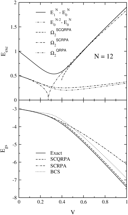
Figure 1: Ground-state energy $E_{gs}$ and excitation energy of the first $0^{+}$ state $E_{exc}$ as a function of the variable $V=g\Omega/2\epsilon$ described in the text and for particle number $N=12$ (energies are divided by $2\epsilon$). The spin of the levels is $J=11/2$. The results refer to exact calculations (solid line and double-dot dashed line), BCS (dotted line), RPA and QRPA (dot-dashed line), SCQRPA (dashed line) and SCRPA (double-dash dotted line). (Note that SCRPA and SCQRPA solutions co-exist over a wide range of $V$-values).

Let us first discuss the case with $N=12$, i.e. the lower level is filled in the absence of correlations. We call this the half-filled or symmetric case. In Fig.1 we show in the upper panel the excitation energies. Let us consider the well known scenario of the standard RPA. Before the phase transition to the superfluid phase we work with the unconstrained Hamiltonian. One obtains two eigenvalues with the interpretation of differences of ground-state energies, differing by two units in mass $2\mu^{\pm}=\pm(E^{N\pm 2}_{0}-E^{N}_{0})$. They are evidently related to the chemical potential and in standard particle-particle RPA (pp-RPA) they are given by

$$\Omega_{a}&=2\mu^{+}=-g+\sqrt{g+\epsilon}\sqrt{\epsilon+g(1-2\Omega)},\\ \Omega_{r}=-2\mu^{-}=g+\sqrt{g+\epsilon}\sqrt{\epsilon+g(1-2\Omega)},$$ (128)

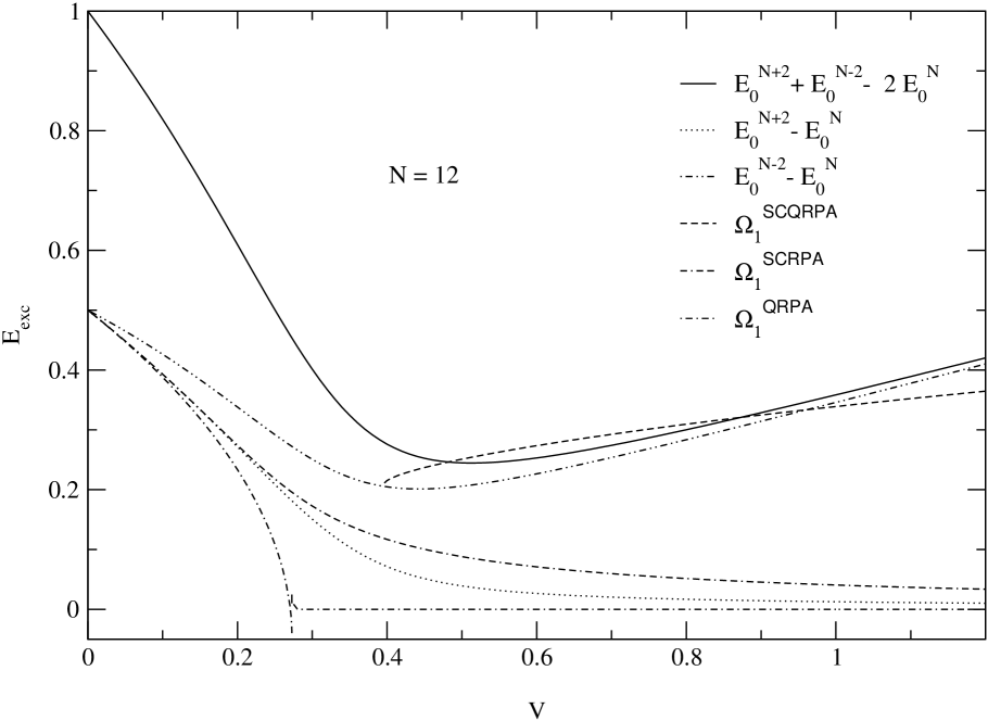
Figure 8: Excitation energy of the soft (spurious) mode (energies are divided by $2\epsilon$) as a function of the variable $V=g\Omega/2\epsilon$ described in the text and for particle number $N=12$. The spin of the levels is $J=11/2$. The results refer to exact calculations (solid line, dotted line and double-dot dashed line), RPA and QRPA (dot-dashed line), SCQRPA (dashed line) and SCRPA (double-dash dotted line).

where $\Omega_{a}$ and $\Omega_{r}$ correspond to the addition and removal phonons of the pp-RPA, respectively. In Fig.1 the case $-2\mu^{-}$ is shown and we will discuss the case $2\mu^{+}$ separately below in Fig.8. We see on the graph the usual result, namely that $-2\mu^{-}$ drops to zero at the phase transition point (strictly speaking only in the large $\Omega$ limit). After the phase transition point we work with the constrained Hamiltonian (19) in the BCS quasi-particle representation. The QRPA eigenvalue (127) is also shown in Fig.1. The Goldstone mode (127) at zero energy corresponds to a rotation in gauge space whereas the second eigenvalue corresponds to the ”$\beta-$vibration” of the nucleus with $N$ particles b18 . This difference in interpretation is also well born out in the SCQRPA in comparison with the exact solution. We see that in the transition region SCRPA shows a tremendous improvement over RPA and that SCRPA follows the exact value of $-2\mu^{-}$ even far beyond the phase transition point (as defined by BCS theory) where no RPA solution exists. It is also to be noticed that the sharp phase transition seen in RPA-QRPA is an artifact of the theory and that in reality the phase transition is completely washed out due to the finiteness of the system. The fact that the ”spherical” SCRPA solution co-exists with the ”deformed” SCQRPA solution over a wide parameter range representing different energy states of the system is a quite unique situation. In all other model cases where we have investigated the ”spherical-deformed” transition the ”spherical” solution ceased to converge numerically b25 beyond a certain critical coupling. This, however, is no proof that the ”spherical” solution does not also exist far in the deformed region representing physical states. It may be that in those works simply the method for the numerical solution was not sophisticated enough. This is a point to be investigated in the future. In the superfluid (deformed) region SCQRPA still is superior to QRPA but the improvement is less spectacular. This stems from the fact that the transformation to BCS quasi-particles effectively accounts already for some supplementary correlations in QRPA and thus the differences with exact and SCQRPA solutions become less important than in the non superfluid regime. A feature which is to be remarked in Fig.1 is the fact that SCRPA and SCQRPA do not smoothly match in the transition region whereas RPA and QRPA have a certain continuity at the transition point. However, we see that SCRPA and SCQRPA describe two physically very distinct states which do not have any contact in the exact case neither and therefore it is not astonishing that SCRPA and SCQRPA do not join. This mismatch has as a consequence that there also exists a rupture in the ground-state energy as a function of interaction as is seen in the lower panel of Fig.1. Again SCQRPA results improve strongly over BCS ground-state energies in the deformed region.

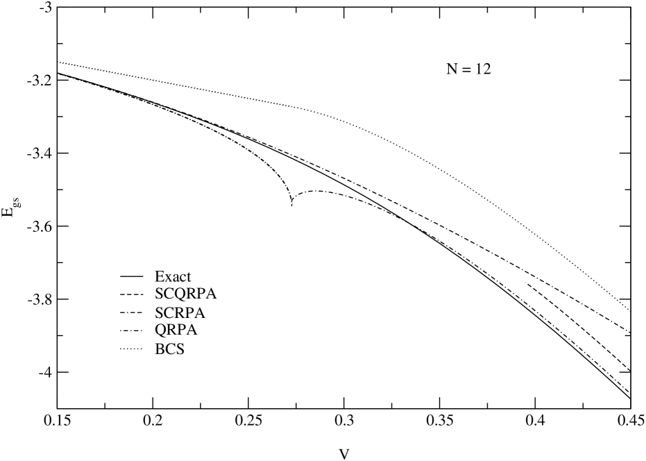
Figure 2: Zoom on the ground-state energy $E_{gs}$ as a function of the variable $V=g\Omega/2\epsilon$ described in the text and for particle number $N=12$ (energies are divided by $2\epsilon$). The spin of the levels is $J=11/2$. The results refer to exact calculations (solid line), BCS (dotted line), RPA and QRPA (dot-dashed line), SCQRPA (dashed line) and SCRPA (double-dash dotted line).

So far we have omitted the discussion of two items of the case considered in Fig.1 which are slightly subtle. The first is the fact that the QRPA shows two eigenvalues : the ”$\beta-$vibration” and the Goldstone mode at zero energy (”the pair rotation mode”), whereas we have not shown the corresponding low energy mode of SCQRPA. We will below devote an extra paragraph to this issue. The second point is that we have not shown in Fig.1 the QRPA values for the ground-state energies. We show this separately in an enlarged scale around the transition point in Fig.2. We there see that QRPA overbinds in the transition region but that further to the right of the transition region QRPA values are closer to the exact solution than the ones from SCQRPA. This is a paradoxical result which systematically repeats itself for all other configurations we will consider below. However, the seemingly ”better agreement” is an artifact of the QRPA which has already been encountered in others cases b25 . We want to argue as follows : SCQRPA is in itself a well defined theory, resulting from the variational principle (57) for two body correlation functions. One also can consider it as a HFB approach for Fermion pairs. The Pauli principle is respected in an optimal way, since at no point a bosonization of Fermion pair operators is introduced and the Pauli principle is only violated in the truncation of (115) which is a very fast converging series. However, any approximation to the full SCQRPA scheme necessarily diminishes the respect of the Pauli principle what simulates more correlations than there should be. Since for the present model case the SCQRPA ground-state energy is systematically above the exact one (under binding), it may happen that, when the Pauli principle constraint is released in going from SCQRPA to QRPA, the corresponding gain in energy is such that, accidentally, the QRPA ground-state energy practically coincides with the exact values over a wide rang of parameters. We think that this is what happens in this model not only for the configuration in Fig.1 but systematically for all types of degeneracies and all fillings. We will not discuss this issue for the other cases any more in this work. We again should mention that we have found such fortuitous coincidences already in other works b25 . However, in more realistic cases ones usually finds that the standard RPA strongly overbinds with respect to the exact values b26 .

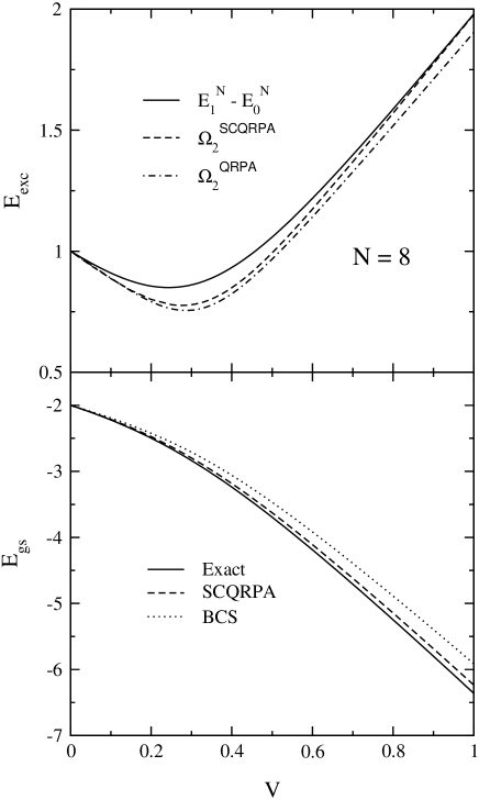
Figure 3: As in Fig.1 but for $N=8$.

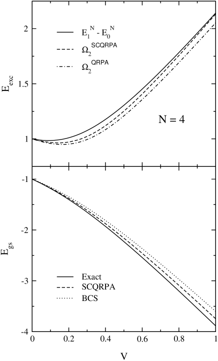
Figure 4: As in Fig.1 but for $N=4$.

Let us now discuss situations where either the lower or upper levels are only partially filled. Like in the one level pairing case these configurations always show a non trivial BCS solution, i.e. they are always in the superfluid regime independent of $V$. Let us look at Fig.3 with $J=11/2$ and $N=8$ that is the lower level partially filled for $V=0$. In the upper panel the high lying eigenvalue of the SCQRPA equations is shown against the exact value. We see that there is some improvement of SCQRPA with respect to QRPA but it is not spectacular. It is similar to the case of Fig.1 where in the superfluid region the improvement, for reasons already explained above, is modest. For the ground-state energy there is quite strong improvement over BCS theory. The QRPA result is not shown but the situation is the same as already explained above. The cases $J=11/2$, $N=4$ and $N=14$ shown in Fig.4-5 are qualitatively similar.

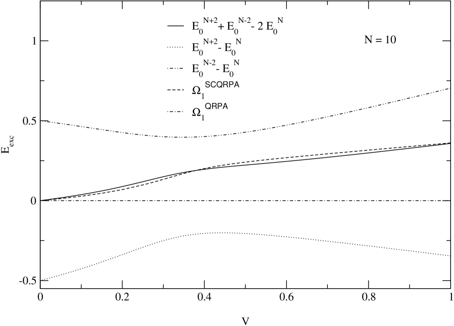
Figure 6: Excitation energy of the soft (spurious) mode (energies are divided by $2\epsilon$) as a function of the variable $V=g\Omega/2\epsilon$ described in the text and for particle number $N=10$. The spin of the levels is $J=11/2$. The results refer to exact calculations (solid line, dotted line and double-dot dashed line), QRPA (dot-dashed line), and SCQRPA (dashed line).

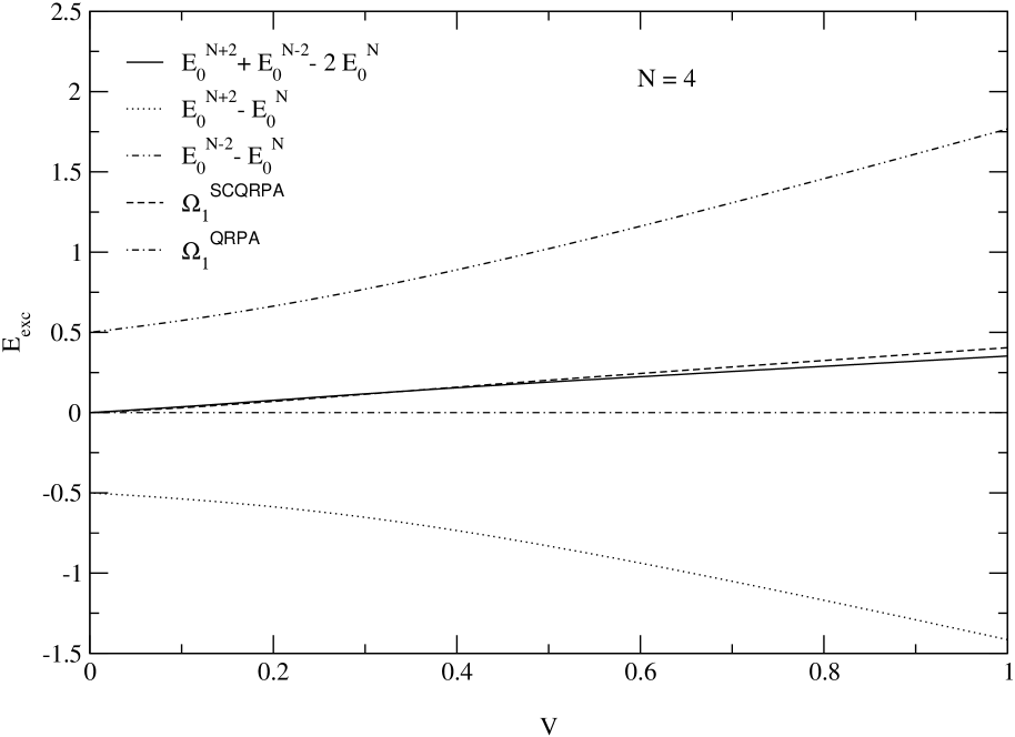
Figure 7: As in Fig.6 but for $N=4$.

Let us now come to the low lying eigenvalue of SCQRPA which in QRPA corresponds to the zero energy eigenvalue (Goldstone or spurious mode). In Fig.6 we show the low lying eigenvalue for the case $J=11/2$ and $N=10$. We see that this eigenvalue follows very precisely the difference $2(\mu^{+}-\mu^{-})=E^{N+2}_{0}+E^{N-2}_{0}-2E^{N}_{0}$ of the two chemical potentials $2\mu^{+}=E^{N+2}_{0}-E^{N}_{0}$ and $2\mu^{-}=E^{N}_{0}-E^{N-2}_{0}$ as obtained from the exact calculation. This identification makes indeed sense : since we are in the symmetry broken phase the SCQRPA system can not distinguish between $N\pm 2$ states. For large $N$ both $2\mu^{+}$ and $2\mu^{-}$ tend individually to Goldstone modes but for finite $N$ it definitely is reasonable to define the difference between $2\mu^{+}$ and $2\mu^{-}$ as the low lying excitation and it is this combination which shows up as low lying mode in the SCQRPA calculation. This is confirmed in looking at other configurations : in Fig.7 we show the case $J=11/2$, $N=4$ and in fact we find analogous scenarios for all configurations we investigated, besides one : this is the symmetric case with $J=11/2$, $N=12$. In the Fig.8 we see that the picture is slightly different from the rest of the cases. This stems from the fact that in the symmetric case we have a transition from the superfluid to the non superfluid regime which is absent in the other partially filled cases. We also see that the values for $2\mu^{+}$ and $2\mu^{-}$ are very asymmetric, $2\mu^{+}$ apparently taking the role of the Goldstone mode alone. Also the agreement of the low lying SCQRPA solution $\Omega_{1}$ is slightly less good than in all other cases.

Let us also add some remarks why in SCQRPA there is, contrary to QRPA, no exact Goldstone mode at zero energy. This is relatively easy to understand : in quasi-particle representation the number operator is given by (48), (49). One can check that in QRPA the terms $\alpha^{\dagger}\alpha$, if they were included, completely decouple of the QRPA equations. Therefore, in QRPA it is as if one had used the full particle number operator and therefore a particular solution of the QRPA equations is $Q^{\dagger}\equiv\hat{N}$ and with $[H,\hat{N}]=0$ we get the zero eigenvalue in the Equation of Motion (EOM) approach. This argumentation is no longer true in SCQRPA where the terms $\hat{N}_{q,j}$ (49) of the number operator contribute in principle to SCQRPA. However, we can not include them in the RPA operator because these are hermitian pieces leading to non-normalizable eigenstates. Therefore $Q^{\dagger}=\hat{N}$ as a particular solution only holds in QRPA but not in other cases such as SCQRPA. However as a benefit, we see in the preceding figures that we can identify the finite value of $\Omega_{1}$ with a particular rotational frequency in gauge space of the exact solution of the problem. On the other hand in realistic situation one can include in the RPA operator terms of the form $\alpha^{\dagger}_{k}\alpha_{k^{\prime}}$ for $k\neq k^{\prime}$ b12 . Only the hermitian operators $\alpha^{\dagger}_{k}\alpha_{k}$ have to be excluded for the reason already mentioned. These components correspond in an infinite system to momentum transfer zero and they are thus of zero measure. Therefore in an infinite system we have again full restoration of symmetry.

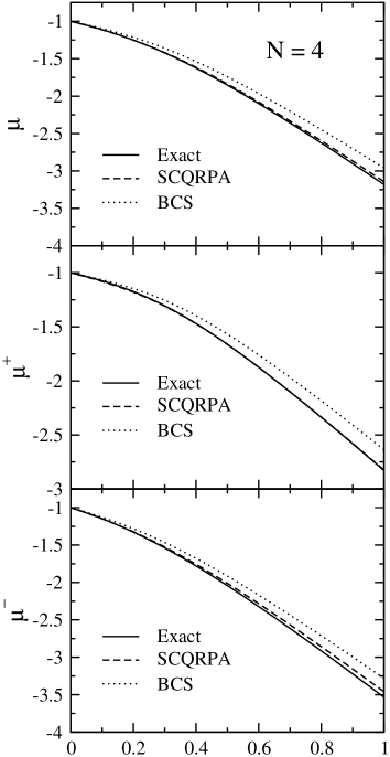
Figure 9: Comparison between SCQRPA, BCS and exact results for the chemical potentials $\mu=\frac{1}{2}(\mu^{+}+\mu{-})$ and $\mu^{\pm}=\pm\frac{1}{2}(E^{N\pm 2}_{0}-E^{N}_{0})$, for particle number $N=4$. The spin of the levels is $J=11/2$. The results refer to exact calculations (solid line), SCQRPA (dashed line) and BCS (dotted line).

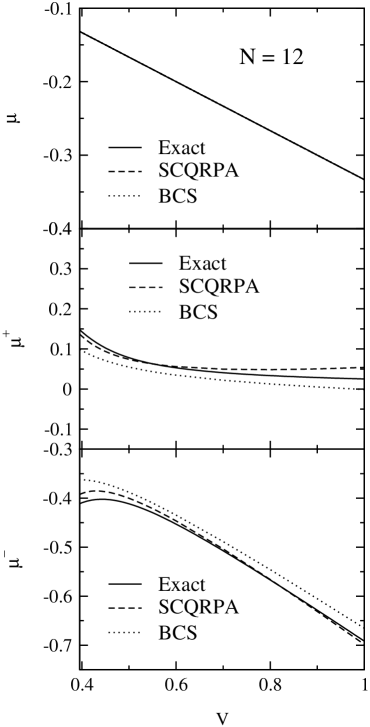
Figure 11: As in Fig.9 but for $N=12$.

Other quantities which are interesting to be calculated within the SCQRPA formalism are the chemical potentials directly from differences of ground-state energies. For example in Fig.9-10 we show $\mu^{\pm}=\pm\frac{1}{2}(E^{N\pm 2}_{0}-E^{N}_{0})$ where the individual ground-state energies are obtained directly from separate SCQRPA calculations. We see for $J=11/2$ and $N=4\;\text{and}\;8$ that the agreement between SCQRPA results and exact values is excellent and in any case a strong improvement over BCS theory can be noticed. The same is true for the chemical potential $\mu$ as obtained from $\mu=\frac{1}{2}(\mu^{+}+\mu^{-})$ in the exact calculation. This latter which is an average chemical potential should be identified with the Lagrange multiplier $\mu$ used for restoring the symmetry of the good particle number (10) in BCS and SCQRPA. This identification is shown in each upper panel in Fig.9-11. In Fig.11 we show the results for $\mu$ and $\mu^{\pm}$ for the symmetric case $J=11/2$ and $N=12$. We see that again the same remarks as for the asymmetric cases hold true. However, we notice the particular situation that for $\mu$ the exact, BCS, and SCQRPA solutions coincide exactly. This has to do with the specific symmetries in the half-filled case.

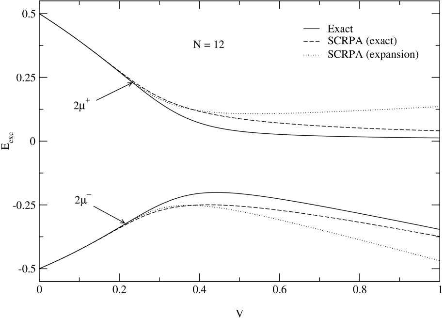
Figure 12: Excitation energies $2\mu^{+}$ (upper lines) and $2\mu^{-}$ (energies are divided by $2\epsilon$) as a function of the variable $V=g\Omega/2\epsilon$ described in the text and for $N=12$. The spin of the levels is $J=11/2$. The full lines correspond to the exact results, the broken lines to SCRPA with occupation numbers calculated with the wave function (129), and dotted lines to SCRPA with occupation numbers from the expansion (115).

It is also interesting to show the chemical potentials $2\mu^{+}$ and $2\mu^{-}$ in a symmetric way as done in b27 . This also gives us the occasion to study the accuracy of our approximation (115) and (118) for the occupation numbers. Lets us first of all say that we have here a quite unusual situation for SCRPA : the solution in the spherical, i.e. non superfluid basis, exists far into the superfluid regime. Usually in other models the solution of SCRPA in the spherical basis can be found up to interaction values slightly beyond the mean field transition point but here very reasonable values for the chemical potentials $2\mu^{\pm}$ are obtained for all values of $V$ as seen in Fig.12. This was also found in the work by Passos and al. b27 . It should be mentioned, however, that maintaining the spherical basis gives much less good results for the ground-state energy as seen in Fig.1. Indeed after the transition point the ground-state energy values deviate quite strongly from the exact results. In Fig.12 we calculate the expectation values $\langle\hat{N}_{i}\rangle$ and $\langle\hat{N}_{i}\hat{N}_{j}\rangle$ with the exact RPA ground-state b13

$$|RPA\rangle=\sum_{l=0}^{\Omega}\big{(}\frac{Y}{X}\big{)}^{l}\big{(}A^{\dagger}_{1}\big{)}^{l}\big{(}A^{\dagger}_{-1}\big{)}^{\Omega-l}|-\rangle,$$ (129)

where $X$, $Y$ are the RPA amplitudes, defined with the addition (P) and removal (R) phonons of the particle-particle RPA and satisfying the normalization condition $X^{2}-Y^{2}=1$. This gives the broken lines. If we calculate the same values from our limited expansion (115) then the dotted lines are obtained. We see that beyond the transition point the solution becomes extremely sensitive to approximations. Indeed our approximated values deviate quite a bit from the ones calculated with the full wave function $|RPA\rangle$.

A quantity which is particularly sensitive to the correct treatment of correlations are the occupation numbers. For example, for the particle number in the upper level we obtain

$$\langle\hat{N}_{1}\rangle=(u_{1}^{2}-v_{1}^{2})\langle\hat{N}_{q,1}\rangle+2\Omega v_{1}^{2}$$ (130)

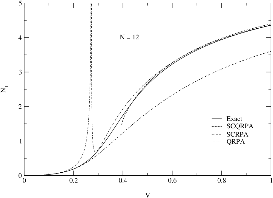
Figure 13: Particle number in the upper level $N_{1}$ as function of the variable $V=g\Omega/2\epsilon$ described in the text and for $N=12$. The spin of the levels is $J=11/2$.The results refer to exact calculations (solid line), SCQRPA (dashed line), SCRPA (double-dash dotted line) and QRPA (dot-dashed line).

and the result is shown in Fig.13 for the superfluid and non superfluid regimes. Once again we see that the change around the phase transition is not continuous. Still with SCQRPA one notices a tremendous improvement over standard QRPA for which the amplitudes diverge at the critical point. Indeed it is just in such quantities as occupation numbers where the full superiority of SCQRPA over its linearized version of QRPA is fully born out. Before finishing this section, we will explain how we proceeded to make the QRPA and RPA calculation of $\langle\hat{N}_{q,1}\rangle$ in both regions normal and superfluid. We use the first order of the bosonic expansion of the $\hat{N}_{q,1}$, i.e. the first order of the expansion shown in (115), where it is sufficient to put $P^{\dagger}_{1}=B^{\dagger}_{1}$. Thus, with the commutation rules (18), we find

$$\langle\hat{N}_{q,1}\rangle=\frac{2(Y^{2}_{1,1}+Y^{2}_{1,2})}{(1+\frac{2}{\Omega}(Y^{2}_{1,1}+Y^{2}_{1,2}))}.$$ (131)

In linearizing this expression, we obtain

$$\langle\hat{N}_{q,1}\rangle=2(Y^{2}_{1,1}+Y^{2}_{1,2}).$$ (132)

It is interesting to detail this calculation, since it is useful to see analytically the QRPA and RPA results for the particle number in the upper level close the transition point. It is well known that the two excitation modes in the RPA method converge to zero at the transition point, then the corresponding RPA amplitudes tend to infinity, what explains the divergence of $\langle\hat{N}_{1}\rangle$. In the superfluid zone, we mention that we neglected the RPA amplitudes corresponding to the Goldstone (spurious) mode when we make the calculation of $\langle\hat{N}_{1}\rangle$.

A constant concern for superfluidity or superconductivity in finite systems is that the quasi-particle transformation (11) does not preserve good particle number. Even though one fixes particle number in the mean with the help of a Lagrange multiplier, the contamination of expectation values with components which have wrong particle number can be quite important. This is for instance the case for atomic nuclei. That is why, very early, one has thought of how to improve BCS theory with respect to particle number conservation. One quite popular approach is to project the BCS wave function on good particle number. An approximation to this relatively heavy scheme is the approximate particle number projection by Lipkin-Nogami b28 . It is therefore interesting to investigate how much SCQRPA improves on the spread in particle number. We therefore will calculate

$$(\Delta N)^{2}=\langle\hat{N}^{2}\rangle-{\langle\hat{N}\rangle}^{2}$$ (133)

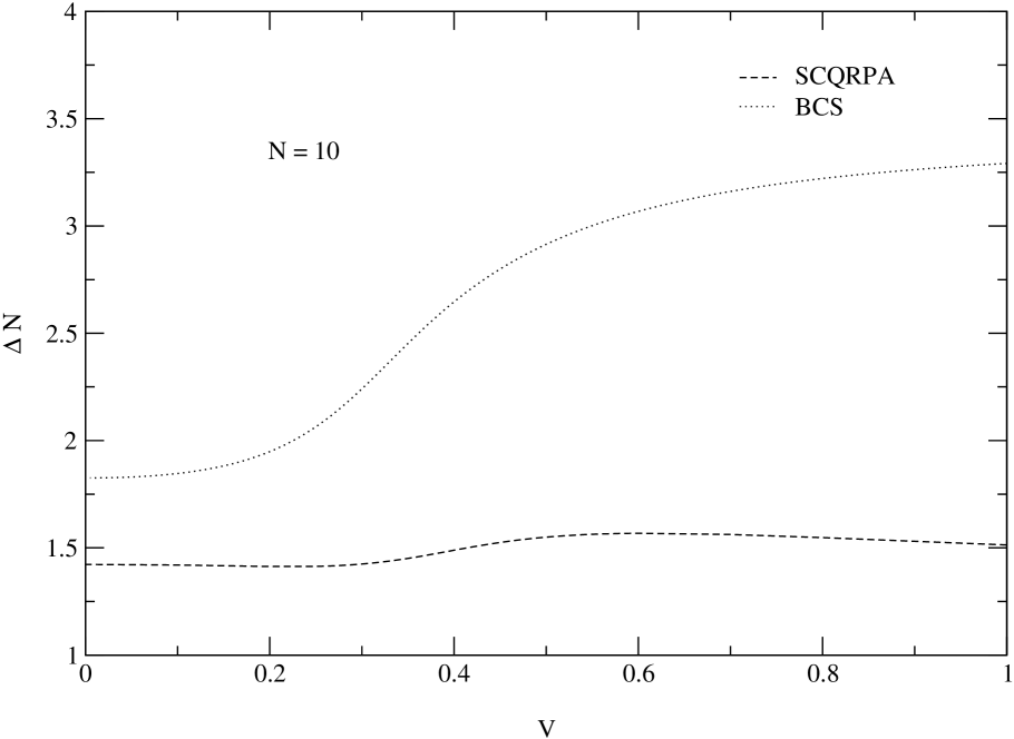
Figure 14: Variance as a function of the variable $V=g\Omega/2\epsilon$ described in the text and for particle number $N=10$. The spin of the levels is $J=11/2$. The results refer to SCQRPA calculations (dashed line) and BCS (dotted line).

with $\hat{N}=\hat{N}_{1}+\hat{N}_{-1}$ the particle number operator and $\hat{N}_{j}$ given by (49) within SCQRPA. The terms involving bilinear forms in $P^{\dagger}_{j}$, $P_{j}$ are as usual directly expressed by the RPA amplitudes and for the quasi-particle occupation number operators we use (115)-(118). Then $\Delta N$ can be calculated and the results for various configurations are shown in Fig.14-16. We see that the spread in particle number is strongly reduced over BCS values reaching typical factors two to three. We, however, see that $\Delta N$ even in SCQRPA acquires non vanishing sizable values. This is an expression that particle number is not completely restored. We will see in section VI how one eventually can improve on this. We also tried to evaluate $\Delta N$ in standard QRPA in applying a lowest order bosonization of the expression. However, due to the non-normalizable Goldstone mode we ran into troubles with this procedure and could not reach a definite conclusion on this point.

Another interesting aspect which can be studied with our model is the question whether the pairing correlations, with respect to BCS, have been enhanced or weakened due to the SCQRPA correlations. To this end we define the following quantal expression for the correlation function

$${\cal C}=\frac{1}{\Omega}\sum_{j=\pm 1}\bigg{(}\langle A^{\dagger}_{j}A_{j}\rangle-\frac{1}{4\Omega^{2}}\langle\hat{N}_{j}\rangle\langle\hat{N}_{j}\rangle\bigg{)}.$$ (134)

This expression reduces to the following expression when evaluated with the BCS ground-state

$${\cal C}_{BCS}=\sum_{j=\pm 1}u^{2}_{j}v^{2}_{j}.$$ (135)

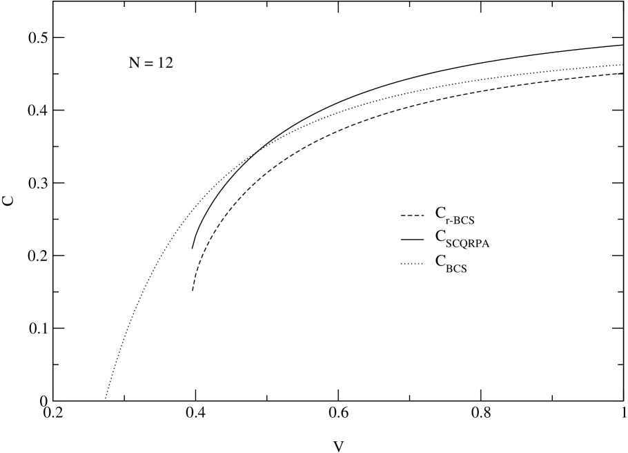
Figure 17: Correlation function ${\cal C}$ as a function of the variable $V=g\Omega/2\epsilon$ described in the text and for particle number $N=12$. The spin of the levels is $J=11/2$.The results refer to SCQRPA (solid line), renormalized BCS (dashed line) and standard BCS (dotted line).

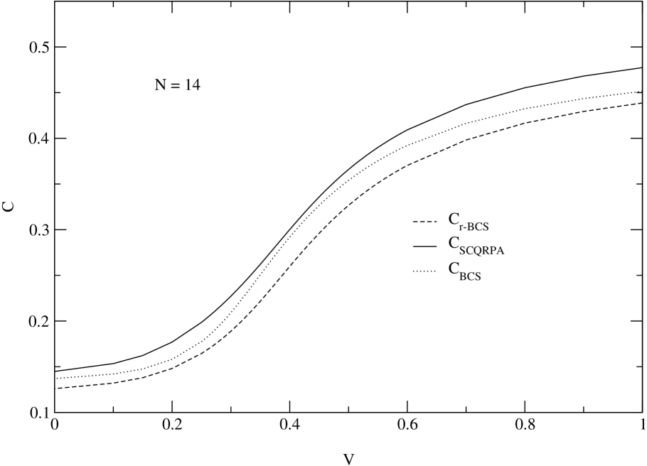
Figure 18: As in Fig.17 but $N=14$.

Multiplying (135) with $g^{2}\Omega^{2}$ yields the standard BCS gap squared. We, however, refrain from multiplying (134) or (135) with $g^{2}\Omega^{2}$, since the renormalized gap from (96) is level dependent. Often also (134) is given in a non diagonal form b34 but having difficulties to express non diagonal densities with SCQRPA amplitudes we will not consider the non diagonal form here. We therefore evaluate (134) in three approximations : we can express (134) in terms of $P^{\dagger}_{j}$, $P_{j}$ and $\hat{N}_{q,j}$ operators and then take the expectation value with the SCQRPA ground-state. The equations (56), (115) and (117) then allow to express ${\cal C}$ in terms of the SCQRPA amplitudes $X_{j,\nu}$, $Y_{j,\nu}$. We will call this ${\cal C}_{SCQRPA}$. We also evaluate (135) in the standard BCS approximation which is (134). However, we also calculate (135) with $u_{j}$, $v_{j}$ amplitudes from the renormalized BCS (r-BCS) theory, i.e. from (95) with $\Delta_{i}$ solution of (96). The results are shown in Fig.17 and Fig.18 for $N=12$ and $N=14$ respectively (the case $N=10$ gives exactly same results as $N=14$). We see that r-BCS gives with respects to BCS less correlations. Eventually this suppression of pairing can be put into analogy with gap suppression in infinite neutron matter from renormalized theories b3 (see discussion in the introduction). However, the suppression of pairing correlation in r-BCS is misleading in our model, since, on the contrary, the full SCQRPA gives mostly an enhancement of pair correlations with respect to BCS. It is not obvious whether this conclusion can be taken over to the infinite matter case. It may, however, be indicated that the renormalized gap equations from screening (RPA) type correlations should be carefully treated consistently with the evaluation of two body correlation function before definite conclusions can be reached.

Table 1: Results for the ground-state energy (in arbitrary units) vs the variable $V=g\Omega/2\epsilon$ described in the text. The spin of the levels is $J=19/2$ and the number of particles is $N=20$.

V	Exact	SCQRPA	BF-RPA	QRPA	BCS
-0.50	-18.55446	-18.55410	-18.55360	-18.56890	-18.00000
-0.45	-18.66849	-18.66821	-18.66784	-18.67924	-18.20000
-0.40	-18.78706	-18.78686	-18.78660	-18.79474	-18.40000
-0.35	-18.91072	-18.91058	-18.91040	-18.91592	-18.60000
-0.30	-19.04010	-19.04001	-19.03990	-19.04338	-18.80000
-0.25	-19.17600	-19.17594	-19.17588	-19.17787	-19.00000
-0.20	-19.31939	-19.31936	-19.31933	-19.32031	-19.20000
-0.15	-19.47153	-19.47151	-19.47150	-19.47188	-19.40000
-0.10	-19.63406	-19.63405	-19.63405	-19.63415	-19.60000
-0.05	-19.80919	-19.80919	-19.80919	-19.80919	-19.80000
0.00	-20.00000	-20.00000	-20.00000	-20.00000	-20.00000
0.05	-20.21101	-20.21101	-20.21101	-20.21102	-20.20000
0.10	-20.44921	-20.44918	-20.44917	-20.44953	-20.40000
0.15	-20.72625	-20.72599	-20.72593	-20.72899	-20.60000
0.20	-21.06339	-21.06130	-21.06100	-21.08080	-20.80000
0.25	-21.50260	-21.48733	-21.48640	-21.64174	-21.00000
0.30	-22.12491	-22.03638	-22.03620	-22.13484	-21.37193
0.35	-23.03321	-22.80453	-22.77899	-22.99299	-22.21880
0.40	-24.24609	-23.99588	-23.97001	-24.21285	-23.37895
0.45	-25.68929	-25.42829	-25.39821	-25.65779	-24.74795
0.50	-27.29077	-27.01885	-26.98390	-27.25633	-26.26316

V Comparison with other recent works

The two level pairing model has recently served as a testing ground for various generalizations of BCS theory. In spirit the work which comes closest to the present is the one of Sambataro and Dinh Dang b23 . Instead of treating quasi-particle pair operators directly as we do here, they bosonize them (with a method developed in b23 ) and expand the Hamiltonian (1) in terms of these Bosons up to fourth order. A Bogoliubov transformation of the Boson operators quite analogous to our Bogoliubov transformation of Fermion pair operators (11) is then performed and the corresponding non linear Hartree-Fock-Bogoliubov equation are written down. Again they are quite analogous to our SCQRPA equations. The coefficients of quasi-particle transformation are obtained, as usual, in minimizing the ground-state energy (see also our procedure (88)) with respect to the transformation coefficients. As in our case equations are obtained which couple back to the bosonic HFB, i.e. the RPA amplitudes. The coupled system of equations for fermionic and bosonic transformation amplitudes is then solved self-consistently. For better comparison we actually, on purpose, have chosen most of the configurations in $J$ and $N$ the same as in b23 . Since in b23 $J=11/2$, what is a rather high degeneracy of the levels, the Fermion pair operators are quite collective and a bosonization certainly is a valid procedure. Not unexpectedly, therefore, the results of the present work are very close to the ones presented in b23 . A detailed comparison shows that our results are systematically closer to the exact ones by a very small amount. This may be due to the fact that we never bosonize and treat the Fermion pair commutation rules exactly but the difference is too small for drawing any definite conclusion. In b23 , Sambataro and al. show an explicit comparison of results referring to the symmetric case with $J=19/2$. We also can make such a comparison for the ground-state energy referring to the same configuration. It is given in TABLE.1, where we show the results for four different many-body approaches : our approach (SCQRPA), approach of Sambataro and al. (BF-RPA) b23 , standard Quasi-Particle RPA (QRPA) b24 and the BCS method b18 . Of course, we recall that in our approach, we use the Self-Consistent particle-particle RPA in the normal fluid zone, while, in the superfluid region we use the generalized version of SCRPA that is SCQRPA. In order to accentuate the differences one would have to go to configurations with much lower degeneracies where the constraints from the Pauli principle become much more severe. For example the SCRPA approach has been applied to the case $J=1/2$ with $N=2$ in b7 and the exact result was recovered. It would be interesting to see how the approach with the bosonization b23 performs in that case. In spite of being very similar in general spirit to the work in b23 we have solved and considered several additional problems which remained open in b23 . In first place this concerns the low lying eigenvalue of SCQRPA. No interpretation of this important root was given in b23 . We, however, suppose that the results in b23 for this state (no numerical values have been given) can be equally interpreted as the difference $2(\mu^{+}-\mu^{-})$ as in our case. Another quantity which was not considered in b23 is the number fluctuation. Again we believe that corresponding values would be close to the ones found here. Also the transition to the non superfluid regime has not been treated in b23 . However, probably all these aspects will be quite similar in both approaches as long as a bosonization of the Fermion pair operators is valid. We think, however, that it does not cost much to avoid bosonization altogether as with the SCQRPA approach.

Also in the work by Passos and al. b27 the SCRPA method was applied to the present model. However, only the non superfluid formulation, i.e. SCRPA, was studied. The results are quite analogous to ours. In addition in b27 a further approximation, half way between RPA and SCRPA, the so-called renormalized RPA (r-RPA) where only the single-particle occupation numbers are allowed to be affected by ground-state correlation, has been considered. The astonishing finding there was that the exact occupation numbers are almost perfectly reproduced over the whole range of the coupling constant with r-RPA but not with SCRPA which under shoots the correlations. This was interpreted in b27 as a positive feature of r-RPA over SCRPA. We can not follow this conclusion from our experience with SCRPA in this and other works b7 . As we outlined above, any relax of the severe constraints of the Pauli principle respected in SCRPA will inevitably lead to more correlations as there should be. It can happen by accident that if one relaxes the Pauli principle just by the right amount that one falls more or less on the exact values. This is what happened for the QRPA ground-state energy discussed above and apparently it is also what happens for the occupation numbers in r-RPA. However, we think this result can not be generalized and for other models or physical situations the scenario may be completely different. The only really trust worthy theory is the full SCRPA approach, since it can be derived from a variational principle. If the results are not good, one must improve on SCRPA (i.e. include e.g. higher configurations) and not approximate it.

In the work by Hagino and Bertsch b24 the QRPA approach is advocated. This in the spirit to have a numerically viable alternative to projected BCS and the method by Nogami-Lipkin b28 . It is certainly true that in realistic cases SCRPA is numerically very demanding, though probably not impossible to solve with modern computers. Then, of course, in a first step it is worthwhile to investigate standard QRPA. This is for instance true if one intends to do large scale calculations for a great number of nuclei b24 . However, one should always remember that standard QRPA may have quite important failures which certainly will be most prominent in situations where the system is close to a phase transition.

VI The question of a second constraint on the particle number variance

As we have seen above, with respect to BCS the SCQRPA reduces the spread in particle number by an important factor. However, the variance $\Delta N$ is still appreciable and one can ask the question whether it is not possible to further improve the theory on this point. A natural idea which comes to mind is that instead of fixing only $\langle\hat{N}\rangle=N$, one could at the same time fix $\langle\hat{N}\hat{N}\rangle=N^{2}$ with a second Lagrange multiplier. Since in SCQRPA the number of variational parameters is largely increased with respect to BCS one could imagine that there is indeed enough freedom for constraining the particle number fluctuation to zero. The Hamiltonian to be considered is therefore

$$H^{\prime}=H-\mu_{1}\hat{N}-\mu_{2}{\hat{N}}^{2}.$$ (136)

Let us immediately give our conclusion : in the two level pairing case we could not find a solution to this problem. The system of non linear equations with the two constraints $\mu_{1}$ and $\mu_{2}$ is quite complex and in spite of considerable numerical effort we did not have success to get the solution converged. We were not able to decide whether the difficulty is purely numerical or whether there is a principal problem. In fact we were at first encouraged by results we obtained in the one level pairing case (the seniority model). The outcome of employing the second constraint was that the one level model was solved exactly. In spite of being a somewhat trivial model which certainly limits the conclusions, it may be interesting to show how this goes. The Hamiltonian to be considered is now

$$H^{\prime}=H-\mu_{1}\hat{N}-\mu_{2}{\hat{N}}^{2}.$$ (137)

where $\mu_{1}$ and $\mu_{2}$ are two Lagrange multipliers fixing $\langle\hat{N}\rangle=N$ and $\langle\hat{N}^{2}\rangle=N^{2}$ and

$$H=-g\Omega A^{\dagger}A$$ (138)

with in analogy to (2) $A^{\dagger}=\frac{1}{\sqrt{\Omega}}\sum_{m>0}a^{\dagger}_{m}a^{\dagger}_{-m}$, and where we put the origin of energy at the single-particle level. As in the two level case we transform to quasi-particles and with only one level the SCQRPA equation reduce to a $(2\times 2)$ eigenvalue problem

$$\pmatrix{A&B\cr-B&-A\cr}\pmatrix{X\cr Y\cr}=E\pmatrix{X\cr Y\cr};\quad X^{2}-Y^{2}=1$$ (139)

where in analogy with (74)

$$A = 2(g-4\mu_{2})\bigg{\{}(2v^{2}(1-v^{2})-1)XY-v^{2}(1-v^{2})(1+2Y^{2}-\Omega\frac{1-2\frac{\langle\hat{N}_{q}\rangle}{\Omega}+\frac{\langle\hat{N}_{q}^{2}\rangle}{\Omega^{2}}}{1-\frac{\langle\hat{N}_{q}\rangle}{\Omega}})\bigg{\}},$$ (140)

$$B = 2(g-4\mu_{2})\bigg{\{}(6v^{2}(v^{2}-1)+1)XY-v^{2}(1-v^{2})(1+2Y^{2}-\Omega\frac{1-2\frac{\langle\hat{N}_{q}\rangle}{\Omega}+\frac{\langle\hat{N}_{q}^{2}\rangle}{\Omega^{2}}}{1-\frac{\langle\hat{N}_{q}\rangle}{\Omega}})\bigg{\}}.$$ (141)

The Bogoliubov transformation to quasi-particles is obtained as for the case of two levels

$$\pmatrix{h&\Delta\cr\Delta&-h\cr}\pmatrix{u\cr v\cr}=\tilde{\epsilon}\pmatrix{u\cr v\cr}$$ (142)

with in close analogy to the expression (88) of the two levels

$$h&=-(g+4\mu_{2}\Omega)v^{2}-\mu_{1},\\ \Delta=(g\Omega+4\mu_{2})uv-(g-4\mu_{2})uv\bigg{\{}2(XY+Y^{2})+\frac{\langle\hat{N}_{q}\rangle-\frac{\langle\hat{N}_{q}^{2}\rangle}{\Omega}}{1-\frac{\langle\hat{N}_{q}\rangle}{\Omega}}\bigg{\}},\\ \tilde{\epsilon}=\sqrt{h^{2}+\Delta^{2}}.$$ (143)

In addition to the SCQRPA equations (139) we have two further equations which, in principle, allow us to find the Lagrange multipliers $\mu_{1}$ and $\mu_{2}$ (see, however, below)

$$N&=\langle\hat{N}\rangle=(u^{2}-v^{2})\langle\hat{N}_{q}\rangle+2\Omega v^{2},\\ N^{2}=\langle\hat{N}^{2}\rangle=(u^{2}-v^{2})^{2}\langle\hat{N}_{q}^{2}\rangle+8\Omega u^{2}v^{2}(1-\frac{\langle\hat{N}_{q}\rangle}{\Omega})(XY+Y^{2})+4\Omega v^{2}(u^{2}+\Omega v^{2})\cr+4v^{2}(\Omega(u^{2}-v^{2})-u^{2})\langle\hat{N}_{q}\rangle$$ (144)

We again see that eqs (144) reduce to the standard expressions, once, as in the HFB approximation, we pose $Y=\langle\hat{N}_{q}\rangle=\langle\hat{N}_{q}^{2}\rangle=0$. In the case of the seniority model the number equation (144) in the HFB approximation determines the amplitudes $u,v$ and then no freedom is left to impose $\Delta N=\sqrt{\langle\hat{N}^{2}\rangle-{\langle\hat{N}\rangle}^{2}}=0$. However, in the more general approach of SCQRPA there is more freedom and, as we will see, we will be able to satisfy the relation $\Delta N=0$ as well. For $\hat{N}_{q}$ and $\hat{N}^{2}_{q}$ we have the same relation as in (115) and (117). Again the system of equations is therefore closed.

Usually the number equation (144) and (144) are to be used for the determination of the chemical potential $\mu_{1}$ and the second Lagrange multiplier $\mu_{2}$ and the mean field equations for the amplitudes $u,v$ and $X,Y$. In the present case it is, however, more convenient to invert the role of mean field and number equations, since eqs (143) do not depend on the Lagrange multipliers and therefore readily allow to determine $v^{2}$ and $Y^{2}$ as a function of the particle number $N$. Inversely the two mean field eqs (139), (142) are linear in $\mu_{1}$ and $\mu_{2}$ and for instance it is seen that (139) directly yields

$$\mu_{2}=\frac{g}{4}$$ (145)

independent of the particle number $N$. Considering, the well known exact expression for the ground-state energy of the model b18

$$E_{0}=-\frac{g}{2}(\Omega+1)N+\frac{g}{4}N^{2}$$ (146)

we see from $\mu_{2}=\frac{\partial^{2}E_{0}}{\partial N^{2}}$ that (145) gives the exact value for the second Lagrange multiplier $\mu_{2}$. For the chemical potential $\mu_{1}$ we obtain from (142)

$$\mu_{1}=(g-4\mu_{2})\bigg{\{}(\Omega-1)v^{2}+(1-2v^{2})(XY+Y^{2}+\frac{1}{2}\frac{\langle\hat{N}_{q}\rangle-\frac{\langle\hat{N}_{q}^{2}\rangle}{\Omega}}{1-\frac{\langle\hat{N}_{q}\rangle}{\Omega}})\bigg{\}}-\frac{g}{2}\Omega-2\mu_{2}.$$ (147)

With relation (142) this gives $\mu_{1}=-\frac{g}{2}(\Omega+1)$ which again is the exact value. Furthermore, with (145) we have from (140), (141) that $A=B=0$ and therefore the RPA eigenvalue $E=0$. This means that, as in standard QRPA, SCQRPA yields a Goldstone mode at zero energy.This feature is very rewarding, since it signifies that the particle number symmetry is exactly restored.
It is well known that restoration of good particle number implies in this very simple model case that the model is solved exactly b18 . We have already seen that one obtains the exact values for $\mu_{1}$ and $\mu_{2}$. We now will show that one also obtains the exact value for the ground-state energy (and therefore for the whole band of ground-state energies). This goes as follows. For the expectation value of $H$ of eq (138) in the RPA ground-state, using the analogous relations (51) and (56) for this case and the quasi-particle representation for $H$, we can write

$$E_{0} = \langle H\rangle$$ (148)

$$= -\frac{g}{2}(\Omega+1)\{(1-2v^{2})\langle\hat{N}_{q}\rangle+2\Omega v^{2}\}+\frac{g}{4}\bigg{\{}(1-2v^{2})^{2}\langle\hat{N}_{q}^{2}\rangle$$ (149)

$$+ [4v^{2}(\Omega(1-2v^{2})-1+v^{2})-8(1-v^{2})v^{2}(XY+Y^{2})]\langle\hat{N}_{q}\rangle$$ (150)

$$+ 8\Omega(1-v^{2})v^{2}(XY+Y^{2})+4\Omega v^{2}(1-v^{2}+\Omega v^{2})\bigg{\}}.$$ (151)

In this expression we have used the Casimir relation for this case $4Y^{2}(\Omega-\langle\hat{N}_{q}\rangle)=2(\Omega+1)\langle\hat{N}_{q}\rangle-\langle\hat{N}_{q}^{2}\rangle$ which follows from (116). Using the expression for $N$ and $N^{2}$ of (144) and (144) once more, we see that the exact expression (146) is recovered. It should be mentioned that because of the simplicity of the model also the Lipkin-Nogami approach b28 solves the model exactly.

VII Conclusion

In this work we extended for the first time the Self-Consistent RPA theory (SCQRPA) to the superfluid case for a model with more than one level. Indeed in b12 SCQRPA was already applied to the seniority Model but this only allowed to study rotation in gauge space whereas intrinsic excitations (”$\beta$-vibrations”) are absent in the $0^{+}$-sector of the seniority Model. We have considered the two level version of the pairing Hamiltonian with arbitrary degeneracies and fillings of the levels. We mostly considered the case $J=11/2$ for the upper and lower levels. This configuration was chosen in order to have a better comparison with the work by Sambataro and Dinh Dang b23 which in many aspects is quite analogous to ours. Indeed SCQRPA can be considered as a Bogoliubov transformation among quasi-particle pair operators $\alpha^{\dagger}\alpha^{\dagger}$ and $\alpha\alpha$ whereas in b23 the quasi-particle pair operators were replaced by ideal bosons $\alpha^{\dagger}\alpha^{\dagger}\backsim B^{\dagger}$ and then a Bogoliubov transformation among these boson operators was applied while the pairing Hamiltonian was also bosonized up to fourth order. For such collective pairs as they are formed in $J=11/2$ shells a bosonization seems indeed valid and as expected our results are very close to the ones given in b23 , even though they are consistently slightly better. This could be due to the fact that in SCQRPA one never bosonizes and rather all constraints from Pauli principle are fully kept. However, we do not want to attribute too much importance to these differences which only could become relevant for cases where a bosonization fails. On the other hand in our work considerably more issues were studied. In first place this concerns the physical interpretation and identification of the low lying state in SCQRPA. This state corresponds to the Goldstone mode in standard QRPA. However in SCQRPA this state comes at finite energy and reproduces very precisely the difference $2(\mu^{+}-\mu^{-})$ of the chemical potentials of the exact solution. We also evaluated the fluctuation $\Delta N$ of the particle number and showed that with respect to the fluctuation in BCS theory there is a strong improvement. However, particle number symmetry is still not entirely restored. In spite of this shortcoming for $\Delta N$, for other quantities SCQRPA is always superior to BCS and QRPA approaches as explained in the main text. In fact the situation with respect to the particle number symmetry is somewhat particular and not encountered in other cases of spontaneously broken symmetries. For example in the case of rotation the angular momentum operator $L_{z}$ has no contributions which are hermitian in the deformed basis and then the Goldstone mode also comes in the case of SCRPA b32 . In order to improve on the restoration of particle number symmetry we also investigated the possibility of fixing $\langle\hat{N}^{2}\rangle=N^{2}$ with a second Lagrange multiplier. Whereas in the one level pairing model we could show analytically that this solves the model exactly, in the two level model we could not find a numerical solution of the system of equations. It remained unclear whether this is due to some fundamental problem or just a numerical difficulty.

We also discuss carefully in this work the transition from the non superfluid regime to the superfluid one. We for instance pointed out that the transition from SCRPA to SCQRPA is not continuous and in fact in both regimes quite different physical excitations are described. This also can be seen looking at the ground-state energies as a function of the coupling constant. In the transition region there is no continuous transition between the SCRPA and SCQRPA values but it is definitively seen that the SCRPA values for the ground-state energies deviate quite strongly from the exact values after the phase transition whereas SCQRPA stays close to them.

In conclusion we can say that we have applied with very promising success for the first time SCQRPA to a more level pairing situation where, at least for the $0^{+}$-sector, all the complexity of a more realistic situation is present. It could be interesting to extend this work to the description of ultrasmall superconducting metallic grains for which the many-level picket fence model seems appropriate b7 .

Appendix A Some useful Mathematical Relations

At first, we will explain how we calculated the expectation values of type $\langle P^{\dagger}_{j}P_{j^{\prime}}\rangle$; we recall that $j=\pm 1$. From (56), i.e. the inversion of the excitation operators $Q_{\nu}$, we can write,

$$\bar{P}_{j} = \sum_{\nu=1,2}X_{j,\nu}Q_{\nu}+Y_{j,\nu}Q^{\dagger}_{\nu},$$ (152)

$$\bar{P}^{\dagger}_{j} = \sum_{\nu=1,2}X_{j,\nu}Q^{\dagger}_{\nu}+Y_{j,\nu}Q_{\nu}.$$ (153)

Let us calculate for example $\langle P^{\dagger}_{j}P_{j^{\prime}}\rangle$,

$$\langle P^{\dagger}_{j}P_{j^{\prime}}\rangle=\sqrt{1-\frac{\langle\hat{N}_{q,j^{\prime}}\rangle}{\Omega}}\bigg{(}\sum_{\nu=1,2}X_{j^{\prime},\nu}\langle P^{\dagger}_{j}Q_{\nu}\rangle+Y_{j^{\prime},\nu}\langle P^{\dagger}_{j}Q^{\dagger}_{\nu}\rangle\bigg{)}$$ (154)

the first term in the rhs, is zero since $Q_{\nu}|\rangle=0$. Therefore, we obtain,

$$\langle P^{\dagger}_{j}P_{j^{\prime}}\rangle = \sqrt{1-\frac{\langle\hat{N}_{q,j^{\prime}}\rangle}{\Omega}}\sum_{\nu=1,2}Y_{j^{\prime},\nu}\langle P^{\dagger}_{j}Q^{\dagger}_{\nu}\rangle,$$ (155)

$$= \sqrt{1-\frac{\langle\hat{N}_{q,j^{\prime}}\rangle}{\Omega}}\sqrt{1-\frac{\langle\hat{N}_{q,j}\rangle}{\Omega}}\sum_{\nu=1,2}Y_{j^{\prime},\nu}\langle[\bar{P}^{\dagger}_{j},Q^{\dagger}_{\nu}]\rangle$$ (156)

using the definition of the excitation operators $Q^{\dagger}_{\nu}$ (52), we find,

$$\langle P^{\dagger}_{j}P_{j^{\prime}}\rangle = -\sqrt{\big{(}1-\frac{\langle\hat{N}_{q,j^{\prime}}\rangle}{\Omega}\big{)}\big{(}1-\frac{\langle\hat{N}_{q,j}\rangle}{\Omega}\big{)}}\sum_{\nu=1,2}Y_{j^{\prime},\nu}Y_{j,\nu}\langle[\bar{P}^{\dagger}_{j},\bar{P}_{j}]\rangle,$$ (157)

$$= \sum_{\nu=1,2}Y_{j^{\prime},\nu}Y_{j,\nu}\sqrt{\big{(}1-\frac{\langle\hat{N}_{q,j^{\prime}}\rangle}{\Omega}\big{)}\big{(}1-\frac{\langle\hat{N}_{q,j}\rangle}{\Omega}\big{)}}.$$ (158)

We now will explain how we express the occupation number for each level $j$ as function of the RPA amplitudes. We start with expectation value of (115) in the RPA state, we can write

$$\langle\hat{N}_{q,j}\rangle\simeq 2\langle P^{\dagger}_{j}P_{j}\rangle+\frac{2}{\Omega-1}\langle{P^{\dagger}_{j}}^{2}P_{j}^{2}\rangle.$$ (159)

Using (51) and (56) we find,

$$\langle{P^{\dagger}_{j}}^{2}P_{j}^{2}\rangle=K_{j,1}+K_{j,2}\langle P^{\dagger}_{j}P_{j}\rangle+K_{j,3}\langle P_{j}P^{\dagger}_{j}\rangle+K_{j,4}\langle P^{\dagger}_{j}P^{\dagger}_{j}\rangle$$ (160)

where,

$$K_{j,1} = (1+\frac{2}{\Omega})\bigg{\{}\big{(}X_{j,1}Y_{j,1}+X_{j,2}Y_{j,2}\big{)}^{2}+2\big{(}Y_{j,1}^{2}+Y_{j,2}^{2}\big{)}^{2}\bigg{\}},$$ (161)

$$K_{j,2} = -\frac{2}{\Omega^{2}}\bigg{\{}2\big{(}X_{j,1}Y_{j,1}+X_{j,2}Y_{j,2}\big{)}^{2}+3\big{(}Y_{j,1}^{2}+Y_{j,2}^{2}\big{)}^{2}\bigg{\}},$$ (162)

$$K_{j,3} = -\frac{2}{\Omega^{2}}\bigg{\{}\big{(}X_{j,1}Y_{j,1}+X_{j,2}Y_{j,2}\big{)}^{2}+3\big{(}Y_{j,1}^{2}+Y_{j,2}^{2}\big{)}^{2}\bigg{\}},$$ (163)

$$K_{j,4} = -\frac{6}{\Omega^{2}}\big{(}X_{j,1}Y_{j,1}+X_{j,2}Y_{j,2}\big{)}\big{(}Y_{j,1}^{2}+Y_{j,2}^{2}\big{)}$$ (164)

and,

$$\langle P^{\dagger}_{j}P_{j}\rangle = (Y_{j,1}^{2}+Y_{j,2}^{2})(1-\frac{\langle\hat{N}_{q,j}\rangle}{\Omega}),$$ (165)

$$\langle P^{\dagger}_{j}P^{\dagger}_{j}\rangle = (X_{j,1}Y_{j,1}+X_{j,2}Y_{j,2})(1-\frac{\langle\hat{N}_{q,j}\rangle}{\Omega}),$$ (166)

$$\langle P_{j}P^{\dagger}_{j}\rangle = (X_{j,1}^{2}+X_{j,2}^{2})(1-\frac{\langle\hat{N}_{q,j}\rangle}{\Omega}).$$ (168)

Explicitly, we obtain

$$\langle\hat{N}_{q,j}\rangle \simeq 2(Y_{j,1}^{2}+Y_{j,2}^{2})(1-\frac{\langle\hat{N}_{q,j}\rangle}{\Omega})+\frac{2}{(\Omega-1)}K_{1}+\frac{2}{(\Omega-1)}\bigg{\{}K_{2}(Y_{j,1}^{2}+Y_{j,2}^{2})+K_{3}(X_{j,1}^{2}+X_{j,2}^{2})$$ (169)

$$+ K_{4}(X_{j,1}Y_{j,1}+X_{j,2}Y_{j,2})\bigg{\}}(1-\frac{\langle\hat{N}_{q,j}\rangle}{\Omega}).$$ (170)

Therefore, we can express $\langle\hat{N}_{q,j}\rangle$ as function of the RPA amplitudes

$$\langle\hat{N}_{q,j}\rangle\simeq\frac{2(Y_{j,1}^{2}+Y_{j,2}^{2})+\frac{2}{(\Omega-1)}\bigg{\{}K_{1}+\Omega\big{(}K_{2}(Y_{j,1}^{2}+Y_{j,2}^{2})+K_{3}(X_{j,1}^{2}+X_{j,2}^{2})+K_{4}(X_{j,1}Y_{j,1}+X_{j,2}Y_{j,2})\big{)}\bigg{\}}}{1+\frac{2}{\Omega}(Y_{j,1}^{2}+Y_{j,2}^{2})+\frac{2}{(\Omega-1)}\bigg{\{}K_{2}(Y_{j,1}^{2}+Y_{j,2}^{2})+K_{3}(X_{j,1}^{2}+X_{j,2}^{2})+K_{4}(X_{j,1}Y_{j,1}+X_{j,2}Y_{j,2})\bigg{\}}}.$$ (171)

In the same way, we express $\langle\hat{N}^{2}_{q,j}\rangle$ and $\langle\hat{N}_{q,1}\hat{N}_{q,-1}\rangle$ as follows,

$$\langle\hat{N}^{2}_{q,j}\rangle=2(\Omega+1)\langle\hat{N}_{q,j}\rangle-4\Omega(Y^{2}_{j,1}+Y^{2}_{j,2})(1-\frac{\langle\hat{N}_{q,j}\rangle}{\Omega})$$ (172)

and,

$$\langle\hat{N}_{q,1}\hat{N}_{q,-1}\rangle \simeq 4\langle P^{\dagger}_{1}P_{1}P^{\dagger}_{-1}P_{-1}\rangle$$ (173)

$$\simeq \frac{4M}{1-\frac{4}{\Omega^{2}}(Y^{2}_{1,1}+Y^{2}_{1,2})(Y^{2}_{-1,1}+Y^{2}_{-1,2})}$$ (174)

where $M$ is a constant depending of the RPA amplitudes, it is given by

$$M = (Y^{2}_{1,1}+Y^{2}_{1,2})(Y^{2}_{-1,1}+Y^{2}_{-1,2})+(1+\frac{2}{\Omega})\bigg{\{}(Y_{-1,1}X_{1,1}+Y_{-1,2}X_{1,2})(X_{-1,1}Y_{1,1}+X_{-1,2}Y_{1,2})+(Y_{-1,1}Y_{1,1}$$ (175)

$$+ Y_{-1,2}Y_{1,2})(X_{-1,1}X_{1,1}+X_{-1,2}X_{1,2})\bigg{\}}-\frac{2}{\Omega}\bigg{\{}(Y_{-1,1}X_{1,1}+Y_{-1,2}X_{1,2})(X_{-1,1}X_{1,1}+X_{-1,2}X_{1,2})\langle P^{\dagger}_{1}P^{\dagger}_{1}\rangle$$ (176)

$$+ (Y_{-1,1}Y_{1,1}+Y_{-1,2}Y_{1,2})(X_{-1,1}Y_{1,1}+X_{-1,2}Y_{1,2})\langle P_{1}P_{1}\rangle+\bigg{\{}(Y_{-1,1}X_{1,1}+Y_{-1,2}X_{1,2})(X_{-1,1}Y_{1,1}$$ (177)

$$+ X_{-1,2}Y_{1,2})+(Y_{-1,1}Y_{1,1}+Y_{-1,2}Y_{1,2})(X_{-1,1}X_{1,1}+X_{-1,2}X_{1,2})\bigg{\}}(2\langle P^{\dagger}_{1}P_{1}\rangle+\langle P_{1}P^{\dagger}_{1}\rangle)$$ (178)

$$+ (Y_{-1,1}^{2}+Y_{-1,2}^{2})(X_{-1,1}Y_{1,1}+X_{-1,2}Y_{1,2})\langle P^{\dagger}_{1}P^{\dagger}_{-1}\rangle+(Y_{-1,1}^{2}+Y_{-1,2}^{2})(Y_{-1,1}Y_{1,1}+Y_{-1,2}Y_{1,2})\langle P^{\dagger}_{1}P_{-1}\rangle$$ (179)

$$+ \frac{1}{2}(Y_{1,1}^{2}+Y_{1,2}^{2})(Y_{-1,1}^{2}+Y_{-1,2}^{2})(\langle\hat{N}_{q,1}\rangle+\langle\hat{N}_{q,-1}\rangle)\bigg{\}}.$$ (180)

Appendix B Method for Calculation of $\hat{N}^{k}_{q,j}$

In this Appendix, we will present our method inspired from b21 (see also b33 ) for the derivation of the quantities of type $\hat{N}^{k}_{q,j}$ in the case of the two-levels pairing model. At first, we recall that in this model, the operators $\hat{N}_{q,j}$, $P^{\dagger}_{q,j}$ and $P_{q,j}$ close the $SU(2)$ algebra for each level $j$. Consequently the two level model fulfills an $SU(2)\times SU(2)$ algebra. Thanks to this special groupe structure, it is easy to find an complete ortho-normalized basis for the Hilbert subspace corresponding to each level $j$,

$$|n_{j}\rangle=\sqrt{\frac{\Omega^{n_{j}}(\Omega-n_{j})!}{\Omega!n_{j}!}}{P^{\dagger}_{j}}^{n_{j}}|-\rangle,\;j=\pm 1$$ (181)

where $n_{j}=0,1,\ldots,\Omega$. Using this basis, we can express the identity operator relatively to each level $j$ as

$$1_{j}=\sum_{n_{j}=0}^{\Omega}|n_{j}\rangle\langle n_{j}|=|-\rangle\langle-|+\sum_{n_{j}=1}^{\Omega}\frac{\Omega^{n_{j}}(\Omega-n_{j})!}{\Omega!n_{j}!}{P^{\dagger}_{j}}^{n_{j}}|-\rangle\langle-|P^{n_{j}}_{j},\;j=\pm 1$$ (182)

therefore, we can express the projector $|-\rangle\langle-|$ as follows

$$|-\rangle\langle-|=1_{j}-\sum_{n_{j}=1}^{\Omega}\frac{\Omega^{n_{j}}(\Omega-n_{j})!}{\Omega!n_{j}!}{P^{\dagger}_{j}}^{n_{j}}|-\rangle\langle-|P^{n_{j}}_{j}.$$ (183)

One sees that (183) produces an expansion of the form

$$|-\rangle\langle-|=\sum_{m_{j}=0}^{\Omega}\beta_{m_{j}}{P^{\dagger}_{j}}^{m_{j}}P^{m_{j}}_{j},$$ (184)

if we substitute (184) in both lhs and rhs of (183), we obtain the coefficients $\beta_{m_{j}}$

$$\beta_{0}=1,\;\;\beta_{m_{j}}=-\sum_{l=0}^{m_{j}-1}\frac{\Omega^{m_{j}-l}(\Omega-m_{j}+l)!}{\Omega!(m_{j}-l)!}\beta_{l}.$$ (185)

For example, the first terms $\beta_{m_{j}}$ are explicitly given by,

$$\beta_{0} = 1,$$ (186)

$$\beta_{1} = -1,$$ (187)

$$\beta_{2} = \frac{\Omega-2}{2(\Omega-1)},$$ (188)

$$\beta_{3} = -\frac{\Omega^{2}-6\Omega+12}{6(\Omega-1)(\Omega-2)}.$$ (189)

However, to calculate the quantities $\hat{N}_{q,j}$ and $\hat{N}^{2}_{q,j}$, one can expand these operators as

$$\hat{N}^{k}_{q,j}=\sum_{l_{j}=1}^{\Omega}\alpha^{(k)}_{l_{j}}{P^{\dagger}_{j}}^{l_{j}}P^{l_{j}}_{j},\;j=\pm 1.$$ (190)

For all operators of the form $\hat{N}^{k}_{q,j}$, using the fact that

$$\hat{N}_{q,j}|n_{j}\rangle=2n_{j}|n_{j}\rangle,$$ (191)

we can calculate

$$\hat{N}^{k}_{q,j}&=\sum_{n_{j}=0}^{\Omega}\hat{N}^{k}_{q,j}|n_{j}\rangle\langle n_{j}|\\ =\sum_{n_{j}=0}^{\Omega}(2n_{j})^{k}|n_{j}\rangle\langle n_{j}|\\ =\sum_{n_{j}=0}^{\Omega}\frac{\Omega^{n_{j}}(\Omega-n_{j})!}{\Omega!n_{j}!}(2n_{j})^{k}{P^{\dagger}_{j}}^{n_{j}}|-\rangle\langle-|P^{n_{j}}_{j}.$$ (192)

By inserting of (184) in the rhs (192) and substituting (190) into lhs of (192), we obtain

$$\hat{N}^{k}_{q,j} = \sum_{n_{j}=0}^{\Omega}\frac{\Omega^{n_{j}}(\Omega-n_{j})!}{\Omega!n_{j}!}(2n_{j})^{k}\sum_{m_{j}=0}^{\Omega}\beta_{m_{j}}{P^{\dagger}_{j}}^{n_{j}}{P^{\dagger}_{j}}^{m_{j}}P^{m_{j}}_{j}P^{n_{j}}_{j}$$ (193)

$$\sum_{l_{j}=1}^{\Omega}\alpha^{(k)}_{l_{j}}{P^{\dagger}_{j}}^{l_{j}}P^{l_{j}}_{j} = \sum_{n_{j}=1}^{\Omega}\frac{\Omega^{n_{j}}(\Omega-n_{j})!}{\Omega!n_{j}!}(2n_{j})^{k}\sum_{m_{j}=0}^{\Omega}\beta_{m_{j}}{P^{\dagger}_{j}}^{n_{j}+m_{j}}P^{n_{j}+m_{j}}_{j}$$ (194)

$$= \sum_{l_{j}=1}^{\Omega}\sum_{m_{j}=0}^{l_{j}-1}\frac{\Omega^{l_{j}-m_{j}}(\Omega-l_{j}+m_{j})!}{\Omega!(l_{j}-m_{j})!}(2(l_{j}-m_{j}))^{k}\beta_{m_{j}}{P^{\dagger}_{j}}^{l_{j}}P^{l_{j}}_{j}.$$ (195)

Therefore, by identification, from (195) it is easy to get the coefficients $\alpha^{(k)}_{l_{j}}$,

$$\alpha^{(k)}_{l_{j}}=\sum_{m_{j}=0}^{l_{j}-1}\frac{\Omega^{l_{j}-m_{j}}(\Omega-l_{j}+m_{j})!}{\Omega!(l_{j}-m_{j})!}(2(l_{j}-m_{j}))^{k}\beta_{m_{j}}.$$ (196)

To calculate $\hat{N}_{q,j}$ we put $k=1$ in (190), and find

$$\hat{N}_{q,j}=\sum_{l_{j}=1}^{\Omega}\alpha^{(1)}_{l_{j}}{P^{\dagger}_{j}}^{l_{j}}P^{l_{j}}_{j},$$ (197)

with,

$$\alpha^{(1)}_{l_{j}}=\sum_{m_{j}=0}^{l_{j}-1}\frac{\Omega^{l_{j}-m_{j}}(\Omega-l_{j}+m_{j})!}{\Omega!(l_{j}-m_{j})!}(2(l_{j}-m_{j}))\beta_{m_{j}}.$$ (198)

The first coefficients $\alpha^{(1)}_{l_{j}}$ are explicitly given by,

$$\alpha^{(1)}_{1} = 2,$$ (199)

$$\alpha^{(1)}_{2} = \frac{2}{\Omega-1},$$ (200)

$$\alpha^{(1)}_{3} = \frac{4}{(\Omega-1)(\Omega-2)},$$ (201)

$$\alpha^{(1)}_{4} = \frac{2(5\Omega-6)}{(\Omega-1)^{2}(\Omega-2)(\Omega-3)}.$$ (202)

Therefore, for $\hat{N}_{q,j}$ we can write

$$\hat{N}_{q,j}=2P^{\dagger}_{j}P_{j}+\frac{2}{\Omega-1}{P^{\dagger}_{j}}^{2}P_{j}^{2}+\frac{4}{(\Omega-1)(\Omega-2)}{P^{\dagger}_{j}}^{3}P_{j}^{3}+\frac{2(5\Omega-6)}{(\Omega-1)^{2}(\Omega-2)(\Omega-3)}{P^{\dagger}_{j}}^{4}P_{j}^{4}+\ldots.$$ (203)

In the same way, it is very easy with this method to find an expansion for $\hat{N}^{2}_{q,j}$, it is sufficient to put $k=2$ in (190) and calculate $\alpha^{(2)}_{l_{j}}$. We find

$$\hat{N}^{2}_{q,j}=4P^{\dagger}_{j}P_{j}+\frac{4(\Omega+1)}{\Omega-1}{P^{\dagger}_{j}}^{2}P_{j}^{2}+\frac{8(\Omega+1)}{(\Omega-1)(\Omega-2)}{P^{\dagger}_{j}}^{3}P_{j}^{3}+\frac{4(\Omega+1)(5\Omega-6)}{(\Omega-1)^{2}(\Omega-2)(\Omega-3)}{P^{\dagger}_{j}}^{4}P_{j}^{4}+\ldots.$$ (204)

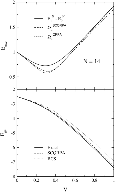
Figure 5: As in Fig.1 but for $N=14$.

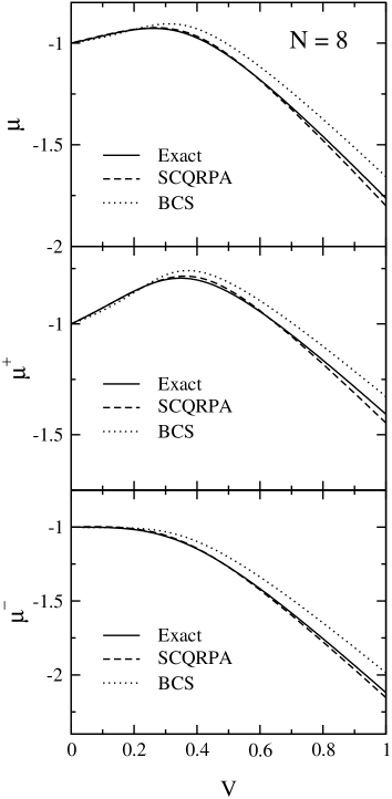
Figure 10: As in Fig.9 but for $N=8$.

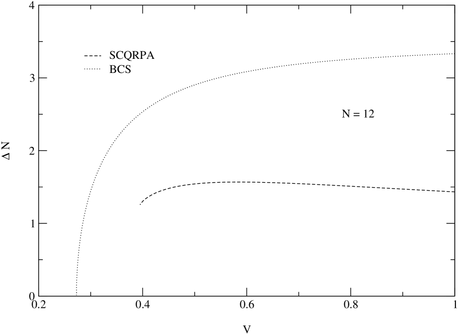
Figure 15: As in Fig.14 but $N=12$.

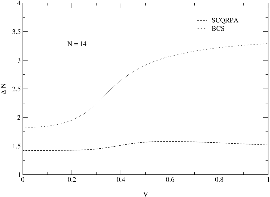
Figure 16: As in Fig.14 but $N=14$.

References

(1)
J. W. Clark, C. G. Källman, C. H. Yang, D. A. Chakka Lakal, Phys. Lett. B 61, 331 (1976);
K. E. Schmidt, V. R. Pandharipande, Phys. Rev. Lett. B 87, 11 (1978);
A. D. Jackson, E. Krotschek, D. E. Metner, R. A. Smith, Nucl. Phys. A 368, 125 (1982);
S. Fantoni, Phys. Rev. B 29, 2544 (1984).
(2)
B. E. Vonderfecht, W. H. Dickhoff, A. Polls, A. Ramos, Nucl. Phys. A 555, 1 (1993);
A. Polls, A. Ramos, J. Ventura, S. Amari, W. H. Dickhoff, Phys. Rev. C 49 3050 (1994).
(3)
T. L. Ainsworth, J. Wambach, D. Pines, Phys. Lett. B 222, 173 (1989);
H. -J. Schulze, J. Cugnon, A. Lejeune, M. Baldo and U. Lombardo, Phys. Lett. B 375, 1 (1996);
U. Lombardo, P. Schuck, W. Zuo, Phys. Rev. C 64, 021301 (2001).
(4)
H. Kucharck, P. Ring, P. Schuck, R. Bengtsson, M. Girod, Phys. Lett. B 216, 249 (1989);
G. Röpke, A. Schnell, P. Schuck and U. Lombardo, Phys. Rev. C 61, 024306 (2000).
(5)
E. Garrido, P. Sarriguren, E. Moya de Guerra, U. Lombardo, P. Schuck, H. -J.
Schulze, Phys. Rev. C 63, 037304 (2001);
(6)
P. Schuck, Z. Physik 241, 395 (1971);
P. Schuck, S. Ethofer, Nucl. Phys. A212, 269 (1973).
(7)
J. Dukelsky, P. Schuck, Phys. Lett. B464, 164 (1999).
(8)
J. G. Hirsch, A. Mariano, J. Dukelsky, P. Schuck,
Ann. Phys. 296, 187 (2002).
(11)
G. Röpke, T. Seifert, H. Stolz, R. Zimmermann, Phys. Stat. Sol. (b)100, 215 (1980);
G. Röpke, Ann. Physik (Leipzig) 3, 145 (1994);
G. Röpke, Z. Phys. B99, 83 (1995).
(12)
P. Krüger, P. Schuck, Europhys. Lett. 72, 395 (1994).
(13)
J. Dukelsky, P. Schuck, Nucl. Phys. A512, 466 (1990).
(14)
J. Dukelsky, P. Schuck, Phys. Lett. B387, 233 (1996).
(15)
J. Dukelsky, G. Röpke, P. Schuck, Nucl. Phys. A628, 17 (1998).
(16)
D. Karadjov, V.V. Voronov, F. Catara, Phys. Lett. B306, 197 (1993);
F. Catara, N. Dinh Dang, M. Sambataro, Nucl. Phys. A579, 1 (1994);
J. Toivanen, J. Suhonen, Phys. Rev. Lett. 75, 410 (1995);
F. Catara, G. Piccitto, M. Sambataro, N. Van Giai, Phys. Rev. B54, 17536 (1996);
J. G. Hirsch, P.O. Hess, O. Civitarese, Phys. Lett. B390, 36 (1997);
F. Krmpotić, T. T. S. Kuo, A. Mariano, E. J. V. de Passos and A. F. R. de Toledo Piza,
Nucl. Phys. A612, 223 (1997).
(17)
R. W. Richardson, Phys. Rev. 141, 949 (1966).
(18)
J. Högaasen-Feldman, Nucl. Phys. 28, 258 (1961);
O. Johns, Nucl. Phys. A 154, 65 (1970).
(19)
M. Baranger, Nucl. Phys. 149, 225 (1970).
(20)
J. Dukelsky, P. Schuck, Mod. Phys. Lett. A 6, 2429 (1991).
(21)
G. Schalow, M. Yamamura, Nucl. Phys. A 161, 93 (1971);
M. Yamamura, Prog. Theo. Phys. 52, 538 (1974);
S. Nishiyama, Prog. Theo. Phys. 55, 1146 (1976).
(22)
B. Feucht, report of training course in Master of Physics , title : Self-Consistent description of quantal fluctuations in a simple model,
June 2000, ISN-Grenoble, Université Joseph Fourier, Grenoble, France.
(23)
M. Sambataro, N. Dinh Dang, Phys. Rev. C 59, 1422 (1999).
(24)
K. Hagino, G.F. Bertsch, Nucl.Phys. A679, 163 (2000).
(25)
P. Ring and P. Schuck, The Nuclear Many-Body Problem (Springer, New York, 1980).
(26)
T. Bertrand, P. Schuck, G. Chanfray, Z. Aouissat, J. Dukelsky, Phys. Rev. C 63, 024301 (2001).
(27)
C. Guet, S. Blundell, Surface Review and Letters 3, 395 (1996).
(28)
E. J. V. de Passos, A. F. R. de Toledo Piza, F. Krmpotić, Phys. Rev. C 58, 1841 (1998).
(29)
H. J. Lipkin, Ann. Phys. (New York) 12, 425 (1960);
Y. Nogami, Phys Rev. 134, B313 (1964).
(30)
J. von Delft, Ann. Phys. (Leipzig) 10, 219 (2001).
(31)
D. Delion, J. Dukelsky, P. Schuck, to be published.