Lorentz Boosted NN Potential for Few-Body Systems:
Application to the three-nucleon bound state

Abstract

A Lorentz boosted two-nucleon potential is introduced in the context of equal time relativistic quantum mechanics. The dynamical input for the boosted nucleon-nucleon (NN) potential is based on realistic NN potentials, which by a suitable scaling of the momenta are transformed into NN potentials belonging to a relativistic two-nucleon Schrödinger equation in the c.m. system. This resulting Lorentz boosted potential is consistent with a previously introduced boosted two-body $t$-matrix. It is applied in relativistic Faddeev equations for the three-nucleon bound state to calculate the ³H binding energy. Like in previous calculations the boost effects for the two-body subsystems are repulsive and lower the binding energy.

I Introduction

Modern realistic nucleon-nucleon (NN) potentials using a sufficiently large number of parameters describe current NN phase shifts very well. The most prominent ones are CD-Bonn[1], Nijmegen 93, I,II [2], and Argonne AV18 [3]. They predict NN observables up to about 350 MeV nucleon laboratory energy perfectly well with a $\chi^{2}/N_{data}\sim 1$. This potential description is linked to a nonrelativistic Schrödinger equation. Converged, nonrelativistic three-nucleon bound state calculations based upon these potentials give values for the triton binding energy between 8.0 and 7.6 MeV [4, 5, 6], whereas the experimental result is 8.48 MeV. There is some sensitivity to nonlocalities in the NN interactions, which influences the value of the triton binding energy. While the Nijmegen 93 and I and the AV18 potential are local, Nijmegen II and CD-Bonn incorporate nonlocalities either via a $p^{2}$ dependence or the nonlocality structure given by Dirac spinors and so-called ‘minimal relativity’ factors. It is well established by now that the purely local interactions in the above list lead to a triton binding energy of about 7.7 MeV, leaving about 0.8 MeV unexplained.

In general, the missing binding energy is attributed to some combination of nonlocality in the NN interactions, three-nucleon force effects and relativistic effects. Of course, these effects are often intermingled, i.e. relativity can motivate specific nonlocalities, and negative energy components of a nucleon wave function could be viewed as a specific subset of three-nucleon forces [7].

The estimation of relativistic effects on the binding of three nucleons has been the focus of a lot of work. However, up to now there has not been reached closure even on the sign of

a relativistic contribution to the three-nucleon binding energy. There are essentially two different approaches to a relativistic three-nucleon bound state calculation, one is a manifestly covariant scheme linked to a field theoretical approach, the other one is based on relativistic quantum mechanics on space-like hypersurfaces (including the light front) in Minkowski space. Within the first scheme Rupp and Tjon [8] find attractive corrections to the triton binding energy, using separable interactions to facilitate the solution of the Bethe-Salpeter-Faddeev equations. A three-dimensional reduction of this equation also finds attractive contributions [9]. The calculations of Stadler et al. [10] are based on a relativistic three-nucleon equation, incorporate the effects of Dirac spinors and include negative energy components. They also incorporate off-shell effects of the negative energy components of the Dirac spinors, and by varying this part, which is not constraint by on-shell NN data, they can achieve an attractive contribution to fit the experimental value. Within the second scheme the relativistic Hamiltonian consists of relativistic kinetic energies, two- and many-body interactions including their boost corrections. The boost corrections are dictated by the Poincaré algebra [11, 12, 13]. There exist already applications for the three-nucleon bound state [14, 15], which suggest a repulsive contribution to the three-nucleon binding. Thus, the relativistic effects found in the two schemes appear controversial, in the approach based on field theory, relativistic effects increase the triton binding energy, in the approach based on relativistic Hamiltonians, relativistic effects decrease the triton binding energy.

To the best of our knowledge we are not aware of any three-nucleon (3N) scattering calculation including relativity in one or the other scheme due to the increased difficulty of a scattering calculation. In order to extend the Hamiltonian scheme in equal time formulation to 3N scattering it would be a very convenient starting point to have the Lorentz boosted NN potential which generates the NN $t$-matrix in a moving frame via a standard Lippmann-Schwinger equation. In this paper we work out the NN potential in an arbitrary frame, and thus place our work in the scheme based on relativistic quantum mechanics. As application of our Lorentz-boosted potential we restrict ourselves to the calculation of the triton binding energy.

The starting point for an NN potential in an arbitrary moving frame is the interaction in the two-nucleon c.m. system, which enters a relativistic NN Schrödinger or Lippmann-Schwinger equation. While realistic NN potentials are defined and fitted in the context of the nonrelativistic Schrödinger equation, NN potentials refitted with the same accuracy in the framework of the relativistic NN Schrödinger equation do not yet exist. A first step in that direction has been done in Ref. [14], where the AV18 potential has been refitted to describe NN phase shifts in the relativistic context. Here we prefer to use a different route and employ an analytical scale transformation of momenta which relates NN potentials in the nonrelativistic and relativistic Schrödinger equations such that exactly the same NN phase shifts are obtained by both equations [16]. Though this transformation is not a substitute for a NN potential with proper relativistic features and though it suffers from some conceptual defects [17], it can serve the purpose of this work, namely to illustrate the effects of a Lorentz boosts on NN potentials.

This paper is organized as follows. In Section II we derive and explicitly formulate the Lorentz-boosted potential related to a given nonrelativistic potential. In Section III we apply our formulation to the Reid Soft Core potential and discuss features of the Lorentz boost. Then we solve the relativistic 3N Faddeev equation based on that Lorentz-boosted potential. We end with a brief summary and outlook in section IV.

II Derivation of the Boosted Potential

A formalism for treating the relativistic three-body Faddeev equations has been introduced in [15]. There a Lorentz boosted t-matrix is constructed from the relativistic two-nucleon $t$-matrix given in the nucleon-nucleon (NN) center-of-mass (c.m.) system. The NN t-matrix obeys the relativistic Lippmann-Schwinger equation:

$$t(\vec{k},\vec{k}_{0})=v(\vec{k},\vec{k}_{0})+\int d^{3}k^{\prime}{{v(\vec{k},\vec{k}^{\prime})~{}t(\vec{k}^{\prime},\vec{k}_{0})}\over{\omega(\vec{k}_{0})-\omega(\vec{k}^{\prime})+i\epsilon}},$$ (1)

where $v(\vec{k},\vec{k}^{\prime})$ is the relativistic potential given in the c.m. system with $\vec{k}$ and $-\vec{k}$ the individual momenta in that system and $\omega(\vec{k})=2\sqrt{k^{2}+m^{2}}$. In Ref. [15] a boosted potential two-nucleon potential $V$ (Eq. (3.4) of [15]) is naturally introduced as

$$V\equiv\sqrt{[\omega(\vec{k})+v]^{2}+{\vec{p}~{}}^{2}}-\sqrt{\omega(\vec{k})^{2}+{\vec{p}~{}}^{2}},$$ (2)

where $\vec{p}$ is the total momentum of the two-nucleon system. Obviously, for $\vec{p}=0$ one obtains $V=v$. For any application to the three-nucleon system, one needs to be able to calculate the matrix elements of $V$ explicitly. Thus we need an explicit representation and use a momentum space form based on eigenstates of the c.m. momentum operator $\vec{k}$ to obtain the matrix elements

$$\langle\vec{k}|V(\vec{p})|\vec{k}^{\prime}\rangle=\langle\vec{k}|\sqrt{[\omega(k)+v]^{2}+{p}^{2}}|\vec{k}^{\prime}\rangle-\langle\vec{k}|\sqrt{\omega(k)^{2}+{p}^{2}}|\vec{k}^{\prime}\rangle.$$ (3)

With the help of the eigenstates $\psi_{b}$ and $|\vec{k}\rangle^{(+)}$ (bound and scattering eigenstates) of the c.m. Hamiltonian ($\omega(k)+v$) the completeness relation is given as

$${\bf 1}=|\psi_{b}\rangle\langle\psi_{b}|+\int|\vec{k}\rangle^{(+)}~{}d^{3}k~{}^{(+)}\langle\vec{k}|.$$ (4)

Inserting the completeness relation into Eq. (3) leads to

$$\langle\vec{k}|V(\vec{p})|\vec{k}^{\prime}\rangle =$$ (7)

$$\langle\vec{k}|\psi_{b}\rangle\langle\psi_{b}|\vec{k}^{\prime}\rangle\sqrt{M_{b}^{2}+p^{2}}+\int d^{3}k^{\prime\prime}\langle\vec{k}|\vec{k}^{\prime\prime}\rangle^{(+)}\sqrt{\omega(k^{\prime\prime})^{2}+\vec{p}^{2}}\;^{(+)}\langle\vec{k}^{\prime\prime}|\vec{k}^{\prime}\rangle$$

$$-\delta(\vec{k}-\vec{k}^{\prime})\sqrt{\omega(k)^{2}+\vec{p}^{2}},$$

where $M_{b}$ is the bound state mass. Using the standard relation between scattering states and plane wave states

$$|\vec{k}\rangle^{(+)}=|\vec{k}\rangle+G_{0}^{(+)}t|\vec{k}\rangle,$$ (8)

the potential matrix element from Eq. (7) can be rewritten as

$$\langle\vec{k}|V(\vec{p})|\vec{k}^{\prime}\rangle$$ (9)

$$= \psi_{b}(\vec{k})\;\sqrt{M_{b}^{2}+p^{2}}\;\psi_{b}(\vec{k}^{\prime})$$ (12)

$$+{{t^{*}(\vec{k}^{\prime},\vec{k};\omega)}\over{\omega-\omega^{\prime}-i\epsilon}}\sqrt{\omega^{2}+p^{2}}+{{t(\vec{k},\vec{k}^{\prime};\omega^{\prime})}\over{\omega^{\prime}-\omega+i\epsilon}}\sqrt{{\omega^{\prime}}^{2}+p^{2}}$$

$$+\int d^{3}k^{\prime\prime}{{t(\vec{k},\vec{k}^{\prime\prime};\omega^{\prime\prime})}\over{\omega^{\prime\prime}-\omega+i\epsilon}}\;\sqrt{{\omega^{\prime\prime}}^{2}+p^{2}}\;{{t^{*}(\vec{k}^{\prime},\vec{k}^{\prime\prime};\omega^{\prime\prime})}\over{\omega^{\prime\prime}-\omega^{\prime}-i\epsilon}}$$

$$= v(\vec{k},\vec{k}^{\prime})+\psi_{b}(\vec{k})(\sqrt{M_{b}^{2}+p^{2}}-M_{b})\psi_{b}(\vec{k}^{\prime})$$ (17)

$$+{1\over{\omega-\omega^{\prime}}}\biggm{[}(\sqrt{\omega^{2}+p^{2}}-\omega)\;\Re[t(\vec{k}^{\prime},\vec{k};\omega)]-(\sqrt{\omega^{\prime 2}+p^{2}}-\omega^{\prime})\;\Re[t(\vec{k},\vec{k}^{\prime};\omega^{\prime})]\biggm{]}$$

$$+{1\over{\omega-\omega^{\prime}}}\Biggm{[}{\cal P}\int d^{3}k^{\prime\prime}{(\sqrt{{\omega^{\prime\prime}}^{2}+p^{2}}-\omega^{\prime\prime})\over{{\omega^{\prime\prime}-\omega}}}t(\vec{k},\vec{k}^{\prime\prime};\omega^{\prime\prime})t^{*}(\vec{k}^{\prime},\vec{k}^{\prime\prime};\omega^{\prime\prime})$$

$$-{\cal P}\int d^{3}k^{\prime\prime}{(\sqrt{{\omega^{\prime\prime}}^{2}+p^{2}}-\omega^{\prime\prime})\over{\omega^{\prime\prime}-\omega^{\prime}}}t(\vec{k},\vec{k}^{\prime\prime};\omega^{\prime\prime})t^{*}(\vec{k}^{\prime},\vec{k}^{\prime\prime};\omega^{\prime\prime})\Biggm{]}.$$

Here ${\cal P}$ denotes the principal value prescription, and $\omega^{\prime}=2\sqrt{{k^{\prime}}^{2}+m^{2}}$, and $\omega^{\prime\prime}=2\sqrt{{k^{\prime\prime}}^{2}+m^{2}}$. Note that the matrix elements is well defined for $\omega=\omega^{\prime}$, since both brackets vanish in this case.

Thus, the boosted potential, which depends on the total two-nucleon momentum $\vec{p}$, requires the knowledge of the NN bound state wave function and the half-shell NN $t$-matrices given in the 2N c.m. system. For any given potential $v$ those quantities can be calculated by standard methods. Once the matrix elements $\langle\vec{k}|V(\vec{p})|\vec{k}^{\prime}\rangle\equiv V(\vec{k},\vec{k}^{\prime};p)$ are known, the boosted $t$-matrix elements $T\equiv T(\vec{k},\vec{k}^{\prime};p)$ can be calculated from the relativistic Lippmann-Schwinger equation,

$$T(\vec{k},\vec{k^{\prime}};\vec{p})=V(\vec{k},\vec{k^{\prime}};\vec{p})+\int d^{3}k^{\prime\prime}{V(\vec{k},\vec{k^{\prime\prime}};\vec{p})T(\vec{k}^{\prime\prime},\vec{k^{\prime}};\vec{p})\over{\sqrt{{\omega^{\prime}}^{2}+p^{2}}-\sqrt{{\omega^{\prime\prime}}^{2}+p^{2}}+i\epsilon}}.$$ (18)

For any given momentum $\vec{p}$ the bound state wave function $\psi_{b}$ defined in the c.m. system obeys

$$\psi_{b}(\vec{k})={1\over{\sqrt{M_{b}^{2}+p^{2}}-\sqrt{{\omega}^{2}+p^{2}}}}\int d^{3}k^{\prime}V(\vec{k},\vec{k^{\prime}};\vec{p})\psi_{b}(\vec{k^{\prime}}).$$ (19)

This eigenvalue equation is an excellent numerical test for the numerical calculation of the boosted potential, since it has to reproduce exactly the boosted energy $\sqrt{M_{b}^{2}+p^{2}}$ of a deuteron in motion.

In Ref. [15] the Lorentz boosted $T$-matrix was already introduced but calculated in a different fashion (see Eq.(3.27) therein). In the procedure we suggest here, we want to focus on the calculation of the boosted potential. We want to remark that despite the occurrence of complex valued half-shell t-matrices in Eq. (9) the potential matrix element $V(\vec{k},\vec{k^{\prime\prime}};\vec{p})$ is real. The proof is given in Appendix A. As a consequence of that and the manifest symmetry of $\langle\vec{k}|V(\vec{p})|\vec{k}^{\prime}\rangle$ it folows from Eq. (18) that one can define an unitary S-matrix. We define the S-matrix as

$$S(\vec{k},\vec{k^{\prime}};\vec{p})\equiv{4\over{k\sqrt{\omega^{2}+p^{2}}}}\;\delta(\sqrt{\omega^{2}+p^{2}}-\sqrt{{\omega^{\prime}}^{2}+p^{2}})\hat{S}(\vec{k},\vec{k^{\prime}};\vec{p}),$$ (20)

with

$$\hat{S}(\vec{k},\vec{k^{\prime}};\vec{p})\equiv\delta(\hat{k}-\hat{k^{\prime}})-2i\pi{k\sqrt{\omega^{2}+p^{2}}\over 4}\;T(\vec{k},\vec{k^{\prime}};\vec{p}).$$ (21)

Then one can show in the standard way that

$$\int d\hat{k^{\prime\prime}}\hat{S}(\vec{k},\vec{k^{\prime\prime}};\vec{p})\hat{S}^{*}(\vec{k}^{\prime},\vec{k^{\prime\prime}};\vec{p})=\delta(\hat{k}-\hat{k^{\prime}}).$$ (22)

Note that $\vec{k}=k\hat{k}$, $\vec{k^{\prime\prime}}=k\hat{k^{\prime\prime}}$, and $\vec{k^{\prime}}=k\hat{k^{\prime}}$, where the quantities $\hat{k}$, $\hat{k^{\prime}}$, and $\hat{k^{\prime\prime}}$ are unit vectors.

III Applications

In this section we would like to consider the Lorentz boosted potential and use it to calculate the binding energy of the triton.

A Calculation of the boosted potential

First we need to construct a suitable potential which enters the relativistic Lippmann Schwinger equation, Eq. (1). A standard nonrelativistic potential fulfills the nonrelativistic Lippmann Schwinger equation for the nonrelativistic t-matrix $t^{(nr)}$,

$$t^{(nr)}(\vec{q},\vec{q^{\prime}})=v^{(nr)}(\vec{q},\vec{q^{\prime}})+\int d^{3}q^{\prime\prime}{{v^{(nr)}(\vec{q},\vec{q^{\prime\prime}})\;t^{(nr)}(\vec{q^{\prime\prime}},\vec{q^{\prime}})}\over{{\vec{q^{\prime}}^{2}\over m}-{{\vec{q^{\prime\prime}}}^{2}\over m}+i\epsilon}}.$$ (23)

Using a relativistic propagator in Eq. (23) will not result in the same phase shifts or observables. However, there is a scale transformation, which generates a phase equivalent relativistic potential $v$ from a nonrelativistic potential $v^{(nr)}$ [16]. This scale transformation is derived from requiring that the relativistic and nonrelativistic form of the kinetic energy give the same result. This requirement leads to analytic relations connecting the nonrelativistic momentum $q$ with the corresponding relativistic momentum $k$,

$$q\buildrel!\over{\equiv}\sqrt{m}\sqrt{\omega({\vec{k}})-2m}.$$ (24)

The details of the derivation are given in Ref. [16]. Here we only list the results necessary for the understanding of our present considerations. For a given nonrelativistic potential $v^{(nr)}(\vec{q},\vec{q^{\prime}})$ the corresponding phase equivalent relativistic potential is obtained as

$$v(\vec{k},\vec{k^{\prime}})={1\over h(q)}v^{(nr)}(\vec{q},\vec{q^{\prime}}){1\over h(q^{\prime})}.$$ (25)

The corresponding relativistic NN t-matrix can be obtained from the nonrelativistic one in a similar fashion,

$$t(\vec{k},\vec{k^{\prime}};\omega^{\prime})={1\over h(q)}~{}t^{(nr)}(\vec{q},\vec{q^{\prime}}){1\over h(q^{\prime})}.$$ (26)

The Jacobian function $h(q)$ is defined as

$$h(q)\equiv\sqrt{(1+{q^{2}\over 2m^{2}})\sqrt{1+{q^{2}\over 4m^{2}}}}.$$ (27)

The results of Eqs.(25) and (26) can be derived from the scale transformation of Eq. (24). Of course, they are not equivalent to the introduction of a relativistic potential $v$ and a corresponding NN t-matrix based on a field theory theory. However, for our purposes, the scale transformation is a very useful and simple parameterization of a relativistic NN potential, which conserve the NN phase shifts exactly, and which can enter Eq. (2) for the boosted potential. We want to remark here, that Eq. (2) is general and independent of the way, the relativistic potential was obtained.

In order to study the effect of the boost on the potential in more detail, we choose as the nonrelativistic potential the Reid soft core potential (RSC) [18]. The RSC potential in the ${}^{1}S_{0}$ state is given by

$$v^{(nr)}(r)=(-10.463{e^{-\mu r}\over\mu r}-1650.6{e^{-4\mu r}\over\mu r}+6484.2{e^{-7\mu r}\over\mu r})~{}~{}{\rm MeV}$$ (28)

where $\mu$ is 0.7 fm^-1.

In Fig. 1 a contour plot of $v^{(nr)}(q,q^{\prime})$ is given for the ${}^{1}S_{0}$ state. It should be noted that this particular potential is positive for all values of $q$ and $q^{\prime}$. Next, we successively apply first the scale transformation and then the boost to $v^{(nr)}(q,q^{\prime})$. In Fig. 2 we compare the projections on the ${}^{1}S_{0}$ state of the three potential functions, namely $v^{(nr)}(\vec{q},\vec{q}^{\prime})$, $v(\vec{k},\vec{k}^{\prime})$, and $V(\vec{k},\vec{k^{\prime}};\vec{p})$ as a function of $k$. Since the scale transformation of Eq. (24) changes the momentum scale, we express $v^{(nr)}(\vec{q},\vec{q}^{\prime})$ in terms of $k$ and $k^{\prime}$, in order to compare it with the other two potential functions. We choose two fixed values for $k^{\prime}$, namely $k^{\prime}$=1 fm^-1 and $k^{\prime}$=15 fm^-1. The total two-nucleon momentum is chosen as $p$=20 fm^-1. First, we would like to make some more general remarks. For small momenta $q$, i.e. in a very nonrelativistic regime, on has $q\approx$ $k$. Furthermore, since the function $h(q)$ is always larger than 1, $v$ will be always smaller than $v^{(nr)}$. At larger momenta $q$ differs from $k$ and the relation between $v$ and $v^{(nr)}$ depends in general on the shape of $v$. In our case $v$ is always smaller than $v^{(nr)}$. The boost effect leads to another overall decrease of the values of $V$ except for small momenta, where $V$ is larger than $v$ and $v^{(nr)}$. We also want to point out that we chose quite a large two-nucleon momentum $p$ in order to show the effects of the boost. For two-nucleon momenta in the order of about 5 fm^-1, the boost effects are much smaller. In fact, almost all of the difference between $v$ and $v^{(nr)}$ would be given by the scale transformation, i.e. by an underlying different scattering equation.

B Calculation of the triton binding energy

Now let us move on to entering the boosted NN potential into the relativistic three-body Faddeev equation to calculate the bound state of ³H. The relativistic Faddeev equation as already introduced in Ref. [15] reads

$$\phi(\vec{k},\vec{p})={1\over E_{b}-{\cal E}(\vec{k},\vec{p})}\int d^{3}p^{\prime}{T_{a}(\vec{k},\vec{\kappa}(\vec{p^{\prime}},-\vec{p}-\vec{p^{\prime}});\vec{p})\over{{\cal N}(\vec{p^{\prime}},-\vec{p}-\vec{p^{\prime}}){\cal N}(-\vec{p}-\vec{p^{\prime}},\vec{p})}}\;\phi(\vec{\kappa}(-\vec{p}-\vec{p^{\prime}},\vec{p}),\vec{p^{\prime}})$$ (29)

where $\phi$ is the Faddeev component and $E_{b}$ the three-body binding energy. The index $a$ at the boosted T-matrix indicates a properly antisymmetrized two-body T-matrix. The vector $\vec{k}$ represents the relative momentum in the two-body c.m. subsystem as in the nonrelativistic case, and $\vec{p}$ stands for the momentum of the corresponding third particle. At the same time $\vec{p}$ is the (negative) total momentum of the two-body subsystem and thus is responsible for the boosts of that subsystem. Clearly, the three individual nucleon momenta sum up to zero. If $\vec{p}$ and $\vec{p^{\prime}}$ are the momenta of two individual nucleons, then their relative momentum (half the momentum difference) in their c.m. system is obtained through a Lorentz transformation, which is explicitly given as

$$\vec{\kappa}(\vec{p},\vec{p^{\prime}})\equiv{1\over 2}\left[\vec{p}-\vec{p^{\prime}}-(\vec{p}+\vec{p^{\prime}}){\Omega-\Omega^{\prime}\over(\Omega+\Omega^{\prime})+\sqrt{(\Omega+\Omega^{\prime})^{2}-(\vec{p}+\vec{p^{\prime}})^{2}}}\right],$$ (30)

where $\Omega(p)=\sqrt{m^{2}+{p}^{2}}=\Omega$ and $\Omega^{\prime}=\sqrt{m^{2}+{p^{\prime}}^{2}}$. The last term in Eq. (3.8) reflects the relativistic effect in the definition of a relative momentum. When going from individual momenta $\vec{p}$ and $\vec{p^{\prime}}$ of the subsystem to the relative momentum and the total two-body momentum $\vec{p}+\vec{p^{\prime}}$ one has to consider the Jacobian of that transformation. The square root of the Jacobian is given by [15]

$${\cal N}(\vec{p},\vec{p^{\prime}}) = \left[\left|{\partial(\vec{p},\vec{p^{\prime}})\over\partial(\vec{k},\vec{p}+\vec{p^{\prime}})}\right|\right]^{1/2}$$ (31)

$$= \left[4\Omega\Omega^{\prime}\over{\sqrt{(\Omega+\Omega^{\prime})^{2}-(\vec{p}+\vec{p^{\prime}})^{2}}(\Omega+\Omega^{\prime})}\right]^{1/2}.$$ (32)

The kinetic energy ${\cal E}$ is given by

$${\cal E}(\vec{k},\vec{p}) = \sqrt{\omega^{2}(k)+m^{2}}+\Omega-3m$$ (33)

$$= \Omega+\Omega^{\prime}+\Omega^{\prime\prime}-3m.$$ (34)

A detailed derivation of the above relations is given in Ref. [15].

In our calculation of the triton binding energy the relativistic Faddeev equation, Eq. (29) is solved in a partial wave basis. The explicit representation of Eq. (29) in a partial wave decomposition is given in Appendix B. Since we are here only interested to test the feasibility of our approach, we only perform a 5-channel calculation at present. This means we allow the NN forces to act only in the states ${}^{1}S_{0}$ and ${}^{3}S_{1}-^{3}D_{1}$ (see e.g. table 3.4 in [20]). We want to point out that in contrast to a nonrelativistic calculation not only the Faddeev component and the T-matrix depend on the angle between $\vec{p}$ and $\vec{p^{\prime}}$ but also the Jacobian $\cal N$. In this first approach we ignore the Lorentz transformation of the spins states. As NN potentials we employ the high-precision potentials CD-Bonn [1], NijmI,II, 93 [2], and AV18[3], as well as the Reid Soft Core potential [18] and two different Yamaguchi [21] potentials. For all potentials (with the exception of RSC) we use np forces only. With those potentials given, our calculation proceeds as follows. First, we perform the scale transformation of Eq. (24) to obtain a phase equivalent potential obeying the relativistic two-body Lippmann-Schwinger equation. Then we boost this potential and solve for the relativistic, boosted T-matrix, which enters the relativistic Faddeev equation, Eq. (29). This is in contrast to the approach given in Ref. [15] where a relativistic NN t-matrix in the NN c.m. frame was calculated first, and this t-matrix was boosted to the obtain the T-matrix entering Eq. (29). We also want to point out that the relativistic potential used in Ref. [15] is only approximately phase shift equivalent to the nonrelativistic one.

Our results for the relativistic Faddeev calculations based on five channels are displayed in Table I. For comparison, we also list the binding energies $E_{b}^{(nr)}$ obtained from a nonrelativistic five channel calculation. We want to emphasize that the underlying relativistic and nonrelativistic NN forces are strictly phase equivalent and give the same deuteron binding energy. Only under these conditions it is reasonable to pin down relativistic effects in the triton binding energy. From Table I we see that the difference between the relativistic and nonrelativistic binding energies span a range of about 0.29-0.43 MeV. The Yamaguchi potentials do not fall into this range. From Table I we can conclude that the relativistically calculated triton binding energy is reduced in magnitude compared to the one calculated nonrelativistically. A related investigation was carried out in Ref. [14] based on the AV18 potential. There the nonrelativistic NN potential was augmented by relativistic corrections of low orders following the work of [12] and was refitted to the NN phase shifts. The final relativistic correction to the binding energy of ³H given in Ref. [14] is 0.33MeV, which is comparable to our present findings. It is interesting to notice, that in the case of the Yamaguchi potentials, which are purely attractive, the relativistic, repulsive effect is weaker, namely only about 0.2 MeV. This is presumably connected to the absence of short range repulsive force components, i.e. high momentum components, which are presumably mostly affected by the relativistic effects. However, it will be difficult to provide general arguments on the relative size of the relativistic effects under consideration, since they most likely depend on the specific functional form of the potential. We also want to mention, that for nonrelativistic calculations the contributions of the higher partial waves in the two-body subsystem are attractive and range from about 0.04 to 0.24 MeV.

In order to shed some more light on the different contributions to our relativistic calculation, we want to expose the effect of the normalization factor separately. To do so, we solve Eq. (29) under the assumption that ${\cal N}=1$, which is the nonrelativistic limit of that quantity. The resulting binding energies are listed in the last column of Table I. replaced by 1, which is the nonrelativistic limit of that quantity. We see that $\cal N$ gives a repulsive contribution in all cases.

Finally we display the relativistic and nonrelativistic Faddeev components in Figs. 3 and 4. We choose the channel related to the two-body state ${}^{1}S_{0}$, which is one of the five channels. The figures show that the relativistic Faddeev component is more extended into the high $k$-region than the nonrelativistic one. As a reminder, the corresponding two-body relative momentum is denoted by $q$, see Eq. (24). However, when the momentum $k$ of the relativistic Faddeev component is expressed in terms of $q$ according to Eq. (24) and the component is replotted as a function of $q$, then the shape of this Faddeev component is very close to the nonrelativistic one, as shown in Fig. 5.

IV Summary and Outlook

We derived and presented an explicit expression for a Lorentz boosted NN potential, which can be used to determine the two-body T- matrix in a frame, in which the total momentum of the two particles is different from zero. The description of two-body systems with non-zero total momentum is relevant for calculating properties in an interacting three-body system in a relativistic framework. The general T-matrix was inserted into a relativistic three-body Faddeev equation for the bound state, which was proposed in [15]. The dynamical input consisted of NN potentials used in a relativistic two-body Schrödinger equation which are exactly phase equivalent to nonrelativistic NN potentials used in the nonrelativistic Schrödinger equation. The phase equivalence of the two different NN potentials is achieved by a momentum scale transformation [16]. We applied this scheme to various modern high precision NN potentials and compared resulting three-nucleon binding energies from the nonrelativistic and relativistic 3N Faddeev equations. In all case the relativistic effects turned out to be repulsive and of the order of 400 keV.

The effect of the boost turns out to be relatively small for moderate total momenta of the two nucleons, however at high momenta they are quite visible. If one compares the relativistic and nonrelativistic Faddeev components one notices some enhancement for high momentum components in the two-body subsystem.

The access to boosted NN potentials opens the door to considering the relativistic Faddeev equations for three-nucleon scattering. The need for a relativistic description of three-nucleon scattering became already apparent when measurements of the total cross section for neutron-deuteron scattering [22] were analyzed within the framework of nonrelativistic Faddeev calculations [23]. Here, NN forces alone were not sufficient to describe the data above about 100 MeV. The discrepancy is most likely due to missing corrections from three-nucleon forces and relativistic effects. The relativistic corrections considered in Ref. [23] were only of kinematic nature, but they lead to an increase of the total cross section by about 3% at 100 MeV and about 7% at 250 MeV. This estimate, though very crude, emphasizes the importance of a consistent treatment of relativistic effects especially in scattering. The availability of a boosted NN potential is one step in that direction. Additional technical steps in relation to the relativistic free 3-body propagator and its singularity structure have already been worked out [24]. We expect that the Wigner rotations of the spin states can be performed along the line given in [13].

A Proof of the Reality of the boosted Potential

The boosted potential is given in Eq. (18). Obviously, the first three terms are real. Here we show that the remaining forth term,

$${1\over{\omega-\omega^{\prime}}} \{ {\cal P}\int d^{3}k^{\prime\prime}{(\sqrt{{\omega^{\prime\prime}}^{2}+p^{2}}-\omega^{\prime\prime})\over{{\omega^{\prime\prime}-\omega}}}t(\vec{k},\vec{k}^{\prime\prime};\omega^{\prime\prime})t^{*}(\vec{k}^{\prime},\vec{k}^{\prime\prime};\omega^{\prime\prime})$$ (A1)

$$- {\cal P}\int d^{3}k^{\prime\prime}{(\sqrt{{\omega^{\prime\prime}}^{2}+p^{2}}-\omega^{\prime\prime})\over{\omega^{\prime\prime}-\omega^{\prime}}}t(\vec{k},\vec{k}^{\prime\prime};\omega^{\prime\prime})t^{*}(\vec{k}^{\prime},\vec{k}^{\prime\prime};\omega^{\prime\prime})\}$$ (A2)

is also real. This term contains the complex expression $t(\vec{k},\vec{k}^{\prime\prime};\omega^{\prime\prime})t^{*}(\vec{k}^{\prime},\vec{k}^{\prime\prime};\omega^{\prime\prime})$, which we will have to rewrite in order to show that the integration over it results in a real number. First, we note that only the half-shell t-matrix enters the integration in Eq. (A2). Via the Heitler equation it can be related to the K-matrix,

$$t(\vec{k},\vec{k}^{\prime\prime};\omega^{\prime\prime}) = K(\vec{k},\vec{k}^{\prime\prime};\omega^{\prime\prime})-i\pi\sqrt{{k^{\prime\prime}}^{2}+m^{2}}\>k^{\prime\prime}\int d\hat{k}^{\prime\prime\prime}K(\vec{k},\vec{k}^{\prime\prime\prime};\omega^{\prime\prime})t(\vec{k}^{\prime\prime\prime},\vec{k}^{\prime\prime};\omega^{\prime\prime}),$$ (A3)

where $|\vec{k}^{\prime\prime\prime}|=k^{\prime\prime}$ is on-energy-shell. The K-matrix is real and defined in the standard fashion as

$$K(\vec{k},\vec{k}^{\prime\prime};\omega^{\prime\prime})=v(\vec{k},\vec{k}^{\prime\prime})+{\cal P}\int d^{3}k^{\prime\prime\prime}{v(\vec{k},\vec{k}^{\prime\prime\prime})K(\vec{k}^{\prime\prime\prime},\vec{k}^{\prime\prime};\omega^{\prime\prime})\over{{\omega^{\prime\prime}-\omega^{\prime\prime\prime}}}}$$ (A4)

In order to carry out the angular integration in Eq. (A4), we use the partial wave representations of the t- and K-matrix,

$$t(\vec{k},\vec{k}^{\prime\prime};\omega^{\prime\prime}) = \sum_{lm}t_{l}(k,k^{\prime\prime};\omega^{\prime\prime})Y_{lm}(\hat{k})Y^{*}_{lm}(\hat{k}^{\prime\prime}),$$ (A5)

and

$$K(\vec{k},\vec{k}^{\prime\prime};\omega^{\prime\prime}) = \sum_{lm}K_{l}(k,k^{\prime\prime};\omega^{\prime\prime})Y_{lm}(\hat{k})Y^{*}_{lm}(\hat{k}^{\prime\prime}).$$ (A6)

Inserting these partial wave expressions into Eq. (A4) leads to a partial wave representation of $t$ as

$$t_{l}(k,k^{\prime\prime};\omega^{\prime\prime})=K_{l}(k,k^{\prime\prime};\omega^{\prime\prime})(1-i\pi\sqrt{{k^{\prime\prime}}^{2}+m^{2}}\;k^{\prime\prime}\;t_{l}(k^{\prime\prime},k^{\prime\prime};\omega^{\prime\prime})).$$ (A7)

Thus, the half-shell t-matrix $t_{l}(\vec{k},\vec{k^{\prime\prime}};\omega^{\prime\prime})$ receives its complex parts only from the factor $(1-i\pi\sqrt{{k^{\prime\prime}}^{2}+m^{2}}k^{\prime\prime}t_{l}(k^{\prime\prime},k^{\prime\prime};\omega^{\prime\prime}))$ which does not depend on $k$. Using the partial wave expansions of Eqs. (A5) and (A6) leads to

$$\int d\hat{k}^{\prime\prime}\;t(\vec{k},\vec{k}^{\prime\prime};\omega^{\prime\prime})t^{*}(\vec{k}^{\prime},\vec{k}^{\prime\prime};\omega^{\prime\prime})$$ (A8)

$$= \sum_{lm}t_{l}(k,k^{\prime\prime};\omega^{\prime\prime})t_{l}^{*}(k^{\prime},k^{\prime\prime};\omega^{\prime\prime})Y_{lm}(\hat{k})Y^{*}_{lm}(\hat{k}^{\prime})$$ (A9)

$$= \sum_{l}(2l+1)K_{l}(k,k^{\prime\prime};\omega^{\prime\prime})K_{l}(k^{\prime},k^{\prime\prime};\omega^{\prime\prime})\left(1+\pi^{2}({{k^{\prime\prime}}^{2}+m^{2}}){k^{\prime\prime}}^{2}|t_{l}(k^{\prime\prime},k^{\prime\prime};\omega^{\prime\prime})|^{2}\right)P_{l}(\hat{k}\cdot\hat{k^{\prime}}).$$ (A10)

Here $P_{l}$ is the Legendre polynomial. The expression given in Eq. (A8) is manifestly real and consequently the expression given in Eq. (A2) is real.

B Partial Wave Representation

In a partial wave representation the relativistic Faddeev Eq. (29) is explicitly given as

$$\phi_{\alpha}(k,p) = {1\over E_{b}-{\cal E}(k,p)}\sum_{\alpha^{\prime}\alpha^{\prime\prime}}\int_{0}^{\infty}dp^{\prime}{p^{\prime}}^{2}\int_{-1}^{1}dx{T_{\alpha\alpha^{\prime}}(k,\kappa_{1};p^{\prime})\over{{\kappa_{1}}^{l^{\prime}}}}$$ (B2)

$$\times{G_{\alpha^{\prime}\alpha^{\prime\prime}}(p,p^{\prime},x)\over{{\cal N}_{1}(p,p^{\prime},x){\cal N}_{2}(p,p^{\prime},x)}}{\phi_{\alpha^{\prime\prime}}(\kappa_{2},{p^{\prime}})\over{\kappa_{2}}^{l^{\prime\prime}}}$$

where

$$G_{\alpha\alpha^{\prime}}(p,p^{\prime},x)=\sum_{\cal L}P_{\cal L}(x)\sum_{l_{1}+l_{2}=l}\sum_{l^{\prime}_{1}+l^{\prime}_{2}=l^{\prime}}{\left\{(1+y_{1})p\right\}}^{l_{2}+l^{\prime}_{2}}{\left\{(1+y_{2})p^{\prime}\right\}}^{l_{1}+l^{\prime}_{1}}g_{\alpha\alpha^{\prime}}^{{\cal L}l_{1}l_{2}l^{\prime}_{1}l^{\prime}_{2}},$$ (B3)

and

$$\kappa_{1} = \sqrt{{p^{\prime}}^{2}+{(1+y_{1})^{2}\over 4}{p}^{2}+(1+y_{1})pp^{\prime}x},$$ (B4)

$$\kappa_{2} = \sqrt{{p}^{2}+{(1+y_{2})^{2}\over 4}{p^{\prime}}^{2}+(1+y_{2})pp^{\prime}x},$$ (B5)

and

$$y_{1} = y_{1}(p,p^{\prime},x)$$ (B6)

$$= {\sqrt{m^{2}+{p^{\prime}}^{2}}-\sqrt{m^{2}+p^{2}+{p^{\prime}}^{2}+2pp^{\prime}x}\over{\sqrt{m^{2}+{p^{\prime}}^{2}}+\sqrt{m^{2}+p^{2}+{p^{\prime}}^{2}+2pp^{\prime}x}+\sqrt{(\sqrt{m^{2}+{p^{\prime}}^{2}}+\sqrt{m^{2}+p^{2}+{p^{\prime}}^{2}+2pp^{\prime}x})^{2}-p^{2}}}},$$ (B7)

$$y_{2} = y_{1}(p^{\prime},p,x).$$ (B9)

When explicitly calculating the normalization factor ${\cal N}({{\vec{p}}^{\prime}},-{\vec{p}}-{{\vec{p}}^{\prime}})$, it turns out that ${\cal N}({{\vec{p}}^{\prime}},-{\vec{p}}-{{\vec{p}}^{\prime}})\rightarrow{\cal N}_{1}(p,p^{\prime},x)$ with

$${\cal N}_{1}(p,p^{\prime},x)=$$ (B11)

$$\left(4\sqrt{m^{2}+{p^{\prime}}^{2}}\sqrt{m^{2}+p^{2}+{p^{\prime}}^{2}+2pp^{\prime}x}\over{\sqrt{(\sqrt{m^{2}+{p^{\prime}}^{2}}+\sqrt{m^{2}+p^{2}+{p^{\prime}}^{2}+2pp^{\prime}x})^{2}-p^{2}}(\sqrt{m^{2}+{p^{\prime}}^{2}}+\sqrt{m^{2}+p^{2}+{p^{\prime}}^{2}+2pp^{\prime}x})}\right)^{1/2}.$$

In a similar vain, ${\cal N}(-{\vec{p}}-{\vec{p}^{\prime}},{\vec{p}})\rightarrow{\cal N}_{2}(p,p^{\prime},x)$, with

$${\cal N}_{2}(p,p^{\prime},x)={\cal N}_{1}(p^{\prime},p,x).$$ (B12)

The index $\alpha$ summarizes a set of quantum numbers (channels)

$$|\alpha\rangle=|(ls)j(\lambda{1\over 2})I(jI)J(t{1\over 2})T\rangle,$$ (B13)

where $l,s,j$ and $t$ are orbital angular momentum, total spin, total angular momentum j and total isospin in the two-body subsystem. The indices $\lambda,I$, $J$, and $T$ stand for the orbital angular momentum, the total angular momentum of the third particle, the total three-body angular momentum, and the total isospin [19, 20]). The quantity $g_{\alpha\alpha^{\prime}}^{{\cal L}l_{1}l_{2}l^{\prime}_{1}l^{\prime}_{2}}$ represents the standard permutation operator coefficient.

Finally, when taking the limits

$$y_{1},y_{2} \to 0,$$ (B14)

$${\cal N}_{1},{\cal N}_{2} \to 1,$$ (B15)

one obtains the nonrelativistic result

$${\cal E}(k,p) \to {k^{2}\over m}+{3p^{2}\over 4m},$$ (B16)

$$T \to t^{(nr)},$$ (B17)

and the relativistic Faddeev equation, Eq. (29), reduces to the nonrelativistic one.

interaction	$E_{b}$	$E_{b}^{(nr)}$	$\Delta$	$E_{b}\;({\cal N}\to 1$)
RSC [18]	-6.59	-7.02[25]	0.43	-6.63
CD-Bonn [1]	-7.98	-8.33	0.35	-8.03
Nijmegen II[2]	-7.22	-7.65	0.43	-7.27
Nijmegen I[2]	-7.71	-8.00	0.29	-7.76
Nijmegen 93 [2]	-7.46	-7.76	0.30	-7.51
AV18 [3]	-7.23	-7.66	0.43	-7.27
Yamaguchi I [21]	-9.93	-10.13	0.20	-10.04
Yamaguchi II[21]	-8.30	-8.48	0.18	-8.40
exp.	-8.48

TABLE I.: The relativistic ($E_{b}$) and nonrelativistic ($E_{b}^{(nr)}$) triton binding energies in MeV obtained from different nonrelativistic potentials. The quantity $\Delta$ is defined as $\Delta\equiv E_{b}-E^{(nr)}_{b}$. For comparision we also list the results of the relativistic calculation when the Jacobian function ${\cal N}$ is set to 1.

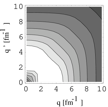
FIG. 1.: Contour plots for the Reid soft core potential $v^{(nr)}(q,q^{\prime})$ in the state ${}^{1}S_{0}$ in momentum space. All values are positive, decreasing from light to darker shades.

FIG. 2.: The nonrelativistic potential $v^{(nr)}(q,q^{\prime})$ (solid line), the scale transformed potential $v(k,k^{\prime})$ (long dashed line) and the boosted potential $V(k,k^{\prime};p)$ (short dashed line) as function of the momentum $k$ and two fixed momenta $k^{\prime}$. All potentials are projected on the ¹S₀ partial wave state. The figure shows two groups of lines: the upper group ( V $>$ 0.6fm^-1 ) is calculated for a fixed $k^{\prime}$=1 fm^-1 and the lower one for a fixed $k^{\prime}$=15 fm^-1. The boosted potential $V(k,k^{\prime};p)$ is evaluated at $p$=20fm^-1.

FIG. 3.: The relativistic Faddeev component $\phi(k,p)$ linked to the ¹S₀ state in the 2-body subsystem.

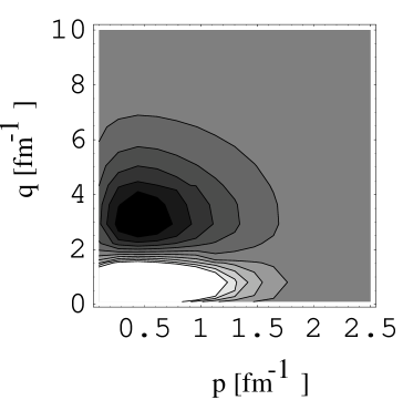
FIG. 4.: The nonrelativistic Faddeev component $\phi(q,p)$ corresponding to Fig. 3. The contour lines carry the same values as in Fig. 3. Note the difference in the 2-nucleon subsystem momentum $q$ to $k$ in Fig. 3.

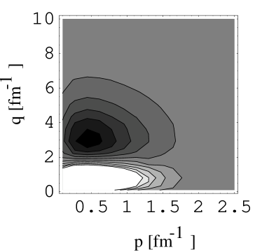
FIG. 5.: The relativistic Faddeev component. From Fig. 3, where $k$ is expressed in terms of $q$. Contour lines are as in Figs. 3 and 4.

REFERENCES

- [1] R. Machleidt et al., Phys. Rev. C 53, R1483 (1996).
- [2] V. G. J. Stoks et al., Phys. Rev. C 49, 2950 (1994).
- [3] R. B. Wiringa et al., Phys. Rev. C 51, 38 (1995).
- [4] J. L. Friar, et al., Phys. Lett. B 311, 4 (1993).
- [5] A. Nogga, D. Hüber, H. Kamada, W. Glöckle, Phys. Lett. B 409, 19 (1997).
- [6] A. Nogga, PhD Thesis, Ruhr-University Bochum, 2001.
- [7] F. Coester, Proceedings to the 11th International Conference on Recent Progress in Many-Body Theories, nucl-th/0111025.
- [8] G. Rupp, J. A. Tjon, Phys. Rev. C 45, 2133 (1992).
- [9] F. Sammarruca, R. Machleidt, Few-Body Syst. 24, 87 (1998).
- [10] A. Stadler, F. Gross, M. Frank, Phys. Rev. C 56, 2396 (1997); A. Stadler, F. Gross, Phys. Rev. Lett. 78, 26 (1997).
- [11] B. Bakamjian, L. H. Thomas, Phys. Rev. 92, 1300 (1952).
- [12] L. L. Foldy, Phys. Rev. 122, 275 (1961); R. A. Krajcik, L. L. Foldy, Phys. Rev. D 10, 1777 (1974).
- [13] B. D. Keister, AIP Conf. Proc. 334, 164 (1995); B. D. Keister, W. N. Polyzou, Adv. Nucl. Phys. 20 , 225 (1991).
- [14] J. Carlson, V. R. Pandharipande, R. Schiavilla, Phys. Rev. C47, 484 (1993); J. L. Forest, V. R. Pandharipande, J. L. Friar, Phys. Rev. C 52 , 568 (1995); J. L. Forest, V. R. Pandharipande, J. Carlson, R. Schiavilla, Phys. Rev. C 52, 576 (1995).
- [15] W. Glöckle, T-S. H. Lee, and F. Coester, Phys. Rev. C 33, 709 (1986); F. Coester, Helv. Phys. Acta 38, 7 (1965); L. Müller, Nucl. Phys. A360, 331 (1981); W. Glöckle, L. Müller, Phys. Rev. C 23, 1183 (1981).
- [16] H. Kamada and W. Glöckle, Phys. Rev. Lett. 80, 2547 (1998).
- [17] T.W. Allen, G.L. Payne, and Wayne N. Polyzou, Phys. Rev. C 62, 054002 (2000).
- [18] R. V. Reid, Ann. Phys. 50 , 411 (1968).
- [19] W. Glöckle, H. Witała, D. Hüber, H. Kamada, J. Golak, Phys. Rep. 274, 107 (1996).
- [20] W. Glöckle, The Quantum-Mechanical Few-Body Problem (Springer Verlag, Berlin, Heiderberg, 1983).
- [21] B. F. Gibson, D. R. Lehman, Phys. Rev. C 14, 685 (1976).
- [22] W. P. Abfalterer et al., Phys. Rev. Lett. 81, 57 (1998).
- [23] H. Witała et al., Phys. Rev. C59, 3035 (1999).
- [24] H. Kamada, Few-Body Syst. Suppl. 12 , 433 (2000).
- [25] W. Glöckle, Nucl. Phys. A 381, 343 (1982); C. Hadjuk, P. U. Sauer, Nucl. Phys. A 369, 321 (1981); I. R. Afnan, N. D. Birrell, Phys. Rev. C 16, 823 (1977).