Explicitly covariant light-front dynamics
and some its applications

Abstract

The light-front dynamics is an efficient approach to study of field theory and of relativistic composite systems (nuclei at relativistic relative nucleon momenta, hadrons in the quark models). The explicitly covariant version of this approach is briefly reviewed and illustrated by some applications.

1 Introduction

The recent experimental data on deuteron structure and heavier nuclei concern the relativistic domain of the nucleon momenta. Their successful theoretical description was achieved [1, 2] in the framework of light-front dynamics (LFD). This approach deals with the wave function defined on the four-dimensional space-time plane given by equation $t+z=0$.

In general, the relativistic state vector is defined on a space-like surface. The plane $t={\rm const}$, associated with the non-relativistic quantum mechanics, is a particular case of this surface. The Schrödinger equation describes the dynamical time-evolution of the wave function $\psi(\vec{r},t)$, or, in other words, from one space-like plane $t={\rm const}$ to other one. This dynamics was called by Dirac the ”instant form” [3]. Light-front dynamics, also called ”front form”, is associated with the plane $t+z=0$. The latter is considered as a limiting case of a space-like plane. For completeness we mention the third form proposed by Dirac: the ”point form”, associated with the hyperboloid $x^{2}=t^{2}-\vec{r}^{\;2}={\rm const}$.

This paper is a brief review of the explicitly covariant version of light-front dynamics. We explain its relation to the Bethe-Salpeter approach and illustrate it by few examples. Namely, we give the wave function of two relativistic scalar particles interacting by scalar exchange, discuss the relativistic deuteron wave function and its electromagnetic form factors in comparison to CEBAF/TJNAF data and present our new results concerning the system of three relativistic bosons with zero-range interaction.

1.1 Why light-front dynamics?

The theoretically self consistent description of the relativistic composite system is based on the quantum field theory. The state vector of a composite system and even of the vacuum has a very complicated structure. It is usually described as a superposition of bare quanta, corresponding to non-interacting fields. If we ”switch off” the interaction between fields, the number of particles is conserved. As soon as we take into account the interaction, the state vector, is in general a superposition of states with different numbers of particles.

When the interaction is weak, like in the case of quantum electrodynamics, it does not change the state vector too much and the ”dressed” electron differs from the bare one mainly by small admixture of photon.

The situation is drastically different, when the interaction is strong. For example, the proton is usually treated as being a three quark system, but these quarks are not the same than those appearing in the initial Lagrangian of Quantum Chromodynamics. They are constituent quarks, which, in their turn, consist of bare quarks and gluons. The proton state vector is a huge superposition of bare fields and has not yet been calculated from the QCD first principles.

One should emphasize that not only the proton state, but also the state without physical particles – the vacuum state – is a complicated superposition of the bare particles, or, in other words, of vacuum fluctuations. This description of emptiness in terms of the very complicated conglomerates of particles seems unnatural. It would be much better to use an approach, in which the vacuum is indeed nothing but emptiness. Simplifying the vacuum wave function, we simplify the wave function of the dressed states as well, eliminating from them, like in the vacuum wave function, the field fluctuations. After doing that one can study the real, physical structure of particles and nuclei in a more higienic way.

In the light-front dynamics the vacuum is nothing but emptiness and here is the main advantage of this approach.

Qualitatively it can be understood, by noticing that the front form corresponds to the instant form, studied from a reference system moving with velocity close to the speed of light. Indeed, an observer moving with a velocity $v$ along $z$-axis describes a physical process in his coordinates $(t^{\prime},x^{\prime},y^{\prime},z^{\prime})$, which are related to the laboratory ones by the Lorentz transformation:

$$z^{\prime}=\frac{z-vt}{\sqrt{1-v^{2}/c^{2}}},\quad t^{\prime}=\frac{t+zv/c^{2}}{\sqrt{1-v^{2}/c^{2}}},\quad x^{\prime}=x,\quad y^{\prime}=y.$$

The plane $t^{\prime}=0$ in the moving system corresponds to $t+zv/c^{2}=0$ in the laboratory coordinates. In the limiting case, when $v\rightarrow c$, we get the light-front plane $t^{\prime}\propto z_{+}=t+z/c=0$. So, the front form corresponds to the normal form $t^{\prime}=0$, but studied from the system of reference moving with the limiting speed $c$ called since Weinberg [4] the ”infinite momentum frame”.

Consider now the fluctuation creating three particles from vacuum (e.g., in the $\varphi^{3}$-theory). The fluctuation with energy $\Delta E=\varepsilon_{\vec{k}_{1}}+\varepsilon_{\vec{k}_{2}}+\varepsilon_{\vec{k}_{3}}$ may occur during the time $\Delta t\approx\hbar/\Delta E$ (here $\varepsilon_{\vec{k}}=\sqrt{\vec{k}\,^{2}+m^{2}}$). In the infinite momentum frame the momenta $\vec{k}_{i}$ and energies $\varepsilon_{\vec{k}_{i}}$ of any particle increase and $\Delta E$ tends to infinity. Therefore, the fluctuation time $\Delta t$ tends to zero. The contribution of this fluctuation to the vacuum wave function disappears. Due to the time dilation, all physical processes are delayed, and fluctuations have no time to occur. This means that in a thought experiment in the infinite momentum frame we study the particles prepared ”far in advance”, not spoiled by the vacuum fluctuations. From practical point of view, it is enough to work in a usual reference frame, but with the state vector defined on the light-front plane.

A disadvantage of this approach is the distinguished role of $z$-axis relative to the $x,y$-axes. Because of that, the theory is not explicitly covariant. To overcome it, in the paper [5] (see for review [6, 7]) the explicitly covariant version of light-front dynamics (CLFD) was proposed, which deals with the state vector defined on the light-front plane $\omega\makebox[2.27626pt]{$\cdot$}x=0$, where $\omega=(\omega_{0},\vec{\omega})$, $\omega^{2}=\omega_{0}^{2}-\vec{\omega}^{2}=0$. The theory becomes explicitly covariant, whereas the dependence of the wave function on the light-front plane is parametrized by means of the four-vector $\omega$. This is very convenient from the point of view of applications. In particular the standard approach is recovered when $\omega=(1,0,0,-1)$.

2 Wave function

The wave functions studied in LFD are the Fock components of the state vector, that is, the coefficients in an expansion of the state vector $|p>$ with respect to the basis of free fields:

$$|p\rangle \equiv (2\pi)^{3/2}\int\psi_{2}(k_{1},k_{2},p,\omega\tau)a^{\dagger}(\vec{k}_{1})a^{\dagger}(\vec{k}_{2})|0\rangle$$ (1)

$$\times \delta^{(4)}(k_{1}+k_{2}-p-\omega\tau)2(\omega\makebox[2.27626pt]{$\cdot$}p)d\tau\frac{d^{3}k_{1}}{(2\pi)^{3/2}\sqrt{2\varepsilon_{k_{1}}}}\frac{d^{3}k_{2}}{(2\pi)^{3/2}\sqrt{2\varepsilon_{k_{2}}}}+\cdots\ .$$

The dots include the higher Fock states. For simplicity, we omit the spin indices. By construction, all the four-momenta are on the corresponding mass shells: $k_{i}^{2}=m_{i}^{2}$, $p^{2}=M^{2}$, $(\omega\tau)^{2}=0$.

We emphasize the presence in (1) of the delta-function. It provides the conservation law:

$$k_{1}+k_{2}=p+\omega\tau,$$ (2)

where $\tau$ is a scalar variable responsible for the off-energy shell continuation. The four-momentum $\omega\tau$ is associated, for convenience, with a fictive particle called ”spurion”. We would like to emphasize at this point that the use of ”spurion” does not imply the use of any unphysical degres of freedom in the theory but only a confortable way of parametirsing the off-shell effects. As mentioned above, the standard LFD corresponds to $\omega=(1,0,0,-1)$, or, in the light-front coordinates, $\omega_{+}=\omega_{0}+\omega_{z}=0$, $\omega_{\perp}\equiv\omega_{x,y}=0$, $\omega_{-}=\omega_{0}-\omega_{z}=2$. In this case, equation (2) gives the standard conservation laws for the $(\perp,+)$-components of the momenta (which does not include any $\tau$), but does not constrain the minus-components. Their difference $k_{1-}+k_{2-}-p_{-}=2\tau$ determines the value of $\tau$. Because of non-conservation of the minus-components, the wave function is ”off-energy shell”.

The term ”off-energy shell” is borrowed from the old fashioned perturbation theory, where it means that for an amplitude which is an internal part of a bigger diagram, there is no conservation law for the energies of the incoming and outgoing particles. Note that any bound system is always off-energy shell, since the sum of the constitutent energies $2\varepsilon_{k}$ (in the c.m.-frame of two-body system) is not equal to mass $M$ of the bound system but larger: $2\varepsilon_{k}\geq 2m>M$. We emphasize the difference between the off-energy shell and off-mass shell amplitudes: in the latters the four-momenta squared are not equal to the masses squared, but satisfy the conservation law for all the four components. An example of off-mass shell amplitude is the Bethe-Salpeter function (see below sect. 5).

As mentioned, the wave function, defined on the light-front plane, depends on orientation of this plane. From (1) we see that this dependence is given by the four-vector $\omega$. It is an important property of any Fock component. At the same time, the observables, like form factors, don’t depend on $\omega$. In principle, the form facors, being scalars, could depend on the scalar products $F=F(q^{2},\omega\makebox[2.27626pt]{$\cdot$}p,\omega\makebox[2.27626pt]{$\cdot$}p^{\prime})$, where $q^{2}=(p-p^{\prime})^{2}$. Since $\omega$ determines a direction only, the theory is invariant relative to the replacement $\omega\to a\omega$, where $a$ is a number. Therefore, the extra scalar products should enter in the form of ratio: $\omega\makebox[2.27626pt]{$\cdot$}p/\omega\makebox[2.27626pt]{$\cdot$}p^{\prime}$. To factorize the e.m.-amplitude, one should impose the condition $\omega\makebox[2.27626pt]{$\cdot$}q=0$ (equivalent to $q_{+}=0$ in the standard approach, see [7] for details). With this condition we get $\omega\makebox[2.27626pt]{$\cdot$}p/\omega\makebox[2.27626pt]{$\cdot$}p^{\prime}=1$, so the form factor does not depend on $\omega$.

For the states with spins 1/2 and 1, decomposing the e.m. vertex in the form factors, one can construct not only scalar products and not only usual spin structures (two for spin 1/2 and three for spin 1), but also $\omega$-dependent spin structures. The scalar coefficients at the front of them are extra, non-physical form factors. One should separate the physical form factors from non-physical ones. Corresponding formulas extracting the physical form factors from full e.m. vertex were found in [8, 9].

Parametrized in terms of the relative momentum $\vec{k}$, the two-body wave function reads:

$$\psi=\psi(\vec{k},\vec{n}),$$ (3)

where $\vec{k}=\vec{k}_{1}$ in the system where $\vec{k}_{1}+\vec{k}_{2}=0$ and $\vec{n}$ is the direction of $\vec{\omega}$ in this system. We see that the relativistic light-front wave function depends not only on the relative momentum $\vec{k}$ but on another variable – the unit vector $\vec{n}$.

It is also useful to introduce another set of variables

$$x=\omega\makebox[2.27626pt]{$\cdot$}k_{1}/\omega\makebox[2.27626pt]{$\cdot$}p\ ,\quad R=k_{1}-xp$$ (4)

and represent the spatial part of the four-vector $R$ as $\vec{R}=\vec{R}_{\|}+\vec{R_{\perp}}$, where $\vec{R}_{\|}$ is parallel to $\vec{\omega}$ and $\vec{R}_{\perp}$ is orthogonal to $\vec{\omega}$. Since $R\makebox[2.27626pt]{$\cdot$}\omega=R_{0}\omega_{0}-\vec{R}_{\|}\makebox[2.27626pt]{$\cdot$}\vec{\omega}=0$ by definition of $R$, it follows that $R_{0}=|\vec{R}_{\|}|$, and, hence, $\vec{R}^{2}_{\perp}=-R^{2}$ is invariant. Therefore, $\vec{R}^{2}_{\perp}$ and $x$ can be chosen as two scalar arguments of the wave function:

$$\psi=\psi(\vec{R}^{2}_{\perp},x)\ .$$ (5)

Using the definitions of the variables $\vec{R}^{2}_{\perp}$ and $x$, we can readily relate them to $\vec{k}^{2}$ and $\vec{n}\makebox[2.27626pt]{$\cdot$}\vec{k}$:

$$\vec{R}^{2}_{\perp}=\vec{k}\,^{2}-(\vec{n}\makebox[2.27626pt]{$\cdot$}\vec{k})^{2},\quad x=\frac{1}{2}\left(1-\frac{\vec{n}\makebox[2.27626pt]{$\cdot$}\vec{k}}{\varepsilon_{k}}\right).$$ (6)

The variables introduced above can be easily generalized to the case of different masses and an arbitrary number of particles [6].

3 Equation

The equation for the wave function is shown graphically in fig. 1. The dashed line corresponds to ”spurion”. In the case of a scalar particle, in terms of the variables $\vec{k},\vec{n}$, this equation has the following form:

$$\left(4(\vec{k}\,^{2}+m^{2})-M^{2}\right)\psi(\vec{k},\vec{n})=-\frac{m^{2}}{2\pi^{3}}\int\psi(\vec{k}\,^{\prime},\vec{n})V(\vec{k}\,^{\prime},\vec{k},\vec{n},M^{2})\frac{d^{3}k^{\prime}}{\varepsilon_{k^{\prime}}}\ .$$ (7)

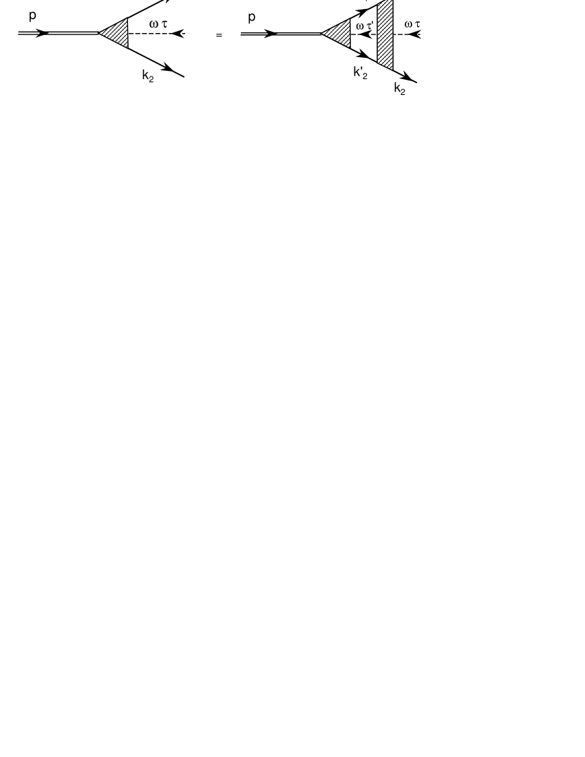
Figure 1: Equation for the two-body wave function.

The kernel of eq. (7) depends on the vector variable $\vec{n}$ and on the bound state mass $M^{2}$. This dependence is associated with the retardation of the interaction.

In the non-relativistic limit the light front wave function turns into the ordinary equal-time wave function. This limit can be formally obtained at $c\to\infty$. Then the light-front plane $t+z/c=0$ turns into the plane $t=0$. Therefore the equation (7) turns into the Schrödinger equation in momentum space, the kernel $V$ being the Fourier-transform of non-relativistic potential and the wave function no longer depends on $\vec{n}$.

4 Simple example

For a given Lagrangian, the amplitudes are calculated by rules of special graph technique, developed in [10] and adjusted to the light-front dynamics in [5]. The diagrams correspond to the time-ordered graphs. The amplitudes on energy-shell coincide with usual Feynman amplitudes on-mass shell. Off the energy and mass shells, these amplitudes differ from each other.

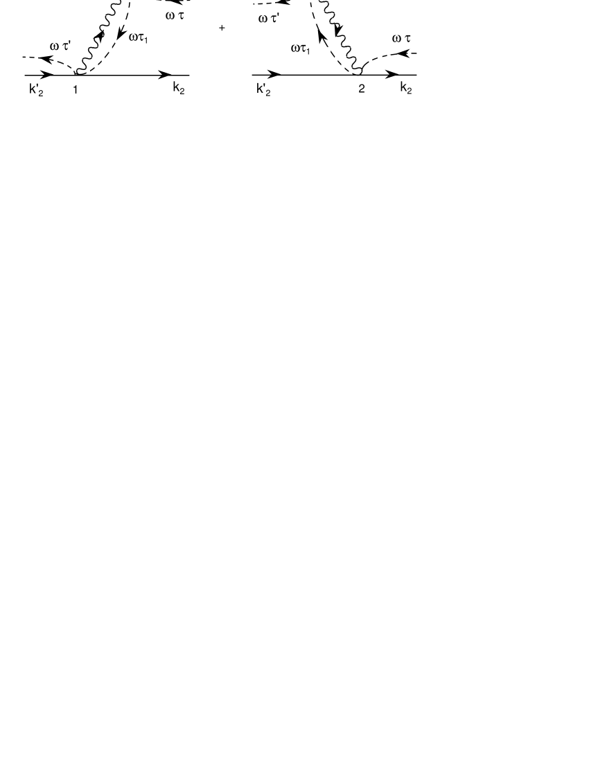
Figure 2: Exchange by a particle in $t$-channel.

Consider exchange in the $t$ channel by a scalar particle of mass $\mu$ between two scalar particles. The amplitude is given by two time-ordered diagrams shown in fig. 2. They determine, in the ladder approximation, the kernel of the equation (7). The external spurion lines indicate that the amplitude is off-energy shell.

According to the light-front graph technique, the amplitude has the form:

$${\cal K}=\frac{g^{2}\theta\left(\omega\makebox[2.27626pt]{$\cdot$}(k_{1}-k^{\prime}_{1})\right)}{\mu^{2}-(k_{1}-k^{\prime}_{1})^{2}+2\tau\omega\makebox[2.27626pt]{$\cdot$}(k_{1}-k^{\prime}_{1})-i\epsilon}+\frac{g^{2}\theta\left(\omega\makebox[2.27626pt]{$\cdot$}(k^{\prime}_{1}-k_{1})\right)}{\mu^{2}-(k^{\prime}_{1}-k_{1})^{2}+2\tau^{\prime}\omega\makebox[2.27626pt]{$\cdot$}(k^{\prime}_{1}-k_{1})-i\epsilon}.$$ (8)

The two items in (8) correspond to the two diagrams of fig. 2. They cannot be non-zero simultaneously. The off-energy shell terms, depending on $\omega$, appear automatically and they are explicitly given in (8). On the energy shell, i.e. for both $\tau=\tau^{\prime}=0$, the expression for the kernel becomes identical to the Feynman amplitude:

$${\cal K}(\tau=\tau^{\prime}=0)=\frac{g^{2}}{\mu^{2}-(k_{1}-k^{\prime}_{1})^{2}-i\epsilon}\ .$$ (9)

In the case of $\mu=0$ we obtain the Wick-Cutkosky model [11], but treated in the framework of CLFD [12]. Going over from the kernel ${\cal K}$ to $V=-{\cal K}/(4m^{2})$, introducing the constant $\alpha=g^{2}/(16\pi m^{2})$, and expressing (8) by means of the initial and final relative momenta $\vec{k},\vec{k}^{\prime}$, we obtain [12]:

$$V=-\frac{4\pi\alpha}{\displaystyle{(\vec{k}\,^{\prime}-\vec{k}\,)^{2}-(\vec{n}\makebox[2.27626pt]{$\cdot$}\vec{k}\,^{\prime})(\vec{n}\makebox[2.27626pt]{$\cdot$}\vec{k})\frac{(\varepsilon_{k^{\prime}}-\varepsilon_{k})^{2}}{\varepsilon_{k^{\prime}}\varepsilon_{k}}+(\varepsilon_{k^{\prime}}^{2}+\varepsilon_{k}^{2}-\frac{1}{2}M^{2})\left|\frac{\vec{n}\makebox[2.27626pt]{$\cdot$}\vec{k}\,^{\prime}}{\varepsilon_{k^{\prime}}}-\frac{\vec{n}\makebox[2.27626pt]{$\cdot$}\vec{k}}{\varepsilon_{k}}\right|}}.$$ (10)

The dependence on the light-front orientation manifests itself in (10) through the vector parameter $\vec{n}$.

The solution of the equation (7) with the kernel (10), in the limit of small binding energy, has the form:

$$\psi(\vec{k},\vec{n})=\frac{8\sqrt{\pi m}\kappa^{5/2}}{(\vec{k}\,^{2}+\kappa^{2})^{2}\left(\displaystyle{1+\frac{|\vec{n}\makebox[2.27626pt]{$\cdot$}\vec{k}|}{\varepsilon_{k}}}\right)}\ .$$ (11)

In non-relativistic limit $k,k^{\prime}\ll m$ the kernel (10) turn into the Coulombien one: $V\approx-4\pi\alpha/(\vec{k}\,^{\prime}-\vec{k}\,)^{2}$ (that in the coordinate space corresponds to $V(r)=-\alpha/r$). The $\vec{n}$-dependent factor in the wave function (11) disappears and the latter turns into the Coulombien wave function too.

We emphasize that the dependence of the wave function (11) on $\vec{n}$ does not mean any violation of the rotational invariance, since this function is a scalar, as should be for the zero angular momentum. However, for non-zero angular momentum, because of Fock space truncation, one can find dependence of energy on the projection of the angular momentum on the $\vec{n}$-direction. This fact indeed means a violation of rotational invariance. A solution of this problem is given in [13].

The solutions of equation (7) with the kernel (10) for $0\leq\mu\leq m$ were studied in [14]. It was found that for the exchange mass $\mu$ comparable with the constituent mass $m$ the relativistic effects in the binding energy are very important even for vanishingly small (”nonrelativistic”) binding energy.

5 Relation with the Bethe-Salpeter function

It is instructive to compare the solution (11) with one found using the Bethe-Salpeter function [15]. The latter is defined as (see for review [16]):

$$\Phi(x_{1},x_{2},p)=\langle 0\left|T(\varphi(x_{1})\varphi(x_{2}))\right|p\rangle.$$ (12)

Here $\varphi(x)$ denotes the field operator in Heisenberg representation. The function (12) depends on two four-vectors $x_{1},x_{2}$, they include two times $t_{1},t_{2}$. Though the Bethe-Salpeter function satisfies the normalization condition, allowing to find the normalization coefficient, it has no any probabilistic interpretation.

In the momentum space the Bethe-Salpeter function looks as: $\Phi=\Phi(q_{1},q_{2},p)$ and is defined through the Fourier transform:

$$\Phi(x_{1},x_{2},p) = (2\pi)^{-3/2}\exp\left[-ip\makebox[2.27626pt]{$\cdot$}(x_{1}+x_{2})/2\right]\tilde{\Phi}(x,p)\ ,\quad x=x_{1}-x_{2}\ ,$$

$$\Phi(q_{1},q_{2},p) = \Phi(q,p)=\int\tilde{\Phi}(x,p)\exp(iq\makebox[2.27626pt]{$\cdot$}x)d^{4}x\ ,$$ (13)

where $q=(q_{1}-q_{2})/2$, $p=q_{1}+q_{2}$, $q_{1}$ and $q_{2}$ are off-mass shell four-vectors: $q_{1}^{2}\neq m^{2}$, $q_{2}^{2}\neq m^{2}$.

In LFD the Heisenberg operators coincide with the Schrödinger ones on the light-front plane (like in the ordinary formulation of field theory the Heisenberg and Schrödinger operators are identical for $t=0$). Therefore, projecting the Bethe-Salpeter function on the light-front, we can relate it to the light-front wave function. In the momentum space this relation reads [7]:

$$\psi(k_{1},k_{2},p,\omega\tau)=\frac{(\omega\makebox[2.27626pt]{$\cdot$}k_{1})(\omega\makebox[2.27626pt]{$\cdot$}k_{2})}{\pi(\omega\makebox[2.27626pt]{$\cdot$}p)}\int_{-\infty}^{+\infty}\Phi(q_{1}=k_{1}-\omega\tau/2+\omega\beta,q_{2}=k_{2}-\omega\tau/2-\omega\beta,p)d\beta$$ (14)

where $\Phi(q_{1},q_{2})$ is the Bethe-Salpeter function (5). The argument $p$ in (14) is related to the on-shell momenta $k_{1},k_{2}$ as $p=k_{1}+k_{2}-\omega\tau$, that follows from the off-mass shell relation $p=q_{1}+q_{2}$.

The equation (14) makes the link between the Bethe-Salpeter function $\Phi$ and the light-front wave function $\psi$. It should be noticed however that the wave function (14) is not necessarily an exact solution of eq. (7), since, as a rule, different approximations are made for the Bethe-Salpeter kernel and for the light-front one. In the ladder approximation, for example, the second iteration of the Bethe-Salpeter amplitude contains the box diagram, including the time-ordered diagram with two exchanged particles in the intermediate state. This contribution is absent in the light-front ladder kernel and in its higer order iterations.

We can check now that in the Wick-Cutkosky model the relation (14) reproduces the wave function (11). In this model, the exact expression for the Bethe-Salpeter function has the form [11, 16]:

$$\Phi(q,p)=-ic\left[\left(m^{2}-\frac{1}{2}M^{2}-q^{2}\right)\left(m^{2}-(\frac{1}{2}p+q)^{2}-i0\right)\left(m^{2}-(\frac{1}{2}p-q)^{2}-i0\right)\right]^{-1},$$ (15)

where $c=2^{5}\sqrt{\pi m\kappa^{5}}$ with $\kappa=\sqrt{m|\epsilon_{b}|}=m\alpha/2$. Substituting (15) in (14), we indeed reproduce the expression (11) for the light-front wave function.

The e.m. form factors calculated through the light-front wave function and through the Bethe-Salpeter one were compared in [8]. They coincide with each other with high accuracy. This means that when both approaches take into account the same relativistic dynamics, they give close results.

However, an important difference between them is in the following. Bethe-Salpeter function (12) is a formally defined object. Whereas, the light-front wave function, being the coefficient in the decomposition (1), according to general principles of quantum theory, is the probability amplitude. It is the same object as nonrelativistic wave function and it has the same physical meaning. Comparing light-front wave function of a relativistic system with its non-relativistic counterpart, we describe the relativistic effects in a language of physical phenomena. This important point is an advantage of LFD. Smooth matching of non-relativistic and relativistic wave functions is also very convenient in practical calculations.

6 Deuteron wave function and form factors

The deuteron wave function is determined by six invariant functions, depending on two scalar variables. This number is the dimension of the matrix depending on the spin projections of the deuteron and two nucleons, divided by the factor 2 due to the parity conservation: $N=3\times 2\times 2/2=6$. This wave function reads:

$$\vec{\psi}(\vec{k},\vec{n}) = f_{1}\frac{1}{\sqrt{2}}\vec{\sigma}+f_{2}\frac{1}{2}\left(\frac{3\vec{k}(\vec{k}\makebox[2.27626pt]{$\cdot$}\vec{\sigma})}{\vec{k}^{2}}-\vec{\sigma}\right)+f_{3}\frac{1}{2}\left(3\vec{n}(\vec{n}\makebox[2.27626pt]{$\cdot$}\vec{\sigma})-\vec{\sigma}\right)$$

$$+ f_{4}\frac{1}{2k}\left(3\vec{k}(\vec{n}\makebox[2.27626pt]{$\cdot$}\vec{\sigma})+3\vec{n}(\vec{k}\makebox[2.27626pt]{$\cdot$}\vec{\sigma})-2(\vec{k}\makebox[2.27626pt]{$\cdot$}\vec{n})\vec{\sigma}\right)+f_{5}\sqrt{\frac{3}{2}}\frac{i}{k}\left[\vec{k}\times\vec{n}\right]+f_{6}\frac{\sqrt{3}}{2k}\left[[\vec{k}\times\vec{n}]\times\vec{\sigma}\right].$$

In the relativistic one boson exchange model it was calculated in [17]. The results are displayed in fig. 3.

Figure 3: Deuteron relativistic components $f_{1}-f_{6}$ as a function of $k$, at $\vec{n}\vec{k}/k=0.6$.

One can see that the function $f_{5}$, of relativistic origin, is very important: it dominates at $k>500$ MeV/c. In [18] it was shown that this component dominates since it automatically takes into account the isovector exchange currents (so called pair terms). They should not be added separately. In nonrelativistic limit the functions $f_{3-6}$ become negligible and only two first functions $f_{1,2}$, corresponding to usual S- and D-waves, survive.

This wave function was used in [1, 7] to calculate the deuteron electromagnetic form factors. No any parameters were fitted. It turned out that the calculated polarization observable $t_{20}$, fig. 5, as well as the charge and quadrupole form factors, fig. 5, coincide with rather precise experimental data obtained recently at CEBAF/TJNAF [19].

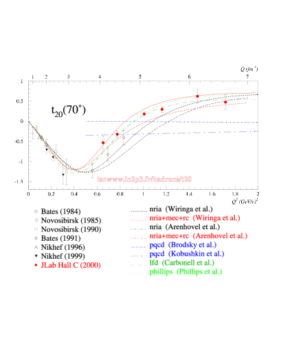
Figure 4: Polarization observable $t_{20}$ in $ed$ scattering, taken from [20].

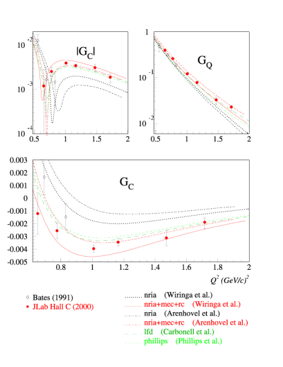
Figure 5: Charge and quadrupole deuteron form factors, taken from [20].

7 Three-boson bound states with zero-range interaction

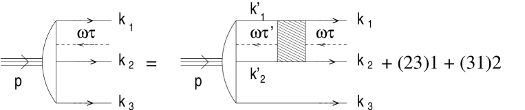
Figure 6: Three-body equation for the vertex function $\Gamma$.

The most recent application of CLFD is the relativistic system of three-bosons with zero range interaction. We will describe it in more detail.

Zero-range two-body interaction provides an important limiting case which qualitatively reflects characteristic properties of nuclear and atomic few-body systems. In the nonrelativistic three-body system it generates the Thomas collapse [21]. The latter means that the three-body binding energy tends to $-\infty$, when the interaction radius tends to zero.

When the binding energy or the exchanged particle mass is not negligible in comparison to the constituent masses, the nonrelativistic treatment becomes invalid and must be replaced by a relativistic one. Two-body calculations show that in the scalar case, relativistic effects are repulsive (see e.g. [14]). Relativistic three-body calculations with zero-range interaction have been performed in a minimal relativistic model [22] and in the framework of the Light-Front Dynamics [23]. In these works it was concluded that, due to relativistic repulsion, the three-body binding energy remains finite and the Thomas collapse is consequently avoided. However, in the papers [22, 23] a cutoff has been introduced implicitly. Being interested in studing the zero-range interaction as an important limiting case, we eliminate this cutoff.

The three-body equation is represented graphically in figure 6. It concerns the vertex function $\Gamma$, related to the wave function $\psi$ in the standard way:

$$\psi(k_{1},k_{2},k_{3},p,\omega\tau)=\frac{\Gamma(k_{1},k_{2},k_{3},p,\omega\tau)}{{\cal M}^{2}-M^{2}_{3}},\quad{\cal M}^{2}=(k_{1}+k_{2}+k_{3})^{2}=(p+\omega\tau)^{2}.$$

Like for the two-body system, all four-momenta are on the corresponding mass shells: $k_{i}^{2}=m^{2},p^{2}=M_{3}^{2},(\omega\tau)^{2}=0$ and satisfy the conservation law $k_{1}+k_{2}+k_{3}=p+\omega\tau$ involving $\omega\tau$.

Applying to figure 6 the covariant light-front graph techniques [7], we find:

$$\Gamma(k_{1},k_{2},k_{3},p,\omega\tau)=\frac{\lambda}{(2\pi)^{3}}\int\Gamma(k^{\prime}_{1},k^{\prime}_{2},k_{3},p,\omega\tau^{\prime})$$

$$\times\delta^{(4)}(k^{\prime}_{1}+k^{\prime}_{2}-\omega\tau^{\prime}-k_{1}-k_{2}+\omega\tau)\frac{d\tau^{\prime}}{\tau^{\prime}}\,\frac{d^{3}k^{\prime}_{1}}{2\varepsilon_{k^{\prime}_{1}}}\,\frac{d^{3}k^{\prime}_{2}}{2\varepsilon_{k^{\prime}_{2}}}\;+\;(23)1+(31)2,$$ (17)

where $\varepsilon_{k}=\sqrt{m^{2}+\vec{k}^{2}}$. For zero-range forces, the interaction kernel is replaced in (7) by a constant $\lambda$. The contribution of interacting pair 12 is explicitly written while the contributions of the remaining pairs are denoted by $(23)1+(31)2$.

The Faddeev amplitudes $\Gamma_{ij}$ are introduced in the standard way:

$$\Gamma(1,2,3)=\Gamma_{12}(1,2,3)+\Gamma_{23}(1,2,3)+\Gamma_{31}(1,2,3),$$

and equation (7) is equivalent to a system of three coupled equations. With the symmetry relations $\Gamma_{23}(1,2,3)=\Gamma_{12}(2,3,1)$ and $\Gamma_{31}(1,2,3)=\Gamma_{12}(3,1,2)$, the system is reduced to a single equation for one of the amplitudes, say $\Gamma_{12}$.

We use the tree-body version of the variables defined in eq. (4). In general, $\Gamma_{12}$ depends on all variables ($\vec{R}_{i\perp},x_{i}$), constrained by the relations $\vec{R}_{1\perp}+\vec{R}_{2\perp}+\vec{R}_{3\perp}=0$, $x_{1}+x_{2}+x_{3}=1$, but for contact kernel it depends only on $(\vec{R}_{3\perp},x_{3})$ [23].

The value of $\lambda$ is found analytically by solving the two-body problem with the same zero-range interaction under the condition that the two-body bound state mass has a fixed value $M_{2}$. In this way, the constant $\lambda$ disappears from the kernel, but the two-body scattering amplitudes appears, as in any Faddeev equations. For the zero-range interaction, this amplitude does not depend on the relative momentum, but depends on the off-energy shell variables. Therefore it is extracted from the integral. Finally, the equation for the Faddeev amplitude reads:

$$\Gamma_{12}(R_{\perp},x)=F(M_{12})\frac{\displaystyle{1}}{\displaystyle{(2\pi)^{3}}}\displaystyle{\int_{0}^{1}}\displaystyle{dx^{\prime}}\displaystyle{\int_{0}^{\infty}}\frac{\Gamma_{12}\left(R^{\prime}_{\perp},x^{\prime}(1-x)\right)\;d^{2}R^{\prime}_{\perp}}{\displaystyle{(\vec{R^{\prime}}_{\perp}-x^{\prime}\vec{R}_{\perp})^{2}+m^{2}-x^{\prime}(1-x^{\prime})M_{12}^{2}}},$$ (18)

where $F(M_{12})$ is the two-body off-shell scattering amplitude:

$$\frac{F(M_{12})}{8\pi^{2}}=\left\{\begin{array}[]{l}\left[\frac{\displaystyle{1}}{\displaystyle{2y^{\prime}_{M_{12}}}}\log\frac{\displaystyle{1+y^{\prime}_{M_{12}}}}{\displaystyle{1-y^{\prime}_{M_{12}}}}-\frac{\displaystyle{\arctan y_{M_{2}}}}{\displaystyle{y_{M_{2}}}}\right]^{-1},\quad M_{12}^{2}<0,\quad y^{\prime}_{M_{12}}=\frac{\sqrt{-M_{12}^{2}}}{\sqrt{4m^{2}-M_{12}^{2}}}\\ \\ \left[\frac{\displaystyle{\arctan y_{M_{12}}}}{\displaystyle{y_{M_{12}}}}-\frac{\displaystyle{\arctan y_{M_{2}}}}{\displaystyle{y_{M_{2}}}}\right]^{-1},\quad 0\leq M_{12}^{2}<4m^{2},\quad y_{M_{12}}=\frac{M_{12}}{\sqrt{4m^{2}-M_{12}^{2}}}\end{array}\right.$$

and similarly for $y_{M_{2}}=\frac{M_{2}}{\sqrt{4m^{2}-M_{2}^{2}}}$. The variable $M^{2}_{12}=(k^{\prime}_{1}+k^{\prime}_{2}-\omega\tau^{\prime})^{2}=(p-k_{3})^{2}$ is the off-shell mass of the two-body subsystem. It is expressed through $M_{3}^{2},R_{\perp}^{2},x$ as

$$M^{2}_{12}=(1-x)M_{3}^{2}-\frac{R_{\perp}^{2}+(1-x)m^{2}}{x}.$$ (19)

The three-body mass $M_{3}$ enters in the equation (18) through variable $M_{12}^{2}$.

By replacing $x^{\prime}(1-x)\to x^{\prime}$, equation (18) can be transformed to

$$\Gamma_{12}(R_{\perp},x)=F(M_{12})\frac{\displaystyle{1}}{\displaystyle{(2\pi)^{3}}}\displaystyle{\int_{0}^{1-x}}\frac{\displaystyle{dx^{\prime}}}{\displaystyle{x^{\prime}(1-x-x^{\prime})}}\;\displaystyle{\int_{0}^{\infty}}\frac{\displaystyle{d^{2}R^{\prime}_{\perp}}}{\displaystyle{{{\cal M}^{\prime}}^{2}-M_{3}^{2}}}\;\Gamma_{12}\left(R^{\prime}_{\perp},x^{\prime}\right),$$ (20)

where

$${{\cal M}^{\prime}}^{2}=\frac{\vec{R^{\prime}}^{2}_{\perp}+m^{2}}{x^{\prime}}+\frac{\vec{R}^{2}_{\perp}+m^{2}}{x}+\frac{(\vec{R^{\prime}}_{\perp}+\vec{R}_{\perp})^{2}+m^{2}}{1-x-x^{\prime}}.$$

This equation is the same than equation (11) from [23] except for the integration limits of ($\vec{R^{\prime}}_{\perp},x^{\prime}$) variables. In [23] the integration limits follow from the condition $M_{12}^{2}>0$. They read

$$\int_{m^{2}\over M_{3}^{2}}^{1-x}\left[\ldots\right]dx^{\prime}\int_{0}^{k^{max}_{\perp}}\left[\ldots\right]d^{2}R^{\prime}_{\perp}$$ (21)

with $k^{max}_{\perp}=\sqrt{(1-x^{\prime})(M_{3}^{2}x^{\prime}-m^{2})}$ and introduce a lower bound on the three-body mass $M_{3}>\sqrt{2}m$. The same condition, though in a different relativistic approach, was used in [22]. The integration limits in (21) restrict the arguments of $\Gamma_{12}$ to the domain

$${m^{2}\over M_{3}^{2}}\leq x\leq 1-{m^{2}\over M_{3}^{2}},\quad 0\leq R_{\perp}\leq k_{\perp}^{max}$$

and can be considered as a method of regularization. In this case, one no longer deals with the zero-range forces.

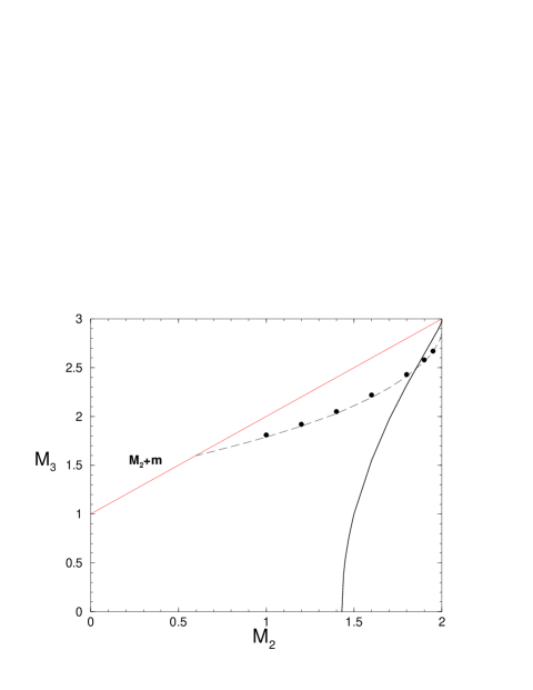
(a)

(b)

Figure 7: (a) Three-body bound state mass $M_{3}$ versus the two-body one $M_{2}$ (solid line). Results obtained with integration limits (21) are in dash line. Dots values are taken from [24]. (b) Zoom of the zero two-body binding region ($M_{2}\to 2m,B_{2}\to 0$) displaying solid line only.

The results of solving equation (18) are presented in what follows. Calculations were carried out with constituent mass $m=1$ and correspond to the ground state. We represent in fig. 7a the three-body bound state mass $M_{3}$ as a function of the two-body one $M_{2}$ (solid line) together with the dissociation limit $M_{3}=M_{2}+m$. The zero two-body binding limit $B_{2}=2m-M_{2}\to 0$ is magnified in fig. 7b. In this limit the three-boson system has a binding energy $B_{3}\approx 0.012$.

When $M_{2}$ decreases, the three-body mass $M_{3}$ decreases very quickly and vanishes at the two-body mass value $M_{2}=M_{c}\approx 1.43$. Whereas the meaning of collapse as used in the Thomas paper implies unbounded nonrelativistic binding energies and cannot be used here, the zero bound state mass $M_{3}=0$ constitutes its relativistic counterpart. Indeed, for two-body masses below the critical value $M_{c}$, the three-body system no longer exists.

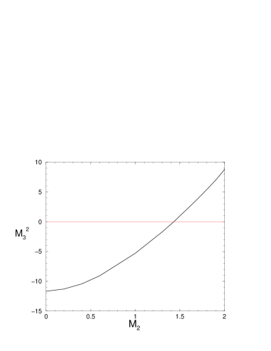
Figure 8: Three-body bound state mass squared $M_{3}^{2}$ versus $M_{2}$.

The results corresponding to integration limits (21) are included in fig. 7a (dash line) for comparison. Values given in [23] were not fully converged [25]. They have been corrected in [24] and are indicated by dots. In both cases the repulsive relativistic effects produce a natural cutoff in equation (18), leading to a finite spectrum and – in the Thomas sense – an absence of collapse, like it was already found in [22]. However, except in the zero binding limit, solid and dash curves strongly differ from each other.

We would like to remark that for $M_{2}\leq M_{c}$, equation (18) posses square integrable solutions with negative values of $M_{3}^{2}$. They have no physical meaning but $M_{3}^{2}$ remains finite in all the two-body mass range $M_{2}\in[0,2]$. The results of $M_{3}^{2}$ are given in figure 8. When $M_{2}\to 0$, $M_{3}^{2}$ tends to $\approx-11.6$.

From the above results we conclude that the three-body bound state exists for two-body mass values in the range $M_{c}\approx 1.43\,m\leq M_{2}\leq 2\,m$. At the zero two-body binding limit, the three-body binding energy is $B_{3}\approx 0.012\,m$. The Thomas collapse is avoided in the sense that three-body mass $M_{3}$ is finite, in agreement with [22, 23]. However, another kind of catastrophe happens. Removing infinite binding energies, the relativistic dynamics generates zero three-body mass $M_{3}$ at a critical value $M_{2}=M_{c}$. For stronger interaction, i.e. when $0\leq M_{2}<M_{c}$, there are no physical solutions with real value of $M_{3}$. In this domain, $M_{3}^{2}$ becomes negative and the three-boson system cannot be described by zero range forces, as it happens in nonrelativistic dynamics. This fact can be interpreted as a relativistic collapse.

8 Conclusion

We have seen that the explicitly covariant light-front dynamics provides a very satisfactory framework, both from a theoretical and practical points of view, for describing relativistic nucleons in deuteron and other nuclei. The predicted deuteron electromagnetic form factors, calculated without any fitting parameters, are in good agreement with experimental data.

This approach is also successfully when applied to many other problems and a consequent effort covering several directions of research is actually being performed. Here is a list of current applications.

• Deuteron wave function [17] and form factors [1, 7].

• Nucleon momentum distributions in nuclei [2].

• Leptonic decay of heavy quarkonia [26].

• Fock-space expansion [27].

• Nucleon wave function [28] and neutron charge radius [29] in quark model.

• Two-fermion relativistic bound states [30, 31].

• Perturbative [32] and non perturbative [33] renormalization.

• Three-boson relativistic bound states [34].

We conclude that the explicitly covariant light-front dynamics is a rather efficient approach to relativistic few-body systems and to field theory.

This work is supported by the French-Russian PICS and RFBR grants Nos. 1172 and 01-02-22002.

References

- [1] J. Carbonell, V.A. Karmanov, Eur. Phys. J. A6 (1999) 9.
- [2] A.N. Antonov, M. Gaidarov, M.V. Ivanov, D.N. Kadrev, G.Z. Krumova , P.E. Hodgson and H.V. von Geramb, Phys. Rev. C65 (2002) 024306.
- [3] P.A.M. Dirac, Rev. Mod. Rhys. 21 (1949) 392.
- [4] S. Weinberg, Phys. Rev. 150 (1966) 1313.
- [5] V.A. Karmanov, ZhETF, 71 (1976) 399 [transl.: JETP, 44 (1976) 210].
- [6] V.A. Karmanov, Fiz. Elem. Chastits At. Yadra, 19 (1988) 525 [Sov. J. Part. Nucl. 19 (1988) 228].
- [7] J. Carbonell, B. Desplanques, V.A. Karmanov and J.-F. Mathiot, Phys. Reports, 300 (1998) 215.
- [8] V.A. Karmanov and A.V. Smirnov, Nucl. Phys. A546 (1992) 691; A575 (1994) 520.
- [9] V.A. Karmanov and J.-F. Mathiot, Nucl. Phys. A602 (1996) 388.
- [10] V.G. Kadyshevsky, ZhETF, 46 (1964) 654, 872 [JETP, 19 (1964) 443, 597]; Nucl. Phys. B6 (1968) 125.
-
[11]
G.C. Wick Phys. Rev. 96 (1954) 1124;
R.E. Cutkosky, Phys. Rev. 96 (1954) 1135. - [12] V.A. Karmanov, Nucl. Phys. B166 (1980) 378.
- [13] V.A. Karmanov, M. Mangin-Brinet, J. Carbonell, Nucl.Phys. A684 (2001) 366.
- [14] M. Mangin-Brinet, J. Carbonell, Phys. Lett. B474, (2000) 237
- [15] E.E. Salpeter and H.A. Bethe, Phys. Rev. 84 (1951) 1232.
- [16] N. Nakanishi, Prog. Theor. Phys. Suppl. 43 (1969) 1; 95 (1988) 1.
- [17] J. Carbonell and V.A. Karmanov, Nucl. Phys. A581 (1995) 625.
- [18] B. Desplanques, V.A. Karmanov and J.-F. Mathiot, Nucl. Phys. A589 (1995) 697.
- [19] D. Abbott et al., Phys.Rev.Lett. 84 (2000) 5053.
- [20] http://isnwww.in2p3.fr/hadrons/hadrons.html
- [21] L.H. Thomas, Phys. Rev. 47 (1935) 903.
- [22] J.V. Lindesay and H.P. Noyes, Preprint SLAC-PUB-2932, 1986.
- [23] T. Frederico, Phys. Lett. B282 (1992) 409.
- [24] W.R.B. de Araujo, J.P.B.C. de Melo, T. Frederico, Phys. Rev. C52 (1995) 2733.
- [25] T. Frederico, private communication.
- [26] F. Bissey, J-J. Dugne, J-F. Mathiot, Eur. Phys. J. C24 (2002) 101.
- [27] N.C.J. Schoonderwoerd, B.L.G. Bakker and V.A. Karmanov, Phys. Rev. C58 (1998) 3093.
- [28] V.A. Karmanov, Nucl. Phys. A 644 (1998) 165.
- [29] V.A. Karmanov, Nucl.Phys. A699 (2002) 148.
- [30] M. Mangin-Brinet, J. Carbonell, V.A. Karmanov, Phys. Rev. D64 (2001) 027701; D64 (2001) 125005.
- [31] J.Carbonell, M. Mangin-Brinet, V.A. Karmanov, Nucl. Phys. Proc. Suppl. 108 (2002) 256-258; The XIVth International School on Nuclear Physics, Varna, Bulgaria, Sept 25-30, 2001; nucl-th/0202042.
- [32] J.-J. Dugne, V.A. Karmanov, J.-F. Mathiot, Eur. Phys. J. C22 (2001) 105.
- [33] D. Bernard, Th. Cousin, V.A. Karmanov, J.-F. Mathiot, Phys. Rev. D65 (2002) 025016.
- [34] J. Carbonell, V.A. Karmanov, nucl-th/0207073; submitted for publication.