Vector meson production and nucleon resonance analysis in a coupled-channel approach for energies $m_{N}<\sqrt{s}<2$ GeV
I: pion-induced results and hadronic parameters

Abstract

We present a nucleon resonance analysis by simultaneously considering all pion- and photon-induced experimental data on the final states $\gamma N$, $\pi N$, $2\pi N$, $\eta N$, $K\Lambda$, $K\Sigma$, and $\omega N$ for energies from the nucleon mass up to $\sqrt{s}=2$ GeV. In this analysis we find strong evidence for the resonances $P_{31}(1750)$, $P_{13}(1900)$, $P_{33}(1920)$, and $D_{13}(1950)$. The $\omega N$ production mechanism is dominated by large $P_{11}(1710)$ and $P_{13}(1900)$ contributions. In this first part, we present the results of the pion-induced reactions and the extracted resonance and background properties with emphasis on the difference between global and purely hadronic fits.

I Introduction

The reliable extraction of nucleon resonance properties from experiments where the nucleon is excited via either hadronic or electromagnetic probes is one of the major issues of hadron physics. The goal is to be finally able to compare the extracted masses and partial-decay widths to predictions from lattice QCD (e.g., Ref. flee ) and/or quark models (e.g., Refs. capstick ; riska ).

Basically all information about nucleon resonances identified so far from experiment pdg stems from analyses of pion-induced $\pi N$ and $2\pi N$ production manley92 ; arndt95 ; vrana , and also from pion photoproduction arndt96 ; arndt02 . However, it is well known that, for example, in the case of the $S_{11}(1535)$ the consideration of the $\eta N$ final state is inevitable to extract its properties reliably, and similar effects can be expected for higher lying resonances and different thresholds. Only in the analysis of Vrana et al. vrana the model space has been extended to also include information on $\pi N\rightarrow\eta N$ in the comparison with experimental data. On the other side, quark models predict a much richer resonance spectrum than has been found in $\pi N$ and $2\pi N$ production so far, giving rise to speculations that many of these resonance states only become visible in other reaction channels. This is the basis for a wealth of analyses concentrating on identifying these “missing” or “hidden” resonances in the production of other final states as $\eta N$, $K\Lambda$, $K\Sigma$, or $\omega N$. For a consistent identification of those resonances and their properties, the consideration of unitarity effects are inevitable and as many final states as possible have to be taken into account simultaneously. With this aim in mind we developed in Refs. feusti98 ; feusti99 a unitary coupled-channel effective Lagrangian model (Giessen model) that incorporated the final states $\gamma N$, $\pi N$, $2\pi N$, $\eta N$, and $K\Lambda$ and was used for a simultaneous analysis of all available experimental data on photon- and pion-induced reactions on the nucleon. In later studies the model was used to also analyze kaon-induced reactions matze and for a first investigation on $\pi N\rightarrow K\Sigma$ agung . The premise is to use the same Lagrangians for the pion- and photon-induced reactions allowing for a consistent analysis, thereby generating the background dynamically from $u$- and $t$-channel contributions without new parameters.

In an extension of the model to higher center-of-mass energies, i.e., up to c.m. energies of $\sqrt{s}=2$ GeV for the investigation of higher and hidden or missing nucleon resonances, the consideration of the $\omega N$ state in a unitary model is mandatory. Furthermore, $\omega$ production on the nucleon represents a possibility to project out $I=\frac{1}{2}$ resonances in the reaction mechanism. The inclusion of $K\Sigma$ gives additional information on resonance properties, since especially in the pure $I=\frac{3}{2}$ reaction $\pi^{+}p\rightarrow K^{+}\Sigma^{+}$ many data have been taken in the $1960$s and $1970$s. It is also known nobby that the inclusion of the $K\Sigma$ final state can have an important influence on the description of $K\Lambda$ observables. Hence we have extended the model of Refs. feusti98 ; feusti99 to also include $\omega N$ and $K\Sigma$.

For the newly incorporated channels $\omega N$ and $K\Sigma$, almost all models in the literature are based on single-channel effective Lagrangian calculations, ignoring rescattering effects (often called “$T$-matrix models”) and thereby the influence of the extracted resonance properties on other reaction channels. This problem can only be circumvented if all channels are compared simultaneously to experimental data thereby restricting the freedom severely; this is done in the model underlying the present calculation. To our knowledge, the only other calculation considering the $\omega N$ channel in a coupled-channel approach is the model by Lutz et al. lutz , where pointlike interactions are used. There, the complexity of the vector-meson nucleon states is further simplified by the use of only one specific combination of the $VN$ helicity states (cf. Appendix A). Due to the lack of $J^{P}=\frac{1}{2}^{+}$ and $J^{P}=\frac{3}{2}^{+}$ $(P)$ waves in their model, these authors are only able to compare to production cross sections at energies very close to the corresponding threshold by assuming $S$-wave dominance. The photon coupling is implemented via strict vector meson dominance (VMD), i.e., the photon can only couple to any other particle via its “hadronic” components, the $\rho$ and $\omega$ mesons.

In Ref. gregi we have presented our first results on the analysis of the pion-induced reactions. In this work, we give a comprehensive discussion of the results for the pion-induced reactions, both with and without additionally taking into account the photoproduction data, which allow us to pin down the resonant contributions even more reliably. The results of the photoproduction reactions themselves are presented in the succeeding paper pm2 , called PMII in the following. Hence this analysis differs from all other resonance analyses by its larger channel space. For the investigation of the $\pi N\rightarrow\omega N$ channel, this calculation is different from other models in the following respects: First, a larger energy region is considered, which also means there are more restrictions from experiment, second, the reaction process is influenced by all other channels and vice versa, and third, also a large $\omega$ photoproduction data base is taken into account. This leads to strong constraints in the choice of $\omega N$ contributions, and it is therefore possible to extract these more reliably.

We start in Sec. II with a review of the model of Ref. feusti98 ; feusti99 ; gregi with special emphasis on the extensions. In Sec. III the performed calculations are described and in Sec. IV these calculations are compared to the available experimental data. We conclude with a summary. In the appendices, we give a self-contained summary of the full formalism underlying the present model; more details can be found in Ref. gregiphd . The formalism and the results for the photon-induced reactions are given in PMII pm2 .

II Giessen Model

The scattering equation that needs to be solved is the Bethe-Salpeter (BS) equation for the scattering amplitude:

$$M(p^{\prime},p;\sqrt{s})=V(p^{\prime},p;\sqrt{s})+\int\frac{\mathrm{d}^{4}q}{(2\pi)^{4}}V(p^{\prime},q;\sqrt{s})G_{BS}(q;\sqrt{s})M(q,p;\sqrt{s})$$ (1)

in the notation given in Appendix A. Here, $p$ ($k$) and $p^{\prime}$ ($k^{\prime}$) are the incoming and outgoing baryon (meson) four-momenta. After splitting up the two-particle BS propagator $G_{BS}$ into its real and imaginary parts, one can introduce the $K$ matrix via (in a schematical notation) $K=V+\int V\mathrm{Re}G_{BS}M$. Then $M$ is given by $M=K+i\int M\mathrm{Im}G_{BS}K$. Since the imaginary part of $G_{BS}$ just contains its on-shell part

$$\mbox{i}\mathrm{Im}(G_{BS}(q))=-\mbox{i}\pi^{2}\frac{m_{B_{q}}\sum_{\lambda_{B_{q}}}u(p_{q},\lambda_{B_{q}})\bar{u}(p_{q},\lambda_{B_{q}})}{E_{B_{q}}E_{M_{q}}}\delta(k_{q}^{0}-E_{M_{q}})\delta(p_{q}^{0}-E_{B_{q}})\;,$$ (2)

the BS equation simplifies to

$${\mathcal{T}}^{fi}_{\lambda^{\prime}\lambda}={\mathcal{K}}^{fi}_{\lambda^{\prime}\lambda}+\mbox{i}\int\mathrm{d}\Omega_{a}\sum_{a}\sum_{\lambda_{a}}{\mathcal{T}}^{fa}_{\lambda^{\prime}\lambda_{a}}{\mathcal{K}}^{ai}_{\lambda_{a}\lambda}\;,$$ (3)

where we have introduced the ${\mathcal{T}}$ and ${\mathcal{K}}$ amplitudes defined in Appendix A. $a$ represents the intermediate two-particle state. As shown in Appendix B this can be further simplified for parity conserving and rotationally invariant interactions by a partial-wave decomposition in $J$, $P$, and $I$ and one arrives at an algebraic equation relating the decomposed ${\mathcal{T}}^{fi}$and ${\mathcal{K}}^{fi}$:

$${\mathcal{T}}^{IJ\pm}_{fi}=\left[\frac{{\mathcal{K}}^{IJ\pm}}{1-\mbox{i}{\mathcal{K}}^{IJ\pm}}\right]_{fi}\;.$$ (4)

Hence unitarity is fulfilled as long as ${\mathcal{K}}$ is Hermitian.

To date, a full solution of the BS Equation (1) in the meson-baryon sector has only been possible for low-energy $\pi N$ scattering lahiff , i.e., where no other channels are important. Consequently, various approximations to the BS Equation (1) preserving unitarity can be found in the literature. Many of these approximations reduce the four-dimensional BS Equation (1) to a three-dimensional Lippmann-Schwinger equation. However, due to technical feasibility, most of them are restricted to elastic pion-nucleon scattering, while only a few ones also include inelastic channels gross ; krehl . A general problem of the three-dimensional (3D) reduction is the way the reduction is performed. There is no unique method gross ; it can even be shown that the 3D reduction can be achieved in an infinite number of ways, all of which satisfy Lorentz invariance and elastic two-body unitarity yaes . In view of the number of parameters that have to be determined by comparison of our effective Lagrangian calculation with experimental data, we apply the so-called $K$-matrix Born approximation, which is the only feasible method that still satisfies the important condition of unitarity. In the $K$-matrix Born approximation, the real part of $G_{BS}$ is neglected and thus $K$ reduces to $K=V$.

The validity of the effective Lagrangian $K$-matrix method as compared to calculations accounting also for analyticity has first been tested by Pearce and Jennings pearce . By fitting the $\pi N$ elastic phase shifts up to $\approx 1.38$ GeV with various approximations to the intermediate two-particle propagator $G_{BS}$, these authors have found no significant differences in the parameters extracted in the various schemes. It has also been deduced that the contributions of $G_{BS}$ to the principal value part of the scattering equation are of minor importance, since they have been reduced by a very soft cutoff dictated by experimental data. It has been concluded that — in order to fulfill the low-energy theorems — an important feature of the reduced intermediate two-particle propagator is a delta function on the energy transfer. It has also been argued in goudsmit , that for $\pi N$ scattering the main effect of the real part of the intermediate loop integrals is a renormalization of the coupling constants and masses of the involved particles. Therefore in the present $K$-matrix calculation these are taken to be physical values and are either taken from other reliable sources (if available) or to be determined by comparison with experimental data.

It should be mentioned that within the $K$-matrix method the nature of a resonance as a genuine three-quark excitation or dynamic scattering resonance cannot be determined. There are, e.g., hints, that the Roper $P_{11}(1440)$ resonance is a quasibound $\sigma N$ state krehl . In addition, in the chiral models of Refs. nobby and inoue the $S_{11}(1535)$ can be explained as a quasibound meson-baryon ($K\Sigma$ and $\eta N$) state. Moreover, it has been shown in Ref. denschlag by using a generalized separable Lee model, that explicit $S_{11}(1535)$ resonance contributions might not play a large role if the coupled-state system $\pi N\oplus\eta N$ is treated analytically, i.e., the real part of the Bethe-Salpeter propagator $G_{BS}$ is taken into account. Because of the neglect of the real part of $G_{BS}$ in the $K$-matrix approximation, these resonances cannot be generated dynamically as quasibound meson-baryon states, but have to be put into the potential explicitly. We note, however, that a clean distinction between dynamic and quark-state resonances is very difficult, if not impossible. If at all possible, it may require more and other data than analyzed here, in particular also from electroproduction (see, e.g., Ref. burkert ), where information on the spatial extent of the states can be obtained.

II.1 Potential

The interaction potential in the Giessen model is determined by the inclusion of $s$-, $u$-, and $t$-channel contributions generated by means of an effective generic Lagrangian,

$${\mathcal{L}}={\mathcal{L}}_{Born}+{\mathcal{L}}_{t}+{\mathcal{L}}_{Res}\;,$$ (5)

where ${\mathcal{L}}_{Born}+{\mathcal{L}}_{t}$ is given fully in Eq. (35) and the resonance Lagrangians are summarized in Appendices C.2 and C.3. Consequently, the background is dynamically generated by the Born terms (${\mathcal{L}}_{Born}$), the $t$-channel exchanges (${\mathcal{L}}_{t}$), and the $u$-channel contributions of the resonance couplings (${\mathcal{L}}_{Res}$). Since these background terms give contributions to all partial waves simultaneously, the number of free parameters is largely reduced.

II.1.1 Background contributions

In this section, we discuss the ingredients of the Born and $t$-channel Lagrangian ${\mathcal{L}}_{Born}+{\mathcal{L}}_{t}$ of Eq. (5), where the $\pi N$ part underlies special constraints due to chiral symmetry.

Since an effective hadronic interaction Lagrangian should resemble the underlying fundamental theory QCD as closely as possible, the interaction also should be in conformity with chiral symmetry, which is known to be important for low-energy $\pi N$ physics. We choose Weinberg’s nonlinear realization weinberg68 and thus pseudovector pion-nucleon coupling: $\gamma_{5}\gamma_{\mu}\partial^{\mu}\mbox{\boldmath$\pi\!\!$ \unboldmath}\!\cdot\!\mbox{\boldmath$\tau\!\!$ \unboldmath}$ and identify the Weinberg-Tomazawa contact term weinbergtomazawa ; weinberg68 , which automatically accounts for the values of the $\pi N$ scattering lengths, with a $\rho$ meson exchange. Thus the $\rho$ couplings should be fixed by the Kawarabayashi-Suzuki-Riazuddin-Fayyazuddin (KSRF) relation ksrf : $\sqrt{g_{\rho}g_{\rho\pi\pi}}=m_{\rho}/(2f_{\pi})$ with the pion-decay constant $f_{\pi}=93$ MeV, which gives $g_{\rho}\approx 2.84$ using the value $g_{\rho\pi\pi}=6.02$. It should be remarked that this equivalence only holds at threshold, while the energy dependence of the $\rho$ exchange is different from the Weinberg-Tomazawa contact term. Since the aim of the present calculation is the analysis of a wide energy region, we allow for deviations from the KSRF relation by varying the $\rho$ nucleon coupling $g_{\rho}$.

In the nonlinear chiral symmetry realization the $\sigma$ meson is not needed. Nevertheless, a $t$-channel $\sigma$ exchange can be used to model an effective interaction, representing higher-order processes such as the correlated $2\pi$ exchange in the scalar-isoscalar wave, which is not explicitly included in our potential. In order to keep the agreement with chiral symmetry and the soft-pion theorem, the derivative coupling of the sigma to the pion $(\sigma\partial_{\mu}\mbox{\boldmath$\pi\!\!$ \unboldmath}\partial^{\mu}\mbox{\boldmath$\pi\!\!$ \unboldmath})$ should be used. Indeed, in the $\pi N$ sector the background part of ${\mathcal{L}}$ of Eq. (5) respects chiral symmetry and is identical to that used in Refs. pearce ; lahiff ; pascatjon :

$${\mathcal{L}}_{\chi}=-\bar{u}\left[\frac{g_{\pi}}{2m_{N}}\gamma_{5}\gamma_{\mu}(\partial^{\mu}\mbox{\boldmath$\pi\!\!$ \unboldmath})\mbox{\boldmath$\tau\!\!$ \unboldmath}+g_{\sigma}\sigma+g_{\rho}\left(\gamma_{\mu}-\frac{\kappa_{\rho}}{2m_{N}}\sigma_{\mu\nu}\partial^{\nu}_{\rho}\right)\mbox{\boldmath$\rho\!\!$ \unboldmath}^{\mu}\mbox{\boldmath$\tau\!\!$ \unboldmath}\right]u-\frac{g_{\sigma\pi\pi}}{2m_{\pi}}(\partial_{\mu}\mbox{\boldmath$\pi\!\!$ \unboldmath})(\partial^{\mu}\mbox{\boldmath$\pi\!\!$ \unboldmath}^{\prime})\sigma-g_{\rho\pi\pi}\left(\mbox{\boldmath$\pi\!\!$ \unboldmath}\times(\partial_{\mu}\mbox{\boldmath$\pi\!\!$ \unboldmath}^{\prime})\right)\mbox{\boldmath$\rho\!\!$ \unboldmath}^{\mu}\;.$$ (6)

Note that in Refs. feusti98 ; feusti99 the sigma meson had not been included. To investigate the effects of chiral symmetry breaking, we have also performed a calculation using a direct $\sigma\mbox{\boldmath$\pi\!\!$ \unboldmath}\mbox{\boldmath$\pi\!\!$ \unboldmath}$ coupling as in Refs. pascatjon ; goudsmit .

Since the $\sigma$ meson is supposed to model the scalar-isoscalar two-pion correlated exchange, its mass $m_{\sigma}$ is a priori not fixed. In Ref. pearce ; lahiff $m_{\sigma}$ was thus used as a free parameter and fitted to $\pi N\rightarrow\pi N$ data. In our calculation, it turns out that the final quality of the fit is almost independent of the actual value. As long as it is in a reasonable range of $m_{\sigma}\approx 450-750$ MeV a change in $m_{\sigma}$ can be compensated by a change in $g_{\sigma NN}g_{\sigma\pi\pi}$. For example, a mass change from $m_{\sigma}=650$ to $560$ MeV leads to a coupling reduction of about 30% while all other $\pi N$ parameters change at most by a few percent. The mass of the sigma meson has thus been chosen as $650$ MeV, which was also used in Ref. krehl . There, the correlated two-pion exchange in the scalar-isoscalar channel was also parametrized by a $\sigma$ meson exchange and $m_{\sigma}$ was determined by comparison to the $\pi\pi$ dynamical model of Ref. durso . The value for $m_{\sigma}$ is in line with the values found by Refs. pearce and lahiff , and also in the range of $\pi\pi$ calculations and predictions surovtsev ; tornqvist .

Several investigations on $\eta$ production tiator ; ben95 ; sauermann ; feusti98 ; feusti99 have found $\eta NN$ couplings five to ten times smaller compared to $\pi NN$, leading to a minor significance of the choice for the $\eta NN$ coupling. In particular, this has been demonstrated in ben95 , where several fits on $\eta$ photoproduction data using pseudoscalar (PS) and pseudovector (PV) eta-nucleon coupling have been performed, showing that the resulting magnitude of the $\eta NN$ coupling and the quality of the fit hardly differ. In the case of $K\Lambda N$, however, from SU(3) considerations, the coupling is expected to be larger. Thus one would expect observable differences between PS and PV coupling. This point has been examined in the Giessen model feusti99 and in a single-channel effective Lagrangian model cheoun . Performing calculations with both coupling schemes, however, has revealed that neither the magnitude of $g_{K\Lambda N}$ nor the quality of the fit differ significantly in both cases as long as form factors are used. Therefore here the same PS-PV choice is made as in Ref. feusti99 , i.e., using PV coupling for all Born couplings besides $\eta NN$. Note that as in Refs. feusti98 ; feusti99 no $u$-channel Born diagrams are taken into account in $K\Lambda$ and $K\Sigma$ production.

To circumvent the problem of the inclusion of the full $2\pi N$ complexity ($\pi\Delta$, $\rho N$, $\sigma N$, …), we continue to parametrize the $2\pi N$ channel effectively by the $\zeta N$ channel sauermann ; feusti98 ; feusti99 . Here, $\zeta$ is treated as a scalar-isovector meson of mass $m_{\zeta}=2m_{\pi}$. A consistent description of background contributions for the $2\pi N$ channels is hence difficult, since each background diagram would introduce meaningless coupling parameters. In the case of the baryon resonances, however, the situation is different because the decay into $\zeta N$ can be interpreted as the total ($\sigma N+\pi\Delta+\rho N+\dots$) $2\pi N$ width. As it turns out, a qualitative description of the $2\pi N$ partial-wave flux data from Manley et al. manley84 (see Sec. IV.3) is indeed possible by allowing for the $2\pi N$ production only via baryon resonances. Therefore no $t$-channel and Born contributions to $2\pi N$ are included in the model.

The nucleon couplings to the $\omega$ meson are chosen in analogy to the $\gamma NN$ and $\rho NN$ couplings and are the same as used in Refs. feusti99 ; gregi .

The properties of all considered $t$-channel mesons (and asymptotic particles) are given in Table 1.

	mass [GeV]	$S$	$P$	$I$	$t$-channel contributions
$N$	$0.939$	$\frac{1}{2}$	$+$	$\frac{1}{2}$
$\Lambda$	$1.116$	$\frac{1}{2}$	$+$	$0$
$\Sigma$	$1.193$	$\frac{1}{2}$	$+$	$1$
$\pi$	0.138	$0$	$-$	$1$	$(\gamma,\gamma),(\gamma,\pi),(\gamma,\omega)$
$\zeta$	0.276	$0$	$+$	$1$
$K$	0.496	$0$	$-$	$\frac{1}{2}$	$(\gamma,\Lambda),(\gamma,\Sigma)$
$\eta$	0.547	$0$	$-$	$0$	$(\gamma,\gamma),(\gamma,\omega)$
$\omega$	0.783	$1$	$-$	$0$	$(\gamma,\pi),(\gamma,\eta)$
$\sigma$	0.650	$0$	$+$	$0$	$(\pi,\pi)$
$\rho$	0.769	$1$	$-$	$1$	$(\pi,\pi),(\pi,\omega),(\gamma,\pi),(\gamma,\eta)$
$a_{0}$	0.983	$0$	$+$	$1$	$(\pi,\eta)$
$K^{*}$	0.894	$1$	$-$	$\frac{1}{2}$	$(\pi,\Lambda),(\pi,\Sigma),(\gamma,\Lambda),(\gamma,\Sigma)$
$K_{1}$	1.273	$1$	$+$	$\frac{1}{2}$	$(\gamma,\Lambda),(\gamma,\Sigma)$
$K_{0}^{*}$	1.412	$0$	$+$	$\frac{1}{2}$	$(\pi,\Lambda),(\pi,\Sigma)$

Table 1: Properties of all asymptotic particles and intermediate $t$-channel mesons entering the potential. For those particles, that appear in several charge states, averaged masses are used. For the mesons also all reaction channels, where the corresponding meson appears in a $t$-channel exchange, are given.

The interaction Lagrangians of these particles can be found in Appendix C.1.

II.1.2 Resonance contributions

For the spin-$\frac{1}{2}$ resonances, we follow the PS-PV convention used in Refs. feusti98 ; feusti99 . For the positive-parity spin-$\frac{1}{2}$ resonances, PV coupling is used just as in the nucleon case. For negative-parity spin-$\frac{1}{2}$ resonances, PS coupling is used since this coupling has also been applied in other models for the $S_{11}(1535)$ on $\eta N$ photoproduction tiator ; sauermann . The $\omega N$ decay interactions are in analogy to the electromagnetic decays (see Ref. gregi ) and are given in Appendix C.2. Note that as a result of the problem of pinning down the corresponding resonance parameters reliably, $u$-channel contributions by hyperon resonances in the $K\Lambda$ and $K\Sigma$ production are neglected as in Refs. feusti98 ; feusti99 .

In combination with the conventional spin-$\frac{3}{2}$ couplings, e.g., for $\Delta(1232)\rightarrow\pi N$ (omitting isospin),

$${\mathcal{L}}_{\Delta N\pi}=\frac{g_{\Delta N\pi}}{m_{\pi}}\bar{u}_{\Delta}^{\mu}u_{N}\partial_{\mu}\pi\;,$$ (7)

the Rarita-Schwinger propagator $G^{\mu\nu}(q)$ also contributes off-shell ($q^{2}\neq m_{R}^{2}$) to spin-$\frac{1}{2}$ partial waves. To examine the influence of the off-shell spin-$\frac{1}{2}$ contributions so-called off-shell projectors have been introduced:

$$\Theta_{\mu\nu}(a)=g_{\mu\nu}-a\gamma_{\mu}\gamma_{\nu}\;,$$ (8)

where $a$ is related to the commonly used off-shell parameter $z$ nath by $a=(z+\mbox{$\frac{1}{2}$})$. There have been theoretical attempts to fix the value of $a$ peccei69 ; nath and to thereby remove the spin-$\frac{1}{2}$ contributions. However, in Ref. ben89 it has been shown that these contributions are always present for any choice of $a$. Furthermore, it has been argued that in an effective theory, where the spin-$\frac{1}{2}$ spin-$\frac{3}{2}$ transition between composite particles is described phenomenologically, these parameters should not be fixed by a fundamental theory assuming pointlike particles, but rather be determined by comparison to experimental data. This is also confirmed by the fact that only a poor description of pion photoproduction multipoles is possible when the values for $a$ given in Ref. nath are used for the $\Delta$ resonance ben89 .

It has, furthermore, been shown pascatim that for any choice of the off-shell parameters, the “conventional” $\pi N\Delta$ interaction (7) leads to inconsistencies: Either the constraints of the free theory are explicitly violated ($a\neq 1$) nath or it gives rise to the Johnson-Sudarshan-Velo-Zwanziger problem jsvz ($a=1$). Pascalutsa and Timmermans pascatim have thus recently suggested an interaction that is invariant under gauge transformation of the Rarita-Schwinger field ($u_{R}^{\mu}\rightarrow u_{R}^{\mu}+\partial^{\mu}\epsilon$) and consequently consistent with the free spin-$\frac{3}{2}$ theory. The premise is that consistent interactions should not “activate” the spurious spin-$\frac{1}{2}$ degrees of freedom, and therefore the full interacting theory must obey similar symmetry requirements as the free theory. These interactions can be easily constructed by allowing only couplings to the manifestly gauge invariant Rarita-Schwinger field tensor,

$$U_{R}^{\mu\nu}=\partial^{\mu}u_{R}^{\nu}-\partial^{\nu}u_{R}^{\mu}\;,$$ (9)

and its dual $\tilde{U}_{R}^{\mu\nu}=\frac{1}{2}\varepsilon^{\mu\nu\alpha\beta}{U_{R}}_{\alpha\beta}$. The resulting amplitude is therefore proportional to the spin-$\frac{3}{2}$ projector,

$${\mathcal{P}}^{\mu\nu}_{\frac{3}{2}}(q)=g^{\mu\nu}-\frac{1}{3}\gamma^{\mu}\gamma^{\nu}-\frac{1}{3q^{2}}(/\!\!\!\!\,q\gamma^{\mu}q^{\nu}+q^{\mu}\gamma^{\nu}/\!\!\!\!\,q)\;,$$

as already anticipated by the ad hoc prescription used in Ref. willadel . Pascalutsa has proposed in Ref. pascatim the following $\pi N\Delta$ interaction:

$${\mathcal{L}}_{\pi N\Delta}=f_{\pi N\Delta}\bar{\tilde{U}}_{R}^{\mu\nu}\gamma_{\mu}\gamma_{5}u_{N}\partial_{\nu}\pi\;.$$ (10)

Using this interaction, the net result is a Feynman amplitude that resembles the conventional one, with the difference that the full Rarita-Schwinger propagator $G^{\mu\nu}_{\frac{3}{2}}(q)$ is replaced by its spin-$\frac{3}{2}$ part $-(/\!\!\!\!\,q-m)^{-1}{\mathcal{P}}^{\mu\nu}_{\frac{3}{2}}(q)$ and the amplitude is multiplied by an overall $q^{2}$. Demanding on-shell ($q^{2}=m_{\Delta}^{2}$) equivalence with the conventional interaction, the coupling constant $f_{\pi N\Delta}$ can be identified to be $f_{\pi N\Delta}=g_{\pi N\Delta}/(m_{\pi}m_{\Delta})$. This equivalence procedure can be generalized to any spin-$\frac{3}{2}$ vertex (in particular to the electromagnetic and vector meson decay vertices given in Appendix C.3) by the replacement

$$\Gamma_{\mu}u_{R}^{\mu}\rightarrow\Gamma_{\mu}\gamma_{5}\gamma_{\nu}\tilde{U}_{R}^{\nu\mu}$$ (11)

leading effectively to the substitution of the propagator $G_{\mu\nu}$ and an additional overall factor of $q^{2}/m_{R}^{2}$ in the Feynman amplitude. Here, $q$ denotes the four-momentum of the intermediate resonance.

Pascalutsa has also shown pasca01 that using the “inconsistent” conventional couplings leading to $s$- and $u$-channel contributions is equivalent at the $S$-matrix level to using the “consistent” (gauge-invariant) couplings plus additional contact interactions. The advantage, however, of using consistent couplings is that they allow for an easier analysis of separating background and resonance contributions. This has also been confirmed by Tang and Ellis tang in the framework of an effective field theory. These authors have shown that the off-shell parameters are redundant since their effects can be absorbed by contact interactions. In addition, Pascalutsa and Tjon pascatjon have demonstrated that the gauge-invariant and the conventional $\pi N\Delta$ interaction result in the same $\pi N$ threshold parameters once contact terms are included and some coupling constants are readjusted. Pascalutsa pasca01 has thus concluded that within an effective Lagrangian approach, any linear spin-$\frac{3}{2}$ coupling is acceptable, even an inconsistent one. The differences to the use of consistent couplings plus contact terms are completely accounted for by a change of coupling constants.

In our model, calculations with both spin-$\frac{3}{2}$ couplings are performed to extract information on the importance of off-shell contributions – or, correspondingly, contact interactions – from the comparison with experimental data. I.e., for the pion-induced reactions we present calculations where the additional spin-$\frac{1}{2}$ contributions are allowed in the spin-$\frac{3}{2}$ propagators and the off-shell parameters are used as free parameters, and calculations where these contributions are removed by the above prescription (11). The remaining background contributions are identical in both calculations, in particular the same $t$-channel exchange diagrams are taken into account and no additional contact diagrams are introduced when using the Pascalutsa couplings.

II.2 Form factors

To account for the internal structure of the mesons and baryons, as in feusti98 ; feusti99 , the following form factors are introduced at the vertices:

$$F_{p}(q^{2},m^{2}) = \frac{\Lambda^{4}}{\Lambda^{4}+(q^{2}-m^{2})^{2}}\;,$$ (12)

$$F_{t}(q^{2},m^{2}) = \frac{\Lambda^{4}+\frac{1}{4}(q_{t}^{2}-m^{2})^{2}}{\Lambda^{4}+\left(q^{2}-\frac{1}{2}(q_{t}^{2}+m^{2})\right)^{2}}\;.$$ (13)

Here $q_{t}^{2}$ denotes the value of $q^{2}$ at the kinematical threshold of the corresponding $s$, $u$, or $t$ channel. Guided by the results of Refs. feusti98 ; feusti99 and to limit the number of free cutoff parameters $\Lambda$, the following restrictions on the choice of form factors and cutoff parameters are imposed on the present calculations:

• The same form factor shape [$F_{p}$ of Eq. (12)] and cutoff value $\Lambda_{N}$ is used at all nucleon-final-state vertices ($NN\pi$, $NN\eta$, $N\Lambda K$, $N\Sigma K$, and $NN\omega$) in the $s$ and $u$ channel.

• The same form factor shape ($F_{p}$) is used at all baryon resonance vertices ($RN\gamma$, $RN\pi$, $RN\zeta$, $RN\eta$, $R\Lambda K$, $R\Sigma K$, and $RN\omega$), but it is distinguished between spin-$\frac{1}{2}$ and -$\frac{3}{2}$ resonances and between hadronic and the electromagnetic final state. This leads to four different cutoff values $\Lambda^{h}_{\frac{1}{2}}$, $\Lambda^{\gamma}_{\frac{1}{2}}$, $\Lambda^{h}_{\frac{3}{2}}$, and $\Lambda^{\gamma}_{\frac{3}{2}}$, where the second and fourth only contribute in the global fits.

• The same form factor shape [$F_{p}$ or $F_{t}$ of Eqs. (12) and (13)] and cutoff value $\Lambda_{t}$ is used at all baryon-baryon-meson $t$-channel vertices.

III Description of Calculations

From the Lagrangians introduced in Sec. II.1 and summarized in Appendix C, the spin dependent amplitudes ${\mathcal{V}}^{fi}_{\lambda^{\prime}\lambda}=\langle f|V|i\rangle$ are calculated from the Feynman diagrams for the various reaction channels as described in Appendix D. These spin dependent amplitudes are then decomposed into helicity partial waves ${\mathcal{T}}_{\lambda^{\prime}\lambda}^{IJ\pm}$ of good total isospin $I$, spin $J$, and parity $P=\pm$ as discussed in Appendices B and F.

For the determination of all parameters entering the model, the calculation is compared to experimental data. To do so, the $\pi N\rightarrow\pi N$ partial waves (see Appendix E) and the observables on all other reactions (see Appendix G) are extracted from the helicity partial waves. This comparison is performed via a $\chi^{2}$ minimization procedure, where the $\chi^{2}$ (per datum) is defined by

$$\chi^{2}=\frac{1}{N}\sum\limits_{n=1}^{N}\left(\frac{x_{c}^{n}-x_{e}^{n}}{\Delta x_{e}^{n}}\right)^{2}\;.$$ (14)

Here, $N$ is the total number of data points, $x_{c}^{n}$ ($x_{e}^{n}$) the calculated (experimental) value and $\Delta x_{e}^{n}$ the experimental error bar. For the pion-induced reactions, the implemented experimental data are identical to the ones given in Ref. gregi . Altogether, more than 6800 data points are included in the global and about 2400 in the purely hadronic fitting strategy, which are binned into $96$ energy intervals; for each angle differential observable we allow for up to $10-15$ data points per energy bin. A summary of all references and more details on data base weighing and error treatment are given in Ref. gregiphd .

After having discussed all the ingredients of the model, the results of the fitting procedure will be presented in the following Sec. IV. There, the results from the fits to the pion-induced data (hadronic fits) are also compared to those from the fits to pion- and photon-induced data (global fits). The extracted hadronic background and resonance parameters are presented in Secs. V.1.3 and V.3.

We have started the fitting procedure with an extension of the preferred global fit parameter set SM-95-pt3 of Feuster and Mosel feusti99 . The first step has been the inclusion of the $K\Sigma$ and $\omega N$ data in a fit to the pion-induced reaction data. In addition to the $t$-channel exchange processes included in Refs. feusti98 ; feusti99 , we have taken into account the exchange of the two scalar mesons $K_{0}^{*}(1430)$ and $\sigma$ to improve the description of the associated strangeness production and pion-nucleon elastic scattering, respectively, as compared to Refs. feusti98 ; feusti99 . Furthermore, this allows for more background contributions in the extended energy range up to $\sqrt{s}=2$ GeV. The $\sigma$ exchange is supposed to model the correlated isoscalar-scalar two-pion exchange in $\pi N\rightarrow\pi N$. Since the direct coupling of the scalar $a_{0}$ meson to $\pi\eta$ (${\mathcal{L}}=-g_{a_{0}}m_{a_{0}}\pi\eta a_{0}$) was chosen in Refs. feusti98 ; feusti99 , this coupling has also been used for the $K_{0}^{*}$ and the $\sigma$ meson in our first calculation, thereby also accessing chiral symmetry breaking effects as in Ref. goudsmit ; see Sec. II.1.1. At the same time, in this first calculation we have tried to minimize the number of parameters and only varied a subset of all possible $\omega N$ coupling constants, i.e., in the fitting process we have allowed for two different couplings ($g_{1}$ and $g_{2}$) to $\omega N$ for those resonances, that lie at or above the $\omega N$ threshold [$P_{11}(1710)$, $P_{13}(1720)$, $P_{13}(1900)$, $D_{13}(1950)$] and one coupling ($g_{1}$) for the subthreshold resonance highest in mass: $S_{11}(1650)$.

Since it has turned out in this calculation, that especially in the $\omega N$ channel (and to some minor degree also in $K\Lambda$ and $\eta N$ production) large background contributions, manifested by large spin-$\frac{3}{2}$ off-shell parameters [cf. Eq. (8)], are needed, the subsequent calculations have been performed by also allowing for more contributions from subthreshold resonances — as, e.g., $S_{11}(1535)\rightarrow K\Lambda$ — and coupling possibilities. Note that in the coupled-channel model of Lutz et al. lutz , the authors have also found large subthreshold contributions to $\gamma N/\pi N\rightarrow\omega N$, in particular a contribution assigned to the $D_{13}(1520)$. Recently, Titov and Lee titov02 , Zhao zhao01 , and also Oh et al. oh01 have extracted important $D_{13}(1520)$ and $S_{11}(1535)$ contributions in $\gamma N\rightarrow\omega N$. Moreover, allowing for all possible contributions is the only way to fully compare to predictions from quark models as, e.g., Ref. riska , and to model all different helicity combinations of the $\omega N$ production mechanism [see Eqs. (52) and (66)]. It is important to note that due to the coupled-channel calculation, the couplings to one specific final state are not only determined by the comparison to the experimental data of this channel, but via rescattering also strongly constrained by all other channels. Finally, upon the inclusion of the photoproduction data in the global fitting analysis, the extracted parameters can be further pinned down.

Not unexpectedly, the inclusion of the chiral symmetry breaking $\sigma\pi\pi$ coupling does not improve the description of $\pi N$ elastic scattering significantly. Therefore, and to be in conformity with chiral symmetry, all subsequent fits have been performed with the chirally symmetric derivative $\sigma\pi\pi$ coupling [cf. Eq. (6)]. The effects of the chiral symmetry breaking coupling in comparison with the chiral symmetric one are discussed in Sec. IV.1.

Feuster and Mosel feusti98 ; feusti99 have found similarly good descriptions of experimental pion- and photon-induced data on the final states $\gamma N$, $\pi N$, $2\pi N$, $\eta N$, and $K\Lambda$ up to 1.9 GeV, when either using the form factor $F_{p}$ [Eq. (12)] or $F_{t}$ [Eq. (13)] for the $t$-channel meson exchanges. Since it is a priori not clear, whether these findings will hold true for the extended energy region and model space, calculations have been performed using both form factors. In addition, we have checked the dependence of the results on the choice of the spin-$\frac{3}{2}$ resonance vertices (see Sec. II.1.2) and the a priori unknown $g_{\omega\rho\pi}$ coupling sign.

We choose the following notation for the labeling of the fits:

• “C” or “P” denotes whether the conventional or Pascalutsa couplings are used for the spin-$\frac{3}{2}$ resonance vertices.

• The following letter “p” or “t” denotes whether the form factor $F_{p}$ or $F_{t}$ [cf. Eqs. (12) and (13) in Sec. II.2] is used in the $t$-channel contributions.

• The following symbol denotes whether the fit is a purely hadronic (“$\pi$”) or global (“$\gamma$”) fit.

• The concluding symbol denotes the sign of the $g_{\omega\rho\pi}$ coupling.

• For the chiral symmetry breaking calculation, a $/\!\!\!\!\,\chi$ is inserted.

The seven hadronic fits and four global fits, which have been performed, can be summarized as follows:

• Using the conventional spin-$\frac{3}{2}$ vertices, four fits have been carried out allowing for both form factor shapes [$F_{p}$ (12) or $F_{t}$ (13)] in the $t$ channel and also both signs of the couplings of $g_{\rho\omega\pi}$:
  C-p-$\pi+$, C-p-$\pi-$, C-t-$\pi+$, C-t-$\pi-$.
  For the results of the last two fits see in particular Sec. V.1.2.

• One calculation has been performed with the chiral symmetry breaking direct $\sigma\mbox{\boldmath$\pi\!\!$ \unboldmath}\mbox{\boldmath$\pi\!\!$ \unboldmath}$ coupling (see Sec. II.1.1):
  C-p-$\pi/\!\!\!\!\,\chi+$.

• Since in the conventional coupling fits, it has turned out that the $F_{p}$ $t$-channel form factor results in a better $\chi^{2}$ result, only two fits using the Pascalutsa spin-$\frac{3}{2}$ vertices have been carried out:
  P-p-$\pi+$, P-p-$\pi-$.

• For the global fits, we extended the best hadronic fits (C-p-$\pi\pm$, C-t-$\pi\pm$) to also include the photon-induced data:
  C-p-$\gamma+$, C-p-$\gamma-$, C-t-$\gamma+$, C-t-$\gamma-$. For the results of the last two fits see in particular Sec. V.1.2.

IV Results on Pion-Induced Reactions

The extension of the Giessen model to also include a vector meson final state requires some checks whether the new final state is incorporated correctly. As pointed out in Ref. gregi (see also Appendix B), in the presented partial-wave formalism this inclusion is straightforward by simply splitting up the $\omega N$ final state into its three helicity states $\omega N_{\frac{3}{2}}$, $\omega N_{\frac{1}{2}}$, $\omega N_{0}$, where the same helicity notation for $\omega N$ is used as given in Appendices C.2 and C.3. Thus effectively one has introduced three new final states. The correct inclusion of these three final states has been checked by simulating a single-channel problem, where just one resonance, which couples to only one $\omega N$ helicity state, has been initialized with the help of Eqs. (52) and (66), while all other final states are switched off. It has been shown in Ref. feusti98 that the resulting partial-wave $K$ matrix ,

$${\mathcal{K}}^{IJ\pm}_{\omega_{\lambda}\omega_{\lambda}}\sim\frac{-\sqrt{s}\Gamma_{\omega_{\lambda}}(s)}{s-m_{R}^{2}}\;,$$ (15)

leads via Eq. (4) to a ${\mathcal{T}}$ matrix that resembles a conventional relativistic Breit-Wigner. This artificial situation is then similar to the low-energy $P_{33}$ $\pi N\rightarrow\pi N$ partial wave, which can be well approximated by a single resonance [$P_{33}(1232)$] only decaying and consequently contributing to $\pi N$. Thus we have successfully checked that the partial-wave amplitude ${\mathcal{T}}^{IJ\pm}_{\omega_{\lambda}\omega_{\lambda}}$ resulting from the single-helicity $\omega N$ situation has the correct width and energy behavior and that all poles due to the resonance denominator in Eq. (15) cancel in the matrix inversion (4).

The resulting $\chi^{2}$ values for all calculations performed are presented in Table 2.

Fit	Total $\pi$	$\chi^{2}_{\pi\pi}$	$\chi^{2}_{\pi 2\pi}$	$\chi^{2}_{\pi\eta}$	$\chi^{2}_{\pi\Lambda}$	$\chi^{2}_{\pi\Sigma}$	$\chi^{2}_{\pi\omega}$
C-p-$\pi+$	2.66	3.00	6.93	1.85	2.19	1.97	1.24
C-p-$\pi-$	2.69	2.76	6.86	1.84	2.40	2.36	1.12
P-p-$\pi+$	3.53	3.72	9.62	2.47	2.69	2.92	2.17
P-p-$\pi-$	3.60	3.96	8.49	2.50	3.31	2.79	2.03
C-p-$\pi/\!\!\!\!\,\chi+$	3.09	3.75	6.79	2.07	2.16	2.47	2.13
C-t-$\pi+$	3.09	3.32	7.46	2.06	2.48	2.42	3.48
C-t-$\pi-$	3.03	3.24	6.74	1.91	2.84	2.48	2.81
C-p-$\gamma+$	3.78	4.23	7.58	3.08	3.62	2.97	1.55
C-p-$\gamma-$	4.17	4.09	8.52	3.04	3.87	3.94	3.73
SM95-pt-3	6.09	5.26	18.35	2.96	4.33	—	—

Table 2: Resulting $\chi^{2}$ of the various fits. For comparison, we have also applied the preferred parameter set SM95-pt-3 of Ref. feusti99 to our extended and modified data base for energies up to $1.9$ GeV. For the $\chi^{2}$ results of the fits C-t-$\gamma\pm$, see text.

Note that in contrast to Refs. feusti98 ; feusti99 , we have included in the present calculation all experimental data up to the upper end of the energy range, in particular also for all partial- wave and multipole data up to $J=\frac{3}{2}$. A very good simultaneous description of all pion-induced reactions is possible, even when the photon-induced data are also considered. This shows that the measured data for all reactions are indeed compatible with each other, concerning the partial-wave decomposition and unitarity effects. As a guideline for the quality of the present calculation, we have also included a comparison with the preferred parameter set SM95-pt-3 of Ref. feusti99 applied to our extended and modified data base. It is interesting to note that although this comparison has only taken into account data up to 1.9 GeV for the final states $\gamma N$, $\pi N$, $2\pi N$, $\eta N$, and $K\Lambda$, the present best global calculation C-p-$\gamma+$ results in a better description in almost all channels; only for $\pi N\rightarrow\eta N$ the $\chi^{2}$ of Ref. feusti99 is slightly better. This is due to the fact that for example for the understanding of $K\Lambda$ production, the coupled-channel effects due to the final states $K\Sigma$ and $\omega N$ have to be included. This is discussed in Sec. IV.5 below; see also the discussion on $K\Lambda$ photoproduction in PMII pm2 .

The results for the hadronic fits in Table 2 also reveal that while $\omega N$ production seems to be rather independent of the sign of $g_{\omega\rho\pi}$, the effect of sign switching becomes obvious in the $K\Lambda$ and $K\Sigma$ results, showing that both reactions are very sensitive to rescattering effects due to the $\omega N$ channel. Only the global fitting procedure gives a significant preference of the positive sign for $g_{\omega\rho\pi}$ in the pion-induced $\omega N$ production. It is also interesting that while in Ref. feusti98 similar results have been found using either one of the form factors $F_{t}$ and $F_{p}$ for the $t$-channel meson exchanges, the extended data base and model space shows a clear preference of using the form factor $F_{p}$ for all vertices, i.e., also for the $t$-channel meson exchange. Especially in the global fitting procedure, not even a fair description of the experimental data has been possible. This is discussed in detail in Sec. V.1.2.

Therefore we do not display the results of the fits C-t-$\pi\pm$/C-t-$\gamma\pm$ in the following; furthermore, for reasons of clarity, we restrict ourselves in this section to displaying the pion-induced results for the best global fit C-p-$\gamma+$, the best hadronic fit C-p-$\pi+$, and the calculation using the Pascalutsa spin-$\frac{3}{2}$ vertices P-p-$\pi+$. Only in those cases, where important differences are found, also the other calculations are discussed.

In the subsequent sections, we start with a discussion of the influence of the treatment of the $\sigma$ meson and the spin-$\frac{3}{2}$ vertices on the pion-induced results. Then the different channels are discussed separately and the section ends with the presentation of the background and resonance properties.

IV.1 $\sigma$ meson, chiral symmetry, and spin-$\frac{3}{2}$ vertices

As compared to the calculation of Refs. feusti98 ; feusti99 we have added a $\sigma$ meson $t$-channel exchange. In Sec. II.1.1 it has been pointed out that the inclusion of a $\sigma$ meson is not necessary from the viewpoint of chiral symmetry, when pseudovector $\pi NN$ coupling is used. However, the $\sigma$ meson can still be used to simulate the correlated two-pion scalar-isoscalar exchange, but conformity with chiral symmetry then requires a derivative $\sigma\pi\pi$ coupling. The preference of a chirally symmetric coupling has become obvious, when we have switched from the chiral symmetry breaking coupling (calculation C-p-$\pi/\!\!\!\!\,\chi+$) to the chirally symmetric derivative coupling (calculation C-p-$\pi+$): Even without any refitting the $\chi^{2}$ in the $\pi N$ partial waves improves by about $10\%$. This improvement comes especially from the threshold region in the $S_{11}$ (and also $P_{13}$) partial wave, see Fig. 1, and

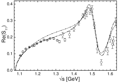
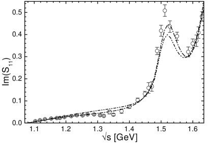
Figure 1: Effect of the chirally symmetric (calculation C-p-$\pi+$: dash-dotted) as compared to the chiral symmetry breaking (calculation C-p-$\pi/\!\!\!\!\,\chi+$: dash-double-dotted) $\sigma\pi\pi$ coupling in the $S_{11}$ $\pi N$ elastic partial wave. Left: real part; right: imaginary part. Data are from Ref. SM00 .

even extends up to the energy region of the second resonance ($\sqrt{s}\approx 1.65$ GeV).

The importance of the inclusion of a chirally symmetric $\sigma$ meson becomes especially obvious in the calculations, where the Pascalutsa spin-$\frac{3}{2}$ vertices (cf. Sec. II.1.2) are used. It turns out in the present model that the use of the chirally symmetric coupling is mandatory: With the nonderivative coupling, not even a fit to low-energy (up to $1.4$ GeV) $\pi N$ scattering has been possible. In Refs. feusti98 ; feusti99 , where the $\sigma$ meson was not included, it was shown that in particular the $\pi N$ $S_{31}$ partial wave can hardly be described when the spin-$\frac{1}{2}$ off-shell contributions of the $P_{33}(1232)$ were neglected. In the present calculations, however, we find that the inclusion of a chirally symmetric $\sigma$ meson exchange with a derivative $\sigma\pi\pi$ coupling allows the description of low-energy $\pi N$ elastic scattering even without this off-shell contributions, i.e., using the Pascalutsa prescription for the spin-$\frac{3}{2}$ vertices. From Fig. 2

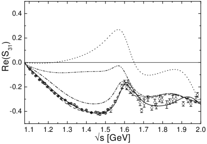
Figure 2: Effect of the $\sigma$ meson exchange on the real part of the $S_{31}$ partial wave in $\pi N$ scattering. P-p-$\pi+$ (solid line), P-p-$\pi+$ without $\sigma$ (dotted), C-p-$\pi+$ (dashed), C-p-$\pi+$ without $\sigma$ (dash-dot), C-p-$\pi+$ without $P_{33}(1232)$ (dash-double-dotted). Data are from Ref. SM00 .

it is obvious that a good description of the $S_{31}$ partial wave is indeed possible when the Pascalutsa couplings are used. At the same time it turns out that the $\sigma$ meson as a background contribution is enhanced as compared to when the conventional spin-$\frac{3}{2}$ couplings are used. This is not only manifested in the increase of the $\sigma$ couplings (see Table 4 below), but also the $t$-channel cutoff parameter $\Lambda_{t}$ (see Table 5 below) increases by a factor of $2$, meaning that the missing spin-$\frac{1}{2}$ off-shell background contributions of the spin-$\frac{3}{2}$ resonances are compensated by larger $t$-channel diagram contributions in the lower partial waves of all reaction channels. The resemblance of the calculations P-p-$\pi+$ without the $\sigma$ meson and C-p-$\pi+$ without the $P_{33}(1232)$ resonance also asserts the finding of Pascalutsa pasca01 and Pascalutsa and Tjon pascatjon that the two prescriptions for the spin-$\frac{3}{2}$ vertices become equivalent when additional background contributions are included, i.e., when the spin-$\frac{1}{2}$ off-shell contributions are reshuffled into other contributions. Similar observations concerning the importance of the inclusion of a $\sigma$ meson have also been made in the full BSE $\pi N\rightarrow\pi N$ model of Lahiff and Afnan lahiff . These authors have also allowed for the inclusion and neglect of the $P_{33}(1232)$ spin-$\frac{1}{2}$ off-shell contributions by using conventional and Pascalutsa $\pi N\Delta$ couplings. A ten times smaller $g_{\sigma NN}g_{\sigma\pi\pi}$ value in the conventional as compared to the Pascalutsa case was found. At the same time, the cutoff value of the $\sigma$ form factor in the conventional case has been much softer thus reducing the $\sigma$ contribution even further.

IV.2 $\pi N\rightarrow\pi N$

The resulting descriptions of the $\pi N$ elastic scattering partial waves are shown in Figs. 3 and 4

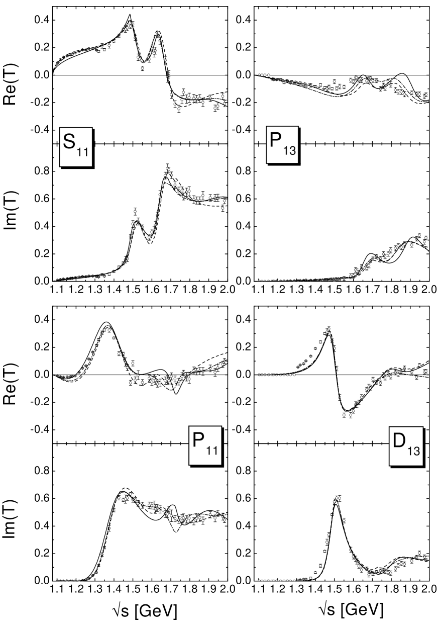
Figure 3: $\pi N\rightarrow\pi N$ partial waves for $I=\frac{1}{2}$. Calculation C-p-$\gamma+$: solid line, C-p-$\pi+$: dotted line, P-p-$\pi+$: dashed line. Data are from Ref. SM00 .

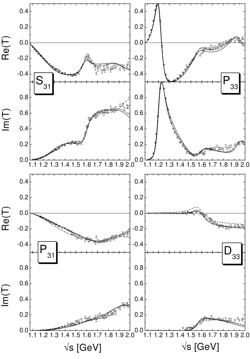
Figure 4: $\pi N\rightarrow\pi N$ partial waves for $I=\frac{3}{2}$. Notation and data as in Fig. 3.

in comparison with the continously updated single-energy partial wave SM00 analyses of the Virginia Polytechnic Institute (VPI) group, which greatly simplifies the analysis of experimental data within the coupled-channel formalism. Note that for those energies, where the single-energy solutions have not been available, the gaps have been filled with the energy-dependent solution of the VPI group. In most partial waves, the hadronic calculations using the Pascalutsa (P-p-$\pi+$) and conventional (C-p-$\pi+$) spin-$\frac{3}{2}$ vertices are very similar and equally well reproduce the $\pi N\rightarrow\pi N$ single-energy data points of SM00 . The largest differences are found in the

• $P_{11}$ wave around the $P_{11}(1710)$ resonance. Since there is no prominent structure in the $\pi N$ elastic scattering data, the width of this resonance is difficult to fix resulting in the different structures in Fig. 3. This also explains why the $P_{11}(1710)$ mass as given by the references in the Particle Data Group (PDG) review pdg ranges from about 1.69 to 1.77 GeV.

• $S_{11}$ wave around the $S_{11}(1650)$ resonance. Due to the missing off-shell contributions a more pronounced resonance behavior is needed in the Pascalutsa calculation to be able to describe the high-energy tails of the real and imaginary part.

• $S_{31}$ wave above 1.7 GeV. In this partial wave, it has turned out that adding a second resonance [besides the $S_{31}(1620)$] around 1.98 GeV improves the $\chi^{2}$ considerably in the Pascalutsa calculation. However, the same does not hold true for the other calculations, which consequently show less structure in the high-energy tail. See also Sec. V.3 below.

• $D_{13}$ wave above 1.8 GeV. In this partial wave, it has also turned out that adding a third resonance between 1.7 and 1.8 GeV, improves the $\chi^{2}$ considerably in the Pascalutsa calculation. Since the resulting resonance is rather narrow ($\Gamma_{tot}\approx 55$ MeV), the difference to the other calculations remains small and is only visible in the imaginary part between 1.7 and 1.8 GeV. See also Section V.3 below.

The calculation with the chiral symmetry breaking $\sigma$ contribution is not shown in Figs. 3 and 4 since it is very similar to the calculation C-p-$\pi+$; the main differences are contained in the low-energy tails of the spin-$\frac{1}{2}$ partial waves and especially in the $S_{11}$ wave, see Fig. 2 above.

For the extension of the model up to 2 GeV it turns out to be essential to add a resonance in the $P_{13}$, $P_{31}$, and $P_{33}$ partial waves as compared to Refs. feusti98 ; feusti99 . This is in line with Manley and Saleski manley92 , who found additional states around 1.88, 1.75, and 2.01 GeV, respectively. Without these resonances, those three partial waves cannot completely be described above 1.8 GeV in our model; see also Refs. feusti98 ; feusti99 . However, in the $P_{I3}$ waves, the new resonances are at the boundary of the energy range of the present model. This means that their properties cannot be extracted with certainty, but in both partial waves there is a clear indication for an additional contribution. See also Sec. V.3 below.

The most striking differences between the global and the purely hadronic fits can be seen in the low-energy tails of the $S_{11}$ and $P_{11}$ waves, which in the latter case is accompanied by an increase of the mass and widths of the $P_{11}(1440)$. While in the hadronic calculations the threshold behavior of all $J=\frac{1}{2}$ partial waves is nicely reproduced, which also leads to $\rho NN$ couplings in line with the KSRF relation (see Sec. V.1.1 below), in the global calculation this description is inferior. The reason for this behavior can be found in the necessity of the reduction of the nucleon form factor cutoff $\Lambda_{N}$ in the global fits due the $E_{0+}^{p/n}$ multipoles, see also the discussion on pion photoproduction in PMII pm2 . Thereby the low-energy interference pattern in $\pi N$ scattering between the $\rho$ meson and the nucleon is misbalanced and deteriorates in comparison with the hadronic fits. Moreover, the resonant structure due to the $P_{13}(1900)$ in the $P_{13}$ wave turns out to be more pronounced in the global fits as compared to the hadronic calculations. This is a consequence of the necessity of an enhanced $P_{13}$ contribution in the $\omega N$ production mechanism, see Sec. IV.7. In the isospin-$\frac{3}{2}$ partial waves, there is hardly any difference between the hadronic and the global fit results. The reason is that the $I=\frac{3}{2}$ resonances only contribute to pion and $K\Sigma$ photoproduction, and are hence not submitted to that many additional constraints of the photoproduction data as the isospin-$\frac{1}{2}$ resonances.

For a detailed discussion of the individual resonance contributions to the partial waves and the discrepancies in the $D_{13}$ partial wave below $1.45$ GeV, see Sec. V.3 below.

IV.3 $\pi N\rightarrow 2\pi N$

Manley et al. manley84 have performed a partial-wave analysis of pion-induced two-pion production on the nucleon taking into account the two-pion isobar states $\pi\Delta$, $\rho N$, $\sigma N$, and $\pi N^{*}(1440)$. Since in our model only one effective two-pion state ($\zeta N$) is included, where $\zeta$ is an artificial isovector-scalar meson, it is not possible to compare our calculation to the partial waves extracted in Ref. manley84 for the individual $2\pi N$ final states. To get a handle on the strength of the $2\pi N$ flux in the various partial waves, we use as experimental input the $\pi N\rightarrow 2\pi N$ partial-wave cross sections defined by

$$\sigma^{IJP}=\frac{4\pi}{\>\>\!\!{\mathrm{k}}^{2}}\sum_{\lambda,\lambda^{\prime}}(J+\mbox{$\frac{1}{2}$})\left|{\mathcal{T}}_{\lambda^{\prime}\lambda}^{IJP}\right|^{2}$$

that were also extracted in Ref. manley84 . These cross sections correspond to the sum of all individual $2\pi N$ fluxes for one partial wave, thus representing the total $2\pi N$ inelasticity. As a consequence of modeling the $2\pi N$ state by a two-body state within our model, one cannot expect that all details of these data can be described within the model. In particular, the threshold and phasespace behavior is different from the individual three-body final states. However, even with the assumption that the $\zeta$ meson only couples to resonances (see Sec. II.1.1, the $2\pi N$ flux is well reproduced in most partial waves up to $J=\frac{3}{2}$; see Fig. 5.

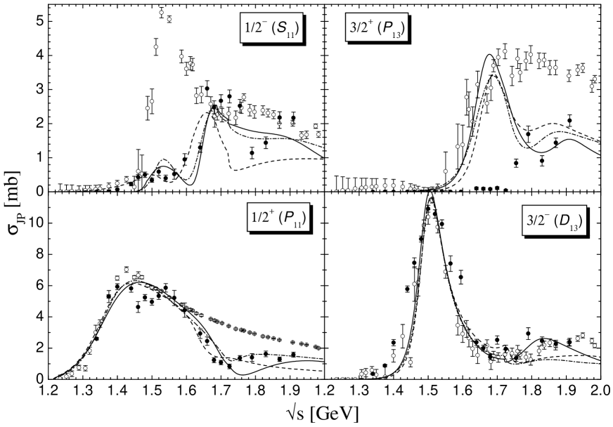
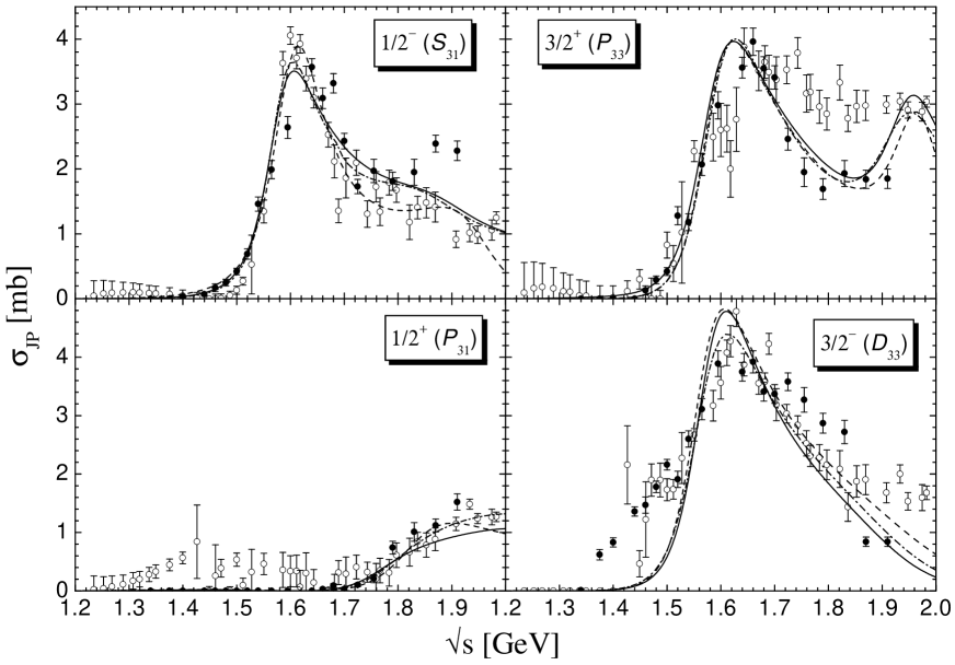
Figure 5: $\pi N\rightarrow 2\pi N$ partial-wave ($J^{P}$) cross sections for $I=\frac{1}{2}$ (upper panel) and $I=\frac{3}{2}$ (lower panel). The solid dots ($\bullet$) are taken from Ref. manley84 , the open dots ($\circ$) are the inelastic $\pi N\rightarrow\pi N$ partial-wave cross sections extracted from the VPI analysis SM00 . Notation as in Fig. 3.

This indicates that the pion-induced $2\pi N$ production is indeed dominated by baryon resonances. Since the $2\pi N$ final state clearly dominates all partial-wave inelasticities besides $S_{11}$, $P_{11}$, and $P_{13}$ (see below), cf. Fig. 5, the qualitative description of this channel is mandatory in a unitary model. The various calculations for the $2\pi N$ partial-wave cross sections are very similar in all partial waves, with the exception of the $S_{11}$ wave. There, the Pascalutsa calculation results in a largely decreased $S_{11}$ $2\pi N$ production above 1.7 GeV, below the $2\pi N$ production data. Although the $S_{11}$ $\omega N$ partial-wave cross section is increased simultaneously by about 0.5 mb as compared to the conventional calculations, the resulting total inelasticity is still reduced, see Fig. 6.

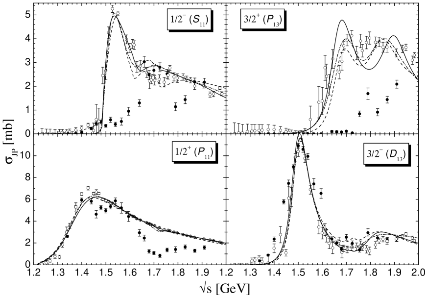
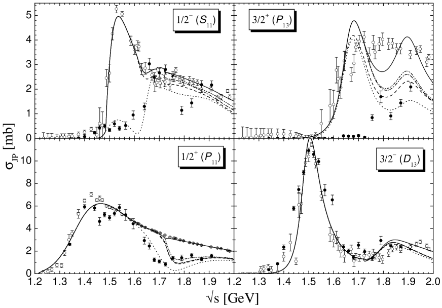
Figure 6: Inelastic partial-wave cross sections of $\pi N\rightarrow\pi N$ for $I=\frac{1}{2}$. Data as in Fig. 5. Upper panel: Notation as in Fig. 3. Lower panel: Decomposition of the inelasticities for calculation C-p-$\gamma+$. Partial-wave cross section of $2\pi N$: dotted, $+\eta N$: dashed, $+K\Lambda$: dash-dotted, $+K\Sigma$: dash-double-dotted, total ($+\omega N$): solid line.

All calculations show a kink structure in the $S_{11}$ and the $D_{13}$ $2\pi N$ flux at the $K\Sigma$ and the $\omega N$ thresholds, respectively, indicating that $2\pi N$ flux is moved to the corresponding channels.

The largest changes in the $2\pi N$ production upon inclusion of the photoproduction data can be observed in the $P_{11}$ and $D_{13}$ waves above the $\omega N$ threshold. The inclusion of the very precise preliminary $\omega N$ photoproduction data of the SAPHIR Collaboration barthom requires that inelastic contributions are moved from $2\pi N$ to $\omega N$ in the $P_{11}$ wave and vice versa in the $D_{13}$ case. This can also be seen in the dramatic change of the total $\pi N\rightarrow\omega N$ cross section behavior when the photoproduction data are included, see Fig. 15 below. Otherwise, similarly to the $\pi N\rightarrow\pi N$ case, also the $2\pi N$ production is only slightly changed by the inclusion of the photoproduction data. A small, but interesting change can, however, be observed in the high energy tail of the $P_{31}$ and $P_{33}$ waves, which can be traced back to the shift of inelasticity caused by $K\Sigma$ from $P_{33}$ in the hadronic calculations to $P_{31}$ in the global calculations; see also Sec. IV.6.

The only obvious discrepancy between the calculated $2\pi N$ partial-wave cross sections and the Manley et al. manley84 data is given in the $P_{13}$ partial wave. In the energy region between 1.55 and 1.72 GeV the inelasticity increases up to 4 mb in line with the calculated $2\pi N$ cross section, while the measured $2\pi N$ cross section is still zero. At the same time the total cross sections from all other open inelastic channels ($\eta N$, $K\Lambda$, and $K\Sigma$) add up to significantly less than $4$ mb. This indicates that either the extracted $2\pi N$ partial-wave cross section is not correct in the $P_{13}$ partial wave or another inelastic channel (i.e., an additional $3\pi N$ channel) gives noticeable contributions to this partial wave. The same problem with the $P_{13}$ inelasticity has also been observed in a resonance parametrization of $\pi N\rightarrow\pi N$ and $\pi N\rightarrow 2\pi N$ by Manley and Saleski manley92 . Since this is the only partial wave where such a large discrepancy is observed, no additional final state is introduced in the present model, but instead, we have largely increased the error bars of the $2\pi N$ data points in this energy region. However, it would be desirable to account for $3\pi N$ contributions in future investigations by the inclusion of, e.g., a $\rho\Delta$ final state. This might also clarify whether there is a missing ($3\pi N$) contribution in the $P_{33}$ wave above 1.7 GeV, see Fig. 5 and Sec. V.3 below. So far, no analysis has given such a contribution.

In addition, there is the same problem as in $\pi N$ scattering with the description of the rise of the $2\pi N$ production in the $D_{I3}$ waves, i.e. in the $D_{13}$ wave below $1.45$ GeV and in the $D_{33}$ wave below $1.55$ GeV, see Fig. 5. This effect is probably due to the effective description of the $2\pi N$ state in the present model; see the detailed discussion in Sec. V.3 below.

It is interesting to note that the inelasticities of $\pi N\rightarrow\pi N$ scattering only enter the fitting procedure indirectly, since the real and imaginary part of the partial waves are the input for the calculations. Therefore the very good description of the partial-wave inelastic $\pi N$ cross sections in all calculations, see the upper panel in Fig. 6, is an outcome of summing up the partial-wave cross sections of all other $\pi N$-induced channels. Note that the inelasticities for the $I=\frac{3}{2}$ partial waves are not shown for the different calculations, since due to the smallness of the $K\Sigma$ contributions, the results are almost identical to the $2\pi N$ partial-wave cross sections. From Figs. 5 and 6 we can thus deduce that not only is the PWD of all inelastic channels on safe grounds, but also that all important channels for the considered energy region are included. At the same time, this shows that the experimental data on the various reactions are indeed compatible with each other, in particular no significant discrepancy between the measured $\pi N$ inelasticity and the sum of all partial-wave cross sections is observed. The only exceptions are the aforementioned indications for missing ($3\pi N$) contributions in the $P_{I3}$ waves.

Note also that the inclusion of the photoproduction data only slightly changes the total inelasticities of the individual partial waves. The only noticeable differences between the hadronic and global calculation is a decrease of the $S_{11}$ inelasticity between $1.6$ and $1.7$ GeV, and an increase in the $P_{13}$ inelasticity around the $P_{13}(1720)$.

In the lower panel of Fig. 6, the decomposition of the $\pi N$ inelasticity of the best global fit C-p-$\gamma+$ is shown. It can be deduced that the $\pi N$ inelasticities are made up in all partial waves mainly by the $2\pi N$ channel. This also allows us to deduce that the Manley $2\pi N$ data manley84 are in line with the $\pi N$ inelasticitis of the VPI analysis SM00 . The only contradictions can be observed in the $D_{13}$ wave at 1.6, 1.7, and 1.8 GeV, in the $S_{31}$ wave above 1.85 GeV and the $D_{33}$ wave between 1.7 and 1.85 GeV.

Besides the $2\pi N$ channel, there are in all partial waves important contributions to the inelasticities from other channels. Thus the necessity of the inclusion of a large set of final states in a coupled-channel calculation can be seen in various partial waves:

• In the $S_{11}$ wave there is the well known $\eta N$ contribution around the $S_{11}(1535)$. Note that the $\eta N$ inelasticity also exhibits a second hump, which is due to the interference between the $S_{11}(1535)$ and the $S_{11}(1650)$ resonances, although the latter only has a very small $\eta N$ width. See also Sec. IV.4.

• In the $P_{11}$ wave there is also an important contribution by the large $\eta N$ and $\omega N$ widths of the $P_{11}(1710)$ resonance. This contrasts previous analyses feusti99 ; manley92 , where this contribution has been assigned to the $K\Lambda$ channel.

• The $P_{13}$ wave contains important contributions from $\eta N$ and $\omega N$ as well, where the first one stems from the $P_{13}(1900)$ resonance, while the latter one consists of important contributions from both $P_{13}$ resonances.

• The $D_{13}$ wave is also fed by a smoothly increasing $\omega N$ contribution.

The other final states, i.e., the associated strangeness channels $K\Lambda$ and $K\Sigma$, are only of minor importance for the $\pi N$ inelasticities. While both give visible contributions in the $S_{11}$ wave, $K\Lambda$ also shows up in the $P_{13}$ and $K\Sigma$ in the $P_{11}$ wave.

IV.4 $\pi N\rightarrow\eta N$

In the first coupled-channel effective Lagrangian model on $\eta N$ production by Sauermann et al. sauermann , this channel has been described by a pure $S_{11}$ mechanism for energies up to $\sqrt{s}=1.75$ GeV. As Fig. 7 shows,

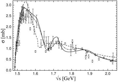
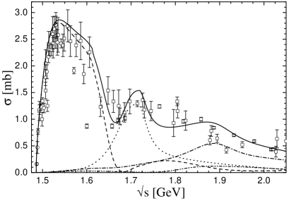
Figure 7: $\pi^{-}p\rightarrow\eta n$ total cross section. The new threshold data from Ref. morrison are denoted by $\circ$, all other data (see Ref. feusti98 ) by $\Box$. Left: Results from the different calculations. Notation as in Fig. 3. Right: Partial-wave decomposition of the total cross section for the calculation C-p-$\gamma+$. $J^{P}=\frac{1}{2}^{-}(S_{11})$: dashed line; $\frac{1}{2}^{+}(P_{11})$: dotted line; $\frac{3}{2}^{+}(P_{13})$: dash-dotted line; $\frac{3}{2}^{-}(D_{13})$: dash-double-dotted line (in brackets the $\pi N$ notation is given). The sum of all partial waves is given by the solid line.

the $\pi N\rightarrow\eta N$ reaction is indeed dominantly composed of the $S_{11}$ contribution due to the $S_{11}(1535)$, however, only for energies up to $\approx 1.65$ GeV. Due to its large $\eta N$ width the $P_{11}(1710)$ dominates in the following energy window up to $1.8$ GeV, while for the highest energies, the $P_{13}(1900)$ resonance is strongest. The double hump structure in the $S_{11}$ contribution is due to the destructive interference between the $S_{11}(1535)$ and $S_{11}(1650)$ resonances, even though the latter one has a much smaller $\eta N$ decay ratio. This interference pattern exhibits maximal destructive interference at the $S_{11}(1650)$ resonance position, while above 1.7 GeV the $S_{11}$ contribution is resurrected.

The importance of the $P_{11}(1710)$ contribution has also been found in the resonance parametrization of $\pi N\rightarrow\pi N$ for $I=\frac{1}{2}$ and $\pi N\rightarrow\eta N$ by Batinić et al. batinic , who extracted a total width for this resonance of about 120 MeV and an $\eta N$ decay ratio of almost 90%. However, in contrast to the results of these authors, we also find in the present calculation important contributions of the $P_{13}(1900)$ at higher energies. These contributions are in line with the observed differential cross section at higher energies, see Fig. 8.

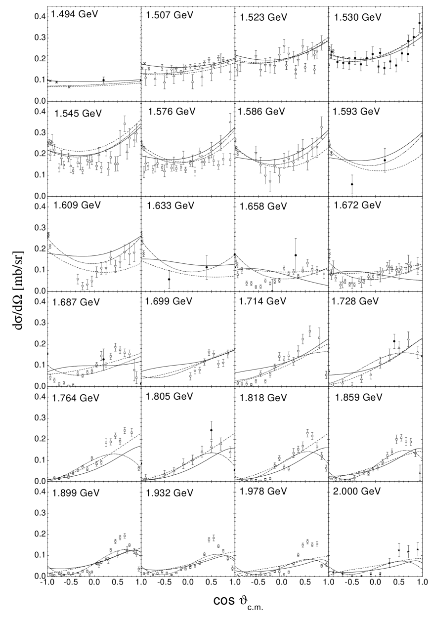
Figure 8: $\pi^{-}p\rightarrow\eta n$ angle-differential cross section. For the data references, see Refs. feusti98 and gregiphd . Notation as in Fig. 3.

However, some deviations in the differential cross section behavior between calculation and experimental data are observed and the angular structure cannot be fully described. But one has to note, that at higher energies, there are almost only experimental data available from Brown et al. brown ($\Box$ in Fig. 8), which enter with enlarged error bars due to problems with the momentum calibration in the experiment, see Refs. batinic ; feusti98 . Hence these discrepancies hardly influence the fitting procedure and the resulting $\chi^{2}$ is still rather good. Since at energies above 1.8 GeV, there are almost only data available from Brown et al. brown , a reliable decomposition in this region can only be achieved after the inclusion of the $\eta N$-photoproduction data.

In this reaction channel, large differences between the Pascalutsa and conventional calculations are observed. This is related to the visible differences in the $S_{11}$ $\pi N\rightarrow\pi N$ partial wave, since this partial wave constitutes the largest contribution in the $\eta N$ production mechanism. An obvious difference is that the Pascalutsa calculation results in less angular structure of the angle-differential cross section at higher energies, however, influencing the resulting $\chi^{2}$ only to a minor degree, see above. On the other side, the inclusion of the photoproduction data hardly changes the total cross section behavior. Only the $P_{11}(1710)$ contribution is slightly emphasized, which also leads to the observed differences in the differential cross section. Moreover, the $\omega N$ threshold effect in the $P_{11}$ wave can be clearly observed in calculation C-p-$\gamma+$ and C-p-$\pi+$.

IV.5 $\pi N\rightarrow K\Lambda$

$K\Lambda$ production turns out to be a channel which is very sensitive to rescattering effects. The inclusion of the $K\Sigma$ and $\omega N$ final states strongly alters the total cross section in this reaction, especially in the hadronic calculations, see Fig. 9.

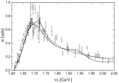
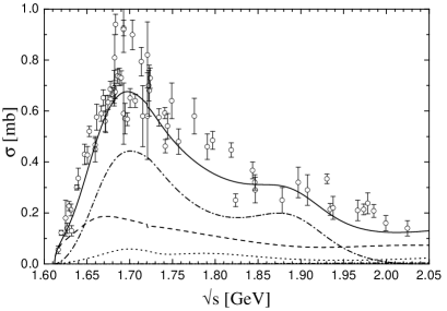
Figure 9: $\pi^{-}p\rightarrow K^{0}\Lambda$ total cross section. For the data references, see Ref. feusti98 . Left: Results of the different calculations. Line code as in Fig. 3. Right: Partial-wave decomposition of the total cross section. Notation as in Fig. 7.

In both of the displayed hadronic calculations, the $K\Sigma$ channel leads to a kink in the $S_{11}$ partial wave, which has already been observed in the coupled-channel chiral SU(3) model of Ref. nobby including only $S$ and $P$ waves, while the $\omega N$ channel strongly influences the $P$ waves.

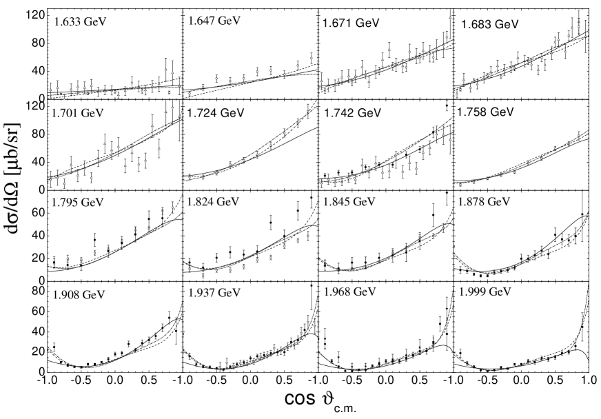
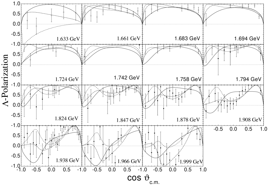
Figure 10: $\pi^{-}p\rightarrow K^{0}\Lambda$ angle- differential cross sections (upper panel) and polarization measurements (lower panel). For the data references, see Refs. feusti98 ; gregiphd . Notation as in Fig. 3.

The inclusion of these coupled-channel effects and of the $P_{13}(1900)$ resonance are major improvements as compared to Refs. feusti98 ; feusti99 . There, these mechannisms were not included and thus the $K\Lambda$ channel was not subjected to any threshold effect and the peaking behavior around 1.7 GeV had to be fully described by the $P_{11}(1710)$ resonance. In the extended model space, this resonancelike behavior is mainly caused by the $P_{13}(1720)$ resonance, but also influenced by the opening of these two channels.

The $S$ wave behavior in the Pascalutsa calculation P-p-$\pi+$ differs above 1.65 GeV from that in the conventional calculation C-p-$\pi+$ (see Sec. IV.2 and Fig. 3). The largest differences between these calculations can thus be observed in the $S_{11}$ wave contribution, which is more pronounced in the Pascalutsa calculation giving rise to a slightly different behavior at the lowest energies and at the $K\Sigma$ threshold. The coupled-channel effects become less obvious once the photoproduction data are included. In the global calculation C-p-$\gamma+$ the $S_{11}$ and $P_{13}$ waves are only slightly influenced by the $\omega N$ threshold, while the $K\Sigma$ threshold effect has completely vanished. Note that the $P_{13}$ wave dominates over almost the complete considered energy region. The second most important part comes from the $S_{11}$ staying almost constant in the upper energy range, while close to threshold, a slight peak caused by the $S_{11}(1650)$ is visible.

Although the new $P_{13}(1900)$ only has a small $K\Lambda$ width, it improves the description of the reaction significantly due to rescattering, similarly to the $S_{11}(1650)$ resonance in $\pi N\rightarrow\eta N$. Thus the $P_{13}(1900)$ gives rise to a good description of the angle differential observables, while in Ref. feusti98 only contributions from the $S_{11}(1650)$ and $P_{11}(1710)$ resonances were found. The improvement becomes most visible in the high energy region, where the full angular structure of the cross section and polarization of the $K\Lambda$ channel can be described, see Fig. 10. Especially for a description of the upward bending behavior of the differential cross section at backward angles at the highest energies, the inclusion of the $P_{13}(1900)$ turns out to be important. Note that due to the change of the $K_{0}^{*}$ coupling (cf. Table 4), the extreme forward peaking behavior of the hadronic calculations is not visible any more in the global calculation.

The polarization data hardly influence the determination of the parameters due to the large error bars, see Fig. 10. However, all calculations give a good description of the angular and energy dependent structure, in particular the pure positive polarization for lower energies and the change to negative values for the backward angles at higher energies.

IV.6 $\pi N\rightarrow K\Sigma$

Due to the isospin structure of the $K\Sigma$ final state, the $\pi N\rightarrow K\Sigma$ channel is similar to $\pi N$ elastic scattering. The reaction process is determined by two isospin amplitudes ($I=\frac{1}{2}$ and $I=\frac{3}{2}$), while data have been taken for the three charge reactions $\pi^{+}p\rightarrow K^{+}\Sigma^{+}$, $\pi^{-}p\rightarrow K^{0}\Sigma^{0}$, and $\pi^{-}p\rightarrow K^{+}\Sigma^{-}$. Since the first reaction is purely $I=\frac{3}{2}$, it allows a stringent test of the $I=\frac{3}{2}$ (resonance) contributions in the present model, while the other two are a mixture of $I=\frac{1}{2}$ and $I=\frac{3}{2}$ contributions [see Eqs. (126)]. Within our model it is possible to describe all three charge reactions with approximately the same quality, see Table 3,

Fit	Total $\chi^{2}_{\pi\Sigma}$	$\chi^{2}(\pi^{-}p\rightarrow K^{0}\Sigma^{0})$	$\chi^{2}(\pi^{-}p\rightarrow K^{+}\Sigma^{-})$	$\chi^{2}(\pi^{+}p\rightarrow K^{+}\Sigma^{+})$
C-p-$\pi+$	1.97	2.14	1.85	1.97
C-p-$\pi-$	2.37	3.08	1.86	1.96
P-p-$\pi+$	2.93	3.34	1.67	3.01
P-p-$\pi-$	2.80	3.04	1.90	2.91
C-p-$\pi/\!\!\!\!\,\chi+$	2.48	2.63	2.29	2.42
C-t-$\pi+$	2.42	3.18	1.61	2.05
C-t-$\pi-$	2.48	3.67	1.92	1.66
C-p-$\gamma+$	2.97	2.76	2.06	3.45
C-p-$\gamma-$	3.94	4.06	4.90	3.53

Table 3: Resulting $\chi^{2}$ of the various fits for the three different charge reactions of $\pi N\rightarrow K\Sigma$.

corroborating the isospin decomposition of the $K\Sigma$ channel in the present calculation. From the total cross section behavior, shown in Fig. 11,

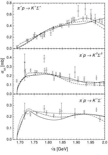
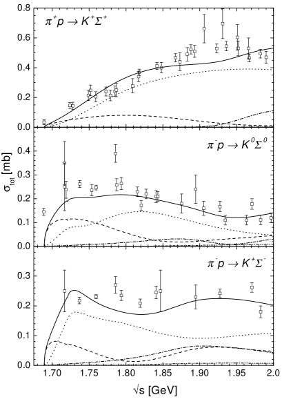
Figure 11: $\pi N\rightarrow K\Sigma$ total cross sections for the different charge reactions. Notation as in Fig. 3. For the data references, see Refs. gregi ; gregiphd . Left: Results of the different calculations. Notation as in Fig. 3. Right: Partial-wave decomposition of the total cross section for the calculation C-p-$\gamma+$. $J^{P}=\frac{1}{2}^{-}(S_{I1})$: dashed line; $\frac{1}{2}^{+}(P_{I1})$: dotted line; $\frac{3}{2}^{+}(P_{I3})$: dash-dotted line; $\frac{3}{2}^{-}(D_{I3})$: dash-double-dotted line. The sum of all partial waves is given by the solid line.

one deduces, that the threshold behavior of the reactions with $I=\frac{1}{2}$ contributions is influenced by a strong $S_{11}$ wave, arising from the $S_{11}(1650)$ just below the $K\Sigma$ threshold, and $P_{I1}$-wave dominance for increasing energies, which stem from the $P_{31}(1750)$ and in particular the $P_{11}(1710)$. However, the $P_{13}(1900)$ is also visible in the $K^{+}\Sigma^{-}$ channel. In the pure $I=\frac{3}{2}$ reaction the $S$ wave importance is largely reduced, and the $P$ waves dominating over the complete energy range. Note that the $J^{P}=\frac{3}{2}^{-}$ waves do not give any noticeable contribution to the cross sections, see also below. In the hadronic reactions it turns out that the main contribution to the $I=\frac{3}{2}$ channel comes from the $P_{33}(1920)$, however, the inclusion of the photoproduction data moves this strength over to the $P_{31}(1750)$; see also Sec. IV.3 above. A similar observation is made in the $I=\frac{1}{2}$ sector, where strength is also moved over from the $P_{13}$ to the $P_{11}$ waves and the latter one is realized in a large $P_{11}(1710)$ $K\Sigma$ width.

These contributions result in a very good description of the differential cross sections and polarization measurements for all three reactions, see Figs. 12 – 14.

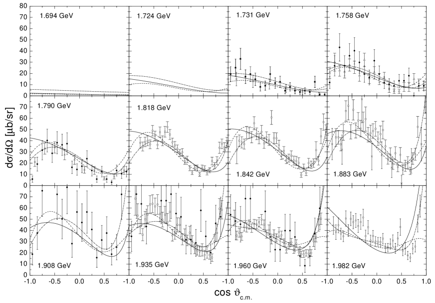
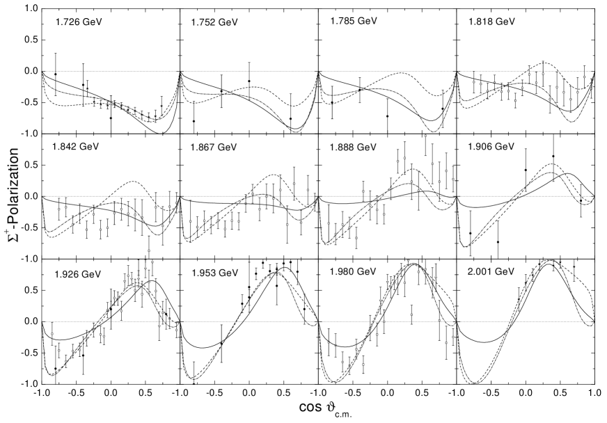
Figure 12: $\pi^{+}p\rightarrow K^{+}\Sigma^{+}$ differential cross sections (upper panel) and $\Sigma^{+}$-polarization measurements (lower panel). Notation as in Fig. 3. For the data references, see Refs. gregi ; gregiphd .

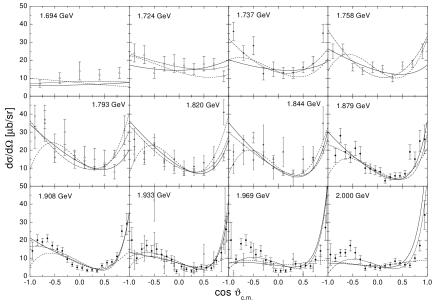
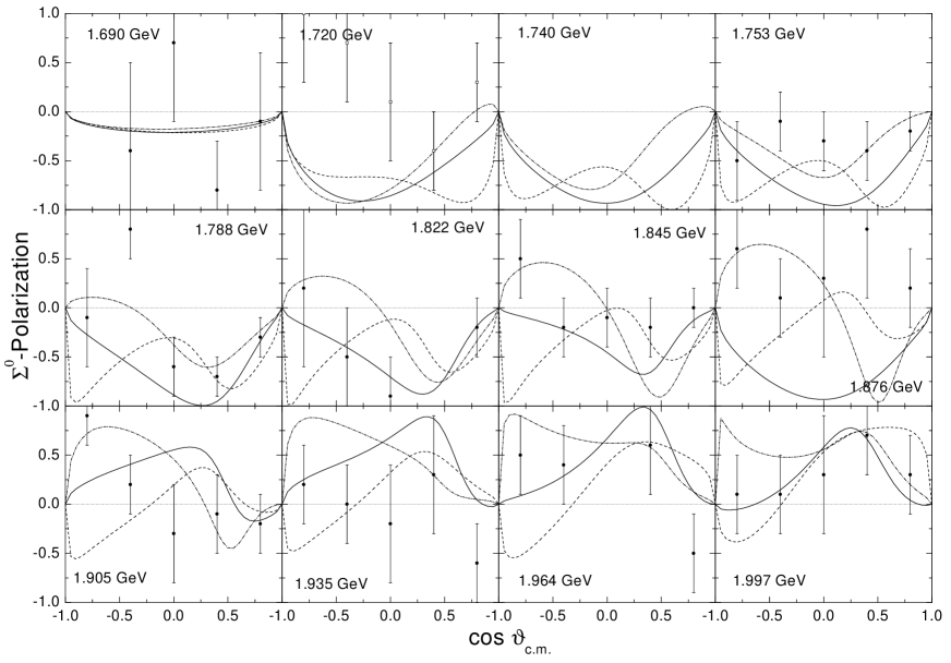
Figure 13: $\pi^{-}p\rightarrow K^{0}\Sigma^{0}$ differential cross sections (upper panel) and $\Sigma^{0}$-polarization measurements (lower panel). Notation as in Fig. 3. For the data references, see Refs. gregi ; gregiphd .

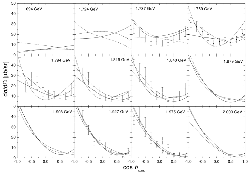
Figure 14: $\pi^{-}p\rightarrow K^{+}\Sigma^{-}$ angle-differential cross section. Notation as in Fig. 3. For the data references, see Refs. gregi ; gregiphd .

As pointed out above, the three reaction channels, which are built up by only two isospin amplitudes, allow for strong constraints on the partial-wave decomposition of the $K\Sigma$ production. Within our model the full angular structure of all three charge reactions can be well described, while in the SU(3) model of Ref. nobby problems have been observed with the description of the backward peaking behavior of the angle differential $\pi^{-}p\rightarrow K^{+}\Sigma^{-}$ cross section at higher energies. This large difference to the other two charge reactions, who both show a forward peaking behavior in this energy range, can, however, be easily explained with the help of the $t$-channel meson contributions of $K^{+}$ and $K_{0}^{*}$. Since both are $I=\frac{1}{2}$ particles, they can only contribute to $\pi^{-}p\rightarrow K^{0}\Sigma^{0}$ and $\pi^{+}p\rightarrow K^{+}\Sigma^{+}$, but not to $K^{+}\Sigma^{-}$ production, which consequently tends to small values at forward angles. The lack of $t$-channel contributions also explains the good result of the calculation C-t-$\pi+$ for $\pi^{-}p\rightarrow K^{+}\Sigma^{-}$, where the form factor $F_{t}$ has been used, although this form factor leads in general to worse results (see Tables 2 and 3). On the other hand, the very good result of C-t-$\pi-$ for $\pi^{+}p\rightarrow K^{+}\Sigma^{+}$ has to be compensated by a much worse $\pi^{-}p\rightarrow K^{0}\Sigma^{0}$ result.

This is also related to the observed difference between the Pascalutsa and the conventional calculations in the differential cross section of $K\Sigma$ production at higher energies. The large forward peaking behavior for higher energies in the $K^{+}\Sigma^{+}$ and $K^{0}\Sigma^{0}$ production cannot be described in the Pascalutsa calculation. Due to the lack of the spin-$\frac{3}{2}$ offshell contributions, in this calculation a larger cutoff value $\Lambda_{t}$ is extracted, thus giving rise to more background contributions over the complete angle and energy range. At the same time, a description of the forward peaking behavior at high energies requires large couplings to the $t$-channel mesons, but in the Pascalutsa calculations this would spoil the agreement at backward angles and lower energies. Consequently, the most striking differences between the Pascalutsa and conventional calculations are found in the high-energy region. For more details on the $t$-channel form factors and couplings, see the discussion in Secs. V.1.2 and V.1.3.

While the polarization measurements for $\pi^{-}p\rightarrow K^{0}\Sigma^{0}$ hardly influence the parameter extraction due to the large error bars, the measurements for $\pi^{+}p\rightarrow K^{+}\Sigma^{+}$ largely constrain the $I=\frac{3}{2}$ contributions, see Figs. 12 and 13. The change of negative to positive polarization values at forward angles with increasing energy, peaking around $\cos\vartheta\approx 0.4$ is nicely described as a result of the $P_{33}(1920)$ contribution, confirming the strong necessity of $K\Sigma$ flux in the $P_{33}$ partial wave at higher energies. Note further that although the contribution of the $D_{33}(1700)$ to the total cross section is negligible (cf. Fig. 11), it leads to the negative hump at $\cos\vartheta\approx 0.7$ in the $\Sigma^{+}$ polarization close to threshold, thus affirming the necessity of subthreshold contributions. Polarization measurements of comparable quality for the reactions with isospin-$\frac{1}{2}$ contributions would be very interesting for testing the importance of the various resonance contributions, since due to the large error bars, the different calculations for the polarization measurement in $\pi^{-}p\rightarrow K^{0}\Sigma^{0}$ result in a quite different behavior. The only common characteristic of the different calculations in the $K^{0}\Sigma^{0}$ polarization is caused by the $D_{33}(1700)$ and $P_{33}(1920)$ resonances, enforcing the change from negative polarization values at low energies to positive values at high energies in the forward region.

IV.7 $\pi N\rightarrow\omega N$

As can be seen from Fig. 15 the $\omega N$ channel,

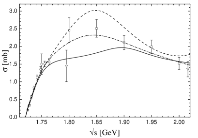
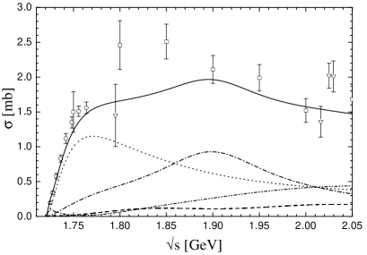
Figure 15: $\pi^{-}p\rightarrow\omega n$ total cross section. For the data references, see Refs. gregi ; gregiphd . Left: Results of different calculations. Line code as in Fig. 3. Right: Partial-wave decomposition of the total cross section. $J^{P}=\frac{1}{2}^{-}$: dashed line; $\frac{1}{2}^{+}$: dotted; $\frac{3}{2}^{+}$: dash-dotted; $\frac{3}{2}^{-}$: dash-double-dotted.

which strongly influences all other reactions, cannot be completely fixed by using the pion-induced data alone. While in the hadronic calculations C-p-$\pi+$ and P-p-$\pi+$, the total cross section is dominated by a $J^{P}=\frac{3}{2}^{-}$ wave, resonating below 1.85 GeV and accompanied by a strong $\frac{3}{2}^{+}$ wave, this picture is changed once the much more precise $\omega N$ photoproduction data from the SAPHIR Collaboration barthom are included. In the global calculation, the $\frac{1}{2}^{+}$ and $\frac{3}{2}^{+}$ waves dominate up to energies of 2 GeV. The $P_{11}(1710)$ leads to the peaking in the $\frac{1}{2}^{+}$ wave around 1.76 GeV, while the $P_{13}(1900)$ gives rise to the peaking behavior of the $\frac{3}{2}^{+}$ contribution around 1.9 GeV, see Fig. 15. This decomposition leads to a slower increase of the total cross section at energies above 1.745 GeV; a property which is also indicated by the precise Karami total cross section data karami . This is in contrast to our findings in Ref. gregi , where a dominant $\frac{3}{2}^{-}$ contribution has been extracted because the more precise photoproduction data have not been considered simultaneously. The comparison of this result with the coupled-channel model of Lutz et al. lutz is especially interesting, because there, $\pi N\rightarrow\omega N$ is described by a pure $\frac{3}{2}^{-}$ production mechanism. This is due to the fact that in the model of Ref. lutz no $P$ wave contributions are included. These authors’ findings seem to lead to an overestimation of the $\pi N$ inelasticity in the $\frac{3}{2}^{-}$ ($D_{13}$) channel, which just starts overshooting the experimental data at the $\omega N$ threshold. Unfortunately, they do not compare their calculation to the angle-differential Karami cross section karami , which would allow for a further evaluation of the quality of their calculation. There has also been a single-channel analysis on $\pi N\rightarrow\omega N$ by Titov et al. titov . These authors have extracted dominant contributions from the subthreshold $S_{11}(1535)$, $S_{11}(1650)$, and $P_{11}(1440)$ resonances, which only give minor contributions in the present calculation. These authors also neglected the $P_{11}(1710)$ and resonances beyond the $P_{13}(1720)$, both of which turn out to be most important in the present calculation.

This once again shows the necessity of the inclusion of photoproduction data for a reliable analysis of resonance properties, especially in channels (as the $\omega N$ production), where only few precise pion-induced data are available.

The differential cross section shows an almost flat behavior close to threshold, see Fig. 16, even for the global calculation dominated by $P$ waves.

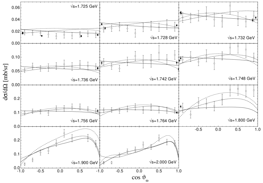
Figure 16: $\pi^{-}p\rightarrow\omega n$ angle-differential cross section. Line code as in Fig. 3. For the data references, see Refs. gregi ; gregiphd .

To get a handle on the angle-differential structure of the cross section for higher energies ($\sqrt{s}\geq 1.8$ GeV) we have used the corrected cosine event distributions given in Ref. danburg to also extract differential cross sections with the help of the given total cross sections. While the differential cross section at forward angles is almost constant above 1.8 GeV, the backward cross section decreases. These data points strongly constrain the nucleon $u$-channel contribution thereby restricting the $\omega NN$ coupling constants, and the downbending behavior is best described by the global fit. At these energies also the forward peaking behavior becomes visible which is due to the $t$-channel $\rho$ meson exchange. This contribution is also the reason why the forward peaking behavior is more pronounced in the Pascalutsa calculation. Although the extracted $\rho NN$ coupling is smaller than in the other calculations, the cutoff value $\Lambda_{t}$ (cf. Tables 4 and 5 below) is much larger than in the other calculations resulting in an effectively larger contribution, see also the discussion in Secs. V.1.2 and V.1.3 below.

It should also be noted that the $\omega N$ parameters are not constrained by the $\omega N$ data points alone but also greatly influenced by the $\pi N$ inelasticities and cusp effects appearing in $\eta N$, $K\Lambda$, and $K\Sigma$ production due to the $\omega N$ threshold opening. Therefore the extracted partial-wave decomposition of $\pi N\rightarrow\omega N$ is on safe grounds, since all other channels and in particular the $\pi N\rightarrow\pi N$ partial waves and inelasticities and the pion-induced $2\pi N$ production are well described in the energy region above the $\omega N$ threshold. However, more precise cross section measurements at energies above $1.76$ GeV and polarization measurements of the $\pi N\rightarrow\omega N$ production would be the perfect tool to corroborate the present findings.

V Extracted Hadronic Parameters

V.1 Background contributions and $t$-channel form factors

The values of all Born and $t$-channel coupling constants, which have been varied during the calculation, are listed in Table 4.

$g$	value	$g$	value	$g$	value	$g$	value
$g_{NN\pi}$	12.85	$g_{NN\sigma}\cdot g_{\sigma\pi\pi}$	$22.92$	$g_{NN\rho}$	4.53	$\kappa_{NN\rho}$	1.47
	12.75		$25.14$		4.40		1.41
	12.77		$26.88$		5.59		1.51
	12.80		$39.16$		2.71		1.16
	13.01		$13.66$		2.21		1.30
$g_{NN\eta}$	0.10	$g_{NNa_{0}}$	$-70.60$	$g_{NN\omega}$	3.94	$\kappa_{NN\omega}$	$-0.94$
	0.12		$-45.82$		3.87		0.17
	0.06		39.56		4.06		0.48
	0.07		$-2.98$		3.90		0.59
	0.29		$8.60$		3.94		-0.90
$g_{N\Lambda K}$	$-12.20$	$g_{N\Lambda K_{0}^{*}}$	52.54	$g_{N\Lambda K^{*}}$	$-27.61$	$\kappa_{N\Lambda K^{*}}$	$-0.50$
	$-12.88$		$2.32$		$-28.29$		$-0.55$
	$-18.48$		$-25.56$		$-27.85$		$-0.36$
	$-14.35$		$2.36$		$3.10$		$0.01$
	$-11.53$		$-11.58$		$-5.86$		$-0.39$
$g_{N\Sigma K}$	2.48	$g_{N\Sigma K_{0}^{*}}$	$-52.30$	$g_{N\Sigma K^{*}}$	4.33	$\kappa_{N\Sigma K^{*}}$	$-0.86$
	1.56		$-54.44$		3.88		$-0.98$
	15.39		$65.28$		2.29		$0.40$
	12.44		$-2.14$		$-4.22$		$-0.33$
	2.50		$11.06$		$0.71$		$-0.11$

Table 4: Nucleon and $t$-channel couplings. First line: C-p-$\gamma+$; second line: C-p-$\gamma-$; third line: C-p-$\pi+$; fourth line: P-p-$\pi+$; fifth line: C-t-$\pi+$. The values for the $K_{1}$ meson are given for the global calculations C-p-$\gamma+$ and C-p-$\gamma-$.

Note that no other background parameters are used in the calculations, emphasizing the reduced freedom of the background in our model as compared to analyses driven by resonance models (see, e.g., Ref. vrana ).

V.1.1 Born couplings

Our values of $g_{\pi NN}$ are consistently lower than the values extracted by other groups, for example the value of $g_{\pi NN}=13.13$ from the VPI group SM00 . However, one has to keep in mind that the present calculation considers a large energy region using only one $\pi NN$ coupling constant, thereby putting large constraints through all production channels on this coupling and the threshold region only plays a minor role. For example in the global fits, the $\pi NN$ coupling is especially influenced by the $t$-channel pion exchange mechanism of $\omega N$ photoproduction, which is due to the restriction of using only one cutoff value $\Lambda_{t}$ for all $t$-channel diagrams.

For the other couplings of the nucleon to the pseudoscalar final state mesons, the situation in the pion-induced reactions is different. As found in previous analyses sauermann ; feusti98 ; feusti99 the $\eta NN$ coupling turns out to be very small and the precise value thus hardly influences the $\chi^{2}$ of $\eta N$ production. Also in $\pi N\rightarrow K\Lambda/K\Sigma$, the Born couplings are only of minor importance due to the large offshellness of the nucleon and the associated large reduction of its contributions by the hadronic form factor. For example, a doubling of the $KN\Lambda/\Sigma$ coupling constants keeping all other contributions fixed leads to a worsening in $\chi^{2}$ for $\pi^{-}p\rightarrow K^{0}\Sigma^{0}/K^{+}\Sigma^{-}$ of only about 10%, and for $\pi^{-}p\rightarrow K^{0}\Lambda$ of about 15%. This also explains, why the $NK\Sigma$ coupling extracted from the pion-induced data alone, always ends up to be large compared to SU(3) expectations. However, the situation changes drastically when the photoproduction data is included. As a result of gauge invariance, the importance of the Born diagrams is enhanced in the photoproduction reactions and allows to determine the Born couplings more reliably. The resulting relations between the Born couplings of our best global fit are actually close to SU(3) relations with $\alpha_{FD}=F/(F+D)\in[0.25;0.41]$ (see, e.g., Ref. dumbrajs ), which is around the value of $\alpha_{FD}\approx 0.35$ predicted by the Cabibbo-theory of weak interactions and the Goldberger-Treiman relation dumbrajs .

As has already been pointed out in Ref. gregi , the $\omega NN$ coupling constants have more influence on the angular dependent behavior of the pion-induced reaction process than the $NK\Lambda$ and $NK\Sigma$ couplings and can therefore be better fixed already in the hadronic fits, see Table 4. This is a result of the nucleon $u$-channel contribution, which strongly influences the behavior of the angle-differential cross section in the backward direction at higher energies, and explains why the resulting values for this coupling are very similar in all calculations. Note that a value $g_{\omega NN}\approx 4$ is extracted in our calculations, even though the same nucleon cutoff $\Lambda_{N}\approx 1$ GeV (see Table 5) is used for all final states, which is in contrast to the results found in single-energy analysis (see, e.g., Ref. titov ).

V.1.2 $t$-channel form factors

It is interesting to compare our value of $g_{\omega NN}\sim 4$ with, e.g., the value of $15.9$ which has been extracted in the Bonn-model for nucleon-nucleon scattering machleidt . In nucleon-nucleon scattering, the $\omega$ only contributes via $t$-channel exchange and thus its coupling is always modified by a form factor. The actual shape of the form factor and the kinematic region are thus of great importance for the applicability of the extracted coupling.

We have examined the influence of the form factor shape by performing calculations with two different form factors $F_{p}$ (12) and $F_{t}$ (13) for the $t$-channel exchanges. In Ref. feusti98 no significant differences in the resulting quality of the fits have been found, when either of the two form factors has been used and consequently, in Ref. feusti99 only calculations using $F_{t}$ have been performed. However, as Table 2 shows, this result is not valid any more for the extended channel space and kinematic region of the present model. The calculations C-t-$\pi\pm$, which use $F_{t}$ instead of $F_{p}$ as in C-p-$\pi\pm$, result in an overall description, which is worse by more than 10%, with the largest differences in the $\pi N\rightarrow\omega N$ reaction. This reaction differs from $\eta N$, $K\Lambda$, and $K\Sigma$, which have comparable $\chi^{2}$, in that respect, that in the $t$ channel the $\rho$ meson is exchanged. Since this exchange also contributes to $\pi N$ elastic scattering, the combination of coupling and form factor for the $NN\rho$ vertex is tested in two different reactions and thus in a wide kinematic region. As a result of the larger data base for $\pi N$ elastic scattering, the value of $g_{\rho NN}$ is adjusted to this reaction and there is no freedom left for $\pi N\rightarrow\omega N$. Since the calculations using $F_{p}$ can describe both reactions simultaneously, the form factor shape $F_{p}$ seems to be applicable to a wider kinematic region than $F_{t}$. Note that this finding is even fortified when we look at the global fits. There, no satisfying description of the experimental data using $F_{t}$ has been possible, see PMII pm2 . This comes about because of the quite different $q^{2}$ dependent behavior of the two form factors $F_{p}$ and $F_{t}$ below the pole mass and in the low $|t|=|q^{2}|$ region.

V.1.3 $t$-channel couplings

Having performed calculations with two different $t$-channel form factor shapes allows us to compare those couplings, which only contribute to $t$-channel processes. As can be seen from Table 4, large differences in these couplings are found comparing the calculations with the conventional spin-$\frac{3}{2}$ couplings, with the Pascalutsa couplings, and with the use of $F_{t}$ instead of $F_{p}$ in the $t$ channel, while in the two global fits C-p-$\gamma\pm$, differing only by the sign of $g_{\omega\rho\pi}$, the couplings are almost identical. The reduction of the $t$-channel couplings when $F_{t}$ is used is not surprising, since the form factor shape (13) leads to less damping than $F_{p}$ (12). In the case of the Pascalutsa calculations, the need for background contributions also in lower partial waves is enhanced, thereby leading to larger cutoff values $\Lambda_{t}$, see Table 5.

$\Lambda_{N}$ [GeV]	$\Lambda^{h}_{\frac{1}{2}}$ [GeV]	$\Lambda^{h}_{\frac{3}{2}}$ [GeV]	$\Lambda^{h}_{t}$ [GeV]
0.96	4.00	0.97	0.70
0.96	4.30	0.96	0.70
1.16	3.64	1.04	0.70
1.17	4.30	1.02	1.80
1.11	3.80	1.00	0.70

Table 5: Cutoff values for the form factors. First line: C-p-$\gamma+$; second line: C-p-$\gamma-$; third line: C-p-$\pi+$; fourth line: P-p-$\pi+$; fifth line: C-t-$\pi+$. The upper index $h$ denotes that the value is applied to a hadronic vertex, while the lower one denotes the particle going off-shell, i.e., $N$: nucleon; $\frac{1}{2}$: spin-$\frac{1}{2}$ resonance; $\frac{3}{2}$: spin-$\frac{3}{2}$ resonance; $t$: $t$-channel meson.

At the same time, the corresponding couplings have to be reduced to prevent an overshooting at forward angles and higher energies as in $\pi N\rightarrow K\Sigma$, see Sec. IV.6 above. Comparing the last three lines in Table 5, where basically three different background models have been used, one still finds that the off-shell behavior of the nucleon and resonance contributions are similarly damped, thus leading to similar resonant structures in the three calculations C-p-$\pi+$, P-p-$\pi+$, and C-t-$\pi+$.

Thus our analysis shows that coupling constants extracted from $t$-channel processes strongly depend on the chosen cutoff function and cutoff value. As in the $\pi N\rightarrow\omega N$ reaction, this can in particular lead to the effect that a calculation with a smaller $t$-channel coupling (P-p-$\pi+$) results in larger $t$-channel contributions than a calculation with a smaller coupling (C-p-$\pi+$), see Fig. 16 above. Only when those couplings are also tested close to the on-shell point or a wide kinematic range, the applicability of the couplings and form factors is subjected to more stringent test and the extracted values and form factor shapes become meaningful. In the present model, this holds true for $NN\rho$ and $NN\sigma$ in $\pi N$ elastic scattering, and the $NN\omega$, $NN\pi$, and $NN\eta$ couplings, where the latter three appear simultaneously in $s$-, $u$-, and $t$-channel processes.

Hence couplings as $g_{\omega NN}$ from, e.g., the Bonn-model machleidt , can only be interpreted in combination with the cutoff used and in the kinematic region where it has been applied to. This point has also been examined by Pearce and Jennings pearce . These authors have shown that the use of form factors as ours as compared to the one in the Bonn potential leads to large differences in the off-shell behavior of the effective couplings.

A similar consideration as for the $\pi NN$ coupling has also to be applied to the $\rho NN$ coupling. Due to the fitting of the complete energy region from threshold up to 2 GeV, the resulting $\rho NN$ coupling represents an averaged coupling which can deviate from values extracted in a restricted kinematic regime. Furthermore, the $\rho NN$ coupling is also influenced by $\pi$ and $\eta$ photoproduction and also pion-induced $\omega$ production. Thus it is a priori not clear how well the resulting coupling reproduces the KSRF relation. As pointed out in Sec. II.1.1, the KSRF relation, which relates the $\rho$ $t$-channel exchange to the Weinberg-Tomazawa contact term, requires a coupling of $g_{\rho NN}=2.84$. At first sight, it seems from Table 4 that only in the calculations when the Pascalutsa spin-$\frac{3}{2}$ couplings is used is this relation fulfilled. However, the only meaningful quantity entering the calculations is the product of form factor and coupling constant. Evaluating $F_{p}$ for $\Lambda_{t}=1.804$ ($0.705$) as in calculation P-p-$\pi+$ (C-p-$\pi+$) for $q^{2}=0$ shows that $g_{\rho NN}^{eff}=g_{\rho NN}\cdot F_{p}(q^{2}=0)=2.62$ ($2.31$) at threshold; thus both calculation result in a similar effective coupling close to the KSRF value. Although the $\rho$ tensor coupling $\kappa_{\rho}\approx 1.6$ turns out to be small compared to the empirical VMD value of $3.71$, it points in the direction of the value recently extracted in a model based on a gauge formalism including $\rho$ mesons, baryons, and pionic loop contributions jido .

It is interesting to note that the $\rho NN$ coupling constant is decreased in the global fits as compared to the purely hadronic fits, thus deviating from the KSRF relation. The reason for this behavior is related to the cutoff value $\Lambda_{N}$ of the nucleon form factor. It is well known that the $\rho$ and nucleon contributions interfere in low-energy $\pi N$ elastic scattering. Since the pion photoproduction multipoles $E^{p/n}_{0+}$ (see the discussion on pion photoproduction in PMII pm2 ) demand a reduced nucleon contribution at higher energies, $\Lambda_{N}$ is decreased from $1.15$ GeV for the hadronic fits to $0.95$ GeV for the global fits, thereby damping this contribution. At the same time, this also affects the interference between $\rho$ and nucleon at lower energies, leading to the necessity of simultaneously reducing the $\rho NN$ coupling. Nevertheless, the same interference as in the hadronic fits cannot be achieved and the low-energy tails of the $S_{11}$ and $P_{11}$ are not as well described; see Fig. 3 above.

As we have pointed out above, chosing the chirally symmetric $\sigma\pi\pi$ coupling leads to consistently better results in $\pi N$ elastic scattering, even in the intermediate energy region. Our final results always require a positive $g_{\sigma NN}g_{\sigma\pi\pi}$ value as in Pearce and Jennings pearce , which means that the $\sigma$ contribution is attractive in the $S$ waves and repulsive in the $P$ waves. The actual value of the $\sigma$ coupling strongly depends on the choice of the spin-$\frac{3}{2}$ couplings. When the Pascalutsa couplings are used, we always find a larger value for this coupling, thereby indicating the need for stronger background contributions in $\pi N$ elastic scattering; see Sec. IV.1 above.

The other $t$-channel couplings ($a_{0}$, $K^{*}$, $K_{0}^{*}$), in particular those of the scalar mesons $a_{0}$ and $K_{0}^{*}$, turn out to be large in almost all calculations. However, since the value of $t$ is rather negative and thus the $t$-channel meson far off-shell, the effective contribution is strongly damped by the form factor in the corresponding processes. For $K\Lambda$ and $K\Sigma$ production, we have included two $t$-channel processes in the pion- ($K^{*}$ and $K_{0}^{*}$) and two in the photon-induced ($K^{*}$ and $K_{1}$) reactions. In the purely hadronic fits, the differentiation between the $K_{0}^{*}$ and $K^{*}$ meson is difficult; in the global fits, however, the freedom of the relative importance of the mesons is reduced, since the $K^{*}$ contributes to both the hadro- and the photoproduction reactions.

In the case of using the Pascalutsa spin-$\frac{3}{2}$ couplings, the $t$-channel couplings differ significantly from the values of the other calculations. This is because the missing spin-$\frac{1}{2}$ off-shell contributions of the spin-$\frac{3}{2}$ resonances have to be compensated by other background, i.e., $t$-channel, contributions and thus the extracted cutoff value for the $t$-channel processes $\Lambda_{t}$ becomes much larger. This also means that the $t$-channel contributions are not only important in the extreme forward region (low $|t|$), but rather for the complete $\cos\vartheta$ range. Consequently, very large $t$-channel couplings for $a_{0}$, $K^{*}$, and $K_{0}^{*}$ would not be in line with the angle-differential observables and thus the couplings are reduced; see also the discussion about $K\Sigma$ production in Sec. IV.6.

V.2 Scattering lengths

The scattering lengths and effective ranges extracted from the present analysis are in general agreement with the values obtained by other groups, see Table 6.

		present	Lutz et al. lutz	Others
$\pi N$	$a^{\frac{1}{2}}$	0.197		$0.246^{a}$
	$r^{\frac{1}{2}}$	0.660
	$a^{\frac{3}{2}}$	$-0.117$		$-0.130^{a}$
	$r^{\frac{3}{2}}$	18.33
$\eta N$	$a^{\frac{1}{2}}$	$0.991+\mbox{i}0.347$	$0.43+\mbox{i}0.21$	$0.710(30)+\mbox{i}0.263(23)^{b}$
	$r^{\frac{1}{2}}$	$-2.081-\mbox{i}0.812$
$K\Lambda$	$a^{\frac{1}{2}}$	$-0.154+\mbox{i}0.084$	$0.26+\mbox{i}0.10$	$-0.148+\mbox{i}0.165^{c}$
	$r^{\frac{1}{2}}$	$-3.021+\mbox{i}0.187$
$K\Sigma$	$a^{\frac{1}{2}}$	$-0.270+\mbox{i}0.172$	$-0.15+\mbox{i}0.09$	$-0.363+\mbox{i}0.112^{c}$
	$r^{\frac{1}{2}}$	$-4.032+\mbox{i}2.064$
	$a^{\frac{3}{2}}$	$-0.011+\mbox{i}0.005$	$-0.13+\mbox{i}0.04$	$-0.126+\mbox{i}0.046^{c}$
	$r^{\frac{3}{2}}$	$34.79-\mbox{i}3.561$
$\omega N$	$\bar{a}^{\frac{1}{2}}(J=\frac{1}{2})$	$-1.093+\mbox{i}0.958$	$-0.45+\mbox{i}0.31$
	$\bar{r}^{\frac{1}{2}}(J=\frac{1}{2})$	$-0.001+\mbox{i}7.765$
	$\bar{a}^{\frac{1}{2}}(J=\frac{3}{2})$	$-0.228+\mbox{i}0.621$	$-0.43+\mbox{i}0.15$
	$\bar{r}^{\frac{1}{2}}(J=\frac{1}{2})$	$13.31-\mbox{i}17.11$
	$\bar{a}^{\frac{1}{2}}$	$-0.516+\mbox{i}0.733$	$-0.44+\mbox{i}0.20$	$1.6+\mbox{i}0.30^{d}$
	$\bar{r}^{\frac{1}{2}}$	$8.873-\mbox{i}8.820$

Table 6: Scattering length (in fm) from the present analysis in comparison with other calculations. The upper index denotes the isospin. ^a: Ref. SM00 . ^b: Ref. batinic . ^c: Ref. inoue . ^d: Ref. klingl99 .

For the vectormeson state $\omega N$ we follow the notation of Lutz et al. lutz for the extraction of the scattering length:

$$\bar{a}^{\frac{1}{2}}=\mbox{$\frac{1}{3}$}\bar{a}^{\frac{1}{2}}(J=\mbox{$\frac{1}{2}$})+\mbox{$\frac{2}{3}$}\bar{a}^{\frac{1}{2}}(J=\mbox{$\frac{3}{2}$})$$ (16)

and similarly for $\bar{r}^{\frac{1}{2}}$. The upper index denotes the isospin. The $\omega N$ helicity state combinations contributing at threshold are lutz

$$|\omega N;J=\mbox{$\frac{1}{2}$}\rangle = |\omega N,\mbox{$\frac{1}{2}$};J=\mbox{$\frac{1}{2}$}\rangle+\mbox{$\frac{1}{\sqrt{2}}$}|\omega N,+0;J=\mbox{$\frac{1}{2}$}\rangle\;,$$

$$|\omega N;J=\mbox{$\frac{3}{2}$}\rangle = |\omega N,\mbox{$\frac{3}{2}$};J=\mbox{$\frac{3}{2}$}\rangle+\mbox{$\frac{1}{\sqrt{3}}$}|\omega N,\mbox{$\frac{1}{2}$};J=\mbox{$\frac{3}{2}$}\rangle+\sqrt{\mbox{$\frac{2}{3}$}}|\omega N,+0;J=\mbox{$\frac{1}{2}$}\rangle\;.$$ (17)

The extracted scattering lengths, however, have to be taken with care, since the present analysis does not concentrate on the threshold regions of the reactions, but aims on a description of a large energy range. This can result in significant differences to well known values, as, e.g., in the $\pi N$ elastic scattering, see the discussion in Secs. IV.2 and V.1. Furthermore, in particular in the $\omega N$ case, more polarization measurements are needed for a reliable determination of the exact decomposition of the production mechanism close to threshold, see Sec. IV.7 and also the discussion on $\omega$ photoproduction in PMII pm2 .

V.3 Resonances

In the extension of the energy range and final state space, the inclusion of more resonances as compared to Feuster and Mosel feusti98 ; feusti99 has become necessary. We find striking evidence for three more resonances, which are of vital importance for a satisfying description of all experimental data below 2 GeV: a $P_{31}(1750)$, a $P_{13}(1900)$, and a $P_{33}(1920)$, which are only rated by the PDG pdg by one, two, and three stars, respectively. Omitting one of these resonances, the calculations result in a considerably worse total $\chi^{2}$ by more than $15\%$. We can furthermore corroborate the findings of Feuster and Mosel feusti98 ; feusti99 that there is a strong need for a $D_{13}$ resonance in the energy range between 1.9 and 2 GeV.

In the global calculations, the properties of almost all considered resonances can be very well fixed (see Tables 7 $-$ 10), even the couplings of the subthreshold resonances are practically identical for C-p-$\gamma+$ and C-p-$\gamma-$.

$L_{2I,2S}$	mass	$\Gamma_{tot}$	$R_{\pi N}$	$R_{2\pi N}$	$R_{K\Sigma}$
$S_{31}(1620)$	1611	196	34.3	$65.7(-)$	$0.14^{a}$
	1614	209	34.4	$65.6(-)$	$0.16^{a}$
	1612	175	36.0	$64.0(-)$	$0.94^{a}$
	1630	177	43.4	$56.6(+)$	$0.48^{a}$
$S_{31}(1900)^{P}$	1984	237	30.4	$69.5(-)$	$0.1(-)$
$P_{31}(1750)$	1712	660	0.8	$99.1(+)$	$0.1(+)$
	1712	626	1.0	$98.9(+)$	$0.1(+)$
	1752	632	2.3	$97.2(+)$	$0.6(+)$
	1975	676	19.5	$79.4(+)$	$1.1(-)$
$P_{33}(1232)$	1228	106	100.0	$0.021(-)^{b}$	—
	1228	107	100.0	$0.040(-)^{b}$	—
	1231	101	100.0	$0.002(+)^{b}$	—
	1230	94	100.0	$0.000(+)^{b}$	—
$P_{33}(1600)$	1667	407	13.3	$86.7(+)$	$0.03^{a}$
	1667	388	13.1	$86.9(+)$	$0.05^{a}$
	1652	273	13.7	$86.3(+)$	$0.22^{a}$
	1656	350	13.2	$86.8(+)$	$0.28^{a}$
$P_{33}(1920)$	2057	494	15.9	$81.6(-)$	$2.4(-)$
	2058	557	15.0	$83.2(-)$	$1.8(-)$
	2057	527	15.5	$79.5(-)$	$5.0(-)$
	2056	435	9.1	$86.8(-)$	$4.1(-)$
$D_{33}(1700)$	1678	591	13.9	$86.1(+)$	$0.75^{a}$
	1679	621	14.1	$85.9(+)$	$0.97^{a}$
	1680	591	13.6	$86.4(+)$	$2.09^{a}$
	1674	678	14.6	$85.4(+)$	$3.68^{a}$

Table 7: Properties of $I=\frac{3}{2}$ resonances considered in the present calculation. Mass and total width $\Gamma_{tot}$ are given in MeV, the decay ratios $R$ in percent of the total width. In brackets, the sign of the coupling is given (all $\pi N$ couplings are chosen to be positiv). ^P: Only found in calculation P-p-$\pi+$. ^a: The coupling is given since the resonance is below threshold. ^b: Decay ratio in 0.1‰. First line: C-p-$\gamma+$; second line: C-p-$\gamma-$; third line: C-p-$\pi+$; fourth line: P-p-$\pi+$.

$L_{2I,2S}$	mass	$\Gamma_{tot}$	$R_{\pi N}$	$R_{2\pi N}$	$R_{\eta N}$	$R_{K\Lambda}$	$R_{K\Sigma}$	$R_{\omega N}$
$S_{11}(1535)$	1524	121	36.6	$9.8(+)$	$53.6(+)$	$-1.28^{a}$	$0.83^{a}$	—
	1528	137	35.6	$11.2(+)$	$53.3(+)$	$-1.62^{a}$	$1.00^{a}$	—
	1542	148	37.7	$11.5(+)$	$50.8(+)$	$0.02^{a}$	$0.27^{a}$	—
	1545	117	36.6	$0.9(-)$	$62.6(+)$	$-4.46^{a}$	$0.26^{a}$	—
$S_{11}(1650)$	1664	131	67.6	$28.3(+)$	$1.6(-)$	$2.4(-)$	$-0.59^{a}$	—
	1667	155	61.8	$34.7(+)$	$0.4(-)$	$3.1(-)$	$-0.72^{a}$	—
	1671	158	65.1	$22.7(+)$	$5.1(-)$	$7.1(-)$	$-0.54^{a}$	—
	1699	276	68.2	$14.7(-)$	$3.8(+)$	$13.3(-)$	$-0.50^{a}$	—
$P_{11}(1440)$	1512	628	57.2	$42.8(+)$	$1.69^{a}$	$-2.70^{a}$	$0.53^{a}$	—
	1522	709	57.1	$42.9(+)$	$1.79^{a}$	$-6.65^{a}$	$6.78^{a}$	—
	1490	463	61.5	$38.5(+)$	$3.27^{a}$	$3.43^{a}$	$-1.01^{a}$	—
	1515	639	60.6	$39.4(+)$	$4.17^{a}$	$1.97^{a}$	$3.64^{a}$	—
$P_{11}(1710)$	1749	445	7.4	$38.5(-)$	$24.9(+)$	$3.4(+)$	$12.6(-)$	13.4
	1755	327	21.7	$12.1(-)$	$47.0(+)$	$7.4(+)$	$0.0(-)$	11.7
	1770	430	2.0	$42.7(+)$	$31.6(-)$	$0.9(+)$	$6.3(-)$	16.4
	1701	348	8.5	$25.7(-)$	$38.3(+)$	$26.3(-)$	$1.3(-)$	—
$P_{13}(1720)$	1696	165	19.1	$69.0(+)$	$0.1(+)$	$11.8(-)$	$0.0(-)$	—
	1715	310	14.8	$79.1(+)$	$0.4(-)$	$5.6(-)$	$0.1(-)$	—
	1724	295	15.4	$65.2(+)$	$1.2(+)$	$9.9(-)$	$7.5(-)$	0.7
	1700	148	14.2	$83.1(+)$	$0.0(+)$	$1.7(+)$	$1.0(+)$	—
$P_{13}(1900)$	2003	581	14.6	$42.7(-)$	$9.4(-)$	$0.1(-)$	$2.0(-)$	31.2
	1898	664	17.9	$14.7(+)$	$19.2(-)$	$0.0(+)$	$0.0(-)$	48.1
	1962	683	19.1	$58.2(-)$	$11.9(+)$	$1.9(-)$	$0.8(+)$	8.1
	1963	694	15.7	$58.2(-)$	$3.0(+)$	$0.1(+)$	$0.0(+)$	22.9
$D_{13}(1520)$	1509	99	55.8	$44.2(-)$	$2.0^{b}(+)$	$-0.09^{a}$	$1.13^{a}$	—
	1510	102	55.5	$44.5(-)$	$2.7^{b}(+)$	$-0.35^{a}$	$0.84^{a}$	—
	1512	95	58.7	$41.3(-)$	$3.1^{b}(+)$	$0.44^{a}$	$1.20^{a}$	—
	1509	91	60.1	$39.9(-)$	$2.2^{b}(+)$	$0.86^{a}$	$-3.23^{a}$	—
$D_{13}(1700)^{P}$	1745	55	1.6	$43.4(+)$	$1.7(+)$	$6.7(-)$	$1.2(-)$	45.3
$D_{13}(1950)$	1946	865	12.9	$67.2(+)$	$5.4(+)$	$0.0(-)$	$0.3(+)$	14.1
	1946	852	10.7	$51.3(+)$	$8.6(+)$	$0.4(-)$	$1.1(-)$	27.9
	1946	885	16.2	$49.1(+)$	$2.2(-)$	$1.2(+)$	$1.9(+)$	29.4
	1943	573	13.3	$50.8(+)$	$0.0(-)$	$2.2(-)$	$0.7(+)$	32.9

Table 8: Properties of $I=\frac{1}{2}$ resonances considered in the calculation. Notation as in Table 7.

$L_{2I,2S}$	mass	$\Gamma_{tot}$	$R_{\omega N}$	$R_{\omega N}^{0}$	$R_{\omega N}^{\frac{1}{2}}$	$R_{\omega N}^{\frac{3}{2}}$
$S_{11}(1535)$	1524	121	—	$3.64^{a1}$	$6.10^{a2}$	—
	1528	137	—	$1.77^{a1}$	$5.66^{a2}$	—
	1542	148	—	$-4.51^{a1}$	$-2.61^{a2}$	—
	1545	117	—	$2.50^{a1}$	$4.99^{a2}$	—
$S_{11}(1650)$	1664	131	—	$4.75^{a1}$	$-1.78^{a2}$	—
	1667	155	—	$3.24^{a1}$	$3.42^{a2}$	—
	1671	158	—	$-0.15^{a1}$	$0.00^{a2}$	—
	1699	276	—	$1.84^{a1}$	$5.35^{a2}$	—
$P_{11}(1440)$	1512	628	—	$-18.73^{a1}$	$10.14^{a2}$	—
	1522	709	—	$15.56^{a1}$	$10.82^{a2}$	—
	1490	463	—	$-1.55^{a1}$	$2.09^{a2}$	—
	1515	639	—	$-6.30^{a1}$	$3.95^{a2}$	—
$P_{11}(1710)$	1749	445	13.4	$0.0(-)$	$13.3(-)$	—
	1755	327	11.7	$0.0(-)$	$11.7(-)$	—
	1770	430	16.4	$10.1(-)$	$6.3(+)$	—
	1701	348	—	$5.2^{a1}$	$-5.3^{a2}$	—
$P_{13}(1720)$	1696	165	—	$-14.0^{a1}$	$-21.3^{a2}$	$5.3^{a3}$
	1715	310	—	$-9.4^{a1}$	$-15.9^{a2}$	$-7.5^{a3}$
	1724	295	0.7	$1.5(+)^{b}$	$7.8(+)^{b}$	$62.1(+)^{b}$
	1700	148	0.0	$8.8^{a1}$	$-2.8^{a2}$	$-2.8^{a3}$
$P_{13}(1900)$	2003	581	31.2	$0.0(-)$	$7.8(+)$	$23.4(+)$
	1898	664	48.1	$16.7(-)$	$19.3(+)$	$12.1(+)$
	1962	683	8.1	$0.9(+)$	$0.0(-)$	$7.2(+)$
	1963	694	22.9	$5.3(+)$	$0.0(+)$	$17.6(+)$
$D_{13}(1520)$	1509	99	—	$-21.33^{a1}$	$-7.12^{a2}$	$-7.71^{a3}$
	1510	102	—	$-11.68^{a1}$	$14.67^{a2}$	$16.32^{a3}$
	1512	95	—	$-13.07^{a1}$	$21.37^{a2}$	$-3.91^{a3}$
	1509	91	—	$-3.98^{a1}$	$-5.36^{a2}$	$7.04^{a3}$
$D_{13}(1700)^{P}$	1745	55	45.3	$14.2(-)$	$7.5(-)$	$23.6(-)$
$D_{13}(1950)$	1946	865	14.1	$13.0(+)$	$1.1(-)$	$0.0(+)$
	1946	852	27.9	$7.0(+)$	$14.7(+)$	$6.2(+)$
	1946	885	29.4	$9.8(+)$	$2.1(+)$	$17.5(+)$
	1943	573	32.9	$12.1(+)$	$0.1(+)$	$20.7(+)$

Table 9: $\omega N$ helicity decay ratios of $I=\frac{1}{2}$ resonances. The total widths are given in MeV, all ratios in percent. ^a1 (^a2, ^a3) : The coupling $g_{1}$ ($g_{2}$, $g_{3}$) is given. ^b: The ratio is given in 0.1‰. ^P: Only found in calculation P-p-$\pi+$. First line: C-p-$\gamma+$; second line: C-p-$\gamma-$; third line: C-p-$\pi+$; fourth line: P-p-$\pi+$.

$L_{2I,2S}$	$a_{\pi N}$	$a_{\zeta N}$	$a_{\eta N}$	$a_{K\Lambda}$	$a_{K\Sigma}$	${a_{\omega N}}_{1}$	${a_{\omega N}}_{2}$	${a_{\omega N}}_{3}$
$P_{13}(1720)$	$-0.658$	0.832	$-4.000$	0.573	$-0.473$	0.679	$-3.072$	3.495
	$-0.005$	0.768	$-3.999$	0.018	$-3.998$	1.758	$-4.000$	$2.648$
	$0.183$	0.587	1.943	$-0.625$	$-2.728$	1.108	$-3.499$	$-1.858$
	$0.258$	0.726	$-1.953$	$-0.053$	—	—	—	—
$P_{13}(1900)$	$-1.249$	$-0.457$	$-0.003$	0.852	$-3.999$	2.920	0.897	$-3.874$
	2.123	$-0.362$	$-1.628$	$-3.828$	$-4.000$	$-0.945$	$-3.647$	$-0.180$
	$0.205$	$0.437$	$-0.739$	3.410	$-3.687$	2.195	$0.092$	$1.454$
	NC	—	—	—	—	—	—	—
$D_{13}(1520)$	0.872	$-0.249$	0.366	0.794	0.501	$-2.442$	$-4.000$	$-4.000$
	0.871	$-0.407$	0.744	1.164	0.318	0.774	$-3.998$	2.562
	0.861	$-0.351$	$1.796$	0.856	2.692	$0.344$	$-0.445$	$-1.050$
	0.819	$-0.158$	1.146		—	—	—	—
$D_{13}(1950)$	0.789	0.588	0.353	1.661	2.091	$-0.685$	$-0.247$	$-2.000$
	0.663	0.365	1.025	0.503	0.215	$-0.153$	$-3.986$	0.284
	0.966	$0.668$	$0.211$	1.019	0.663	$-0.016$	$-0.976$	$-1.152$
	0.924	1.387	1.016	1.116	—	—	—	—
$P_{33}(1232)$	0.222	$-1.156$	—	—	—	—	—	—
	0.211	$-1.006$	—	—	—	—	—	—
	0.233	4.000	—	—	—	—	—	—
	0.148		—	—	—	—	—	—
$P_{33}(1600)$	1.798	0.363	—	—	$-3.047$	—	—	—
	1.937	0.363	—	—	$-4.000$	—	—	—
	1.266	0.291	—	—	$-0.783$	—	—	—
	0.400	$-0.253$	—	—	—	—	—	—
$P_{33}(1920)$	$-2.827$	1.244	—	—	$-1.762$	—	—	—
	$-2.492$	1.111	—	—	$-1.683$	—	—	—
	$-3.137$	1.264	—	—	$-1.145$	—	—	—
	NC	—	—	—	—	—	—	—
$D_{33}(1700)$	$-0.282$	0.414	—	—	$-0.156$	—	—	—
	$-0.288$	0.413	—	—	0.001	—	—	—
	$-0.220$	0.425	—	—	0.473	—	—	—
	$-0.181$	0.867	—	—	—	—	—	—

Table 10: Off-shell parameters $a$ of the spin-$\frac{3}{2}$ resonances. First line: C-p-$\gamma+$; second line: C-p-$\gamma-$; third line: C-p-$\pi+$; fourth line: SM95-pt-3 of Ref. feusti99 . NC: not considered (energy range ended at 1.9 GeV).

The only exceptions are the $P_{11}(1710)$, $P_{13}(1900)$, and the exact decomposition of the $\omega N$ strength into the $\omega N$ helicities. Note that the properties of the $P_{11}(1710)$ also differ largely when comparing the references given in the PDG review pdg . Moreover, Arndt et al. arndt02 had similar problems with fixing the $P_{11}(1710)$ properties. However, in contrast to Ref. arndt02 , in the present calculation the properties of the $S_{11}(1535)$ can be well fixed due to the simultaneous inclusion of $\eta N$ production data.

In the $K$-matrix formulation the resonance properties are identified with the implemented parameters vrana , thus the given decay widths and branching ratios are calculated at the resonance mass ($\sqrt{s}=m_{R}$). Since the widths are energy dependent (cf. Appendices C.2 and C.3) and the $RN\phi$ vertices are modified by form factors, the total decay widths do not necessarily respresent the full width at half maximum (FWHM), which can, e.g., be observed in the $\pi N$ elastic partial waves.

Just as the extracted resonance masses and couplings, the spin-$\frac{3}{2}$ off-shell parameters $a$, given in Table 10, are also very similar in the two global calculations with the exception of the $\omega N$ values. Large differences only occur when the coupling of the resonance to the final state is also largely changed, thus keeping the product $g\cdot a$ in the same range. Note that our values are also very close to the preferred global fit SM95-pt-3 of Ref. feusti99 and that the observed discrepancies can be explained by the additional resonances considered in the present calculation.

In Tables 11 and 12

$L_{2I,2S}$	mass	$\Gamma_{tot}$	$R_{\pi N}$	$R_{2\pi N}$	$R_{K\Sigma}$
$S_{31}(1620)$	1612(2)	202(7)	34(1)	66(1)
	1620	150	25(5)	75(5)
	1579	153	21	79
	1617(15)	143(42)	45(5)
$S_{31}(1900)^{P}$	1984	237	30	70	0.1
	1900	200	20(10)
	NC
	1802(87)	48(45)	33(10)
$P_{31}(1750)$	1712(1)	643(17)	1(1)	99(1)	0.1(0.1)
	1750	300	8
	NF
	1721(61)	70(50)	6(9)
$P_{31}(1910)^{P}$	1975	676	19	79	1.1
	1910	250	23(7)
	NC
	1995(12)	713(465)	29(21)
$P_{33}(1232)$	1228(1)	106(1)	100(0)	0.03(0.01)a
	1232	120	$>99$	0
	1228	110	100
	1234(5)	112(18)	100(1)
$P_{33}(1600)$	1667(1)	397(10)	13(1)	87(1)
	1600	350	18(7)	82(8)
	1721	485	15	85
	1687(44)	493(75)	28(5)
$P_{33}(1920)$	2057(1)	525(32)	15(1)	82(2)	2.1(0.3)
	1920	200	13(7)
	NC
	1889(100)	123(53)	5(4)
$D_{33}(1700)$	1678(1)	606(15)	14(1)	86(1)
	1700	300	15(5)	85(5)
	1677	387	14	86
	1732(23)	119(70)	5(1)

Table 11: Estimated properties of $I=\frac{3}{2}$ resonances from the present calculation (first line), see text, in comparison with the values from Ref. pdg (second line), Ref. feusti99 (third line), and Ref. vrana (fourth line). In brackets, the estimated errors are given. The mass and total width are given in MeV, the decay ratios in percent. NC: not considered (energy range ended at 1.9 GeV). ^a: The decay ratio is given in 0.1‰. ^P: Calculation P-p-$\pi+$, see text and Tables 7 and 8 above.

$L_{2I,2S}$	mass	$\Gamma_{tot}$	$R_{\pi N}$	$R_{2\pi N}$	$R_{\eta N}$	$R_{K\Lambda}$	$R_{K\Sigma}$	$R_{\omega N}$
$S_{11}(1535)$	1526(2)	129(8)	36(1)	10(2)	53(1)
	1535	150	45(10)	6(5)	43(12)
	1549	215	31	6	63
	1542(3)	112(19)	35(8)
$S_{11}(1650)$	1665(2)	138(7)	65(4)	31(4)	1.0(0.6)	2.7(0.4)
	1650	150	72(17)	15(5)	6(3)	7(4)
	1684	194	73	22	1	5
	1689(12)	202(40)	74(2)
$P_{11}(1440)$	1518(5)	668(41)	57(1)	43(1)
	1440	350	65(5)	35(5)
	1479	513	62	38
	1479(80)	490(120)	72(5)
$P_{11}(1710)$	1752(3)	386(59)	14(8)	26(14)	36(11)	5.4(2)	7(7)	13(2)
	1710	100	15(5)	65(25)		15(10)
	1709	284	0	51	32	17
	1699(65)	143(100)	27(13)
$P_{13}(1720)$	1705(10)	237(73)	17(2)	74(5)	0.2(0.2)	9(3)	0.0(0.1)
	1720	150	15(5)	$>70$		8(7)
	1801	637	21	75	4	1
	1716(112)	121(39)	5(5)
$P_{13}(1900)$	1951(53)	622(42)	16(2)	29(15)	14(5)	0.1(0.1)	1.0(1.0)	39(9)
	1900	500	26	45
	NC
	NF
$D_{13}(1520)$	1509(1)	100(2)	56(1)	44(1)	2.3(0.4)a
	1520	120	55(5)	45(5)
	1512	93	56	44	4.3a
	1518(3)	124(4)	63(2)
$D_{13}(1700)^{P}$	1745	55	2	43	1.7	7	1.2	45
	1700	100	10(5)	90(5)		$<3$
	NF
	1736(33)	175(133)	4(2)
$D_{13}(1950)$	1946(1)	859(7)	12(2)	59(8)	7(2)	0.2(0.2)	0.7(0.4)	21(7)
	2080
	1940	412	10	75	14	0
	2003(18)	1070(858)	4(2)

Table 12: Comparison of $I=\frac{1}{2}$ resonance properties. Notation as in Table 11.

we give a direct comparison of the extracted resonance properties of the present model with the values given by the PDG pdg , extracted by Feuster and Mosel feusti99 , and extracted by the $\pi N\rightarrow\pi N/2\pi N$ analysis of Vrana et al. vrana . Note that in some cases [e.g., $P_{11}(1710)$ mass and width, $D_{13}(1950)$ and $P_{33}(1920)$ mass, etc.] noticeable differences to the estimated values of the particle data group pdg are found. The estimated values and errors from the present model give the average and rms deviation of the values obtained in the global calculations C-p-$\gamma+$ and C-p-$\gamma-$, since only in these two calculations the complete data base including pion- and photon-induced data has been used. This also means that the given errors are only rough guidelines and can, sometimes, even be misleading if both fits are unsatisfactory in a given energy region, see in particular the discussion below on the properties of the $P_{11}(1440)$ and $P_{33}(1920)$ resonances. Furthermore, we want to point out that the results of the global calculation C-p-$\gamma+$, given in Tables 7 – 10, are to be preferred, since this calculation gives a better description in the pion-induced sector (see Table 2), while in the photon-induced reactions the quality of the two global calculations are identical, see PMII pm2 .

In the following, the extracted resonance properties are discussed in detail for each partial wave. We refer in particular to Figs. 3 $-$ 6 in the discussion.

V.3.1 Isospin-$\frac{1}{2}$ resonances

$\mathbf{S_{11}:}$
For the two four-star resonances in this partial wave [$S_{11}(1535)$ and $S_{11}(1650)$], the parameters can be well fixed in the present model; the differences between the global and purely hadronic fit parameters are not very large. The exact properties of $S_{11}(1535)$ can, however, only be extracted in the simultaneous analysis of pion- and photon-induced data, which has already been pointed out by Feuster and Mosel feusti99 . The second $S_{11}$ resonance has an almost negligible $\eta N$ width, but nevertheless interferes destructively in the $\pi N\rightarrow\eta N$ reaction with the $S_{11}(1535)$, see Sec. IV.4. In the purely hadronic fits the extracted properties of the $S_{11}(1535)$ and $S_{11}(1650)$ are very similar to the values of Vrana et al. vrana and Batinić et al. batinic , who found the masses $1.542$ ($1.543$) and $1.689$ ($1.668$) GeV and the widths $112$ ($155$) and 202 (209) MeV. The inclusion of the photoproduction data, however, requires the lowering of the $S_{11}(1535)$ mass and total width, in particular for a description of the $E_{0+}^{p}$ multipole, see the discussion on pion photoproduction in PMII pm2 . Note that the decay ratios of the $S_{11}(1535)$ are almost identical in the global and hadronic calculations. Furthermore, it is worth mentioning, that the $K\Lambda$ decay ratio of the $S_{11}(1650)$ is considerably lowered as compared to Feuster and Mosel feusti99 . This is a consequence of the fact that in the best global calculation C-p-$\gamma+$, the $K\Lambda$ production is now explained by a dominating $P_{13}$ mechanism, while the $S_{11}(1650)$ is only important very close to threshold, see Sec. IV.5 above.
Since in the resonance analyses of Vrana et al. vrana , Batinić et al. batinic , and Manley and Saleski manley92 a third $S_{11}$ has been found below 2 GeV (i.e., at $1.82$, $1.705$, and $1.93$ GeV, respectively), we have also checked whether the inclusion of a third $S_{11}$ below 2 GeV would improve the results. However, the fit has always decreased all partial-decay widths of such a resonance to zero. Hence we do not find any hint for a third $S_{11}$ resonance below 2 GeV in our analysis.

$\mathbf{P_{11}:}$
The mass and width of the Roper $P_{11}(1440)$ resonance turn out to be rather large in the global fits in comparison with other analyses (note, however, the range of the width given by Vrana et al. vrana : $490\pm 120$ MeV, and that Cutcosky and Wang cutkosky90 found in analyzing the $\pi N\rightarrow\pi N$ and $\pi N\rightarrow 2\pi N$ data for the $P_{11}$ partial-wave values for the width of 661 and 545 MeV, depending on the $\pi N\rightarrow\pi N$ single energy partial-wave analysis used). The reason for these large values is that the $P_{11}(1440)$ parameters are extremely sensitive to background contributions, i.e., to the interference pattern between nucleon and $\rho$. Since in the global fit, the nucleon cutoff has been reduced for a better description of the $E_{0+}^{p/n}$ photoproduction multipoles (see the discussion on pion photoproduction in PMII pm2 ), the description of the $P_{11}$ wave (and also $S_{11}$) at low energies has become worse. The fit has tried to compensate for this effect by increasing the $P_{11}(1440)$ mass and width, which can hence not be reliably extracted in the present calculation. This problem might also be related to the fact that there are hints that the $P_{11}(1440)$ resonance is a quasibound $\sigma N$ state krehl , which cannot be generated in the present $K$-matrix approach. The decay ratios into $\pi N$ and $2\pi N$, however, turn out to be reliably determined in all calculations.
Once the photoproduction data are included, the mass of the largely inelastic $P_{11}(1710)$ resonance is fixed at around 1.75 GeV due to its important contributions to $\eta N$ and $\omega N$; a mass, which is 40 MeV above the PDG pdg estimate. In all calculations, it turns out to have a decay ratio of more than 10% to $\omega N$ and more than 25% to $\eta N$. The latter result has also been found by Batinić et al. batinic . The $K\Sigma$ decay ratio seems not to be well determined, since the large value of 12.6% of C-p-$\gamma+$ is not confirmed in the calculation C-p-$\gamma-$. However, also in C-p-$\gamma-$ a large $P_{11}$ contribution to $K\Sigma$ is found, which can be seen by the increase of the $K\Sigma$ coupling constant of the $P_{11}(1440)$. Since the switch of the sign of $g_{\omega\rho\pi}$ leads to a change of sign of $\kappa_{\omega NN}$ (see Table 4) due to interference effects in $\omega N$ production, also the behavior of the $P_{11}$ $K\Sigma$ wave, which reacts sensitive on $\omega N$ rescattering, has to be altered. However, since the simultaneous description of photon- and pion-induced data is much better in the calculation C-p-$\gamma+$ (see Table 2), the large $P_{11}(1710)$ $K\Sigma$ decay ratio seems to be favored by the experimental data. In contrast to Feuster and Mosel feusti99 and the PDG pdg , we find a reduced $K\Lambda$ decay ratio of the $P_{11}(1710)$, which is due to the shift of this strength to the $P_{13}$ sector. Note that the increasing $\pi N$ inelasticity of the $P_{11}$ wave above 1.6 GeV (see Fig. 6) is caused by the $\eta N$ channel.
Manley and Saleski manley92 have found a third $P_{11}$ around $1.88$ GeV, while Vrana et al. vrana have identified such a resonance only around $2.08$ GeV, but with a huge width of more than $1$ GeV, thus also having a large influence on this partial wave below $2$ GeV. Therefore we have checked the contribution of an additional $P_{11}$ around $1.9$ GeV, but just as in the $S_{11}$ wave, its contribution is always decreased to zero in the fit, and we do not find any indication for a missing $P_{11}$ contribution below 2 GeV.

$\mathbf{P_{13}:}$
In all calculations, the mass of the first $P_{13}$ is well fixed between $1.695$ and $1.725$ GeV. We find important contributions of this resonance to $K\Lambda$ and also $\omega N$; in the latter case although the resonance position is below threshold. In comparison to Feuster and Mosel feusti99 the $P_{13}(1720)$ plays a less important role in $\eta N$ (which is mainly due to the inclusion of a second $P_{13}$, see below), but turns out to be much more important in $K\Lambda$ production.
Guided by the observation of Feuster and Mosel, that there are contributions missing in this partial wave for higher energies ($\sqrt{s}>1.8$ GeV), we have included apart from the well established $P_{13}(1720)$ the PDG two-star $P_{13}(1900)$ resonance in the calculation. Although the mass of the second resonance cannot be well fixed in the present calculation ($1.9\leq m_{R}\leq 2$ GeV), it turns out that this second resonance gives very important contributions in all pion-induced reactions – in particular the $\eta N$, $K\Lambda$, and $\omega N$ production –, and to some minor degree also in the photoproduction reactions. The inclusion of this second $P_{13}$ also strongly influences the properties of the $P_{13}(1720)$. As compared to Ref. feusti99 , the $P_{13}(1720)$ $\eta N$ decay ratio and the mass are reduced. Note that the $P_{13}(1720)$ mass now turns out to be in the PDG region, in contrast to the value found in Ref. feusti99 . In the higher energy region ($\sqrt{s}>1.8$ GeV), a reasonable fit to the various reactions is virtually impossible without including a second $P_{13}$ resonance. Especially in the $\omega N$ production, the resulting $\chi^{2}$ turns out to be at least two times worse when such a resonance is excluded. It is interesting to note that Manley and Saleski manley92 have also found a second $P_{13}$ resonance at $1.88$ GeV with a large width of about 500 MeV, a third of which has been attributed to the (effective) $\omega N$ channel.
As discussed in Sec. IV.3, we also find indications for missing flux in this partial wave, i.e., contributions of a final state which is not included in the present model (e.g., a $3\pi N$ state).

$\mathbf{D_{13}:}$
In this partial wave, we find discrepancies in the description of the lower tail of the $D_{13}(1520)$ resonance. The asymmetric behavior around the $D_{13}(1520)$ partial wave cannot be described within our model, neither in elastic $\pi N$ scattering, see Fig. 3, nor in $\pi N\rightarrow 2\pi N$, see Fig. 5 (nor in the $E_{2-}$ and $M_{2-}$ proton and neutron multipoles, see the discussion on pion photoproduction in PMII pm2 ). Even after allowing different cutoff values in the $\pi N$ and the $2\pi N$ channel or using a different cutoff shape, i.e., a cutoff $F_{t}(q^{2})$ (13), for this resonance, the slope of the partial wave below the $D_{13}(1520)$ resonance position cannot be reproduced in either channel. From the inelasticity and the $2\pi N$ production (see Figs. 5 and 6 above) one deduces, that this might be due to the description of the $2\pi N$ channel by an effective $\zeta$ meson with a fixed mass. Both the inelastic and the $2\pi N$ production cross sections rise steeper than in the present calculation. A more physical $2\pi N$ description by including $\pi\Delta$ and $\rho N$ might change this behavior because of the spectral functions of the $\Delta$ and the $\rho$. Furthermore, in the $J^{P}=\frac{3}{2}^{-}$ wave, the $\rho N$ and $\pi\Delta$ states can be produced in an $S$ wave, leading to a stronger rise of the $2\pi N$ production cross section, while our $\zeta$ meson can only be produced in a $P$ wave for $J^{P}=\frac{3}{2}^{-}$.
This is confirmed by the analyses of Manley and Saleski manley92 and Vrana et al. vrana , since both groups extracted a dominant $2\pi N$ $S$ wave decay of the $D_{13}(1520)$ into $\rho N$ and $\pi\Delta$. It is also interesting to note that the rise of the $2\pi N$ partial-wave cross section in the $P_{33}$ partial wave (see Fig. 5), where $\rho N$ and $\pi\Delta$ cannot be produced in an $S$ wave, is well described in the present model. Since we have not yet included these effects in the calculation, an increase of the errors of the $D_{13}$ $2\pi N$ partial-wave cross section by 1 mb up to 1.46 GeV is introduced to prevent the calculation from putting too much weight into this shortcoming of the present model. Upcoming investigations will reveal whether the inclusion of more realistic two-pion nucleon final states, which allow for the correct partial-wave behavior and account for the spectral functions of the two-body states will resolve this problem.
Furthermore, we confirm the finding of Refs. feusti98 ; feusti99 ; arndt95 that there is no strong evidence – if at all – for a resonance in this partial wave between 1.7 and 1.9 GeV, see below. Moreover, we corroborate the importance of a $D_{13}$ resonance between 1.9 and 2 GeV as in Refs. feusti98 ; feusti99 , especially in $\eta N$ and $\omega N$ production at higher energies; although the $\eta N$ decay ratio is found to be small as compared to Ref. feusti99 . Due to rescattering, this resonance also gives large background contributions at higher energies in the $\pi N$ elastic amplitude. It is also interesting to note that when only the pion-induced data are considered, the importance of this resonance is even stronger in the $\omega N$ channel and becomes also visible in $K\Sigma$ production. We have checked this finding by also performing fits without this resonance, but always ended up with much higher $\chi^{2}$, no matter which spin-$\frac{3}{2}$ couplings and $g_{\rho\omega\pi}$ coupling sign have been initialized. The final structure of this resonance is always very broad, having a width of more than $600$ MeV and being located close to the upper boundary of the considered energy range, which makes the exact determination of its total width difficult. Note that also other resonance analyses identified a very broad $D_{13}$ resonance in this energy region: For example, Batinić et al. batinic (analyzing $\pi N\rightarrow\pi N$ for $I=\frac{1}{2}$ and $\pi N\rightarrow\eta N$) and Vrana et al. vrana (analyzing $\pi N\rightarrow\pi N$, $\pi N\rightarrow 2\pi N$, and using the results from Ref. batinic ) both have found a $D_{13}$ resonance at 2 GeV with a large width of about 1 GeV.
When we allow for another $D_{13}$ resonance in the energy region between $1.7$ and $1.9$ GeV for the calculation using the conventional spin-$\frac{3}{2}$ couplings, the fit systematically decreases the resonance’s width until it is only be visible via its off-shell contributions in the spin-$\frac{1}{2}$ channels. The outcome is a very narrow ($\Gamma_{tot}\leq 30$ MeV) resonance, and the best $\chi^{2}$ in this situation is still worse than in the calculation when such a resonance is neglected. However, the situation is slightly different in the case when using the Pascalutsa couplings. Adding a $D_{13}(1700)$ in this case improves the overall $\chi^{2}$ by about $5-10\%$. The resulting total width is 50-55 MeV, half of which are due to $2\pi N$ and the other half due to $\omega N$. The $\pi N$ decay ratio is only about 2%, hence the resulting resonance is similarly inelastic as in the analysis of Vrana et al. vrana and Batinić et al. batinic . Since we only find small $\chi^{2}$ improvements due to this resonance in the Pascalutsa calculations, the indication for a $D_{13}(1700)$ in the experimental data seems to be only weak and not of resonant nature, and can thus also be described by nonresonant contributions generated by spin-$\frac{3}{2}$ off-shell (or additional other background) contributions. It is interesting to note that the slight hump around $1.76$ GeV in the imaginary part of the $\pi N\rightarrow\pi N$ partial wave is close to the $\omega N$ and $K\Sigma$ thresholds and could therefore be due to kinematic effects of these two channels.

V.3.2 Isospin-$\frac{3}{2}$ resonances

In the isospin-$\frac{3}{2}$ sector, a very good agreement among the resonance parameters extracted from the different calculations can be observed, cf. Table 7 above. Even the inclusion of the photoproduction data basically only changes the $K\Sigma$ couplings and decay ratios.

$\mathbf{S_{31}:}$
In all our calculations, the first $S_{31}$ resonance is found around $1.62$ GeV with a width of about 175 MeV. Depending on the spin-$\frac{3}{2}$ prescription, the value for its mass is either $1.61$ or $1.63$ GeV, for the conventional and the Pascalutsa, respectively, couplings. The former value is corroborated upon taking into account the pion-photoproduction multipoles. The $E_{0+}^{\frac{3}{2}}$ multipole helps to pin down the exact resonance properties, in particular the mass, see the discussion on pion photoproduction in PMII pm2 . In the global fits, the mass is fixed at $1.611$ GeV, in agreement with the value of the pion-photoproduction analysis of Arndt et al. arndt02 , but smaller than the PDG pdg value.
The particle data group pdg lists a second $S_{31}$ resonance around $1.9$ GeV with a two-star status, which has been found by Manley and Saleski manley92 and Vrana et al. vrana . However, in the latter analysis, this resonance turns out to be very narrow with large uncertainties in the width: $\Gamma_{tot}=48\pm 45$ MeV. We have also checked the importance of such a resonance in the present model, and only found very weak indications for its existence. Upon inclusion of a second $S_{31}$ above $1.85$ GeV, the $\chi^{2}$ is greatly enhanced in the $\pi N$ elastic and $\pi N\rightarrow 2\pi N$ channels for the case of the conventional spin-$\frac{3}{2}$ couplings. Using the Pascalutsa spin-$\frac{3}{2}$ couplings, additional strength is needed in the $S_{31}$ partial wave above $1.9$ GeV, and thus a second $S_{31}$ resonance improves the $\chi^{2}$ slightly. The mass is found in P-p-$\pi+$ and P-p-$\pi-$ between $1.9$ and $1.99$ GeV, while the width is $180-240$ MeV, about 30% of which are due to $\pi N$ and the other 70% due to $2\pi N$. This shows, similarly to the $D_{13}(1700)$ case, that the indications for a second $S_{31}$ resonance are only weak and rather of nonresonant nature. Hence the needed $S_{31}$ strength above $1.85$ GeV can also be explained easily by background contributions. Note that Arndt et al. arndt95 have not found a $S_{31}(1900)$ either.

$\mathbf{P_{31}:}$
In this partial wave, the particle data group pdg lists two resonances below 2 GeV, a one-star at $1.75$ GeV and a four-star at $1.91$ GeV. Therefore we have checked the importance of these two resonances, which have not been considered by Feuster and Mosel feusti98 ; feusti99 . As in the $S_{31}$ partial wave, we do not find a resonance in the energy region above $1.85$ GeV when using the conventional spin-$\frac{3}{2}$ couplings. Again, the inclusion of such a resonance deteriorates the $\chi^{2}$ tremendously in the $\pi N$ elastic and $\pi N\rightarrow 2\pi N$ channel. However, there is a strong need for a very inelastic $P_{31}(1750)$ resonance below $1.8$ GeV to be able to correctly reproduce the change of slope in the real part of the $\pi N$ elastic partial wave. This is in stark contrast to the four-star rating of the $P_{31}(1910)$ and the one-star rating of the $P_{31}(1750)$ PDG pdg . Only in the calculation with the Pascalutsa couplings, the $P_{31}$ resonance moves to approximately $1.98$ GeV with a broad inelastic width of around 700 MeV. But as is obvious from Fig. 4, this resonance can rather be seen as a compensation of missing background in the high-energy region, since the high-energy tail of the $P_{31}$ partial wave starts deviating from the data in this calculation. In the conventional coupling calculation, this additional strength is generated by spin-$\frac{3}{2}$ off-shell contributions. Thus also the indication for a $P_{31}(1910)$ is very weak in the experimental data and seems to be only of nonresonant nature. This finding is confirmed upon inclusion of the photoproduction data, which allows to additionally nail down the $P_{31}(1750)$ properties. The change of slope of the imaginary part of the $M_{1+}^{\frac{3}{2}}$ multipole (see the discussion on pion photoproduction in PMII pm2 ) leads to a reduction of the $P_{31}$ mass by about 40 MeV, while its total width and inelasticity stay about the same.

$\mathbf{P_{33}:}$
In all calculations, the extracted properties of the $P_{33}(1232)$ are almost identical. A striking difference, however, is seen in the total width extracted in the Pascalutsa calculation, which is rather low with 94 MeV. However, this value is not surprising. As a result of the additional factor $s/m_{\Delta}^{2}$ in the amplitude (see Sec. II.1.2), the effective width of the resonance is increased above the resonance position. To prevent large discrepancies with the $\pi N$ partial-wave data, the width at the resonance position has to be reduced. This effect is only visible for this resonance, since the higher the resonance mass, the smaller is the variation of $s/m_{R}^{2}$ around the corresponding resonance position.
Besides the well fixed $P_{33}(1232)$ resonance, we can also confirm the need for a $P_{33}(1600)$ as in Refs. feusti98 ; feusti99 , vrana , and manley92 . While the width and decay ratios are similar to the values of the PDG pdg and of Feuster and Mosel feusti99 , the mass is fixed due to the $2\pi N$ production at 1.665 GeV, which is considerably higher than the PDG value, but lower than the value of Feuster and Mosel.
Furthermore, in the present calculation, there is a need for additional ($\pi N$) strength in this partial wave at higher energies, which is not generated by the implemented background. This gives rise to the necessity of the inclusion of a third $P_{33}$. Although its mass is fixed above 2 GeV (see Table 7), its resonant structure already shows up below 2 GeV, see Fig. 4. However, as a result of this high mass, the extracted properties of this third $P_{33}$ resonance can only be of qualitative nature, i.e., that the resonance is located above 2 GeV, that it has a large inelastic decay fraction, and also gives important contribution in $K\Sigma$ production. The inclusion of the third $P_{33}$ also affects the properties of the $P_{33}(1600)$. In particular, the $P_{33}(1600)$ mass is lowered in all calculations to about $1.66$ GeV, as compared to the results of Feuster and Mosel, who have found in their global fit a mass of $1.72$ GeV.
Similarly as in the $P_{13}$ wave, we find indications for a missing inelastic contribution of about 1 mb in the $P_{33}$ partial wave above $1.7$ GeV (cf. Fig. 5) in the present model, i.e., the contribution of a $3\pi N$ state as $\rho\Delta$. While the $2\pi N$ partial-wave cross section decreases to about 2 mb, the inelastic partial-wave cross section stays almost constant at 3 mb. The missing inelasticity can only be compensated in our model above $1.91$ GeV, since there are no $2\pi N$ data points any more and thus inelastic strength can be shifted to the $2\pi N$ channel.

$\mathbf{D_{33}:}$
In the $D_{33}$ partial wave, we only need one resonance below 2 GeV for a satisfying description of the experimental data. In all calculations, the resulting properties are very similar. The width is found to be about 600 MeV, 86% of which coming from the $2\pi N$ decay. Due to the $\pi N\rightarrow 2\pi N$ partial-wave cross section data, already in the hadronic fits the mass of the $D_{33}(1700)$ is well fixed between $1.675$ and $1.68$ GeV. This mass is confirmed in the global fit, where the resulting value of $1.678$ is also in accordance with the value of $1.668$ GeV of Arndt et al. arndt02 . Moreover, the inelasticity is in good agreement with Ref. arndt02 and also with Manley and Saleski manley92 , while Vrana et al. vrana found a much narrower ($\Gamma=120$ MeV) and even more inelastic (95%) resonance at $1.73$ GeV. Although the resonance position is just below the $K\Sigma$ threshold, it gives important contributions to pion- and photon-induced $K\Sigma$ production, see Sec. IV.6 and the discussion on $K\Sigma$ photoproduction in PMII pm2 .
As in the $D_{13}$ case, the resulting $2\pi N$ production cross section does not rise steeply enough from 1.3 GeV up to the $D_{33}(1700)$ resonance position. For the same reasons as discussed for the $D_{13}(1520)$, this is probably due to the deficiency of the effective treatment of the $2\pi N$ final state in the present model.

VI Summary of Pion-Induced Results

A very good description of all pion-induced data on $\pi N$, $2\pi N$, $\eta N$, $K\Lambda$, $K\Sigma$, and $\omega N$ with one parameter set is possible within the present model, where unitarity is guaranteed by solving the scattering equation via the $K$-matrix approximation. This shows that all important contributions up to 2 GeV are included and also, that the experimental data of all channels are consistent with each other. Since the driving potential is built up by the use of effective Lagrangians for Born-, $t$-channel, spin-$\frac{1}{2}$, and spin-$\frac{3}{2}$ resonance contributions, also the background contributions are generated consistently for all partial waves and the number of parameters is greatly reduced. The extension of the energy range and model space has required the inclusion of additional resonances [$P_{13}(1900)$, $P_{31}(1750)$, $P_{33}(1920)$] as compared to the previous analysis of Feuster and Mosel feusti99 , where the former two are particularly important in the production mechanisms of the higher-lying final states $K\Lambda$, $K\Sigma$, and $\omega N$. These extensions lead to differences in the descriptions of some final states, as, e.g., the $K\Lambda$ production, which is now dominated by a $IJ^{P}=\frac{1}{2}\frac{3}{2}^{+}$ ($P_{13}$) in contrast to the $IJ^{P}=\frac{1}{2}\frac{1}{2}^{+}$ ($P_{11}$) dominance of earlier analyses feusti99 ; manley92 . Since a good description of all channels is possible although no spin-$\frac{5}{2}$ resonances are considered in our model, this indicates, that higher-spin ($\geq\frac{5}{2}$) resonances are only of minor importance in the production of $\eta N$, $K\Lambda$, $K\Sigma$, and $\omega N$. This point is investigated further at present vitali .

Due to the inclusion of all important final states below 2 GeV, all threshold effects are included correctly. As compared to the calculation of Feuster and Mosel feusti98 ; feusti99 , this leads especially to an improvement of the description of the $K\Lambda$ channel, which is influenced by both the $K\Sigma$ and the $\omega N$ thresholds. Thus, in contrast to the speculation of Refs. feusti98 ; feusti99 , the inclusion of $u$-channel contributions from hyperon resonances is far less important for a good description of the associated strangeness channels $\pi N\rightarrow K\Lambda/K\Sigma$ than the correct treatment of all unitarity effects.

The effects of chiral symmetry have been checked by allowing for a chirally symmetric or a chiral symmetry breaking $\sigma\pi\pi$ coupling vertex. The chiral symmetric one has proven superior not only for the low, but also for the intermediate energy region in $\pi N$ elastic scattering.

The description of the pion-induced data is also still possible, when we further reduce the freedom of our background contributions by using Pascalutsa spin-$\frac{3}{2}$ vertices instead of the conventional ones. These couplings remove the off-shell spin-$\frac{1}{2}$ contributions of the spin-$\frac{3}{2}$ resonance processes, thus reducing the background contributions in the spin-$\frac{1}{2}$ sector. This reduction automatically leads to an increase of the importance of the $t$-channel diagrams, resulting in a much harder cutoff value $\Lambda_{t}$. Thereby, the contributions of the $t$-channel diagrams become more important in the lower partial waves and agreement with the experimental data is achieved. However, the increase of the total $\chi^{2}$ from the conventional to the Pascalutsa prescription ($2.66\rightarrow 3.53$) shows that indeed additional background terms are necessary for a better description of the experimental data.

As a result of the additional inclusion of the photoproduction data on all channels, the description of the pion-induced reactions becomes worse. This is not unexpected, since due to the more recent photoproduction data of high quality, the reaction process is much more constrained and thus allows for less freedom. However, the pion-induced data are still well described in a global calculation including all pion- and photon-induced data. The largest changes are observed in the $I,J=\frac{1}{2}$ ($S_{11}$ and $P_{11}$) waves, where the properties of the $S_{11}(1535)$, $S_{11}(1650)$, and $P_{11}(1710)$ can be better controlled once the photoproduction data — in particular on $\eta N$, $K\Lambda$, and $\omega N$ — are included. Differences are also found in the background $\rho NN$ coupling, which turns out to be close to the KSRF value in the hadronic calculations. The differences in the global fits can be traced back to the necessity of changing the nucleon form factor cutoff $\Lambda_{N}$ for the description of the pion-photoproduction multipoles, see also PMII pm2 . The Born couplings extracted from the global fits are close to SU(3) values.

The influence of the sign of $g_{\omega\rho\pi}$ can be best summarized when comparing the results of the two global calculations C-p-$\gamma+$ and C-p-$\gamma-$. Switching the sign of $g_{\omega\rho\pi}$ leads to basically the same extracted couplings and resonance parameters. The main difference is a switch of signs of some $\omega N$ couplings, i.e., $\kappa_{NN\omega}$, $g_{\omega_{1}}$ of the $P_{11}(1440)$, and $g_{\omega_{2}}$ and $g_{\omega_{3}}$ of the $D_{13}(1520)$, while almost all other $\omega N$ contributions are similar. This indicates that the same interference pattern between these specific contributions and the $t$-channel contribution is preferred in the pion-induced reaction, while the remaining contributions are rather unaffected. Comparing the quality of the fits, there is a tendency of preferring the positive $g_{\omega\rho\pi}$ sign in line with SU(3) flavor symmetry. This becomes most obvious in the $\chi^{2}$ of the $\omega N$ production channels, while all other channels remain basically unchanged. Especially the pion-induced $\omega N$ production can be much better described with the positive sign, when the photoproduction data are included.

There are also some indications for room for improvement of the model. Assuming that the $2\pi N$ data manley84 are correct, there are evidences for important additional $3\pi N$ final state contributions, which are not considered up to now, in the $J^{P}=\frac{3}{2}^{+}$ partial waves. We also find evidences for the necessity of a more correct treatment of the $2\pi N$ state in the low-energy tails of the $D_{13}(1520)$ and $D_{33}(1700)$ resonance. As a consequence of the generalization of the partial-wave decomposition, which has become necessary in the present model for the inclusion of the $\omega N$ final state, a more realistic description of the $2\pi N$ final state in terms of $\rho N$ and $\pi\Delta$ is now possible. The inclusion of these final states allows to mimic the three particle phase space while still dealing with two body unitarity. The accounting for the spectral function of the $\rho$ meson and the $\Delta$ baryon would then allow for the complete description of $2\pi N$ production within the present model. This extension will probably improve the description of the $D_{I3}$ waves below the first resonance.

In PMII pm2 , the results of the two global fits C-p-$\gamma+$ and C-p-$\gamma-$ on all photoproduction reactions are presented and discussed in detail.

Appendix A Notations

We work in the c.m. frame and use the metric of Bjorken and Drell bjorkendrell , i.e., $g_{\mu\nu}=\mathrm{diag}(1,-1,-1,-1)$. Four-momenta are denoted by italic letters ($p$, $k$, $q$, etc.), three-momenta by bold letters ($p\!\!$ , $k\!\!$ , $q\!\!$ , etc.), their absolute values by upright letters ($\>\>\!\!{\mathrm{p}}$, $\>\>\!\!{\mathrm{k}}$, $\>\>\!\!{\mathrm{q}}$, etc.), and their unit vectors by $\hat{\mbox{\boldmath$p\!\!$ \unboldmath}}$, $\hat{\mbox{\boldmath$k\!\!$ \unboldmath}}$, $\hat{\mbox{\boldmath$q\!\!$ \unboldmath}}$, etc. In general, incoming, outgoing, and intermediate meson (baryon) momenta are denoted by $k$, $k^{\prime}$, and $k_{q}$ ($p$, $p^{\prime}$, and $p_{q}$), respectively.

Two-particle momentum states with helicity $\lambda\equiv\lambda_{k}-\lambda_{p}$ are normalized in the following way:

$$\langle f|i\rangle \equiv \langle\mbox{\boldmath$p\!\!$ \unboldmath}^{\prime}\mbox{\boldmath$k\!\!$ \unboldmath}^{\prime},\lambda^{\prime}|\mbox{\boldmath$p\!\!$ \unboldmath}\mbox{\boldmath$k\!\!$ \unboldmath},\lambda\rangle$$

$$= \delta^{4}(P^{\prime}-P)\frac{\sqrt{s}}{\>\>\!\!{\mathrm{k}}E_{B}E_{M}}\delta(\Omega^{\prime}_{k}-\Omega_{k})\delta_{\lambda^{\prime}\lambda}$$

$$= \delta^{4}(P^{\prime}-P)\frac{\sqrt{s}}{\>\>\!\!{\mathrm{k}}E_{B}E_{M}}\langle\vartheta^{\prime}\varphi^{\prime},\lambda^{\prime}|\vartheta\varphi,\lambda\rangle\;.$$

The helicity notation for the $\omega N$ and $\gamma N$ helicity states is: $\pm 0$: $\lambda=\lambda_{V}-\lambda_{B}=0\pm\frac{1}{2}$, $\pm\frac{1}{2}$: $\lambda=\pm 1\mp\frac{1}{2}$, and $\pm\frac{3}{2}$: $\lambda=\pm 1\pm\frac{1}{2}$.

The relation between the scattering matrix $S$ and the transition matrix $T$ is defined as

$$S\equiv 1+2\mbox{i}T\;.$$ (19)

With the two-particle states (A), the matrix $M$ is given by

$$\langle f|S|i\rangle=\delta_{fi}-\mbox{i}(2\pi)^{4}\delta^{4}(P_{f}-P_{i})\left(\prod_{j=1}^{4}N_{j}\right)\langle f|M|i\rangle$$ (20)

with the usual normalization factors (see, e.g., Ref. bjorkendrell ) and hence

$$\langle f|T|i\rangle=-\frac{1}{2}(2\pi)^{4}\delta^{4}(P_{f}-P_{i})\left(\prod_{j=1}^{4}N_{j}\right)\langle f|M|i\rangle\;.$$ (21)

The scattering amplitude ${\mathcal{T}}^{fi}_{\lambda^{\prime}\lambda}(\vartheta)$ and the $K$-matrix amplitude ${\mathcal{K}}^{fi}_{\lambda^{\prime}\lambda}(\vartheta)$ are defined by

$${\mathcal{T}}^{fi}_{\lambda^{\prime}\lambda} \equiv -\frac{\sqrt{\>\>\!\!{\mathrm{p}}\>\>\!\!{\mathrm{p}}^{\prime}m_{B^{\prime}}m_{B}}}{(4\pi)^{2}\sqrt{s}}\langle f|M|i\rangle\;,$$ (22)

$${\mathcal{K}}^{fi}_{\lambda^{\prime}\lambda} \equiv -\frac{\sqrt{\>\>\!\!{\mathrm{p}}\>\>\!\!{\mathrm{p}}^{\prime}m_{B^{\prime}}m_{B}}}{(4\pi)^{2}\sqrt{s}}\langle f|K|i\rangle\;,$$ (23)

where $K=V$ in the $K$-matrix Born approximation and $\langle f|$ and $|i\rangle$ denote two-particle momentum states as defined above.

Appendix B Partial-Wave Decomposition

Using the rotational invariance of the interaction and the properties of the Wigner functions ($d$ functions), the c.m. scattering amplitude ${\mathcal{T}}^{fi}_{\lambda^{\prime}\lambda}(\vartheta)$ can be decomposed into amplitudes with total angular momentum $J$:

$${\mathcal{T}}^{fi}_{\lambda^{\prime}\lambda} = \sum_{J}\frac{2J+1}{4\pi}{\mathcal{T}}^{J}_{\lambda^{\prime}\lambda}(\sqrt{s})d^{J}_{\lambda\lambda^{\prime}}(\vartheta)\;,$$ (24)

where we have defined ${\mathcal{T}}^{J}_{\lambda^{\prime}\lambda}(\sqrt{s})\equiv\langle J,\lambda^{\prime}|T(\sqrt{s})|J,\lambda\rangle$. The $d^{J}_{\lambda\lambda^{\prime}}(\vartheta)$ play the role of the Legendre polynomials, but for half integer spin. Equation (24) can be inverted to

$${\mathcal{T}}^{J}_{\lambda^{\prime}\lambda}(\sqrt{s}) = 2\pi\int_{-1}^{+1}\mathrm{d}(\cos\vartheta)d^{J}_{\lambda\lambda^{\prime}}(\vartheta){\mathcal{T}}^{fi}_{\lambda^{\prime}\lambda}\;.$$ (25)

The helicity states $|J,\lambda\rangle\equiv|J,\lambda_{k}\lambda_{p}\rangle$ fulfill the parity property jacobwick :

$$\hat{P}|J,\lambda\rangle=\eta_{k}\eta_{p}(-1)^{J-s_{k}-s_{p}}|J,-\lambda\rangle\;.$$ (26)

Here, $\eta_{k}$, $\eta_{p}$, and $s_{k}$, $s_{p}$ are the intrinsic parities and spins, respectively of the two particles. The construction of normalized states with parity $(-1)^{J\pm\frac{1}{2}}$ is now straightforward:

$$|J,\lambda;\pm\rangle \equiv \frac{1}{\sqrt{2}}\left(|J,+\lambda\rangle\pm\eta|J,-\lambda\rangle\right)$$

$$\Rightarrow\hat{P}|J,\lambda;\pm\rangle = (-1)^{J\pm\frac{1}{2}}|J,\lambda;\pm\rangle\;,$$ (27)

where we have defined

$$\eta\equiv\eta_{k}\eta_{p}(-1)^{s_{k}+s_{p}+\frac{1}{2}}\;.$$ (28)

For parity conserving interactions $T=\hat{P}^{-1}T\hat{P}$ one has

$$\langle J,\lambda^{\prime}|T(\sqrt{s})|J,-\lambda\rangle=\eta(\eta^{\prime})^{-1}\langle J,\lambda^{\prime}|T(\sqrt{s})|J,\lambda\rangle$$ (29)

and one can use the states (27) to project out helicity partial-wave amplitudes with a definite parity of $(-1)^{J\pm\frac{1}{2}}$:

$${\mathcal{T}}^{J\pm}_{\lambda^{\prime}\lambda} \equiv \langle J,\lambda^{\prime};\pm|T|J,\lambda;\pm\rangle={\mathcal{T}}^{J}_{\lambda^{\prime}\lambda}\pm\eta{\mathcal{T}}^{J}_{\lambda^{\prime}-\lambda}\;.$$ (30)

These helicity partial-wave amplitudes ${\mathcal{T}}^{J\pm}_{\lambda^{\prime}\lambda}$ have definite, identical $J$ and definite, but opposite parity. It is quite obvious that this method is valid for any meson-baryon final state combination, even cases as, e.g., $\omega N\rightarrow\pi\Delta$.

The parity properties of the angle dependent c.m. helicity scattering amplitudes ${\mathcal{T}}^{fi}_{\lambda^{\prime}\lambda}(\vartheta)$ follow:

$${\mathcal{T}}^{fi}_{-\lambda^{\prime},-\lambda}(\vartheta) = \eta(\eta^{\prime})^{-1}(-1)^{\lambda-\lambda^{\prime}}{\mathcal{T}}^{fi}_{\lambda^{\prime}\lambda}(\vartheta)\;.$$ (31)

Now the rescattering part of the BS equation (3) can be decomposed into partial waves:

$${\mathcal{T}}^{fi}_{\lambda^{\prime}\lambda} = {\mathcal{K}}^{fi}_{\lambda^{\prime}\lambda}+\mbox{i}\int\mathrm{d}\Omega_{q}\sum_{\lambda_{q}}{\mathcal{T}}_{\lambda^{\prime}\lambda_{q}}{\mathcal{K}}_{\lambda_{q}\lambda}$$

$$= {\mathcal{K}}^{fi}_{\lambda^{\prime}\lambda}+\mbox{i}\sum_{\lambda_{q}}\sum_{J}\frac{2J+1}{4\pi}d^{J}_{\lambda\lambda^{\prime}}(\vartheta^{\prime}){\mathcal{T}}^{J}_{\lambda^{\prime}\lambda_{q}}{\mathcal{K}}^{J}_{\lambda_{q}\lambda},$$

where the ${\mathcal{T}}^{J}_{\lambda^{\prime}\lambda_{q}}$ and ${\mathcal{K}}^{J}_{\lambda_{q}\lambda}$ are defined in the same way as in Eq. (25). Inserting this into the BS equation and integrating over $2\pi\int\mathrm{d}(\cos\vartheta^{\prime})$, we arrive at an algebraic BS equation for each partial wave:

$${\mathcal{T}}^{J}_{\lambda^{\prime}\lambda}={\mathcal{K}}^{J}_{\lambda^{\prime}\lambda}+\mbox{i}\sum_{\lambda_{q}}{\mathcal{T}}^{J}_{\lambda^{\prime}\lambda_{q}}{\mathcal{K}}^{J}_{\lambda_{q}\lambda}\;.$$ (32)

Using the parity conserving states we finally have

$${\mathcal{T}}^{J\pm}_{+\lambda^{\prime},\lambda} = {\mathcal{K}}^{J\pm}_{+\lambda^{\prime},\lambda}+\mbox{i}\sum_{\lambda_{q}>0}{\mathcal{T}}^{J\pm}_{+\lambda^{\prime},\lambda_{q}}{\mathcal{K}}^{J\pm}_{+\lambda_{q},\lambda}\;.$$ (33)

Apart from the recursion formulae for the $d$ functions $d^{J}_{\frac{1}{2},\pm\frac{1}{2}}$, $d^{J}_{\frac{1}{2},\pm\frac{3}{2}}$, which can be found in many textbooks, there is also a need for a recursion formula for $d^{J}_{\frac{3}{2},\pm\frac{3}{2}}$:

$$d^{J-1}_{+\frac{3}{2}+\frac{3}{2}}(\vartheta) = \frac{-1}{(1+\cos\vartheta)}\left[2d^{J}_{+\frac{1}{2}+\frac{1}{2}}(\vartheta)+\sqrt{\frac{J+\frac{1}{2}}{J-\frac{3}{2}}}\left(2\sin\vartheta d^{J-1}_{+\frac{1}{2}+\frac{3}{2}}(\vartheta)-(1-\cos\vartheta)d^{J-1}_{-\frac{1}{2}+\frac{3}{2}}(\vartheta)\right)\right]\;,$$

$$d^{J-1}_{+\frac{3}{2}-\frac{3}{2}}(\vartheta) = \frac{1}{(1-\cos\vartheta)}\left[2d^{J}_{-\frac{1}{2}+\frac{1}{2}}(\vartheta)+\sqrt{\frac{J+\frac{1}{2}}{J-\frac{3}{2}}}\left(2\sin\vartheta d^{J-1}_{-\frac{1}{2}+\frac{3}{2}}(\vartheta)-(1+\cos\vartheta)d^{J-1}_{+\frac{1}{2}+\frac{3}{2}}(\vartheta)\right)\right]\;.$$ (34)

Appendix C Lagrangians, Widths, and Couplings

All interaction Lagrangians given below in this appendix also contain an isospin part, which is discussed in Appendix F.3.

C.1 Background interactions

The asymptotic particles and intermediate $t$-channel mesons entering the potential interact in the hadronic reactions via the background Lagrangian,

$${\mathcal{L}}_{Born}+{\mathcal{L}}_{t} = -\bar{u}_{B^{\prime}}(p^{\prime})\left[\frac{g_{\tilde{\varphi}}}{m_{B}+m_{B^{\prime}}}\gamma_{5}\gamma_{\mu}(\partial^{\mu}\tilde{\varphi})+g_{\eta}\mbox{i}\gamma_{5}\eta+g_{S}S+g_{V}\left(\gamma_{\mu}V^{\mu}+\frac{\kappa_{V}}{2m_{N}}\sigma_{\mu\nu}V^{\mu\nu}\right)\right]u_{B}(p)$$ (35)

$$-\frac{g_{S}}{2m_{\pi}}(\partial_{\mu}\varphi^{\prime})(\partial^{\mu}\varphi)S-g_{V}\varphi^{\prime}(\partial_{\mu}\varphi)V^{\mu}-\frac{g}{4m_{\varphi}}\varepsilon_{\mu\nu\rho\sigma}V^{\mu\nu}{V^{\prime}}^{\rho\sigma}\varphi\;,$$

with the asymptotic baryons $B,B^{\prime}=(N,\Lambda,\Sigma)$, the (pseudo) scalar mesons $\tilde{\varphi}=\pi,K$, $(\varphi,\varphi^{\prime})=(\pi,\eta,K)$, $S=(\sigma,a_{0},K_{0}^{*})$, the vector mesons $V=(\rho,\omega,K^{*})$ and

$$V^{\mu\nu}=\partial^{\mu}V^{\nu}-\partial^{\nu}V^{\mu}\;.$$ (36)

Note that for comparison, also a nonderivative $S\varphi\varphi$ coupling ${\mathcal{L}}=-g^{\prime}_{S}m_{S}\varphi^{\prime}\varphi S$ is used in one calculation. Here, $g^{\prime}_{S}$ is related to $g_{S}$ via $g^{\prime}_{S}=-g_{S}(m_{S}^{2}-m^{2}_{\varphi}-m^{2}_{\varphi^{\prime}})/(4m_{S}m_{\pi})$.

Using the values for the decay widths from Ref. pdg , the following couplings are extracted:

$$\begin{array}[]{lcrclcr}g_{\rho\pi\pi}&=&6.020\;,&&g_{\omega\rho\pi}&=&2.060\;,\\ g_{K^{*}K\pi}&=&-6.500\;,&&\\ g_{K^{*}_{0}K\pi}&=&-0.900\;,&&g_{a_{0}\eta\pi}&=&-2.100\;.\\ \end{array}$$ (40)

The $\omega\rho\pi$ coupling constant is determined from the $\omega\rightarrow\rho\pi\rightarrow\pi^{+}\pi^{-}\pi^{0}$ decay width of $\approx 7.4$ MeV.

C.2 Spin-$\frac{1}{2}$ baryon resonance interactions

C.2.1 (Pseudo) scalar meson decay

For negative-parity spin-$\frac{1}{2}$ resonances, PS coupling is used:

$${\mathcal{L}}^{PS}_{\frac{1}{2}B\varphi}=-g_{RB\varphi}\bar{u}_{R}\left(\begin{array}[]{c}1\\ -\mbox{i}\gamma_{5}\end{array}\right)u_{B}\varphi\;.$$ (43)

For the positive-parity spin-$\frac{1}{2}$ resonances, PV coupling is used:

$${\mathcal{L}}^{PV}_{\frac{1}{2}B\varphi}=-\frac{g_{RB\varphi}}{m_{R}\pm m_{B}}\bar{u}_{R}\left(\begin{array}[]{c}\gamma_{5}\\ \mbox{i}\end{array}\right)\gamma_{\mu}u_{B}\partial^{\mu}\varphi\;.$$ (46)

In both cases, the upper (lower) sign and operator hold for pseudoscalar (scalar) mesons $\varphi$.

For negative-parity resonances (PS coupling), this leads to the decay width

$$\Gamma^{PS}_{\pm}=f_{I}\frac{g^{2}_{RB\varphi}}{4\pi}\>\>\!\!{\mathrm{k}}_{\varphi}\frac{E_{B}\mp m_{B}}{\sqrt{s}}$$ (47)

and for positive-parity resonances (PV coupling) to

$$\Gamma^{PV}_{\pm} = f_{I}\frac{g^{2}_{RN\varphi}}{4\pi}\>\>\!\!{\mathrm{k}}_{\varphi}\frac{E_{B}\mp m_{B}}{\sqrt{s}}\left(\frac{\sqrt{s}\pm m_{B}}{m_{R}\pm m_{B}}\right)^{2}$$ (48)

$$\stackrel{{\scriptstyle\sqrt{s}=m_{R}}}{{=}} \Gamma^{PS}_{\pm}$$

with the absolute value of the meson three-momentum $\>\>\!\!{\mathrm{k}}_{\varphi}$. The upper (lower) sign always corresponds to a parity-flip (parity-nonflip) transition, e.g., $P_{11}(1440)\rightarrow\pi N$ [$S_{11}(1535)\rightarrow\pi N$]. The isospin factor $f_{I}$ is equal to $1$ for isospin-$\frac{3}{2}$ resonances, equal to $3$ for the decay of isospin-$\frac{1}{2}$ resonances into a $I=1\oplus\frac{1}{2}$ final state, and equal to $1$ for the decay of isospin-$\frac{1}{2}$ resonances into $I=0\oplus\frac{1}{2}$.

C.2.2 Vector meson decay

For the $\omega N$ decay we apply the Lagrangian

$${\mathcal{L}}_{\frac{1}{2}N\omega}=-\bar{u}_{R}\left(\begin{array}[]{c}1\\ -\mbox{i}\gamma_{5}\end{array}\right)\left(g_{1}\gamma_{\mu}-\frac{g_{2}}{2m_{N}}\sigma_{\mu\nu}\partial^{\nu}_{\omega}\right)u_{N}\omega^{\mu}\;,$$ (51)

The upper (lower) operator corresponds to a positive- (negative-) parity resonance.

The resulting helicity decay amplitudes are:

$$A^{\omega N}_{\frac{1}{2}} = \mp\frac{\sqrt{E_{N}\mp m_{N}}}{\sqrt{m_{N}}}\left(g_{1}+g_{2}\frac{m_{N}\pm m_{R}}{2m_{N}}\right)\;,$$ (52)

$$A^{\omega N}_{0} = \mp\frac{\sqrt{E_{N}\mp m_{N}}}{m_{\omega}\sqrt{2m_{N}}}\left(g_{1}(m_{N}\pm m_{R})+g_{2}\frac{m_{\omega}^{2}}{2m_{N}}\right)\;.$$

The lower indices correspond to the $\omega N$ helicities and are determined by the $\omega$ and nucleon spin-$z$ components as in Appendix A: $\frac{1}{2}$: $1-\frac{1}{2}=\frac{1}{2}$ and $0$: $0+\frac{1}{2}=\frac{1}{2}$. The resonance $\omega N$ decay widths are then given by

$$\Gamma^{\omega N}=\frac{2}{2J+1}\sum\limits_{\lambda=0}^{\lambda=+J}\Gamma^{\omega N}_{\lambda}\;,\hskip 11.38109pt\Gamma^{\omega N}_{\lambda}=\frac{\>\>\!\!{\mathrm{k}}_{\omega}m_{N}}{2\pi m_{R}}\left|A^{\omega N}_{\lambda}\right|^{2}\;.$$ (53)

C.3 Spin-$\frac{3}{2}$ baryon resonance interactions

For all the conventional spin-$\frac{3}{2}$ couplings given below, the corresponding Pascalutsa couplings can be extracted by the replacement

$$\Gamma_{\mu}u_{R}^{\mu}\rightarrow\Gamma_{\mu}\gamma_{5}\gamma_{\nu}\tilde{U}_{R}^{\nu\mu}\;,$$ (54)

where the dual of the resonance field tensor is given by: $\tilde{U}_{R}^{\mu\nu}=\frac{1}{2}\varepsilon^{\mu\nu\alpha\beta}{U_{R}}_{\alpha\beta}=\frac{1}{2}\varepsilon^{\mu\nu\alpha\beta}(\partial_{\alpha}{u_{R}}_{\beta}-\partial_{\beta}{u_{R}}_{\alpha})$. At the same time, the off-shell projectors $\Theta_{\mu\nu}(a)$ [cf. Eq. (61)] are dropped.

C.3.1 (Pseudo) scalar meson decay

The interaction with (pseudo) scalar mesons for positive-parity spin-$\frac{3}{2}$ resonances is

$${\mathcal{L}}_{\frac{3}{2}B\varphi}=\frac{g_{RB\varphi}}{m_{\pi}}\bar{u}_{R}^{\mu}\Theta_{\mu\nu}(a_{RB\varphi})\left(\begin{array}[]{c}1\\ -\mbox{i}\gamma_{5}\end{array}\right)u_{B}\partial^{\nu}\varphi$$ (57)

and for negative-parity resonances

$${\mathcal{L}}_{\frac{3}{2}B\varphi}=-\frac{g_{RB\varphi}}{m_{\pi}}\bar{u}_{R}^{\mu}\Theta_{\mu\nu}(a_{RB\varphi})\left(\begin{array}[]{c}\mbox{i}\gamma_{5}\\ 1\end{array}\right)u_{B}\partial^{\nu}\varphi\;.$$ (60)

As in the spin-$\frac{1}{2}$ case, the upper (lower) operator holds for pseudoscalar (scalar) mesons $\varphi$. $\Theta_{\mu\nu}$ is the off-shell projector:

$$\Theta_{\mu\nu}(a)=g_{\mu\nu}-a\gamma_{\mu}\gamma_{\nu}\;,$$ (61)

where $a$ is related to the commonly used off-shell parameter $z$ by $a=(z+\mbox{$\frac{1}{2}$})$.

These couplings lead to the decay width:

$$\Gamma^{\frac{3}{2}}_{\pm}=f_{I}\frac{g^{2}_{RB\varphi}}{12\pi m_{\pi}^{2}}\>\>\!\!{\mathrm{k}}_{\varphi}^{3}\frac{E_{B}\pm m_{B}}{\sqrt{s}}\;.$$ (62)

The upper (lower) sign corresponds to the decay of a resonance into a meson with opposite (identical) parity, e.g., $P_{33}(1232)\rightarrow\pi N$ [$D_{13}(1520)\rightarrow\pi N$]. The isospin factor $f_{I}$ is the same as in Eqs. (47) and (48).

C.3.2 Vector meson decay

For the $\omega N$ decay we use

$${\mathcal{L}}_{\frac{3}{2}N\omega} = -\bar{u}_{R}^{\mu}\left(\begin{array}[]{c}\mbox{i}\gamma_{5}\\ 1\end{array}\right)\left(\frac{g_{1}}{2m_{N}}\gamma^{\alpha}+\mbox{i}\frac{g_{2}}{4m_{N}^{2}}\partial^{\alpha}_{N}+\mbox{i}\frac{g_{3}}{4m_{N}^{2}}\partial^{\alpha}_{\omega}\right)\left(\partial^{\omega}_{\alpha}g_{\mu\nu}-\partial^{\omega}_{\mu}g_{\alpha\nu}\right)u_{N}\omega^{\nu}\;.\hskip 17.07164pt$$ (65)

The upper (lower) operator corresponds to a positive- (negative-) parity resonance. Note that for clarity, the off-shell projectors $\Theta_{\mu\nu}(a)$ [cf. Eq. (61)], which are contracted with each coupling operator, are not displayed. This leads to the $\omega N$ helicity decay amplitudes:

$$A^{\omega N}_{\frac{3}{2}} = -\frac{\sqrt{E_{N}\mp m_{N}}}{\sqrt{2m_{N}}}\frac{1}{2m_{N}}\left(g_{3}\frac{m_{\omega}^{2}}{2m_{N}}-g_{1}(m_{N}\pm m_{R})+g_{2}\frac{m_{R}^{2}-m_{N}^{2}-m_{\omega}^{2}}{4m_{N}}\right)\;,$$

$$A^{\omega N}_{\frac{1}{2}} = \pm\frac{\sqrt{E_{N}\mp m_{N}}}{\sqrt{6m_{N}}}\frac{1}{2m_{N}}\left(g_{3}\frac{m_{\omega}^{2}}{2m_{N}}\pm g_{1}\frac{m_{N}(m_{N}\pm m_{R})-m_{\omega}^{2}}{m_{R}}+g_{2}\frac{m_{R}^{2}-m_{N}^{2}-m_{\omega}^{2}}{4m_{N}}\right)\;,$$ (66)

$$A^{\omega N}_{0} = \pm m_{\omega}\frac{\sqrt{E_{N}\mp m_{N}}}{\sqrt{3m_{N}}}\frac{1}{2m_{N}}\left(g_{1}\mp g_{2}\frac{m_{R}^{2}+m_{N}^{2}-m_{\omega}^{2}}{4m_{R}m_{N}}\mp g_{3}\frac{m_{R}^{2}-m_{N}^{2}+m_{\omega}^{2}}{4m_{R}m_{N}}\right)\;.$$ (67)

The helicity notation is the same as in the spin-$\frac{1}{2}$ case; in addition, there is the helicity state $\frac{3}{2}$: $1+\frac{1}{2}=\frac{3}{2}$. The resonance $\omega N$ decay widths is given by Eq. (53).

Appendix D Calculation of Amplitudes

The calculation of the amplitudes ${\mathcal{V}}^{fi}\equiv\langle f|V|i\rangle$ which enter Eq. (23) are extracted from the Feynman diagrams via

$${\mathcal{V}}_{\lambda^{\prime}\lambda}^{fi} = \bar{u}(p^{\prime},\lambda_{B^{\prime}})\Gamma(s,u)u(p,\lambda_{B})$$ (68)

$$= \frac{4\pi\sqrt{s}}{\sqrt{m_{B}m_{B^{\prime}}}}\chi^{\dagger}_{\lambda_{B^{\prime}}}{\mathcal{F}}(s,u)\chi_{\lambda_{B}}\;.$$

D.1 Spin-$0$ spin-$\frac{1}{2}$ scattering

The Dirac operator $\Gamma$ is given by

$$\Gamma(s,u)=\Theta\cdot(A1\!\!1_{4}+B/\!\!\!\!\,{\bar{k}})\;,$$ (69)

where $\bar{k}$ is the average of the meson momenta: $\bar{k}=(k+k^{\prime})/2$ and $\Theta=1\!\!1_{4}$ for incoming and outgoing mesons of identical parity and $\Theta=\mbox{i}\gamma_{5}$ for mesons of opposite parity. Realizing that

$$\bar{u}(p^{\prime},s^{\prime})(\mbox{i}\gamma_{5})=\pm\mbox{i}\bar{u}(p^{\prime},s^{\prime},E_{B^{\prime}}+m_{B^{\prime}}\rightarrow E_{B^{\prime}}-m_{B^{\prime}})$$ (70)

for $s^{\prime}=\pm\frac{1}{2}$, the Pauli operator ${\mathcal{F}}$ results in

$${\mathcal{F}}=\theta\cdot(\tilde{A}1\!\!1_{2}+\tilde{B}\mbox{\boldmath$\sigma\!\!$ \unboldmath}\cdot\mbox{\boldmath$\hat{k^{\prime}}\!\!$ \unboldmath}\mbox{\boldmath$\sigma\!\!$ \unboldmath}\cdot\mbox{\boldmath$\hat{k}\!\!$ \unboldmath})\hskip 8.53581pt$$ (71)

with $\theta=1\!\!1_{2}$ for mesons of identical parity and $\theta=\mbox{i}\mbox{\boldmath$\sigma\!\!$ \unboldmath}\cdot\mbox{\boldmath$\hat{k^{\prime}}\!\!$ \unboldmath}$ for mesons of opposite parity. Here, $\tilde{A}$ and $\tilde{B}$ are related to $A$ and $B$ in the following way:

$$\tilde{A} = +\frac{\sqrt{R_{+}R^{\prime}_{\pm}}}{8\pi\sqrt{s}}\left(A+\mbox{$\frac{1}{2}$}B(S_{-}+S^{\prime}_{\mp})\right)\;,$$

$$\tilde{B} = -\frac{\sqrt{R_{-}R^{\prime}_{m}p}}{8\pi\sqrt{s}}\left(A-\mbox{$\frac{1}{2}$}B(S_{+}+S^{\prime}_{\pm})\right)\;,$$ (72)

where the upper sign is for mesons of identical and the lower one for mesons with opposite parity and

$$R_{\pm} = E_{B}\pm m_{B}\;,\hskip 14.22636ptR^{\prime}_{\pm}=E_{B^{\prime}}\pm m_{B^{\prime}}\;,$$

$$S_{\pm} = \sqrt{s}\pm m_{B}\;,\hskip 14.22636ptS^{\prime}_{\pm}=\sqrt{s}\pm m_{B^{\prime}}\;.$$ (73)

Using $\mbox{\boldmath$\sigma\!\!$ \unboldmath}\cdot\mbox{\boldmath$\hat{k^{\prime}}\!\!$ \unboldmath}\chi^{f}_{\pm\frac{1}{2}}=\pm\chi^{f}_{\pm\frac{1}{2}}$ and $\mbox{\boldmath$\sigma\!\!$ \unboldmath}\cdot\mbox{\boldmath$\hat{k}\!\!$ \unboldmath}\chi^{i}_{\pm\frac{1}{2}}=\pm\chi^{i}_{\pm\frac{1}{2}}$ the helicity dependent amplitudes result in:

$${\mathcal{V}}_{+\frac{1}{2}+\frac{1}{2}} = \pm{\mathcal{V}}_{-\frac{1}{2}-\frac{1}{2}}=f\frac{4\pi\sqrt{s}}{\sqrt{m_{B}m_{B^{\prime}}}}\cos\frac{\vartheta}{2}\left(\tilde{A}+\tilde{B}\right)\;,$$

$${\mathcal{V}}_{+\frac{1}{2}-\frac{1}{2}} = \pm{\mathcal{V}}_{-\frac{1}{2}+\frac{1}{2}}=f\frac{4\pi\sqrt{s}}{\sqrt{m_{B}m_{B^{\prime}}}}\sin\frac{\vartheta}{2}\left(\tilde{A}-\tilde{B}\right)$$ (74)

with the upper sign and $f=1$ for mesons of identical and the lower sign and $f=\mbox{i}$ for mesons of opposite parity.

D.2 Spin-$1$ spin-$\frac{1}{2}$ $\rightarrow$ spin-$0$ spin-$\frac{1}{2}$

Replacing the Dirac operator $\Gamma\rightarrow\Gamma_{\mu}\varepsilon^{\mu}_{\lambda_{V}}$ the general form of $\Gamma_{\mu}$ is

$$\Gamma_{\mu}(s,u)=\Theta \cdot \left(A_{p}p_{\mu}+A_{p^{\prime}}p^{\prime}_{\mu}+(B_{p}p_{\mu}+B_{p^{\prime}}p^{\prime}_{\mu})/\!\!\!\!\,k+C\gamma_{\mu}+D/\!\!\!\!\,k\gamma_{\mu}\right)\;,$$ (75)

with $\Theta=\mbox{i}\gamma_{5}$ for pseudoscalar and $\Theta=1\!\!1_{4}$ for scalar outgoing mesons. ${\mathcal{F}}$ is constructed in analogy to the virtual photon case ben95 :

$${\mathcal{F}} = \mbox{i}\mbox{\boldmath$\sigma\!\!$ \unboldmath}\cdot\mbox{\boldmath$\varepsilon\!\!$ \unboldmath}{\mathcal{F}}_{1}+\mbox{\boldmath$\sigma\!\!$ \unboldmath}\cdot\mbox{\boldmath$\hat{k^{\prime}}\!\!$ \unboldmath}\mbox{\boldmath$\sigma\!\!$ \unboldmath}\cdot(\mbox{\boldmath$\hat{k}\!\!$ \unboldmath}\times\mbox{\boldmath$\varepsilon\!\!$ \unboldmath}){\mathcal{F}}_{2}+\mbox{i}\mbox{\boldmath$\sigma\!\!$ \unboldmath}\cdot\mbox{\boldmath$\hat{k}\!\!$ \unboldmath}\mbox{\boldmath$\varepsilon\!\!$ \unboldmath}\cdot\mbox{\boldmath$\hat{k^{\prime}}\!\!$ \unboldmath}{\mathcal{F}}_{3}+\mbox{i}\mbox{\boldmath$\sigma\!\!$ \unboldmath}\cdot\mbox{\boldmath$\hat{k^{\prime}}\!\!$ \unboldmath}\mbox{\boldmath$\varepsilon\!\!$ \unboldmath}\cdot\mbox{\boldmath$\hat{k^{\prime}}\!\!$ \unboldmath}{\mathcal{F}}_{4}-\mbox{i}\varepsilon^{0}(\mbox{\boldmath$\sigma\!\!$ \unboldmath}\cdot\mbox{\boldmath$\hat{k^{\prime}}\!\!$ \unboldmath}{\mathcal{F}}_{5}+\mbox{\boldmath$\sigma\!\!$ \unboldmath}\cdot\mbox{\boldmath$\hat{k}\!\!$ \unboldmath}{\mathcal{F}}_{6})\;,$$ (76)

with $\varepsilon_{\lambda_{V}}^{\mu}=(\varepsilon^{0},\mbox{\boldmath$\varepsilon\!\!$ \unboldmath})$. Obviously, ${\mathcal{F}}_{5}$ and ${\mathcal{F}}_{6}$ only contribute for longitudinal polarizations. This has to be replaced for scalar meson production by ${\mathcal{F}}\rightarrow-\mbox{i}\mbox{\boldmath$\sigma\!\!$ \unboldmath}\cdot\mbox{\boldmath$\hat{k^{\prime}}\!\!$ \unboldmath}{\mathcal{F}}$. Equations (75) and (76) are related via

$${\mathcal{F}}_{1} = \frac{1}{8\pi\sqrt{s}}\sqrt{R^{\prime}_{\pm}R_{+}}\left(C-S_{-}D\right)\;,$$

$${\mathcal{F}}_{2} = \frac{1}{8\pi\sqrt{s}}\sqrt{R^{\prime}_{\mp}R_{-}}\left(C+S_{+}D\right)\;,$$

$${\mathcal{F}}_{3} = \frac{\>\>\!\!{\mathrm{k}}^{\prime}}{8\pi\sqrt{s}}\sqrt{R^{\prime}_{\pm}R_{-}}\left(-A_{p^{\prime}}+S_{+}B_{p^{\prime}}\right)\;,$$ (77)

$${\mathcal{F}}_{4} = \frac{\>\>\!\!{\mathrm{k}}^{\prime}}{8\pi\sqrt{s}}\sqrt{R^{\prime}_{\mp}R_{+}}\left(A_{p^{\prime}}+S_{-}B_{p^{\prime}}\right)\;,$$

$${\mathcal{F}}_{5} = -\frac{1}{\>\>\!\!{\mathrm{k}}^{\prime}}\widetilde{\mathcal{F}}_{4}-\frac{1}{8\pi m_{M}\sqrt{s}}\sqrt{R^{\prime}_{\mp}R_{-}}\left(S_{+}C+m_{M}^{2}D\right)\;,$$

$${\mathcal{F}}_{6} = -\frac{1}{\>\>\!\!{\mathrm{k}}^{\prime}}\widetilde{\mathcal{F}}_{3}-\frac{1}{8\pi m_{M}\sqrt{s}}\sqrt{R^{\prime}_{\pm}R_{+}}\left(S_{-}C-m_{M}^{2}D\right)$$

with

$$\widetilde{\mathcal{F}}_{i} = \,\varepsilon\!\cdot\!p^{\prime}\,{\mathcal{F}}_{i}+\,\varepsilon\!\cdot\!p\,{\mathcal{F}}_{i}(A_{p^{\prime}}\rightarrow A_{p},B_{p^{\prime}}\rightarrow B_{p})\;,$$

$$\,\varepsilon\!\cdot\!p\, \equiv \varepsilon_{0}^{\mu}p_{\mu}=\frac{{\>\>\!\!{\mathrm{k}}}\sqrt{s}}{m_{M}}\;,$$

$$\,\varepsilon\!\cdot\!p^{\prime}\, \equiv \varepsilon_{0}^{\mu}p^{\prime}_{\mu}=\frac{1}{m_{M}}\left(E_{B^{\prime}}{\>\>\!\!{\mathrm{k}}}+{\>\>\!\!{\mathrm{k}}^{\prime}}E_{M}\cos\vartheta\right)\;.$$

In the c.m. system the ${\mathcal{F}}_{i}$ are related to the helicity dependent amplitudes via

$${\mathcal{V}}_{+\frac{1}{2}+\frac{3}{2}} =\pm{\mathcal{V}}_{-\frac{1}{2}-\frac{3}{2}}= f\frac{4\pi\sqrt{s}}{\sqrt{m_{B}m_{B^{\prime}}}}\frac{1}{\sqrt{2}}\sin\vartheta\cos\frac{\vartheta}{2}(-{\mathcal{F}}_{3}-{\mathcal{F}}_{4})\;,$$

$${\mathcal{V}}_{+\frac{1}{2}-\frac{3}{2}} =\mp{\mathcal{V}}_{-\frac{1}{2}+\frac{3}{2}}= f\frac{4\pi\sqrt{s}}{\sqrt{m_{B}m_{B^{\prime}}}}\frac{1}{\sqrt{2}}\sin\vartheta\sin\frac{\vartheta}{2}(-{\mathcal{F}}_{3}+{\mathcal{F}}_{4})\;,$$

$${\mathcal{V}}_{+\frac{1}{2}+\frac{1}{2}} =\mp{\mathcal{V}}_{-\frac{1}{2}-\frac{1}{2}}= f\frac{4\pi\sqrt{s}}{\sqrt{m_{B}m_{B^{\prime}}}}\sqrt{2}\cos\frac{\vartheta}{2}\left[-{\mathcal{F}}_{1}+{\mathcal{F}}_{2}+\sin^{2}\frac{\vartheta}{2}({\mathcal{F}}_{3}-{\mathcal{F}}_{4})\right]\;,$$

$${\mathcal{V}}_{+\frac{1}{2}-\frac{1}{2}} =\pm{\mathcal{V}}_{-\frac{1}{2}+\frac{1}{2}}= f\frac{4\pi\sqrt{s}}{\sqrt{m_{B}m_{B^{\prime}}}}\sqrt{2}\sin\frac{\vartheta}{2}\left[{\mathcal{F}}_{1}+{\mathcal{F}}_{2}+\cos^{2}\frac{\vartheta}{2}({\mathcal{F}}_{3}+{\mathcal{F}}_{4})\right]\;,$$

$${\mathcal{V}}_{+\frac{1}{2}+0} =\mp{\mathcal{V}}_{-\frac{1}{2}-0}= f\frac{4\pi\sqrt{s}}{\sqrt{m_{B}m_{B^{\prime}}}}\varepsilon^{0}\cos\frac{\vartheta}{2}(-{\mathcal{F}}_{5}-{\mathcal{F}}_{6})\;,$$

$${\mathcal{V}}_{+\frac{1}{2}-0} =\mp{\mathcal{V}}_{-\frac{1}{2}+0}= f\frac{4\pi\sqrt{s}}{\sqrt{m_{B}m_{B^{\prime}}}}\varepsilon^{0}\cos\frac{\vartheta}{2}(-{\mathcal{F}}_{5}+{\mathcal{F}}_{6})\;,$$ (78)

where the upper (lower) sign and $f=\mbox{i}$ ($f=1$) hold for pseudoscalar (scalar) meson production. Here, we have used the helicity notation introduced in Appendix A.

D.3 Spin-$1$ spin-$\frac{1}{2}$ $\rightarrow$ spin-$1$ spin-$\frac{1}{2}$

Replacing the Dirac operator $\Gamma(s,u)$ by $\Gamma_{\mu\nu}(s,u)\varepsilon^{\mu}_{\lambda_{V}}\varepsilon_{\lambda_{V^{\prime}}}^{\nu^{\dagger}}$, it is straightforward to rewrite $\Gamma_{\mu\nu}$ by

$$\Gamma_{\mu\nu}(s,u) = A_{\mu\nu}+B_{\mu\nu}/\!\!\!\!\,k+C_{\nu}\gamma_{\mu}+D_{\nu}/\!\!\!\!\,k\gamma_{\mu}+E_{\mu}\gamma_{\nu}+F_{\mu}/\!\!\!\!\,k\gamma_{\nu}+G\gamma_{\mu}\gamma_{\nu}+H/\!\!\!\!\,k\gamma_{\mu}\gamma_{\nu}\hskip 14.22636pt$$ (79)

with

$$A_{\mu\nu} = A_{pp}p_{\mu}p_{\nu}+A_{pp^{\prime}}p_{\mu}p^{\prime}_{\nu}+A_{p^{\prime}p}p^{\prime}_{\mu}p_{\nu}+A_{p^{\prime}p^{\prime}}p^{\prime}_{\mu}p^{\prime}_{\nu}+A_{g}g_{\mu\nu},\;\mbox{ similarly for }B_{\mu\nu}\;,$$

$$C_{\nu} = C_{p}p_{\nu}+C_{p^{\prime}}p^{\prime}_{\nu},\;\mbox{ similarly for }D_{\nu}\;,$$

$$E_{\mu} = E_{p}p_{\mu}+E_{p^{\prime}}p^{\prime}_{\mu},\;\mbox{ similarly for }F_{\mu}\;.$$ (80)

Note that this is not a minimal set of Lorentz tensors, since by applying parity considerations the minimal set must consist of $3\times 2\times 3\times 2/2=18$ elements, whereas the above set contains 20 elements. This is due to the mixing of Lorentz and Dirac space. An alternative approach would be to span the Lorentz space first via a basis $n_{\mu}\equiv\{p_{\mu},p^{\prime}_{\mu},k_{\mu},\varepsilon_{\mu\alpha\beta\delta}p^{\alpha}p^{\prime\beta}k^{\delta}\}$, and then combining this basis with the nonreducible contractions of the $\gamma$ matrices with the basis’ elements: $\Gamma_{\mu\nu}=n_{\mu}n_{\nu}\otimes\{/\!\!\!\!\,k,1/\gamma_{5}/\!\!\!\!\,k,\gamma_{5}\}$, where the $\gamma_{5}$ is needed when exactly one Levi-Civita tensor is involved. By comparing these two sets one can deduce how to rewrite the set (80) in terms of a minimal set of 18 Lorentz tensors. However, since it is more straightforward to decompose the Feynman amplitudes in terms of the set given via Eq. (80) the corresponding formulas are presented for this set. In the notation

$${\mathcal{V}}_{\lambda^{\prime}\lambda}\equiv\frac{1}{\sqrt{4m_{B}m_{B^{\prime}}}R_{+}R^{\prime}_{+}}{\mathcal{A}}_{\lambda^{\prime}\lambda}$$ (81)

one finds

$${\mathcal{A}}_{+\frac{3}{2}+\frac{3}{2}} = -\cos^{3}\frac{\vartheta}{2}\left\{Q_{-}\left[2\>\>\!\!{\mathrm{k}}\>\>\!\!{\mathrm{k}}^{\prime}\sin^{2}\frac{\vartheta}{2}(A_{p^{\prime}p}-2F_{p^{\prime}})+A_{g}+2G\right]+Q_{+}^{s}\left[2\>\>\!\!{\mathrm{k}}\>\>\!\!{\mathrm{k}}^{\prime}\sin^{2}\frac{\vartheta}{2}B_{p^{\prime}p}+B_{g}+2H\right]\right\}\;,$$

$${\mathcal{A}}_{+\frac{3}{2}-\frac{3}{2}} = \sin^{3}\frac{\vartheta}{2}\left\{Q_{+}\left[2\>\>\!\!{\mathrm{k}}\>\>\!\!{\mathrm{k}}^{\prime}\cos^{2}\frac{\vartheta}{2}(A_{p^{\prime}p}-2F_{p^{\prime}})-A_{g}-2G\right]+Q_{-}^{s}\left[2\>\>\!\!{\mathrm{k}}\>\>\!\!{\mathrm{k}}^{\prime}\cos^{2}\frac{\vartheta}{2}B_{p^{\prime}p}-B_{g}-2H\right]\right\}\;,$$

$${\mathcal{A}}_{+\frac{1}{2}+\frac{3}{2}} = \cos^{2}\frac{\vartheta}{2}\sin\frac{\vartheta}{2}\left\{Q_{+}\left[2\>\>\!\!{\mathrm{k}}\>\>\!\!{\mathrm{k}}^{\prime}\sin^{2}\frac{\vartheta}{2}(A_{p^{\prime}p}-2F_{p^{\prime}})+A_{g}+2G\right]+Q_{-}^{s}\left[2\>\>\!\!{\mathrm{k}}\>\>\!\!{\mathrm{k}}^{\prime}\sin^{2}\frac{\vartheta}{2}B_{p^{\prime}p}+B_{g}+2H\right]+\right.$$ (84)

$$\hskip 62.59605pt\left.2\>\>\!\!{\mathrm{k}}^{\prime}\left[P_{-}E_{p^{\prime}}+P_{+}^{s}F_{p^{\prime}}\right]\begin{array}[]{c}\\ \\ \end{array}\;\right\}\;,$$

$${\mathcal{A}}_{+\frac{1}{2}-\frac{3}{2}} = -\sin^{2}\frac{\vartheta}{2}\cos\frac{\vartheta}{2}\left\{Q_{-}\left[2\>\>\!\!{\mathrm{k}}\>\>\!\!{\mathrm{k}}^{\prime}\cos^{2}\frac{\vartheta}{2}(A_{p^{\prime}p}-2F_{p^{\prime}})-A_{g}-2G\right]+Q_{+}^{s}\left[2\>\>\!\!{\mathrm{k}}\>\>\!\!{\mathrm{k}}^{\prime}\cos^{2}\frac{\vartheta}{2}B_{p^{\prime}p}-B_{g}-2H\right]+\right.$$ (87)

$$\hskip 73.97716pt\left.2\>\>\!\!{\mathrm{k}}^{\prime}\left[P_{+}E_{p^{\prime}}+P_{-}^{s}F_{p^{\prime}}\right]\begin{array}[]{c}\\ \\ \end{array}\;\right\}\;,$$

$${\mathcal{A}}_{+\frac{3}{2}+\frac{1}{2}} = -\cos^{2}\frac{\vartheta}{2}\sin\frac{\vartheta}{2}\left\{Q_{+}\left[2\>\>\!\!{\mathrm{k}}\>\>\!\!{\mathrm{k}}^{\prime}\sin^{2}\frac{\vartheta}{2}(A_{p^{\prime}p}-2F_{p^{\prime}})+A_{g}+2G\right]+Q_{-}^{s}\left[2\>\>\!\!{\mathrm{k}}\>\>\!\!{\mathrm{k}}^{\prime}\sin^{2}\frac{\vartheta}{2}B_{p^{\prime}p}+B_{g}+2H\right]-\right.$$ (90)

$$\hskip 73.97716pt\left.2\>\>\!\!{\mathrm{k}}\left[P_{-}(C_{p}+2H)+P_{+}^{s}D_{p}\right]\begin{array}[]{c}\\ \\ \end{array}\;\right\}\;,$$

$${\mathcal{A}}_{+\frac{3}{2}-\frac{1}{2}} = \sin^{2}\frac{\vartheta}{2}\cos\frac{\vartheta}{2}\left\{Q_{-}\left[2\>\>\!\!{\mathrm{k}}\>\>\!\!{\mathrm{k}}^{\prime}\cos^{2}\frac{\vartheta}{2}(A_{p^{\prime}p}-2F_{p^{\prime}})-A_{g}-2G\right]+Q_{+}^{s}\left[2\>\>\!\!{\mathrm{k}}\>\>\!\!{\mathrm{k}}^{\prime}\cos^{2}\frac{\vartheta}{2}B_{p^{\prime}p}-B_{g}-2H\right]+\right.$$ (93)

$$\hskip 62.59605pt\left.2\>\>\!\!{\mathrm{k}}\left[P_{+}(C_{p}+2H)+P_{-}^{s}D_{p}\right]\begin{array}[]{c}\\ \\ \end{array}\;\right\}\;,$$

$${\mathcal{A}}_{+\frac{1}{2}+\frac{1}{2}} = -\cos\frac{\vartheta}{2}\left\{Q_{-}\left[\left(2\>\>\!\!{\mathrm{k}}\>\>\!\!{\mathrm{k}}^{\prime}\sin^{2}\frac{\vartheta}{2}(A_{p^{\prime}p}-2F_{p^{\prime}})+A_{g}\right)\cos^{2}\frac{\vartheta}{2}-2\sin^{2}\frac{\vartheta}{2}G\right]+\right.$$

$$\hskip 42.67912ptQ_{+}^{s}\left[\left(2\>\>\!\!{\mathrm{k}}\>\>\!\!{\mathrm{k}}^{\prime}\sin^{2}\frac{\vartheta}{2}B_{p^{\prime}p}+B_{g}\right)\cos^{2}\frac{\vartheta}{2}-2\sin^{2}\frac{\vartheta}{2}H\right]+$$

$$\hskip 42.67912pt\left.2\sin^{2}\frac{\vartheta}{2}\left[P_{+}\left\{\>\>\!\!{\mathrm{k}}(C_{p}+2H)+\>\>\!\!{\mathrm{k}}^{\prime}E_{p^{\prime}}\right\}+P_{-}^{s}(\>\>\!\!{\mathrm{k}}D_{p}+\>\>\!\!{\mathrm{k}}^{\prime}F_{p^{\prime}})\right]\hskip 22.76219pt\right\}\;,$$

$${\mathcal{A}}_{+\frac{1}{2}-\frac{1}{2}} = -\sin\frac{\vartheta}{2}\left\{Q_{+}\left[\left(2\>\>\!\!{\mathrm{k}}\>\>\!\!{\mathrm{k}}^{\prime}\cos^{2}\frac{\vartheta}{2}(A_{p^{\prime}p}-2F_{p^{\prime}})-A_{g}\right)\sin^{2}\frac{\vartheta}{2}+2\cos^{2}\frac{\vartheta}{2}G\right]+\right.$$

$$\hskip 41.54103ptQ_{-}^{s}\left[\left(2\>\>\!\!{\mathrm{k}}\>\>\!\!{\mathrm{k}}^{\prime}\cos^{2}\frac{\vartheta}{2}B_{p^{\prime}p}-B_{g}\right)\sin^{2}\frac{\vartheta}{2}+2\cos^{2}\frac{\vartheta}{2}H\right]-$$

$$\hskip 41.54103pt\left.2\cos^{2}\frac{\vartheta}{2}\left[P_{-}\left\{\>\>\!\!{\mathrm{k}}(C_{p}+2H)-\>\>\!\!{\mathrm{k}}^{\prime}E_{p^{\prime}}\right\}+P_{+}^{s}(\>\>\!\!{\mathrm{k}}D_{p}-\>\>\!\!{\mathrm{k}}^{\prime}F_{p^{\prime}})\right]\hskip 22.76219pt\right\}\;,$$

$${\mathcal{A}}_{+\frac{3}{2}+0} = \sqrt{2}\cos^{2}\frac{\vartheta}{2}\sin\frac{\vartheta}{2}\left\{Q_{-}\left[\begin{array}[]{c}\\ \\ \end{array}\;\>\>\!\!{\mathrm{k}}\left\{\,\varepsilon\!\cdot\!p\,(A_{pp}-2F_{p})+\,\varepsilon\!\cdot\!p^{\prime}\,(A_{p^{\prime}p}-2F_{p^{\prime}})\right\}-\frac{E_{M}}{m_{M}}(A_{g}+2G)\right]+\right.$$

$$\hskip 78.24507pt\left.Q_{+}^{s}\left[\>\>\!\!{\mathrm{k}}\left(\,\varepsilon\!\cdot\!p\,B_{pp}+\,\varepsilon\!\cdot\!p^{\prime}\,B_{p^{\prime}p}\right)-\frac{E_{M}}{m_{M}}B_{g}\right]+\frac{\>\>\!\!{\mathrm{k}}P_{+}^{s}}{m_{M}}C_{p}+m_{M}(\>\>\!\!{\mathrm{k}}P_{-}D_{p}-2Q_{+}H)\right\}\;,$$

$${\mathcal{A}}_{+\frac{3}{2}-0} = \sqrt{2}\sin^{2}\frac{\vartheta}{2}\cos\frac{\vartheta}{2}\left\{Q_{+}\left[\begin{array}[]{c}\\ \\ \end{array}\;\>\>\!\!{\mathrm{k}}\left\{\,\varepsilon\!\cdot\!p\,(A_{pp}-2F_{p})+\,\varepsilon\!\cdot\!p^{\prime}\,(A_{p^{\prime}p}-2F_{p^{\prime}})\right\}-\frac{E_{M}}{m_{M}}(A_{g}+2G)\right]+\right.$$

$$\hskip 78.24507pt\left.Q_{-}^{s}\left[\>\>\!\!{\mathrm{k}}\left(\,\varepsilon\!\cdot\!p\,B_{pp}+\,\varepsilon\!\cdot\!p^{\prime}\,B_{p^{\prime}p}\right)-\frac{E_{M}}{m_{M}}B_{g}\right]+\frac{\>\>\!\!{\mathrm{k}}P_{-}^{s}}{m_{M}}C_{p}+m_{M}(\>\>\!\!{\mathrm{k}}P_{+}D_{p}-2Q_{-}H)\right\}\;,$$

$${\mathcal{A}}_{+\frac{1}{2}-0} = +{\mathcal{A}}_{+\frac{3}{2}+0}+\sqrt{2}\sin\frac{\vartheta}{2}\left\{P_{+}\left(\,\varepsilon\!\cdot\!p\,E_{p}+\,\varepsilon\!\cdot\!p^{\prime}\,E_{p^{\prime}}\right)+P^{s}_{-}\left(\,\varepsilon\!\cdot\!p\,\>\>\!\!{\mathrm{k}}F_{p}+\,\varepsilon\!\cdot\!p^{\prime}\,F_{p^{\prime}}\right)+\frac{Q^{s}_{-}}{m_{M}}G+m_{M}Q_{+}H\right\}\;,$$

$${\mathcal{A}}_{+\frac{1}{2}+0} = -{\mathcal{A}}_{-\frac{3}{2}+0}-\sqrt{2}\cos\frac{\vartheta}{2}\left\{P_{-}\left(\,\varepsilon\!\cdot\!p\,E_{p}+\,\varepsilon\!\cdot\!p^{\prime}\,E_{p^{\prime}}\right)+P^{s}_{+}\left(\,\varepsilon\!\cdot\!p\,F_{p}+\,\varepsilon\!\cdot\!p^{\prime}\,F_{p^{\prime}}\right)+\frac{Q^{s}_{+}}{m_{M}}G+m_{M}Q_{-}H\right\}\;,$$

$${\mathcal{A}}_{+0+\frac{3}{2}} = -\sqrt{2}\cos^{2}\frac{\vartheta}{2}\sin\frac{\vartheta}{2}\left\{Q_{-}\left[\>\>\!\!{\mathrm{k}}^{\prime}(\,\varepsilon^{\prime}\!\cdot\!p^{\prime}\,A_{p^{\prime}p^{\prime}}+\,\varepsilon^{\prime}\!\cdot\!p\,A_{p^{\prime}p}+2\,\varepsilon^{\prime}\!\cdot\!k\,F_{p^{\prime}})-\frac{E_{M^{\prime}}}{m_{M^{\prime}}}(A_{g}+2G)\right]+\right.$$

$$\hskip 82.51299pt\left.Q_{+}^{s}\left[\>\>\!\!{\mathrm{k}}^{\prime}(\,\varepsilon^{\prime}\!\cdot\!p^{\prime}\,B_{p^{\prime}p^{\prime}}+\,\varepsilon^{\prime}\!\cdot\!p\,B_{p^{\prime}p})-\frac{E_{M^{\prime}}}{m_{M^{\prime}}}(B_{g}+2H)\right]+\frac{\>\>\!\!{\mathrm{k}}^{\prime}}{m_{M^{\prime}}}({P^{\prime}}_{+}^{s}E_{p^{\prime}}+P^{ss}_{-}F_{p^{\prime}})\right\}\;,$$

$${\mathcal{A}}_{+0-\frac{3}{2}} = \sqrt{2}\sin^{2}\frac{\vartheta}{2}\cos\frac{\vartheta}{2}\left\{Q_{+}\left[\>\>\!\!{\mathrm{k}}^{\prime}(\,\varepsilon^{\prime}\!\cdot\!p^{\prime}\,A_{p^{\prime}p^{\prime}}+\,\varepsilon^{\prime}\!\cdot\!p\,A_{p^{\prime}p}+2\,\varepsilon^{\prime}\!\cdot\!k\,F_{p^{\prime}})-\frac{E_{M^{\prime}}}{m_{M^{\prime}}}(A_{g}+2G)\right]+\right.$$

$$\hskip 76.82243pt\left.Q_{-}^{s}\left[\>\>\!\!{\mathrm{k}}^{\prime}(\,\varepsilon^{\prime}\!\cdot\!p^{\prime}\,B_{p^{\prime}p^{\prime}}+\,\varepsilon^{\prime}\!\cdot\!p\,B_{p^{\prime}p})-\frac{E_{M^{\prime}}}{m_{M^{\prime}}}(B_{g}+2H)\right]+\frac{\>\>\!\!{\mathrm{k}}^{\prime}}{m_{M^{\prime}}}({P^{\prime}}_{-}^{s}E_{p^{\prime}}-P^{ss}_{+}F_{p^{\prime}})\right\}\;,$$

$${\mathcal{A}}_{+0-\frac{1}{2}} = -{\mathcal{A}}_{+0+\frac{3}{2}}+\sqrt{2}\sin\frac{\vartheta}{2}\left\{\begin{array}[]{c}\\ \\ \end{array}\;\;P_{+}\left(\,\varepsilon^{\prime}\!\cdot\!p\,C_{p}+\,\varepsilon^{\prime}\!\cdot\!p^{\prime}\,C_{p^{\prime}}-2\,\varepsilon^{\prime}\!\cdot\!k\,H\right)+\right.$$ (105)

$$\hskip 105.27519pt\left.\begin{array}[]{c}\\ \\ \end{array}P^{s}_{-}\left(\,\varepsilon^{\prime}\!\cdot\!p\,D_{p}+\,\varepsilon^{\prime}\!\cdot\!p^{\prime}\,D_{p^{\prime}}\right)+\frac{1}{m_{M^{\prime}}}\left({Q^{\prime}}^{s}_{-}G+Q^{ss}_{+}H\right)\right\}\;,$$

$${\mathcal{A}}_{+0+\frac{1}{2}} = -{\mathcal{A}}_{+0-\frac{3}{2}}+\sqrt{2}\cos\frac{\vartheta}{2}\left\{\begin{array}[]{c}\\ \\ \end{array}\;\;P_{-}\left(\,\varepsilon^{\prime}\!\cdot\!p\,C_{p}+\,\varepsilon^{\prime}\!\cdot\!p^{\prime}\,C_{p^{\prime}}-2\,\varepsilon^{\prime}\!\cdot\!k\,H\right)+\right.$$ (111)

$$\hskip 105.27519pt\left.\begin{array}[]{c}\\ \\ \end{array}P^{s}_{+}\left(\,\varepsilon^{\prime}\!\cdot\!p\,D_{p}+\,\varepsilon^{\prime}\!\cdot\!p^{\prime}\,D_{p^{\prime}}\right)-\frac{1}{m_{M^{\prime}}}\left({Q^{\prime}}^{s}_{+}G+Q^{ss}_{-}H\right)\right\}\;,$$

$${\mathcal{A}}_{+0+0} = \cos\frac{\vartheta}{2}\left\{\begin{array}[]{c}\\ \\ \end{array}\;\;Q_{-}\left[\,\varepsilon\!\cdot\!p\,(\,\varepsilon^{\prime}\!\cdot\!p\,A_{pp}+\,\varepsilon^{\prime}\!\cdot\!p^{\prime}\,A_{pp^{\prime}}+2\,\varepsilon^{\prime}\!\cdot\!k\,F_{p})+\right.\right.$$

$$\hskip 51.784pt\left.\,\varepsilon\!\cdot\!p^{\prime}\,(\,\varepsilon^{\prime}\!\cdot\!p^{\prime}\,A_{p^{\prime}p^{\prime}}+\,\varepsilon^{\prime}\!\cdot\!p\,A_{p^{\prime}p}+2\,\varepsilon^{\prime}\!\cdot\!k\,F_{p^{\prime}})+\,\varepsilon\!\cdot\!\varepsilon^{\prime}\,(A_{g}+2G)\right]+$$

$$\hskip 32.72066ptQ_{+}^{s}\left[\,\varepsilon\!\cdot\!p\,(\,\varepsilon^{\prime}\!\cdot\!p\,B_{pp}+\,\varepsilon^{\prime}\!\cdot\!p^{\prime}\,B_{pp^{\prime}})+\,\varepsilon\!\cdot\!p^{\prime}\,(\,\varepsilon^{\prime}\!\cdot\!p^{\prime}\,B_{p^{\prime}p^{\prime}}+\,\varepsilon^{\prime}\!\cdot\!p\,B_{p^{\prime}p})+\,\varepsilon\!\cdot\!\varepsilon^{\prime}\,(B_{g}+2H)\right]+$$

$$\hskip 32.72066pt\frac{P^{s}_{+}}{m_{M}}(\,\varepsilon^{\prime}\!\cdot\!p^{\prime}\,C_{p^{\prime}}+\,\varepsilon^{\prime}\!\cdot\!p\,C_{p}-2\,\varepsilon^{\prime}\!\cdot\!k\,H)+m_{M}P_{-}(\,\varepsilon^{\prime}\!\cdot\!p^{\prime}\,D_{p^{\prime}}+\,\varepsilon^{\prime}\!\cdot\!p\,D_{p})+$$

$$\hskip 32.72066pt\left.\frac{{P^{\prime}}^{s}_{+}}{m_{M^{\prime}}}(\,\varepsilon\!\cdot\!p\,E_{p}+\,\varepsilon\!\cdot\!p^{\prime}\,E_{p^{\prime}})+\frac{P^{ss}_{-}}{m_{M^{\prime}}}(\,\varepsilon\!\cdot\!p\,F_{p}+\,\varepsilon\!\cdot\!p^{\prime}\,F_{p^{\prime}})+\frac{1}{m_{M^{\prime}}m_{M}}(Q_{-}^{ss}G+m_{M}^{2}{Q^{\prime}}^{s}_{+}H)\right\}\;,$$

$${\mathcal{A}}_{+0-0} = \sin\frac{\vartheta}{2}\left\{\begin{array}[]{c}\\ \\ \end{array}\;\;Q_{+}\left[\,\varepsilon\!\cdot\!p\,(\,\varepsilon^{\prime}\!\cdot\!p\,A_{pp}+\,\varepsilon^{\prime}\!\cdot\!p^{\prime}\,A_{pp^{\prime}}+2\,\varepsilon^{\prime}\!\cdot\!k\,F_{p})+\right.\right.$$ (118)

$$\hskip 51.784pt\left.\,\varepsilon\!\cdot\!p^{\prime}\,(\,\varepsilon^{\prime}\!\cdot\!p^{\prime}\,A_{p^{\prime}p^{\prime}}+\,\varepsilon^{\prime}\!\cdot\!p\,A_{p^{\prime}p}+2\,\varepsilon^{\prime}\!\cdot\!k\,F_{p^{\prime}})+\,\varepsilon\!\cdot\!\varepsilon^{\prime}\,(A_{g}+2G)\right]+$$

$$\hskip 32.72066ptQ_{-}^{s}\left[\,\varepsilon\!\cdot\!p\,(\,\varepsilon^{\prime}\!\cdot\!p\,B_{pp}+\,\varepsilon^{\prime}\!\cdot\!p^{\prime}\,B_{pp^{\prime}})+\,\varepsilon\!\cdot\!p^{\prime}\,(\,\varepsilon^{\prime}\!\cdot\!p^{\prime}\,B_{p^{\prime}p^{\prime}}+\,\varepsilon^{\prime}\!\cdot\!p\,B_{p^{\prime}p})+\,\varepsilon\!\cdot\!\varepsilon^{\prime}\,(B_{g}+2H)\right]+$$

$$\hskip 32.72066pt\frac{P^{s}_{-}}{m_{M}}(\,\varepsilon^{\prime}\!\cdot\!p^{\prime}\,C_{p^{\prime}}+\,\varepsilon^{\prime}\!\cdot\!p\,C_{p}-2\,\varepsilon^{\prime}\!\cdot\!k\,H)+m_{M}P_{+}(\,\varepsilon^{\prime}\!\cdot\!p^{\prime}\,D_{p^{\prime}}+\,\varepsilon^{\prime}\!\cdot\!p\,D_{p})+$$

$$\hskip 32.72066pt\left.\frac{{P^{\prime}}^{s}_{-}}{m_{M^{\prime}}}(\,\varepsilon\!\cdot\!p\,E_{p}+\,\varepsilon\!\cdot\!p^{\prime}\,E_{p^{\prime}})-\frac{P^{ss}_{+}}{m_{M^{\prime}}}(\,\varepsilon\!\cdot\!p\,F_{p}+\,\varepsilon\!\cdot\!p^{\prime}\,F_{p^{\prime}})-\frac{1}{m_{M^{\prime}}m_{M}}(Q_{+}^{ss}G+m_{M}^{2}{Q^{\prime}}^{s}_{-}H)\right\}$$

with

$$\begin{array}[]{lclclcl}Q_{\pm}&=&R^{\prime}_{+}R_{+}\pm\>\>\!\!{\mathrm{k}}\>\>\!\!{\mathrm{k}}^{\prime}\;,&&P_{\pm}&=&\>\>\!\!{\mathrm{k}}R^{\prime}_{+}\pm\>\>\!\!{\mathrm{k}}^{\prime}R_{+}\;,\\ Q^{s}_{\pm}&=&R^{\prime}_{+}R_{+}S_{-}\pm\>\>\!\!{\mathrm{k}}\>\>\!\!{\mathrm{k}}^{\prime}S_{+}\;,&&P^{s}_{\pm}&=&\>\>\!\!{\mathrm{k}}R^{\prime}_{+}S_{+}\pm\>\>\!\!{\mathrm{k}}^{\prime}R_{+}S_{-}\;,\\ {Q^{\prime}}^{s}_{\pm}&=&R^{\prime}_{+}R_{+}S^{\prime}_{-}\pm\>\>\!\!{\mathrm{k}}\>\>\!\!{\mathrm{k}}^{\prime}S^{\prime}_{+}\;,&&{P^{\prime}}^{s}_{\pm}&=&\>\>\!\!{\mathrm{k}}R^{\prime}_{+}S^{\prime}_{+}\pm\>\>\!\!{\mathrm{k}}^{\prime}R_{+}S^{\prime}_{-}\;,\\ Q^{ss}_{\pm}&=&R^{\prime}_{+}R_{+}S_{-}S^{\prime}_{-}\pm\>\>\!\!{\mathrm{k}}\>\>\!\!{\mathrm{k}}^{\prime}S_{+}S^{\prime}_{+}\;,&&P^{ss}_{\pm}&=&\>\>\!\!{\mathrm{k}}R^{\prime}_{+}S_{+}S^{\prime}_{-}\pm\>\>\!\!{\mathrm{k}}^{\prime}R_{+}S_{-}S^{\prime}_{+}\end{array}$$ (120)

and for $\lambda_{V}$, $\lambda_{V^{\prime}}=0$:

$$\,\varepsilon^{\prime}\!\cdot\!p\, = \frac{1}{m_{M^{\prime}}}\left(E_{B}\>\>\!\!{\mathrm{k}}^{\prime}+E_{M^{\prime}}\>\>\!\!{\mathrm{k}}\cos\vartheta\right)\;,\hskip 28.45274pt\,\varepsilon^{\prime}\!\cdot\!p^{\prime}\,=\frac{\sqrt{s}\>\>\!\!{\mathrm{k}}^{\prime}}{m_{M^{\prime}}}\;,$$

$$\,\varepsilon^{\prime}\!\cdot\!k\, = \frac{1}{m_{M^{\prime}}}\left(E_{M}\>\>\!\!{\mathrm{k}}^{\prime}-E_{M^{\prime}}\>\>\!\!{\mathrm{k}}\cos\vartheta\right)\;,\hskip 28.45274pt\,\varepsilon\!\cdot\!\varepsilon^{\prime}\,=\frac{1}{m_{M}m_{M^{\prime}}}\left(\>\>\!\!{\mathrm{k}}\>\>\!\!{\mathrm{k}}^{\prime}-E_{M}E_{M^{\prime}}\cos\vartheta\right)\;.$$ (121)

The other helicity amplitudes follow via

$${\mathcal{A}}_{\lambda^{\prime}\lambda}=(-1)^{\lambda^{\prime}-\lambda}{\mathcal{A}}_{-\lambda^{\prime}-\lambda}\;.$$ (122)

We have checked these formulas numerically against the calculation method developed by schaefer , where the combinations $\bar{u}\Gamma_{\mu\nu}u\varepsilon^{\mu}{\varepsilon^{\prime}}^{\nu^{\dagger}}$ have been calculated by a decomposition of $\Gamma_{\mu\nu}$ into the 16 $4\times 4$ Clifford algebra elements.

Appendix E Partial Waves and Helicity Amplitudes

In this appendix the relation between the helicity partial waves and the standard partial waves for $\pi N\rightarrow\pi N$ is given.

Using Eqs. (25), (74) and the well-known relations between the Wigner $d$ functions and the Legendre polynomials $P_{\ell_{\pi}}(x)$, $x=\cos\vartheta$ one recovers the standard partial waves:

$${\mathcal{T}}^{J\pm}_{\frac{1}{2}\frac{1}{2}} = {\mathcal{T}}^{J}_{+\frac{1}{2}+\frac{1}{2}}\pm{\mathcal{T}}^{J}_{+\frac{1}{2}-\frac{1}{2}}$$ (123)

$$= -\frac{\sqrt{\>\>\!\!{\mathrm{p}}\>\>\!\!{\mathrm{p}}^{\prime}m_{B^{\prime}}m_{B}}}{8\pi\sqrt{s}}\int\mathrm{d}x\left(d^{J}_{+\frac{1}{2}+\frac{1}{2}}(\vartheta){\mathcal{V}}^{J}_{+\frac{1}{2}+\frac{1}{2}}\pm d^{J}_{-\frac{1}{2}+\frac{1}{2}}(\vartheta){\mathcal{V}}^{J}_{+\frac{1}{2}-\frac{1}{2}}\right)$$

$$= -\frac{\sqrt{\>\>\!\!{\mathrm{p}}\>\>\!\!{\mathrm{p}}^{\prime}}}{2}\int\mathrm{d}x\left[d^{J}_{+\frac{1}{2}+\frac{1}{2}}(\vartheta)\cos\frac{\vartheta}{2}\left(\tilde{A}+\tilde{B}\right)\pm d^{J}_{-\frac{1}{2}+\frac{1}{2}}(\vartheta)\sin\frac{\vartheta}{2}\left(\tilde{A}-\tilde{B}\right)\right]$$

$$= -\frac{\sqrt{\>\>\!\!{\mathrm{p}}\>\>\!\!{\mathrm{p}}^{\prime}}}{2}\int\mathrm{d}x(\tilde{A}P_{\ell_{\pi}}(x)+\tilde{B}P_{\ell_{\pi}\pm 1}(x))$$

$$= T_{\ell_{\pi}\pm}^{\pi\pi}\;,$$

where the pion angular momentum $\ell_{\pi}$ is related to the total angular momentum by $J=\ell_{\pi}\pm\frac{1}{2}$.

Appendix F Isospin Decomposition of Hadronic Reactions

F.1 Scattering of $(I=1\oplus\frac{1}{2})$ into $(I=1\oplus\frac{1}{2})$

The isospin projection operators for scattering of $(I=1\oplus\frac{1}{2})$ into $(I=1\oplus\frac{1}{2})$ can be written in a cartesian basis as

$$\left[\hat{P}_{\frac{1}{2}}\right]_{kj} \equiv \langle\varphi_{k}|\hat{P}_{\frac{1}{2}}|\varphi_{j}\rangle=\frac{1}{3}\tau_{k}\tau_{j}\;,$$

$$\left[\hat{P}_{\frac{3}{2}}\right]_{kj} \equiv \langle\varphi_{k}|\hat{P}_{\frac{3}{2}}|\varphi_{j}\rangle=\delta_{kj}-\frac{1}{3}\tau_{k}\tau_{j}\;,$$ (124)

where $|\varphi_{j}\rangle$ and $\langle\varphi_{k}|$ refer to the incoming and outgoing asymptotic isospin-$1$ particles. The possible charge amplitudes can hence be decomposed into isospin amplitudes

$$\langle\varphi_{k};I=\mbox{$\frac{1}{2}$}|\;T_{fi}\;|\varphi_{j};I=\mbox{$\frac{1}{2}$}\rangle = \langle\varphi_{k};I=\mbox{$\frac{1}{2}$}|\;\hat{P}_{\frac{1}{2}}T^{\frac{1}{2}}_{fi}+\hat{P}_{\frac{3}{2}}T^{\frac{3}{2}}_{fi}\;|\varphi_{j};I=\mbox{$\frac{1}{2}$}\rangle$$ (125)

$$= \langle I=\mbox{$\frac{1}{2}$}|\;\mbox{$\frac{1}{3}$}\tau_{k}\tau_{j}T^{\frac{1}{2}}_{fi}+(\delta_{kj}-\mbox{$\frac{1}{3}$}\tau_{k}\tau_{j})T^{\frac{3}{2}}_{fi}\;|I=\mbox{$\frac{1}{2}$}\rangle\;,$$

where $|I=\frac{1}{2}\rangle$ and $\langle I=\frac{1}{2}|$ have to be replaced by the isospinors $\chi_{\pm}=|\frac{1}{2},\pm\frac{1}{2}\rangle$. Using the pion phase convention $|\pi^{\pm}\rangle=\frac{\mp 1}{\sqrt{2}}|1,\pm\mbox{i},0\rangle$, this leads explicitly to

$$\langle 1,+1;\;\mbox{$\frac{1}{2}$},+\mbox{$\frac{1}{2}$}|\;T_{fi}\;|1,+1;\;\mbox{$\frac{1}{2}$},+\mbox{$\frac{1}{2}$}=\langle 1,-1;\;\mbox{$\frac{1}{2}$},-\mbox{$\frac{1}{2}$}|\;T_{fi}\;|1,-1;\;\mbox{$\frac{1}{2}$},-\mbox{$\frac{1}{2}$}\rangle = T^{\frac{3}{2}}_{fi}\;,$$

$$\langle 1,-1;\;\mbox{$\frac{1}{2}$},+\mbox{$\frac{1}{2}$}|\;T_{fi}\;|1,-1;\;\mbox{$\frac{1}{2}$},+\mbox{$\frac{1}{2}$}=\langle 1,+1;\;\mbox{$\frac{1}{2}$},-\mbox{$\frac{1}{2}$}|\;T_{fi}\;|1,+1;\;\mbox{$\frac{1}{2}$},-\mbox{$\frac{1}{2}$}\rangle = \frac{1}{3}(T^{\frac{3}{2}}_{fi}+2T^{\frac{1}{2}}_{fi})\;,$$

$$\langle 1,\;\;\,0;\;\mbox{$\frac{1}{2}$},-\mbox{$\frac{1}{2}$}|\;T_{fi}\;|1,-1;\;\mbox{$\frac{1}{2}$},+\mbox{$\frac{1}{2}$}\rangle=\langle 1,\;\;\,0;\;\mbox{$\frac{1}{2}$},+\mbox{$\frac{1}{2}$}|\;T_{fi}\;|1,+1;\;\mbox{$\frac{1}{2}$},-\mbox{$\frac{1}{2}$}\rangle = \frac{\sqrt{2}}{3}(T^{\frac{3}{2}}_{fi}-T^{\frac{1}{2}}_{fi})\;,$$ (126)

$$\langle 1,\;\;\,0;\;\mbox{$\frac{1}{2}$},+\mbox{$\frac{1}{2}$}|\;T_{fi}\;|1,\;\;\,0;\;\mbox{$\frac{1}{2}$},+\mbox{$\frac{1}{2}$}\rangle=\langle 1,\;\;\,0;\;\mbox{$\frac{1}{2}$},-\mbox{$\frac{1}{2}$}|\;T_{fi}\;|1,\;\;\,0;\;\mbox{$\frac{1}{2}$},-\mbox{$\frac{1}{2}$}\rangle = \frac{1}{3}(2T^{\frac{3}{2}}_{fi}+T^{\frac{1}{2}}_{fi})\;,$$

which is is in line with the Condon-Shortley convention condon and the usual Clebsch-Gordan coefficients pdg .

F.2 Scattering of $(I=1\oplus\frac{1}{2})$ into $(I=0\oplus\frac{1}{2}=\frac{1}{2})$

Choosing the $I=\frac{1}{2}$ projection operator in accordance with the Condon-Shortley convention and hence correctly normalized,

$$\left[\hat{P}_{\frac{1}{2}}\right]_{j}=\frac{-1}{\sqrt{3}}\tau_{j}\;,$$

the isospin decomposed amplitudes are

$$\langle I=0;\;I=\mbox{$\frac{1}{2}$}|\;T_{fi}\;|I=1;\;I=\mbox{$\frac{1}{2}$}\rangle=\langle I=\mbox{$\frac{1}{2}$}|\;-\mbox{$\frac{1}{\sqrt{3}}$}\tau_{j}T^{\frac{1}{2}}_{fi}\;|I=\mbox{$\frac{1}{2}$}\rangle$$ (127)

and explicitly

$$\langle 0,0;\;\mbox{$\frac{1}{2}$},-\mbox{$\frac{1}{2}$}|\;T_{fi}\;|1,-1;\;\mbox{$\frac{1}{2}$},+\mbox{$\frac{1}{2}$}\rangle = -\frac{\sqrt{2}}{\sqrt{3}}T^{\frac{1}{2}}_{fi}\;,$$

$$\langle 0,0;\;\mbox{$\frac{1}{2}$},+\mbox{$\frac{1}{2}$}|\;T_{fi}\;|1,+1;\;\mbox{$\frac{1}{2}$},-\mbox{$\frac{1}{2}$}\rangle = \frac{\sqrt{2}}{\sqrt{3}}T^{\frac{1}{2}}_{fi}\;,$$

$$\langle 0,0;\;\mbox{$\frac{1}{2}$},+\mbox{$\frac{1}{2}$}|\;T_{fi}\;|1,\;\;\,0;\;\mbox{$\frac{1}{2}$},+\mbox{$\frac{1}{2}$}\rangle = \frac{-1}{\sqrt{3}}T^{\frac{1}{2}}_{fi}\;,$$

$$\langle 0,0;\;\mbox{$\frac{1}{2}$},-\mbox{$\frac{1}{2}$}|\;T_{fi}\;|1,\;\;\,0;\;\mbox{$\frac{1}{2}$},-\mbox{$\frac{1}{2}$}\rangle = \frac{1}{\sqrt{3}}T^{\frac{1}{2}}_{fi}\;.$$ (128)

F.3 Isospin operators in the interaction Lagrangians

The isospin operators in the hadronic interaction Lagrangians for $1+2\rightarrow 3$ are given in Table 13,

$I_{1}$	$I_{2}$	$I_{3}$	operator
$0$	$\frac{1}{2}$	$\frac{1}{2}$	$\chi_{3}^{\dagger}\chi_{2}$
$0$	$1$	$1$	$\mbox{\boldmath$\varphi\!\!$ \unboldmath}_{3}^{\dagger}\mbox{\boldmath$\varphi\!\!$ \unboldmath}_{2}$
$1$	$\frac{1}{2}$	$\frac{1}{2}$	$\chi_{3}^{\dagger}\mbox{\boldmath$\tau\!\!$ \unboldmath}\cdot\mbox{\boldmath$\varphi\!\!$ \unboldmath}_{1}\chi_{2}$
$1$	$1$	$1$	$\mbox{i}\mbox{\boldmath$\varphi\!\!$ \unboldmath}_{3}^{\dagger}\cdot(\mbox{\boldmath$\varphi\!\!$ \unboldmath}_{1}\times\mbox{\boldmath$\varphi\!\!$ \unboldmath}_{2})$
$1$	$\frac{1}{2}$	$\frac{3}{2}$	$\mbox{\boldmath$T\!\!$ \unboldmath}_{3}^{\dagger}\cdot\mbox{\boldmath$\varphi\!\!$ \unboldmath}_{1}\chi_{2}$

Table 13: Isospin operators in the interaction Lagrangians for $1+2\rightarrow 3$. For the notation, see text. The missing normalization factor of $\frac{1}{2}$ for $1\oplus\frac{1}{2}\rightarrow\frac{1}{2}$ is absorbed in the coupling constant. Note that in the last case, the coefficient resulting from the transition operator is just the Clebsch-Gordan coefficient $(\mbox{$\frac{3}{2}$},{I_{3}}_{z}|1,{I_{1}}_{z};\mbox{$\frac{1}{2}$},{I_{2}}_{z})$.

where the vector $T\!\!$ for $I=\frac{3}{2}$ particles is given by

$$\mbox{\boldmath$T\!\!$ \unboldmath}(M)^{\dagger}=\sum_{r,m}(\mbox{$\frac{3}{2}$},M|1,r;\mbox{$\frac{1}{2}$},m)\mbox{\boldmath$\varphi\!\!$ \unboldmath}_{r}^{\dagger}\chi_{m}^{\dagger}$$

with $(\mbox{$\frac{3}{2}$},M|1,r;\mbox{$\frac{1}{2}$},m)$ the usual Clebsch-Gordan coefficients (see, e.g., Ref. pdg ).

Appendix G Observables

G.1 Cross sections

The uniform differential cross section expression for all reactions is:

$$\frac{d\sigma}{d\Omega} = \frac{4m_{B}m_{B}^{\prime}}{4(4\pi)^{2}s}\frac{{\>\>\!\!{\mathrm{k}}}^{\prime}}{\>\>\!\!{\mathrm{k}}}\frac{1}{s_{i}}\sum\limits_{\lambda,\lambda^{\prime}}\left|{\mathcal{M}}_{\lambda^{\prime}\lambda}(\vartheta)\right|^{2}$$ (129)

$$= \frac{(4\pi)^{2}}{\>\>\!\!{\mathrm{k}}^{2}}\frac{1}{s_{i}}\sum\limits_{\lambda,\lambda^{\prime}}\left|{\mathcal{T}}_{\lambda^{\prime}\lambda}(\vartheta)\right|^{2}\;,$$

where Eq. (22) was used and the sum extends over all values of $\lambda$ and $\lambda^{\prime}$. $s_{i}$ is the usual spin averaging factor for the initial state. The amplitude ${\mathcal{T}}_{\lambda^{\prime}\lambda}(\vartheta)$ is given by (e.g., for $\lambda,\lambda^{\prime}>0$):

$${\mathcal{T}}_{\lambda^{\prime}\lambda}(\vartheta) = \frac{1}{2\pi}\sum\limits_{J}(J+\mbox{$\frac{1}{2}$})d^{J}_{\lambda\lambda^{\prime}}(\vartheta){\mathcal{T}}_{\lambda^{\prime}\lambda}^{J}$$ (130)

$$= \frac{1}{4\pi}\sum\limits_{J}(J+\mbox{$\frac{1}{2}$})d^{J}_{\lambda\lambda^{\prime}}(\vartheta)\left({\mathcal{T}}_{\lambda^{\prime}\lambda}^{J+}+{\mathcal{T}}_{\lambda^{\prime}\lambda}^{J-}\right)\;.$$

The total cross section reads for all reactions

$$\sigma=\frac{4\pi}{\>\>\!\!{\mathrm{k}}^{2}}\frac{1}{s_{i}}\sum_{J,P}\sum_{\lambda,\lambda^{\prime}}(J+\mbox{$\frac{1}{2}$})\left|{\mathcal{T}}_{\lambda^{\prime}\lambda}^{JP}\right|^{2}\;,$$ (131)

where the second sum extends only over positive $\lambda$ and $\lambda^{\prime}$.

G.2 Recoil polarization

The recoil asymmetry results in

$${\mathcal{I}}(\vartheta)\mathcal{P} = 2\mbox{Im}{\mathcal{T}}_{+\frac{1}{2}+\frac{1}{2}}{\mathcal{T}}_{-\frac{1}{2}+\frac{1}{2}}^{*}\;,$$ (132)

where we have used the amplitude of Eq. (130) and the cross section intensity

$${\mathcal{I}}(\vartheta)\equiv\frac{1}{2}\sum\limits_{\lambda,\lambda^{\prime}}\left|{\mathcal{T}}_{\lambda^{\prime}\lambda}(\vartheta)\right|^{2}\;.$$ (133)

Here the sum extends over all possible values for $\lambda$ and $\lambda^{\prime}$.

References

- (1) F.X. Lee and D.B. Leinweber, Nucl. Phys. B, Proc. Suppl. 73, 258 (1999); Phys. Rev. D 59, 074504 (1999).
- (2) S. Capstick and W. Roberts, Phys. Rev. D 49, 4570 (1994); 47, 1994, (1993); S. Capstick, ibid. 46, 2864 (1992); S. Capstick and N. Isgur, ibid. 34, 2809 (1986).
- (3) D.O. Riska and G.E. Brown, Nucl. Phys. A679, 577 (2001).
- (4) D.E. Groom et al., Eur. Phys. J. C 15, 1 (2000).
- (5) D.M. Manley and E.M. Saleski, Phys. Rev. D 45, 4002 (1992).
- (6) R.A. Arndt, I.I. Strakovsky, R.L. Workman, and M.M. Pavan, Phys. Rev. C 52, 2120 (1995).
- (7) T.P. Vrana, S.A. Dytman, and T.-S.H. Lee, Phys. Rep. 328, 181 (2000).
- (8) R.A. Arndt, I.I. Strakovsky, and R.L. Workman, Phys. Rev. C 53, 430 (1996).
- (9) R.A. Arndt, W.J. Briscoe, I.I. Strakovsky, and R.L. Workman, preprint nucl-th/0205067, submitted to Phys. Rev. C.; R.A. Arndt, I.I. Strakovsky, and R.L. Workman, Phys. Rev. C 53, 430 (1996); Z. Li, R.A. Arndt, L.D. Roper, and R.L. Workman, ibid. 47, 2759 (1993); R.A. Arndt, R.L. Workman, Z. Li, and L.D. Roper, ibid. 42, 1853 (1990).
- (10) T. Feuster and U. Mosel, Phys. Rev. C 58, 457 (1998).
- (11) T. Feuster and U. Mosel, Phys. Rev. C 59, 460 (1999).
- (12) M.T. Keil, G. Penner, and U. Mosel, Phys. Rev. C 63, 045202 (2001).
- (13) A. Waluyo, C. Bennhold, H. Haberzettl, G. Penner, U. Mosel, and T. Mart, in Proceedings of the XVIII National Physics Symposium, Jakarta/Indonesia, April 2000, preprint nucl-th/0008023 (to be published).
- (14) J.C. Ramon, N. Kaiser, S. Wetzel, and W. Weise, Nucl. Phys. A672, 249 (2000); N. Kaiser, Prog. Part. Nucl. Phys. 44, 391 (2000); N. Kaiser, T. Waas, and W. Weise, Nucl. Phys. A612, 297 (1997).
- (15) M.F.M. Lutz, G. Wolf, and B. Friman, Nucl. Phys. A706, 431 (2002); in Proceedings of the International Workshop XXVIII on Gross Properties of Nuclei and Nuclear Excitations, Hirschegg, Austria, 2000, edited by M. Buballa, B.-J. Schaefer, W. Nörenberg, and J. Wambach (Gesellschaft für Schwerionenphysik (GSI), Darmstadt, 2000), preprint nucl-th/0003012; M. Lutz, G. Wolf, and B. Friman, Nucl. Phys. A661, 526c (1999); B. Friman, Acta Phys. Pol. B29, 3195 (1998); B. Friman, talk given at the APCTP Workshop on Astro-Hadron Physics, Seoul, Korea, 25-31 October 1997, preprint nucl-th/9801053.
- (16) G. Penner and U. Mosel, Phys. Rev. C 65, 055202 (2002).
- (17) G. Penner and U. Mosel, preprint nucl-th/0207069, to appear in Phys. Rev. C.
- (18) G. Penner, Ph.D. dissertation (in English), Universität Gießen, September 2002, available via http://theorie.physik.uni-giessen.de.
- (19) A.D. Lahiff and I.R. Afnan, Phys. Rev. C 60, 024608 (1999).
- (20) F. Gross and Y. Surya, Phys. Rev. C 47, 703 (1993); Y. Surya and F. Gross, ibid. 53, 2422 (1996).
- (21) O. Krehl, C. Hanhart, S. Krewald, and J. Speth, Phys. Rev. C 62, 025207 (2000); C. Schütz, J. Haidenbauer, J. Speth, and J.W. Durso, ibid. 57, 1464 (1998).
- (22) R.J. Yaes, Phys. Rev. D 3, 3086 (1971).
- (23) B.C. Pearce and B.K. Jennings, Nucl. Phys. A528, 655 (1991).
- (24) P.F.A. Goudsmit, H.J. Leisi, E. Matsinos, B.L. Birbrair, and A.B. Gridnev, Nucl. Phys. A575, 673 (1994); P.F.A. Goudsmit, H.J. Leisi, and E. Matsinos, Phys. Lett. B299, 6 (1993).
- (25) T. Inoue, E. Oset, and M.J.V. Vacas, Phys. Rev. C 65, 035204 (2002).
- (26) J. Denschlag, L. Tiator, and D. Drechsel, Eur. Phys. J. A 3, 171 (1998).
- (27) V.D. Burkert, JLab Report No. JLAB-PHY-02-15, preprint hep-ph/0207149.
- (28) S. Weinberg, Phys. Rev. 166, 1568 (1968).
- (29) S. Weinberg, Phys. Rev. Lett. 17, 616 (1966); Y. Tomazawa, Nuovo Cimento A 46, 707 (1966).
- (30) K. Kawarabayashi and M. Suzuki, Phys. Rev. Lett. 16, 255 (1966); Riazuddin and Fayyazuddin, Phys. Rev. 147, 1071 (1966); F.J. Gilman and H.J. Schnitzer, ibid. 150, 1362 (1966); J.J. Sakurai, Phys. Rev. Lett. 17, 552 (1966); M. Ademollo, Nuovo Cimento 46, 156 (1966).
- (31) V. Pascalutsa and J.A. Tjon, Phys. Rev. C 61, 054003 (2000).
- (32) J.W. Durso, A.D. Jackson, and B.J. Verwest, Nucl. Phys. A345, 471 (1980); C. Schütz, K. Holinde, J. Speth, B.C. Pearce, and J.W. Durso, Phys. Rev. C 51, 1374 (1995).
- (33) Y.S. Surovtsev, D. Krupa, and M. Nagy, Phys. Rev. D 63, 054024 (2001).
- (34) N.A. Törnqvist and A.D. Polosa, Nucl. Phys. A692, 259 (2001); N.A. Törnqvist, Eur. Phys. J. C 11, 359 (1999); 13, 711(E) (2000); see also N.A. Törnqvist, Invited talk at the Conference: Possible Existence of the Light Sigma Resonance and its Implications to Hadron Physics, Yukawa Institute forTheoretical Physics, Kyoto, Japan, June 11-14 2000, preprint hep-ph/0008135.
- (35) L. Tiator, C. Bennhold, and S.S. Kamalov, Nucl. Phys. A580, 455 (1994).
- (36) M. Benmerrouche, N.C. Mukhopadhyay, and J.F. Zhang, Phys. Rev. D 51, 3237 (1995).
- (37) C. Sauermann, B.L. Friman, and W. Nörenberg, Phys. Lett. B341, 261 (1995); C. Deutsch-Sauermann, B. Friman, and W. Nörenberg, ibid. 409, 51 (1997).
- (38) M.K. Cheoun, B.S. Han, B.G. Yu, and I.-T. Cheon, Phys. Rev. C 54, 1811 (1996); B.S. Han, M.K. Cheoun, K.S. Kim, and I.-T. Cheon, Nucl. Phys. A691, 713 (2001).
- (39) D.M. Manley, R.A. Arndt, Y. Goradia, and V.L. Teplitz, Phys. Rev. D 30, 904 (1984).
- (40) L.M. Nath, B. Etemadi, and J.D. Kimel, Phys. Rev. D 3, 2153 (1971); L.M. Nath and B.K. Bhattacharyya, Z. Phys. C5, 9 (1980).
- (41) R.D. Peccei, Phys. Rev. 181, 778 (1969).
- (42) M. Benmerrouche, R.M. Davidson, and N.C. Mukhopadhyay, Phys. Rev. C 39, 2339 (1989); R.M. Davidson, N.C. Mukhopadhyay, and R. Wittman, Phys. Rev. Lett. 56, 804 (1986).
- (43) V. Pascalutsa, Phys. Rev. D 58, 096002 (1998); V. Pascalutsa and R. Timmermans, Phys. Rev. C 60, 042201(R) (1999).
- (44) K. Johnson and E.C.G. Sudarshan, Ann. Phys. (N.Y.) 13, 126 (1961); G. Velo and D. Zwanziger, Phys. Rev. 186, 267 (1969); ibid. 186, 1337 (1969); ibid. 188, 2218 (1969).
- (45) H.T. Williams, Phys. Rev. C 29, 2222 (1984); ibid. 31, 2297 (1985); R.A. Adelseck, C. Bennhold, and L.E. Wright, ibid. 32, 1681 (1985).
- (46) V. Pascalutsa, Phys. Lett. B503, 85 (2001).
- (47) H.-B. Tang and P.J. Ellis, Phys. Lett. B387, 9 (1996).
- (48) A.I. Titov and T.-S.H. Lee, Phys. Rev. C 66, 015204 (2002).
- (49) Q. Zhao, Phys. Rev. C 63, 025203 (2001).
- (50) Y. Oh, A.I. Titov, and T.-S.H. Lee, Phys. Rev. C 63, 025201 (2001).
- (51) M.M. Pavan, R.A. Arndt, I.I. Strakovsky, and R.L. Workman, Phys. Scr. T87, 62 (2000); preprint nucl-th/9807087, R.A. Arndt, I.I. Strakovsky, R.L. Workman, and M.M. Pavan, Phys. Rev. C 52, 2120 (1995), updates available via: http://gwdac.phys.gwu.edu/.
- (52) J. Barth, Ph.D. dissertation, Photoproduction of the Vector Mesons and on the Proton from Threshold up to a Photon Energy of 2.6 GeV (in German), SAPHIR Collaboration, BONN-IR-02-06 May 2002 (to be published).
- (53) T.W. Morrison, Ph.D. thesis, The George Washington University, 2000.
- (54) M. Batinić, I. Šlaus, A. Švarc, and B.M.K. Nefkens, Phys. Rev. C 51, 2310 (1995); 57, 1004(E) (1998); preprint nucl-th/9703023; M. Clajus and B.M.K. Nefkens, -Newsletter 7, 76 (1992).
- (55) R.M. Brown et al., Nucl. Phys. B153, 89 (1979).
- (56) H. Karami, J. Carr, N.C. Debenham, D.A. Garbutt, W.G. Jones, D.M. Binnie, J. Keyne, P. Moissidis, H.N. Sarma, and I. Siotis, Nucl. Phys. B154, 503 (1979).
- (57) A.I. Titov, B. Kämpfer, and B.L. Reznik, Phys. Rev. C 65, 065202 (2002).
- (58) C. Hanhart and A. Kudryavtsev, Eur. Phys. J. A6, 325 (1999).
- (59) G. Penner and U. Mosel, preprint nucl-th/0111024.
- (60) J.S. Danburg, M.A. Abolins, O.I. Dahl, D.W. Davies, P.L. Hoch, J. Kirz, D.H. Miller, and R.K. Rader, Phys. Rev. D 2, 2564 (1970).
- (61) O. Dumbrajs, R. Koch, H. Pilkuhn, G.C. Oades, H. Behrens, J.J. de Swart, and P. Kroll, Nucl. Phys. B216, 277 (1983).
- (62) R. Machleidt, K. Holinde, and C. Elster, Phys. Rep. 149, 1 (1987).
- (63) D. Jido, E. Oset, and J.E. Palomar, Nucl. Phys. A709, 345 (2002).
- (64) F. Klingl, T. Waas, and W. Weise, Nucl. Phys. A650, 299 (1999).
- (65) R.E. Cutkosky and S. Wang, Phys. Rev. D 42, 235 (1990).
- (66) V. Shklyar, G. Penner, and U. Mosel, in preparation.
- (67) J.D. Bjorken and S.D. Drell, Relativistic Quantum Mechanics (McGraw-Hill, New York, 1964).
- (68) M. Jacob and G.C. Wick, Ann. Phys. (N.Y.) 7, 404 (1959).
- (69) M. Schäfer, Ph.D. dissertation, Universität Gießen, 1994.
- (70) E.U. Condon and G.H. Shortley, Theory of Atomic Spectra (Macmillan Company, New York, 1935); E.P. Wigner, Group Theory (Academic Press, New York, 1959); M.R. Rose, Elementary Theory of Angular Momentum (Wiley, New York, 1957).