Deformed Nuclei in a Chiral Model

Abstract

We investigate the deformation properties of atomic nuclei in a hadronic chiral SU_flavor(3) model approach. The parameters are fitted to hadron mass properties and adjustments for spherical finite nuclei have been performed. Using these parameters the deformation of a series of light and heavy nuclei are obtained in a two-dimensional self-consistent calculation. In addition a case of superdeformation in a heavy nucleus is studied.

I Introduction

Relativistic descriptions of strong interaction physics using hadronic degrees of freedom have again become more popular in recent years. One of the areas where hadronic models have been studied is the regime of highly excited hot and dense nuclear matter as explored experimentally using ultrarelativistic heavy-ion collisions. Towards the phase transition to a chirally restored phase a variety of models loosely connected to the chiral $\sigma$ model have been investigated. Extensions including vector meson fields ($\sigma-\omega$ model) and the strangeness degree of freedom by incorporating hyperons and strange mesons have been discussed. In that context density and temperature dependent hadronic masses and the structure of the phase transition were calculated. In general, however, those models fail in their extrapolation back to normal matter and lack an adequate description of the groundstate properties of nuclear matter, especially they generate too large values for its compressibility.

On the other hand there has been significant progress in the description of finite nuclei using a relativistic meson field (RMF, “Walecka” type) ansatz for modelling the basic degrees of freedom of the system Walecka ; Bodmer . Those calculations are quite successful in describing nuclear properties over a wide range of mass numbers Reinhard ; Ring1 .

It seems natural to study model descriptions that combine both of those regimes. There has been some effort in the past to follow this path. It turned out that one can get a sensible behavior of highly excited matter, a good description of nuclear saturation as well as a reasonable description of nuclei and hypernuclei with a single model and a single set of parameters.

In this article we follow and extend this approach. We first determine an improved parameter set beckmann in a fit to spherical nuclei. We then expand our calculations to two-dimensional axially symmetric systems. We study several test cases of deformed and superdeformed nuclei and perform a general survey of the nuclear quadrupole deformation across the whole nuclear chart. We conclude with a critical analysis of necessary improvements to the current approach.

II Model Description

In our calculation we use a hadronic model based on a chiral SU(3) ansatz in a non-linear realization of chiral symmetry. The basic hadron fields are the SU(3) multiplets for the baryons and mesons, respectively, including the baryon octet $B$ that contains nucleons and the $\Lambda,\Sigma$ and $\Xi$ hyperons, and the corresponding octets and singlets for scalar, pseudoscalar, vector and axialvector mesons. In the non-linear realization the pseudoscalar degrees of freedom generate chiral rotations of the baryons:

$$B~{}~{}=~{}~{}u^{\dagger}\Psi_{L}u\qquad=u\Psi_{R}u^{\dagger}.$$ (1)

with $u=\exp(\pi^{a}\lambda^{a}/\sigma_{o})$. $\psi_{L}$ and $\psi_{R}$ are the left-/righthanded multiplets in the linear representation of the theory. The 3x3 matrix $u$ contains the pseudoscalar fields $\pi^{a}$paper3

$$\frac{1}{\sqrt{2}}\pi_{a}\lambda^{a}=\left(\begin{array}[]{ccc}\frac{1}{\sqrt{2}}\left(\pi^{0}+{\frac{\eta^{8}}{\sqrt{1+2\,{w}^{2}}}}\right)&\pi^{+}&2\,{\frac{K^{+}}{w+1}}\\ \vskip 6.0pt plus 2.0pt minus 2.0pt\cr\pi^{-}&\frac{1}{\sqrt{2}}\left(-\pi^{0}+{\frac{\eta^{8}}{\sqrt{1+2\,{w}^{2}}}}\right)&2\,{\frac{K^{0}}{w+1}}\\ \vskip 6.0pt plus 2.0pt minus 2.0pt\cr 2\,{\frac{K^{-}}{w+1}}&2\,{\frac{\bar{K}^{0}}{w+1}}&-{\frac{\eta^{8}\,\sqrt{2}}{\sqrt{1+2\,{w}^{2}}}}\end{array}\right).$$ (2)

The values $\sigma_{0}$ and $\zeta_{0}$ are the vacuum expectation values of the scalar meson fields as discussed below. The renormalization factors containing the ratio $w=\sqrt{2}\zeta_{0}/\sigma_{0}$ are included to obtain the canonical form of the kinetic energy terms for the pseudoscalar mesons paper3 . Note that after the transformation (1) the resulting baryons $B$ transform vectorially.

The baryons couple to the scalar and vector mesons (3$x$3 matrices $W$) according to the general SU(3) scheme

$${\cal L}_{\mbox{BW}}=-\sqrt{2}g_{8}^{W}\left(\alpha_{W}[\bar{B}{\cal O}BW]_{F}+(1-\alpha_{W})[\bar{B}{\cal O}BW]_{D}\right)-g_{1}^{W}\frac{1}{\sqrt{3}}{\rm Tr}(\bar{B}{\cal O}B){\rm Tr}W\,,$$ (3)

with $[\bar{B}{\cal O}BW]_{F}:={\rm Tr}(\bar{B}{\cal O}WB-\bar{B}{\cal O}BW)$ and $[\bar{B}{\cal O}BW]_{D}:={\rm Tr}(\bar{B}{\cal O}WB+\bar{B}{\cal O}BW)-\frac{2}{3}{\rm Tr}(\bar{B}{\cal O}B){\rm Tr}W$ and ${\cal O}=\left\{1\!\!1,\gamma_{\mu}\right\}$ . For the parametrization discussed below we get a ratio of the $D$ (anticommutator) and $F$-type coupling (commutator) of about $D/F\sim 0.34$. In the case of the vector mesons in accordance with vector meson dominance arguments we restrict ourselves to pure $F$ coupling. This means that in contrast to the scalar case the neutral vector meson made of strange quarks, the $\phi\sim(\bar{s}s)$ does not couple to nucleons and therefore does not enter the equations for nuclei without hyperons. It would be, however, phenomenologically consistent to add a small $D$ coupling admixture to the baryon-vector meson coupling. The effect of such an admixture should be studied in future investigations. The self-interactions of the scalar mesons are taken into account up to 4th order in the fields. In addition the interaction terms with the glueball field $\chi$ generate a logarithmic potential. The field $\chi$ mimics the breaking of the QCD scale invariance due to the gluon condensate $\chi\sim<F^{a}_{\mu\nu}F^{a,\mu\nu}>$. The specific structure of the interaction terms are a direct result of this analogy (for a more extended discussion, see pano ).

For the study of nuclear matter and static nuclei in a mean field approximation the following fields have to be taken into account: The proton and neutron, the scalar meson fields $\sigma\sim(\bar{u}u+\bar{d}d)$, $\zeta\sim(\bar{s}s)$, the isovector $\delta\sim(\bar{u}u-\bar{d}d)$, the scalar glueball field $\chi$, and the time components of the isoscalar and isovector vector mesons $\omega_{0}$, $\rho^{0}_{0}$ and the Coulomb field $A_{0}$. Restricting ourselves to those degrees of freedom the general $SU(3)$ Lagrangian pano reduces to the following structure. The interaction of the baryons and mesons (and the photon) reads

$${\cal L}_{\mathrm{i}nt}=-\sum\limits_{i}\bar{B_{i}}\left[g_{i_{\omega}}\omega_{0}\gamma_{0}+g_{i\rho}\tau_{3}\rho_{0}^{0}\gamma_{0}+\frac{1}{2}e(1+\tau_{3})A_{0}\gamma_{0}+m_{i}^{*}\right]B_{i}$$ (4)

where now $B$ is reduced to the isospinor $\left({}^{p}_{n}\right)$. The various coupling constants of mesons and baryons result from the $SU(3)$ structure (3). The vector meson mass and self-interaction terms are paper3

$${\cal L}_{\mathrm{v}ec}=-\frac{1}{2}k_{0}\frac{\chi^{2}}{\chi_{0}^{2}}\left(m_{\omega}^{2}\omega_{0}^{2}+m_{\rho}^{2}\rho^{2}\right)+g_{4}^{4}\left(\omega_{0}^{4}+6\omega_{0}^{2}(\rho_{0}^{0})^{2}+(\rho_{0}^{0})^{4}\right)$$ (5)

and the interaction of the scalar fields follows as

$${\cal L}_{0}^{\mathrm{chi}} = -\frac{1}{2}k_{0}\chi^{2}(\sigma^{2}+\zeta^{2}+\delta^{2})+k_{1}(\sigma^{2}+\zeta^{2}+\delta^{2})^{2}+k_{2}\left(\frac{\sigma^{4}}{2}+\frac{\delta^{4}}{2}+3\sigma^{2}\delta^{2}+\zeta^{4}\right)$$ (6)

$$+k_{3}\chi\sigma^{2}\zeta-k_{4}\chi^{4}-\frac{1}{4}\chi^{4}\mbox{ln}\frac{\chi^{4}}{\chi_{0}^{4}}+\epsilon\chi^{4}\mbox{ln}\frac{(\sigma^{2}-\delta^{2})\zeta}{\sigma_{0}^{2}\zeta_{0}}$$

In addition, the terms

$${\cal L}_{\mathrm{E}SB}=-\left(\frac{\chi}{\chi_{0}}\right)^{2}\left[x\sigma+y\zeta\right]$$ (7)

break the chiral SU(3) symmetry explicitly with the coupling strengths $x=m_{\pi}^{2}f_{\pi}$ and $y=\sqrt{2}m_{\mathrm{K}}^{2}f_{\mathrm{K}}-\frac{1}{\sqrt{2}}m_{\pi}^{2}f_{\pi}$, where $f_{\pi}$ and $f_{K}$ are the pion and kaon decay constant, respectively. The baryons attain a dynamically generated mass due to their interaction with the scalar fields. This mass generally changes in the nuclear medium. The baryon masses are given by

$$m_{i}^{\ast}=g_{i\sigma}\sigma+g_{i\delta}\delta+g_{i\zeta}\zeta\quad.$$ (8)

The asterisk indicates that the masses in the medium shift with the changing isoscalar scalar fields $\sigma$ and $\zeta$ and the isovector scalar field $\delta$. Due to the general SU(3)-symmetric structure the $\delta$ meson automatically enters the field equations for the nuclei including contributions to the nonlinear terms of the scalar interaction. Note that in beckmann for simplicity the $\delta$ meson was neglected although this was not quite consistent with the general model approach as outlined here.

III Calculation of Nuclei

We follow the general approach outlined in PC . In contrast to our previous parameter search we used a more extended set of nuclei to fit the model parameters as shown in Table 1.

Table 1: Set of spherical nuclei used to fit the model parameters of the parameter set $\chi_{m}$. The deviations of binding energy, charge radius, and LS splitting values (averaged over proton,neutron) are shown.

	$\delta\epsilon(\%)$	$\delta r_{ch}(\%)$		$\delta\epsilon(\%)$	$\delta r_{ch}(\%)$
48Ca	0.64	-1.38	124Sn	0.24	-0.23
56Ni	-0.61	-0.53	132Sn	-0.07
58Ni	-0.57	-0.47	136Sn	-0.17
80Zr	0.81		136Xe	0.22
90Zr	0.30	-0.50	144Sm	0.31
84Se	0.40		190Pb	-0.06	-0.96
88Sr	0.29	-0.64	202Pb	-0.18	0.56
96Pd	0.12		208Pb	-0.11	0.46
100Sn	0.02		214Pb	-0.17	0.61
112Sn	0.20	-0.02	210Po	0.02	1.04
120Sn	0.33		214Ra	0.29

We only used the binding energies of the nuclei for the $\chi^{2}$ fit. The charge radii, which generally show reasonable behavior, and the LS splitting (see Table 2) were obtained without including them in the fit. Comparing the errors with similar studies in relativistic mean field theories PC shows that this approach can obtain the same fit quality as well-established RMF parameter sets.

Table 2: LS splitting for parameter set $\chi_{m}$. The deviations from experiment are quoted. In brackets the corresponding single particle states are stated.

	$\delta$(Ls)p (%)	$\delta$(LS)n (%)
16O	-13.7 (1p)	-9.8 (1p)
40Ca	-24.1 (1d)	-12.4 (1d)
132Sn	-3.3 (2d)	-12.4 (2d)
208Pb	0.8 (2d)	-29.7 (3p)

The fit parameters for the fit $\chi_{m}$ is shown in table 3. Using the fitted parameters we check that the description of vacuum masses and nuclear matter values are still in good agreement with experiment. The result is listed in Table 4. Hadron masses changed only slightly. The nuclear compressibility $\kappa$ has a value of

$$\kappa\equiv 9\rho^{2}\frac{\partial^{2}(E/A)}{\partial\rho^{2}}=215.33~{}{\rm MeV}~{}~{}.$$ (9)

Note that the model produces a satisfactory value for the asymmetry energy defined as

$$E_{asym}=\frac{1}{2}\rho_{o}^{2}{\partial^{2}(E/A)\over\left[\partial(\rho_{p}-\rho_{n})\right]^{2}}=31.9~{}{\rm MeV}~{}~{},$$ (10)

which is more in accordance with phenomenological values as compared to the usually too large values for $E_{asym}$ in RMF calculations Rutz .

Figure 1: Binding energy of nuclear matter as function of density. Right figure: symmetric nuclear matter. Left figure: energy for varying isospin density $\rho_{p}-\rho_{n}$ at fixed nuclear matter saturation density $\rho=.153$ GeV/fm³. Results with (full line) and without (dotted curve) $\delta$ meson contributions are shown.

Here the nonlinear terms in the vector self-interaction (5) and of the scalar $\delta$ meson are crucial for a low value of $E_{asym}$. In Fig. 1 one sees the influence of the $\delta$ meson on the asymmetry energy. One can observe a softer energy dependence of the system on changing the isospin . The total effect is a lowering of the asymmetry energy from $\sim 34.5$ to $31.9~{}$MeV. The new parameter fit and the addition of the $\delta$ field also has some effect on neutron star properties due to the general softening of the nuclear equation of state. Compared to an earlier calculation Nstar the maximum mass of a (non-rotating) neutron star in this model, determined by integrating the Tolman-Oppenheimer-Volkov equations as explained in detail in Nstar , is reduced to $M\sim 1.46~{}M_{solar}$ compared to $M\sim 1.64~{}M_{solar}$ without the inclusion of the $\delta$ meson.

We check the general applicability of our model by performing a full set of calculations of 921 even-even nuclei (first in spherical approximation). The upper panels of Fig. 2 shows the result of a calculation of all even-even nuclei, listed in the Audi-Wapstra-compilation audi (augmented by possible superheavy nuclei up to a charge $Z=136$, see Figure below). The two-proton and two-neutron gaps are displayed, defined as

$$\delta_{2p}(N,Z) = E(Z+2,N)-2E(Z,N)+E(Z-2,N)$$

$$\delta_{2n}(N,Z) = E(Z,N+2)-2E(Z,N)+E(Z,N-2)$$ (11)

In the plots the average value $\delta_{2p}(Z)$ of $\delta_{2p}(N,Z)$ for the various isotopes is shown:

$$\delta_{2p}(Z)\equiv\frac{1}{n}\sum_{N}\delta_{2p}(N,Z)$$ (12)

where $n$ is the number of (even-even) isotopes. The same procedure is performed for the neutron gap:

$$\delta_{2n}(N)\equiv\frac{1}{n}\sum_{Z}\delta_{2n}(N,Z)$$ (13)

One can clearly observe the major shell and subshell closures.

Figure 2: Two-nucleon gaps $\delta_{2p}$ (left panels) and $\delta_{2n}$ (right panels) in units of MeV for the $\chi_{m}$ parameter set. The upper panels show the results of a calculation assuming spherical symmetry. The lower panels display the corresponding results for a 2-dimensional axially symmetric calculation.

Looking beyond the tabulated nuclei in the range of the superheavies results for a spherical calculation is shown in Fig. 3. There is some signal for a shell gap that can be seen in the 1d calculation of $\delta_{2p}$ for Z=120. There is no indication of a gap at the canonical value of Z=114.

Figure 3: Two-nucleon gaps $\delta_{2p}$ (left panels) and $\delta_{2n}$ (right panels) in units of MeV for the $\chi_{m}$ parameter set. Results for hypothetical superheavy nuclei are shown. The upper panels show the results of a calculation assuming spherical symmetry. The lower panels display the corresponding results for a 2-dimensional axially symmetric calculation.

Looking at $\delta_{2n}$ (upper right panel of Fig. 3) one can observe a weak signal for a shell closure at N=172 and N=184, which is in accordance with most relativistic calculations (see bender ). Note the strongly suppressed size of the gap compared to normal nuclei as seen in Fig. 2.

Let us turn to first 2-dimensional calculations performed in this model. Here the field equations are solved on a space-time grid adopting axial symmetry of the system. Part of the computer code is an adaptation of the RMF code by Rutz et al.Rutz . As pairing interaction we use a zero-range pairing interaction in the same way as it was already applied to RMF calculations bender2 . The fitted pairing forces are quoted in Table 4. The resulting two-nucleon gaps in an axially symmetric 2-dimensional calculation are shown in the lower panels of Fig. 2. The general behavior is similar to the spherical results. The proton subshells are suppressed, the major shell closures are clearly visible. The situation for neutrons is similar, there is still a signal of a subshell at $N=40$. If we look at the superheavy elements in the 2-dimensional calculation (lower panels in Fig. 3 the signal is completely washed out, and at least the gap energy cannot serve as a guideline for identifying shell closures. This originates from the strong deformation of the nuclei involved in calculating equations (11). In the equation nuclei with different deformations enter making it impossible to directly infer conclusions on the shell structure of the nuclei. This is similar to a possible shell quenching effect at Z=82 that is largely artificially generated by comparing deformed nuclei above and below the shell closure as discussed in bender .

Comparing the 2d calculations with other theoretical calculations we study the chain of magnesium isotopes. Here we perform a calculation with a constraint on the quadrupole deformation of the nucleus (leaving all other multipoles unconstrained). We vary the constraint and calculate the energy of the isotopes as function of their deformation. The resulting figure is shown in 4. These results that show the occurrence of oblate and prolate minima for various isotopes is in agreement with other relativistic and non-relativistic mean-field calculations Bproc ; Buervenich ; rod ; laiz . There is no strongly deformed groundstate for ³²Mg as experimental measurements of B(E2) values suggest Mg32 . One can, however, observe a shoulder in the energy at deformations $\beta_{2}\sim 0.1$ to $0.2$, which is due to an intruding $f7/2$ neutron state.

Figure 4: Energy (relative to the spherical calculation) of Mg isotopes as function of quadrupole deformation $\beta_{2}$.

The overall quality of the model for describing finite nuclei can be estimated from the error in the binding energy averaged over all nuclei. The comparison has been done using the Audi-Wapstra experimental data table. As a total average for nuclei with charge Z$=8$ and higher we obtain a deviation $\epsilon_{B}\sim 0.35\%$ from the the experimental binding energy values. Note, however, that most deviations arise from light nuclei $A<=40$ where more subtle effects affect the binding energy that cannot accurately be reproduced in a mean field-type description as applied here. Considering only heavier nuclei we get the following numbers:

$$\epsilon^{\chi_{m}}_{B}(A>=50)=0.21\%,\quad\epsilon^{\chi_{m}}_{B}(A>=100)=0.14\%$$ (14)

We can compare this result with an analogous calculation in the RMF model (using the NL3 parameter set with zero-range pairing force bender2 )

$$\epsilon^{NL3}_{B}(A>=50)=0.25\%,\quad\epsilon^{NL3}_{B}(A>=100)=0.16\%$$ (15)

We conclude that the quality of the nuclear fit within our model is slightly better quality compared to standard relativistic nuclear models. Comparing the results with macroscopic-microscopic calculations of Moller and Nix, using their data compilation MollerNix , we read off values of $\epsilon^{MN}(A>=50)=0.05\%$ and $\epsilon^{MN}(A>=100)=0.03\%$. This shows that in self-consistent models one is still off by a factor of about 4 to 5 from those numbers (Note that in contrast to MollerNix the numbers from $\chi_{m}$ and NL3 arise from purely axially and time-symmetric calculations).

We calculated the nuclear quadrupole deformations over the whole range of known nuclei assuming axial symmetry. The calculation was done in the following way. We initialized each nucleus starting with 3 configurations - prolate, oblate, and spherically symmetric and let the calculation converge. We then took the deformation of the energetically lowest solution as groundstate deformation of the nucleus. To a large extent this procedure reduces, but it does not completely eliminate, the chance of missing out on the true minimum because of shape isomers . There is still the possibility that a energetically lower state has been missed. One can improve on this procedure by doing a constrained calculation for every nucleus, varying the quadrupole deformation and picking out the state with lowest energy. We will look at some cases below. Obviously, this method needs much more computer time. Here, the total time used for generating Figure 5 was about 2500 CPU hours on a 500MHz Pentium machine.

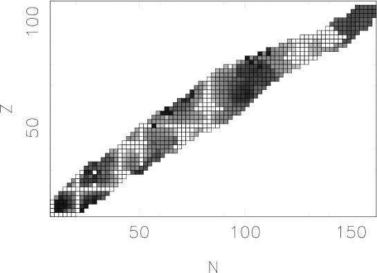
Figure 5: Groundstate quadrupole deformation $|\beta_{2}|$ in our model using the $\chi_{m}$ parameters in a 2-dimensional calculation assuming axially symmetry. White squares denote spherical shapes, the darkest shade of gray represents deformations with $|\beta_{2}|>0.4$.

There are a number of areas where shape isomers exist. Especially in the $Z\sim 70$ range and large neutron number the calculated energies of the oblate and prolate minima are often within a few hundred keV, and, given the approximations involved in this calculation, the true groundstate deformation cannot really be determined (in a more realistic calculation using configuration mixing both minima will mix). It is possible that both states are connected via $\gamma$ deformation. In future 3-dimensional calculations this point should be studied more closely. As an example the Fig. 6 shows the resulting deformation dependence of the energy of very neutron-rich Dysprosium and Erbium isotopes. You see quite deformed prolate and oblate minima with $\beta_{2}\sim 0.45$ and $-0.28$, respectively, that are essentially degenerate. In principle, there are two values for the deformation to be displayed in Fig. 5.

Figure 6: Binding energies of Dy and Er isotopes, relative to the spherical state, as function of deformation. Two nearly degenerate minima can be observed. The horizontal lines show experimental (or extrapolated) values for the binding energy audi

In a comparison with recent experimental results of the deformation of various sulfur and argon isotopes sulfur we calculated the groundstate deformation of ^38-46S and ^42,44Ar. The results can be seen in Figure 7. The experiments determine the absolute value for $\beta_{2}$, the calculations show prolate groundstates for sulfur and oblate ones for argon. Our numbers agree quite well with experiment, some predictions for the sofar undetermined deformation of very neutron rich sulfur isotopes are shown, too.

Figure 7: Quadrupole deformation $|\beta_{2}|$ for sulfur (circles) and argon (squares) isotopes with mass number A. The full symbols denote the theoretical results, the open symbols are experimental data sulfur .

Going to proton-rich side we compare our results of a calculation of axially deformed N=Z nucleus ⁶⁸Se with relatively recent experimental data that show a strongly oblate groundstate ($\beta_{2}\sim-0.3$) together with an excited prolate state Fischer . The result of a quadrupole-constrained calculation is shown in Fig. 8. In accordance with the experiments distinct strongly deformed oblate and prolate minima are found, where the oblate state is more strongly bound by about 2 MeV.

Figure 8: Binding energy of the nucleus ⁶⁸Se (relative to the spherical solution) as function of the quadrupole constraint $\beta_{2}$.

As a further test of calculations of deformed nuclei we look at Nobelium isotopes. The calculation of the deformation of ²⁵²No, ²⁵⁴No, and ²⁵⁶No are shown in Figure 9. The behavior of the different isotopes is very similar, showing a prolate minimum at around $\beta_{2}\sim 0.29$. This compares very well with measurements No of the groundstate deformation of ²⁵²No and ²⁵⁴No with resulting numbers of $\beta_{2}=0.31\pm 0.02$ for A=252 and $\beta_{2}=0.32\pm 0.02$ for A = 254, respectively.

Figure 9: Binding energies of different Nobelium isotopes as function of the quadrupole constraint $\beta_{2}$. The horizontal lines indicate the measured groundstate energy

Finally, we investigated various superdeformed heavy nuclei. In all cases where a superdeformed state is known we could either see a distinct superdeformed minimum or a shoulder indicating the precursor of a superdeformed state for higher spins. As an example Figure 10 shows the result for the mercury isotopes ¹⁹²Hg and ¹⁹⁴Hg, which has originally been predicted to have superdeformed bands in Chas (a study analogous to our discussion using in the RMF approach has be performed in Ring ).

Figure 10: Binding energies of ¹⁹²Hg and ¹⁹⁴Hg as function of $\beta_{2}$. Both isotopes exhibit an oblate groundstate and superdeformed structures for $\beta_{2}\sim 0.7$. Experimental binding energies are indicated by horizontal lines.

Table 3: Parameter set $\chi_{m}$, all numbers are quoted for the appropriate powers in MeV. $G_{p}$ and $G_{n}$ are the strengths of the zero-range pairing force for protons and neutrons, respectively.

$g_{N\sigma}$	-10.569	$g_{N\zeta}$	0.467	$g_{N\omega}$	13.3265	$g_{N\rho}$	5.48851
$k_{0}$	2.47584	$k_{1}$	1.35436	$k_{2}$	-4.93719	$k_{3}$	-2.77257
$k_{4}$	-0.233064	$g_{4}$	79.9083	$\epsilon$	0.02134	$\chi_{0}$	409.76956
$G_{p}$	$-4.47\cdot 10^{-5}$	$G_{n}$	$-4.34\cdot 10^{-5}$	$f_{K}$	122

Table 4: Hadron masses (in MeV) for parameter set $\chi_{m}$. In brackets the experimental isospin-averaged values are shown PDG . Note that in the particle data book $\sigma,\zeta,\delta$ correspond to $f_{0}(400-1200)$, $f_{0}(980)$, and $a_{0}(980)$, respectively.

$m_{N}$	939.2	(938.9)	$m_{\Lambda}$	1115.7	(1115.6)	$m_{\Sigma}$	1196.0	(1193.1)	$m_{\Xi}$	1331.3	(1318.1)
$m_{\pi}$	138.6	(138.0)	$m_{K}$	497.3	(495.6)	$m_{\eta}$	574.0	(547.5)	$m_{\eta^{\prime}}$	897.3	(957.8)
$m_{\sigma}$	466.5	(400 - 1200)	$m_{\zeta}$	1024.5	(980)	$m_{\delta}$	973.26	(985)	$m_{\phi}$	1020.0	(1019.4)
$m_{\omega}$	780.6	(782.0)	$m_{\rho}$	761.1	(768.1)	$m_{\chi}$	960.0

In addition to the oblate groundstate we see a rather complex structure of the energy surface and clear evidence for superdeformation in both cases. An experimental measurement and extrapolation to the groundstate of ¹⁹⁴Hg gave an estimate of an excitation energy $E\sim 6.02~{}$MeV Khoo of the superdeformed state with respect to the oblate minimum. In our calculation we get $E=4.3~{}$MeV, which is a little bit low but in reasonable agreement with experiment. In the case of ¹⁹²Hg we obtain $E=3.1~{}$MeV.

IV Conclusions

We investigated a hadronic model based on chirally symmetric interactions within an flavor-SU(3) approach and calculated nuclear properties within this approach. First we introduced a new improved set of model parameters generated by a fit of a set of spherical nuclei. For the first time also the isospin-triplet $\delta$ meson was taken into account, which naturally occurs within the SU(3) scheme in its coupling to the baryons as well as in the nonlinear meson-meson interactions. The quality of the fit is as good as the results of other relativistic mean field models of nuclear structure. We investigated deformed nuclei and found reasonable results for nuclear quadrupole deformations. A number of improvements should be addressed in future calculations. A projection onto good particle numbers as well as, in case of the deformed calculations, a projection onto good angular momentum should be performed. In different regimes of the nuclear landscape shape isomers are found with minima that are very close in their energies. Especially for those cases three-dimensional studies and a calculation including configuration mixing of the various states have to be done. All these points are currently under investigation later .

- (1) B. D. Serot and J. D. Walecka, Phys. Lett. B87, 172 (1979).
- (2) A. R. Bodmer and C. E. Price, Nucl. Phys. A505, 123 (1989).
- (3) P.-G. Reinhard, Rep. Prog. Phys. 52, 439 (1989).
- (4) G. A. Lalazissis, J. König and P. Ring, Phys. Rev. C 55, 540 (1997).
- (5) Ch. Beckmann, P. Papazoglou, D. Zschiesche, S. Schramm, H. Stöcker, and W. Greiner, Phys. Rev. C 65, 024301 (2002)
- (6) P. Papazoglou, D. Zschiesche, S. Schramm, J. Schaffner-Bielich, H. Stöcker, W. Greiner, Phys. Rev. C59 (1998) 411
- (7) P. Papazoglou, D. Zschiesche, S. Schramm, J. Schaffner-Bielich, H. Stöcker, W. Greiner, Phys. Rev. C55 (1997) 1499
- (8) T. Bürvenich, D. G. Madland, J. A. Maruhn, P.-G. Reinhard, Phys. Rev. C 65, 044308 (2002).
- (9) Clemens Rutz, Ph.D. thesis, University of Frankfurt 1998.
- (10) S. Schramm and D. Zschiesche, preprint nucl-th0204075, submitted to Phys. Rev. C.
- (11) G. Audi and A.H. Wapstra, Nucl. Phys. A595, 409 (1995).
- (12) M. Bender, T. Cornelius, G. A. Lalazissis, J. A. Maruhn, W. Nazarewicz, and P.-G. Reinhard, preprint nucl-th/0110057.
- (13) M. Bender, K. Rutz, P.-G. Reinhard, J. A. Maruhn, and W. Greiner, Eur. Phys. J. A 8,59 (2000).
- (14) G. A. Laizissis, A. R. Farhan, and M. M. Sharma, Nucl. Phys. A628, 221 (1998).
- (15) M. Bender, K. Rutz, T. Buervenich, P.-G. Reinhard, J. A. Maruhn, W. Greiner Proc. Nuclear Structure 98, C. Baktash [ed.], AIP Conf. Proc. 481, AIP, p. 81 (1999).
- (16) T. Buervenich, Ph. D. Thesis, Frankfurt (2002).
- (17) R. Rodriguez-Guzman, J. L. Egido, and L. M. Robledo, preprint nucl-th/0204074 (2002).
- (18) T. Motobayashi et al., Phys. Lett. B346, 9 (1995).
- (19) P. Moller, J. R. Nix, W. D. Myers, and W. J. Swiatecki, Atomic Data Nucl. Data Tables 59, 185-381 (1995)
- (20) H. Schein, T. Glasmacher, B. A. Brown, J. A. Brown, P. D. Cottle, P. G. Hansen, R. Harkewicz, M. Hellström, R. W. Ibbotson, J. K. Jewell, K. W. Kember, D. J. Morrissey, M. Steiner, P. Thirolf, and M. Thoennessen, Phys. Rev. C 77, 3967 (996).
- (21) S. M. Fischer, D. P. Balamuth, P. A. Hausladen, C. J. Lister, M. P. Carpenter, D. Seweryniak, and J. Schwartz, Phys. Rev. Lett. 84, 4064 (2000).
- (22) R.-D. Herzberg et al., Phys. Rev. C 65 014303 (2001).
- (23) R. R. Chasman, Phys. Lett. B219, 227 (1989).
- (24) G. A. Lalazissis and P. Ring, Phys. Lett. B 427, 225 (1998).
- (25) D. E. Groom et al., Eur. Phys. J. C15, 1 (2000).
- (26) T. L. Khoo et al., Phys. Rev. Lett. 76, 1583 (1996).
- (27) S. Schramm, in preparation.