An Alternative Parameterization of ${\bm{R}}$-matrix Theory

Abstract

An alternative parameterization of ${\bm{R}}$-matrix theory is presented which is mathematically equivalent to the standard approach, but possesses features which simplify the fitting of experimental data. In particular there are no level shifts and no boundary-condition constants which allows the positions and partial widths of an arbitrary number of levels to be easily fixed in an analysis. These alternative parameters can be converted to standard ${\bm{R}}$-matrix parameters by a straightforward matrix diagonalization procedure. In addition it is possible to express the collision matrix directly in terms of the alternative parameters.

I Introduction

The ${\bm{R}}$-matrix theory of reactions has proven over the course of time to be very useful in nuclear and atomic physics, both for the fitting of experimental data and as a tool for theoretical calculations. In this paper we explore a mathematically-equivalent alternative formulation of ${\bm{R}}$-matrix theory which will be especially useful for the fitting of experimental nuclear physics data.

In a recent paper an alternative parameterization ${\bm{R}}$-matrix theory was described by Angulo and Descouvemont Ang00 . In their framework there are no level shifts and it is straightforward to incorporate known information about level energies and partial widths. They presented an approximate iterative relation between the alternative parameters and the standard ${\bm{R}}$-matrix parameters. In addition consideration was limited to the single-channel case with a boundary condition constant of zero. Some aspects of these alternative parameters have also been discussed in a paper by Barker Bar71 . In this paper we further develop the concept of an alternative ${\bm{R}}$-matrix parameterization. The description is generalized to allow non-zero boundary condition constants and an arbitrary number of channels. We present an exact method for converting the alternative parameters to the standard ${\bm{R}}$-matrix parameters which only requires a matrix diagonalization. We also found a rather surprising result, that the collision matrix can be calculated directly from the alternative parameters using alternative formulations of the level matrix or ${\bm{R}}$ matrix. We then discuss the solution of the nonlinear eigenvalue equation required to extract the alternative parameters from the standard parameterization, and demonstrate some of these ideas using a simple example. Finally we briefly discuss the application of the alternative parameterization to $\gamma$ rays and $\beta$ decays.

II Review of standard ${\bm{R}}$-Matrix theory

We begin by reviewing some of the notation and results of standard ${\bm{R}}$-matrix theory as described by Lane and Thomas (LT) Lan58 . The ${\bm{R}}$ matrix is a function of the energy $E$ and is defined by

$$R_{c^{\prime}c}=\sum_{\lambda}\frac{\gamma_{\lambda c^{\prime}}\gamma_{\lambda c}}{E_{\lambda}-E},$$ (1)

where $E_{\lambda}$ are the level energies, $\gamma_{\lambda c}$ are the reduced width amplitudes, $\lambda$ is the level label, and $c$ is the channel label. We will assume that the numbers of levels and channels are finite and given by $N_{\lambda}$ and $N_{c}$, respectively. One must also specify the constants $B_{c}$, which determine the boundary conditions satisfied by the underlying eigenfunctions.

In order to calculate physical observables one must employ various combinations of the Coulomb wavefunctions, evaluated at the channel radius $r_{c}=a_{c}$. The quantities $I_{c}$ and $O_{c}$ are defined by (LT, Eq. II.2.13). For closed channels the outgoing solution $O_{c}$ is taken to be the exponentially-decaying Whittaker function (LT, Eq. II.2.17). In addition one defines $\Omega_{c}=(I_{c}/O_{c})^{1/2}$ and

$$L_{c}=\left(\frac{a_{c}}{O_{c}}\frac{\partial O_{c}}{\partial r_{c}}\right)_{a_{c}}=S_{c}+{\rm i}P_{c}$$ (2)

where the shift factor $S_{c}$ and penetration factor $P_{c}$ are real quantities. The collision matrix ${\bm{U}}$ is an $N_{c}\times N_{c}$ matrix which determines the observable quantities; it is related to the ${\bm{R}}$ matrix via (LT, Eq. VII.1):

$${\bm{U}}=2{\rm i}{\bm{\rho}}^{1/2}{\bm{O}}^{-1}[{\bm{1}}-{\bm{R}}({\bm{L}}-{\bm{B}})]^{-1}{\bm{R}}{\bm{\rho}}^{1/2}{\bm{O}}^{-1}+{\bm{I}}{\bm{O}}^{-1}$$ (3)

where ${\bm{O}}$, ${\bm{I}}$, ${\bm{L}}$, ${\bm{B}}$, and ${\bm{\rho}}$ are purely diagonal with elements $O_{c}$, $I_{c}$, $L_{c}$, $B_{c}$, and $k_{c}a_{c}$, respectively; ${\bm{1}}$ is the unit matrix, and $k_{c}$ is the wavenumber.

It is convenient to form the level-space column vector ${\bm{\gamma}}_{c}$ from the $\gamma_{\lambda c}$, and to then form the rectangular matrix ${\bm{\gamma}}$ from the ${\bm{\gamma}}_{c}$ such that the matrix ${\bm{\gamma}}$ has $N_{\lambda}$ rows and $N_{c}$ columns. In addition, the diagonal matrix ${\bm{e}}$ is defined by

$$e_{\lambda\mu}=E_{\lambda}\delta_{\lambda\mu}.$$ (4)

The ${\bm{R}}$ matrix defined by Eq. (1) can now be written succinctly as

$${\bm{R}}={\bm{\gamma}}^{T}({\bm{e}}-E{\bm{1}})^{-1}{\bm{\gamma}}.$$ (5)

The collision matrix can also be expressed as

$${\bm{U}}=2{\rm i}{\bm{\rho}}^{1/2}{\bm{O}}^{-1}{\bm{\gamma}}^{T}{\bm{A}}{\bm{\gamma}}{\bm{\rho}}^{1/2}{\bm{O}}^{-1}+{\bm{I}}{\bm{O}}^{-1},$$ (6)

where ${\bm{A}}$ is an $N_{\lambda}\times N_{\lambda}$ matrix defined by its inverse:

$${\bm{A}}^{-1}={\bm{e}}-E{\bm{1}}-{\bm{\gamma}}({\bm{L}}-{\bm{B}}){\bm{\gamma}}^{T}.$$ (7)

The equivalence of these two forms for the collision matrix is discussed in (LT, Sec. IX.1) and in the Appendix. In addition the elements of the collision matrix connecting open channels in Eq. (6) can also be expressed as

$$U_{c^{\prime}c}=\Omega_{c^{\prime}}\Omega_{c}\left[\delta_{c^{\prime}c}+2{\rm i}(P_{c^{\prime}}P_{c})^{1/2}{\bm{\gamma}}_{c^{\prime}}^{T}{\bm{A}}{\bm{\gamma}}_{c}\right],$$ (8)

using the definitions of the Coulomb functions.

An interesting feature of ${\bm{R}}$-matrix theory is that the collision matrix is invariant under changes in the $B_{c}$, provided that the $E_{\lambda}$ and $\gamma_{\lambda c}$ are suitably adjusted. This result remains true even for the case of finite $N_{\lambda}$ Bar72 . The transformation is most easily described using matrix equations in level space. Let us consider the transformation $B_{c}\rightarrow B_{c}^{\prime}$, $E_{\lambda}\rightarrow E_{\lambda}^{\prime}$, and $\gamma_{\lambda c}\rightarrow\gamma_{\lambda c}^{\prime}$. One first constructs the real and symmetric matrix ${\bm{C}}$ defined by

$${\bm{C}}={\bm{e}}-\sum_{c}{\bm{\gamma}}_{c}{\bm{\gamma}}_{c}^{T}(B_{c}^{\prime}-B_{c}),$$ (9)

which is diagonalized by the orthogonal matrix ${\bm{K}}$ such that ${\bm{D}}={\bm{K}}{\bm{C}}{\bm{K}}^{T}$, with $D_{\lambda\mu}=D_{\lambda}\delta_{\lambda\mu}$. The necessary transformation of the ${\bm{R}}$-matrix parameters is then given by Bar72

$$E_{\lambda}^{\prime}=D_{\lambda}$$ (10)

and

$${\bm{\gamma}}_{c}^{\prime}={\bm{K}}{\bm{\gamma}}_{c}.$$ (11)

It is straightforward to verify by substitution into Eqs. (6,7) that these transformations leave ${\bm{U}}$ invariant.

III The Alternative Parameterization

III.1 Definition of the parameterization

We begin by defining the real and symmetric matrix ${\bm{\mathcal{E}}}$:

$${\bm{\mathcal{E}}}={\bm{e}}-\sum_{c}{\bm{\gamma}}_{c}{\bm{\gamma}}_{c}^{T}(S_{c}-B_{c}),$$ (12)

and consider the eigenvalue equation

$${\bm{\mathcal{E}}}{\bm{a}}_{i}=\tilde{E}_{i}{\bm{a}}_{i}$$ (13)

where $\tilde{E}_{i}$ is the eigenvalue and ${\bm{a}}_{i}$ is the corresponding eigenvector. Note that ${\bm{\mathcal{E}}}$ is implicitly dependent upon $\tilde{E}_{i}$ through $S_{c}$, so the eigenvalue problem is nonlinear. We will assume for convenience that the eigenvectors are normalized so that ${\bm{a}}_{i}^{T}{\bm{a}}_{i}=1$.

Before proceeding further we would like to point out two important properties of this eigenvalue equation: (1) The eigenvalues $\tilde{E}_{i}$ are invariant if the $B_{c}$ are changed and the $E_{\lambda}$ and $\gamma_{\lambda c}$ are changed according to Eqs. (10,11). This result is easily shown by substituting Eqs. (9-11) into Eqs. (12,13). (2) If $B_{c}=S_{c}(E_{\lambda})$, the matrix ${\bm{\mathcal{E}}}$ is diagonal for the energy $E_{\lambda}$ and hence $E_{\lambda}$ is an eigenvalue. For this choice of $B_{c}$ the ${\bm{R}}$-matrix level energy $E_{\lambda}$ is often taken to be the “observed resonance energy”. This definition is particularly useful in the present context and we will thus adopt the $\tilde{E}_{i}$ as the observed resonance energies. The $\tilde{E}_{i}$ also correspond exactly to the level energies found using boundary-condition constant transformations yielding $B_{c}=S_{c}(E_{\lambda})$ such as described by Barker Bar71 and Azuma et al. Azu94 .

In addition one can define a new set of reduced width parameters $\tilde{\gamma}_{ic}$ via

$$\tilde{\gamma}_{ic}={\bm{a}}_{i}^{T}{\bm{\gamma}}_{c}.$$ (14)

These new reduced width parameters are also invariant under changes in $B_{c}$. When $B_{c}=S_{c}(E_{\lambda})$ we have also $\tilde{\gamma}_{\lambda c}=\gamma_{\lambda c}$. The quantities $\tilde{E}_{i}$ and $\tilde{\gamma}_{ic}$ can be taken as an alternative parameterization of ${\bm{R}}$-matrix theory. We will derive below efficient methods to convert $\tilde{E}_{i}$ and $\tilde{\gamma}_{ic}$ into the standard ${\bm{R}}$-matrix parameters $E_{\lambda}$ and $\gamma_{\lambda c}$, or to the collision matrix ${\bm{U}}$. Also note that $\tilde{E}_{i}$ and $\tilde{\gamma}_{ic}$ are equivalent to the “superscript $(\lambda)$” parameters of Barker Bar71 , and essentially equivalent to the “observed” ${\bm{R}}$-matrix parameters described by Angulo and Descouvemont Ang00 .

Our Eq. (13) is closely related to the complex eigenvalue equation introduced by Hale, Brown, and Jarmie Hal87 to locate the poles of the collision matrix – in fact it is just the real part of their eigenvalue equation. For bound states our $\tilde{E}_{i}$ are thus equivalent to the eigenvalues discussed in Ref. Hal87 since $P_{c}=0$. For these states we can also introduce the asymptotic normalization constant $C_{ic}$ which is given by Muk99

$$C_{ic}^{2}=\frac{2\mu_{c}a_{c}}{\hbar^{2}O_{c}^{2}}\left[\frac{\tilde{\gamma}_{ic}^{2}}{1+\sum_{c}\tilde{\gamma}_{ic}^{2}\left(\frac{dS_{c}}{dE}\right)_{\tilde{E}_{i}}}\right],$$ (15)

where $\mu_{c}$ is the reduced mass. This quantity is simply related to the pole residues described by Eq. (4) of Ref. Hal87 . For unbound states there appears to be no simple relation between $\tilde{E}_{\lambda}$ and $\tilde{\gamma}_{\lambda c}$ and the pole parameters of Ref. Hal87 . One may however define the observed partial width of a level in terms of our parameters by

$$\Gamma_{ic}=\frac{2P_{c}\tilde{\gamma}_{ic}^{2}}{1+\sum_{c}\tilde{\gamma}_{ic}^{2}\left(\frac{dS_{c}}{dE}\right)_{\tilde{E}_{i}}}$$ (16)

see (LT, Eqs. XII.3.5 and XII.3.6). One should bear in mind however that there are many different definitions of observed resonance energies and widths in use; generally the differences between definitions are significant only for broad states.

III.2 Relation to standard parameters

We will next show the method to convert $\tilde{E}_{\lambda}$ and $\tilde{\gamma}_{\lambda c}$ to standard ${\bm{R}}$-matrix parameters. It is assumed that the eigenvalues are distinct, so that $\tilde{E}_{i}\neq\tilde{E}_{j}$ provided $i\neq j$. Note that if this were not the case the levels with the same $\tilde{E}_{i}$ could be combined into a single level. The eigenvectors of Eq. (13) are not orthogonal; using the eigenvalue equation with two different eigenvalues one finds

$${\bm{a}}_{j}^{T}({\bm{\mathcal{E}}}_{j}-{\bm{\mathcal{E}}}_{i}){\bm{a}}_{i}=(\tilde{E}_{j}-\tilde{E}_{i}){\bm{a}}_{j}^{T}{\bm{a}}_{i},$$ (17)

where ${\bm{\mathcal{E}}}_{i}$ is used to denote the matrix ${\bm{\mathcal{E}}}$ evaluated for the energy $\tilde{E}_{i}$. Using Eqs. (12,14) with this result we obtain

$${\bm{a}}_{j}^{T}{\bm{a}}_{i}=-\sum_{c}\tilde{\gamma}_{ic}\tilde{\gamma}_{jc}\frac{S_{ic}-S_{jc}}{\tilde{E}_{i}-\tilde{E}_{j}},$$ (18)

where $S_{ic}$ denotes the shift function $S_{c}$ evaluated at $\tilde{E}_{i}$. By similarly evaluating ${\bm{a}}_{j}^{T}({\bm{\mathcal{E}}}_{j}+{\bm{\mathcal{E}}}_{i}){\bm{a}}_{i}$, one finds that

$${\bm{a}}_{j}^{T}{\bm{e}}{\bm{a}}_{i} = \frac{\tilde{E}_{i}+\tilde{E}_{j}}{2}{\bm{a}}_{j}^{T}{\bm{a}}_{i}$$

$$+\sum_{c}\tilde{\gamma}_{ic}\tilde{\gamma}_{jc}\left(\frac{S_{ic}+S_{jc}}{2}-B_{c}\right).$$

These results are summarized in the matrices ${\bm{M}}$ and ${\bm{N}}$:

$${\bm{a}}_{j}^{T}{\bm{a}}_{i}\equiv M_{ij}=\left\{\begin{array}[]{ll}1&i=j\\ -\sum_{c}\tilde{\gamma}_{ic}\tilde{\gamma}_{jc}\frac{S_{ic}-S_{jc}}{\tilde{E}_{i}-\tilde{E}_{j}}&i\neq j\end{array}\right.$$ (20)

and

$${\bm{a}}_{j}^{T}{\bm{e}}{\bm{a}}_{i} \equiv N_{ij}$$ (21)

$$= \left\{\begin{array}[]{ll}\tilde{E}_{i}+\sum_{c}\tilde{\gamma}_{ic}^{2}(S_{ic}-B_{c})&i=j\\ \sum_{c}\tilde{\gamma}_{ic}\tilde{\gamma}_{jc}\left(\frac{\tilde{E}_{i}S_{jc}-\tilde{E}_{j}S_{ic}}{\tilde{E}_{i}-\tilde{E}_{j}}-B_{c}\right)&i\neq j\end{array}\right..$$ (24)

Note that the construction of ${\bm{N}}$ requires the adoption of specific $B_{c}$ values.

The eigenvectors of Eq. (13) can be arranged into a square matrix ${\bm{a}}$ such that Eq. (14) becomes

$$\tilde{\bm{\gamma}}_{c}={\bm{a}}^{T}{\bm{\gamma}}_{c}.$$ (25)

The matrices ${\bm{M}}$ and ${\bm{N}}$ defined above can then be written as ${\bm{M}}={\bm{a}}^{T}{\bm{a}}$ and ${\bm{N}}={\bm{a}}^{T}{\bm{e}}{\bm{a}}$. From Eq. (4) the matrix ${\bm{e}}$ trivially satisfies the eigenvalue equation

$${\bm{e}}{\bm{u}}_{\lambda}=E_{\lambda}{\bm{u}}_{\lambda}.$$ (26)

Upon substitution of ${\bm{u}}_{\lambda}={\bm{a}}{\bm{b}}_{\lambda}$ and multiplying from the left by ${\bm{a}}^{T}$ this equation becomes

$${\bm{N}}{\bm{b}}_{\lambda}=E_{\lambda}{\bm{M}}{\bm{b}}_{\lambda}.$$ (27)

This eigenvalue equation holds the key for transforming from the $\tilde{E}_{i}$-$\tilde{\gamma}_{ic}$ representation to the standard ${\bm{R}}$-matrix parameters $E_{\lambda}$ and $\gamma_{\lambda c}$. The real, symmetric, and energy-independent matrices ${\bm{M}}$ and ${\bm{N}}$ are completely determined by $\tilde{E}_{i}$, $\tilde{\gamma}_{ic}$, and $B_{c}$ using Eqs. (20,21). The $E_{\lambda}$ can thus be determined by finding the eigenvalues of a generalized eigenvalue equation. If the matrix ${\bm{M}}$ is also positive definite then Eq. (27) is known as the symmetric-definite eigenvalue problem and has $N_{\lambda}$ real eigenvalues (see Sec. 8.7 of Ref. Gol96 ). The off-diagonal elements of ${\bm{M}}$ are $\approx-\sum_{c}\tilde{\gamma}_{ic}\tilde{\gamma}_{jc}\frac{dS_{c}}{dE}$ which is typically small compared to unity; ${\bm{M}}$ will be positive definite provided the $\tilde{\gamma}_{ic}$ are not too large and the energy dependences of $S_{c}$ are not too great. Further if ${\bm{M}}$ is not positive definite, the eigenvectors ${\bm{a}}_{i}$ are not real and the transformation to standard ${\bm{R}}$-matrix parameters is not defined. We thus conclude that for physically reasonable $\tilde{\gamma}_{ic}$, $\tilde{E}_{i}$, and $S_{ic}$ the matrix ${\bm{M}}$ will be positive definite; in practice we have found this condition to be easily fulfilled. Finally note that ${\bm{M}}$ is automatically positive definite for any given set of standard parameters since ${\bm{M}}={\bm{a}}^{T}{\bm{a}}$.

The eigenvectors of Eq. (27) ${\bm{b}}_{\lambda}$ can be arranged into a square matrix ${\bm{b}}$ which satisfies the relations

$${\bm{b}}^{T}{\bm{M}}{\bm{b}}={\bm{1}}$$ (28)

and

$${\bm{b}}^{T}{\bm{N}}{\bm{b}}={\bm{e}}.$$ (29)

We therefore have ${\bm{b}}={\bm{a}}^{-1}$ and from Eq. (25) the standard ${\bm{R}}$-matrix reduced widths are given by

$${\bm{\gamma}}_{c}={\bm{b}}^{T}\tilde{\bm{\gamma}}_{c}.$$ (30)

The simultaneous diagonalization of ${\bm{M}}$ and ${\bm{N}}$ thus provides all of the standard ${\bm{R}}$-matrix parameters. Note that any $B_{c}$ can be chosen; the collision matrix ${\bm{U}}$ will be invariant provided the same $B_{c}$ are used in Eqs. (21) and (3) or (7). The numerical solution of Eq. (27) is discussed in Sec. 8.7.2 of Ref. Gol96 ; we have have utilized the LAPACK lapack routine dsygv.

IV Further Development

It is fruitful to investigate alternative forms for the level matrix and the ${\bm{R}}$ matrix which allow the collision matrix to be calculated directly from the alternative parameters.

IV.1 The Alternative Level Matrix

We define the alternative level matrix $\tilde{\bm{A}}$ implicitly via

$${\bm{\gamma}}_{c^{\prime}}^{T}{\bm{A}}{\bm{\gamma}}_{c}\equiv\tilde{\bm{\gamma}}_{c^{\prime}}^{T}\tilde{\bm{A}}\tilde{\bm{\gamma}}_{c}.$$ (31)

In order for this relation to hold, we must have

$${\bm{a}}\tilde{\bm{A}}{\bm{a}}^{T}={\bm{A}},$$ (32)

or equivalently

$$\tilde{\bm{A}}^{-1}={\bm{a}}^{T}{\bm{A}}^{-1}{\bm{a}}$$ (33)

where we have used Eq. (25). We can now substitute Eq. (7) for ${\bm{A}}^{-1}$ and again use Eq. (25) to obtain

$$\tilde{\bm{A}}^{-1} = {\bm{a}}^{T}{\bm{e}}{\bm{a}}-E{\bm{a}}^{T}{\bm{a}}$$

$$-\sum_{c}\tilde{\bm{\gamma}}_{c}\tilde{\bm{\gamma}}_{c}^{T}(S_{c}-B_{c}+{\rm i}P_{c})$$

$$= {\bm{N}}-E{\bm{M}}-\sum_{c}\tilde{\bm{\gamma}}_{c}\tilde{\bm{\gamma}}_{c}^{T}(S_{c}-B_{c}+{\rm i}P_{c}).$$ (35)

The elements of this matrix can now be determined entirely from the alternative parameters with the aid of Eqs. (20,21):

$$(\tilde{\bm{A}}^{-1})_{ij} = (\tilde{E}_{i}-E)\delta_{ij}-\sum_{c}\tilde{\gamma}_{ic}\tilde{\gamma}_{jc}(S_{c}+{\rm i}P_{c})$$ (36)

$$+ \sum_{c}\left\{\begin{array}[]{ll}\tilde{\gamma}_{ic}^{2}S_{ic}&i=j\\ \tilde{\gamma}_{ic}\tilde{\gamma}_{jc}\frac{S_{ic}(E-\tilde{E}_{j})-S_{jc}(E-\tilde{E}_{i})}{\tilde{E}_{i}-\tilde{E}_{j}}&i\neq j\end{array}\right..$$ (39)

Note that the boundary-condition constants $B_{c}$ have now canceled out – a not unexpected result since the alternative parameters and the collision matrix are independent of $B_{c}$. We can now express the collision matrix directly in terms of the alternative parameters using Eqs. (8,31)

$$U_{c^{\prime}c}=\Omega_{c^{\prime}}\Omega_{c}\left[\delta_{c^{\prime}c}+2{\rm i}(P_{c^{\prime}}P_{c})^{1/2}\tilde{\bm{\gamma}}_{c^{\prime}}^{T}\tilde{\bm{A}}\tilde{\bm{\gamma}}_{c}\right].$$ (40)

IV.2 The Alternative ${\bm{R}}$ Matrix

The matrix $\tilde{\bm{R}}$ is an alternative to the standard ${\bm{R}}$ matrix and is defined implicitly via

$$[{\bm{1}}-{\bm{R}}({\bm{L}}-{\bm{B}})]^{-1}{\bm{R}}\equiv({\bm{1}}-{\rm i}\tilde{\bm{R}}{\bm{P}})^{-1}\tilde{\bm{R}},$$ (41)

where ${\bm{P}}$ is a purely diagonal matrix with elements $P_{c}$. By comparison with Eqs. (3,40) we must have

$$({\bm{1}}-{\rm i}\tilde{\bm{R}}{\bm{P}})^{-1}\tilde{\bm{R}}=\tilde{\bm{\gamma}}^{T}\tilde{\bm{A}}\tilde{\bm{\gamma}}.$$ (42)

We proceed by assuming that $\tilde{\bm{R}}$ can be written in the form

$$\tilde{\bm{R}}=\tilde{\bm{\gamma}}^{T}{\bm{Q}}\tilde{\bm{\gamma}}.$$ (43)

In the Appendix we describe a method to derive the level matrix form for the collision matrix [Eq. (6)] from the channel matrix form [Eq. (3)]. This reasoning can also be applied to $\tilde{\bm{R}}$ and $\tilde{\bm{A}}$. We find that in order to satisfy Eq. (42) we must have

$${\bm{Q}}^{-1}=\tilde{\bm{A}}^{-1}+{\rm i}\tilde{\bm{\gamma}}{\bm{P}}\tilde{\bm{\gamma}}^{T}.$$ (44)

A formula for the elements of ${\bm{Q}}^{-1}$ in terms of the alternative parameters can then be found using Eqs. (36,44):

$$(\tilde{\bm{Q}}^{-1})_{ij} = (\tilde{E}_{i}-E)\delta_{ij}-\sum_{c}\tilde{\gamma}_{ic}\tilde{\gamma}_{jc}S_{c}$$ (45)

$$+ \sum_{c}\left\{\begin{array}[]{ll}\tilde{\gamma}_{ic}^{2}S_{ic}&i=j\\ \tilde{\gamma}_{ic}\tilde{\gamma}_{jc}\frac{S_{ic}(E-\tilde{E}_{j})-S_{jc}(E-\tilde{E}_{i})}{\tilde{E}_{i}-\tilde{E}_{j}}&i\neq j\end{array}\right..$$ (48)

Using Eqs. (3,41) the collision matrix can now be written as

$${\bm{U}}=2{\rm i}{\bm{\rho}}^{1/2}{\bm{O}}^{-1}({\bm{1}}-{\rm i}\tilde{\bm{R}}{\bm{P}})^{-1}\tilde{\bm{R}}{\bm{\rho}}^{1/2}{\bm{O}}^{-1}+{\bm{I}}{\bm{O}}^{-1}.$$ (49)

With the $\tilde{\bm{R}}$ matrix defined by Eqs. (43,45) this equation also gives ${\bm{U}}$ in terms of the alternative parameters without reference to the boundary condition constants.

IV.3 Relative merits of $\tilde{\bm{R}}$ and $\tilde{\bm{A}}$

The $\tilde{\bm{R}}$ matrix is more complicated than ${\bm{R}}$ and the calculation of ${\bm{U}}$ via Eq. (49) requires inverting a real $N_{\lambda}\times N_{\lambda}$ matrix in addition to a complex $N_{c}\times N_{c}$ matrix. When calculating ${\bm{U}}$ via the alternative level matrix one must invert a single complex $N_{\lambda}\times N_{\lambda}$ matrix – using the alternative ${\bm{R}}$ matrix approach may thus offer a modest computational advantage in comparison when $N_{\lambda}\gg N_{c}$. Note however that if it is necessary to calculate ${\bm{U}}$ for several energies and $N_{\lambda}>N_{c}$ it will probably be more computationally efficient to diagonalize Eq. (27) once and then use the standard ${\bm{R}}$-matrix parameters in Eq. (3) to calculate ${\bm{U}}$, as Eq. (3) only requires inverting a single complex $N_{c}\times N_{c}$ matrix.

We would also like to point out that this alternative parameterization, using $\tilde{E}_{i}$ and $\tilde{\gamma}_{ic}$ with Eq. (40) or (49), may be of formal interest since no arbitrary boundary condition constants are required, but the equations are mathematically equivalent to the standard ${\bm{R}}$-matrix approach. The alternative parameters in fact correspond to eigenfunctions satisfying energy-dependent boundary conditions – the real part of the Kapur-Peierls or Siegert boundary conditions see (LT, Sec. IX.2).

V Solution of the Nonlinear Eigenvalue Equation

Table 1: Standard ${\bm{R}}$-matrix parameters from Table III of Ref. Azu94 which describe $J^{\pi}=1^{-}$ reactions in the ${}^{16}{\rm O}$ system, and the alternative parameters derived from them. The channel labels $\alpha$ and $\gamma$ describe ${}^{12}{\rm C}+\alpha$ and ${}^{16}{\rm O}+\gamma$, respectively. The channel radius is 6.5 fm and the boundary condition constant is chosen so that the level shift vanishes for $E=E_{1}$. The $\beta$-decay feeding amplitudes ${\mathcal{B}}_{\lambda}$ are equivalent to the quantities $A_{\lambda 1}\gamma_{\lambda 1}^{-1}N_{\alpha}^{-1/2}$ of Ref. Azu94 .

$\lambda$	1	2	3
$E_{\lambda}$ (MeV)	$-0.0451$	$2.845$	$11.71$
$\gamma_{\lambda\alpha}$ (MeV1/2)	$0.0793$	$0.330$	$1.017$
$\gamma_{\lambda\gamma}$ (MeV-1)	$8.76\times 10^{-6}$	$-2.44\times 10^{-6}$	$-2.82\times 10^{-6}$
${\mathcal{B}}_{\lambda}$	$1.194$	$0.558$	$-0.629$
$\tilde{E}_{\lambda}$ (MeV)	$-0.0451$	$2.400$	$8.00$
$\tilde{\gamma}_{\lambda\alpha}$ (MeV1/2)	$0.0793$	$0.471$	$0.912$
$\tilde{\gamma}_{\lambda\gamma}$ (MeV-1)	$8.76\times 10^{-6}$	$-3.20\times 10^{-6}$	$-2.50\times 10^{-6}$
$\tilde{\mathcal{B}}_{\lambda}$	$1.194$	$0.408$	$-0.781$

The transformation from $\tilde{E}_{ic}$ and $\tilde{\gamma}_{ic}$ to the standard ${\bm{R}}$-matrix parameters $E_{\lambda}$ and $\gamma_{\lambda c}$ can be carried out in a straightforward manner using the methods discussed above in Subsec. III.2. We will now discuss the inverse transformation, i.e. the solution of the nonlinear eigenvalue problem Eq. (13). At this point it is instructive to introduce a concrete example: in Table 1 we show a simple well-documented set of standard ${\bm{R}}$-matrix parameters taken from Azuma et al. Azu94 .

We consider the linear eigenvalue equation

$${\bm{\mathcal{E}}}(E)\hat{\bm{a}}_{i}=\hat{E}_{i}\hat{\bm{a}}_{i}$$ (50)

where ${\bm{\mathcal{E}}}$, the eigenvalues $\hat{E}_{i}$, and eigenvectors $\hat{\bm{a}}_{i}$ depend upon on the energy parameter $E$. The solutions to the original nonlinear problem Eq. (13) thus occur when $\hat{E}_{i}(E)=E$ in which case $E=\tilde{E}_{i}$. From inspection of Eqs. (9,12) we see that the eigenvalues $\hat{E}_{i}$ also correspond to a set of standard ${\bm{R}}$-matrix level energies, transformed from the original parameter values to $B_{c}=S_{c}(E)$.

We will next investigate how the $\hat{E}_{i}$ depend on $E$. Starting with

$$\hat{E}_{i}=\hat{\bm{a}}_{i}^{T}{\bm{\mathcal{E}}}\hat{\bm{a}}_{i}$$ (51)

differentiation with respect to $E$ yields

$$\frac{d\hat{E}_{i}}{dE} = \hat{\bm{a}}_{i}^{T}\frac{d{\bm{\mathcal{E}}}}{dE}\hat{\bm{a}}_{i}+\frac{d\hat{\bm{a}}_{i}^{T}}{dE}{\bm{\mathcal{E}}}\hat{\bm{a}}_{i}+\hat{\bm{a}}_{i}^{T}{\bm{\mathcal{E}}}\frac{d\hat{\bm{a}}_{i}}{dE}$$ (52)

$$= -\hat{\bm{a}}_{i}^{T}\left(\sum_{c}{\bm{\gamma}}_{c}{\bm{\gamma}_{c}}^{T}\,\frac{dS_{c}}{dE}\right)\hat{\bm{a}}_{i}$$

$$+\hat{E}_{i}\left(\frac{d\hat{\bm{a}}_{i}^{T}}{dE}\hat{\bm{a}}_{i}+\hat{\bm{a}}_{i}^{T}\,\frac{d\hat{\bm{a}}_{i}}{dE}\right).$$

Since by definition $\hat{\bm{a}}_{i}^{T}\hat{\bm{a}}_{i}=1$ we have $\frac{d\hat{\bm{a}}_{i}^{T}}{dE}\hat{\bm{a}}_{i}+\hat{\bm{a}}_{i}^{T}\,\frac{d\hat{\bm{a}}_{i}}{dE}=0$ and we finally find

$$\frac{d\hat{E}_{i}}{dE}=-\sum_{c}({\bm{\gamma}}_{c}^{T}\hat{\bm{a}}_{i})^{2}\frac{dS_{c}}{dE}.$$ (54)

The energy derivative of the shift function $\frac{dS_{c}}{dE}$ is positive for negative-energy channels, and is $\geq 0$ for positive-energy channels for all cases we are aware of. This point is also discussed by (LT, p. 350); although a general proof of $\frac{dS_{c}}{dE}\geq 0$ is lacking it appears to always hold in practice and we will thus assume it is true here. Note that for any specific case it is a simple matter to verify this relation numerically.

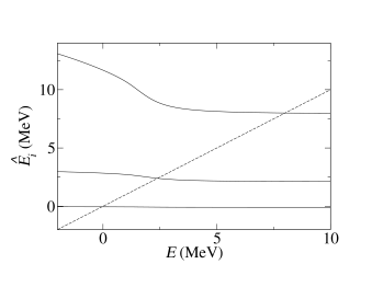
Figure 1: The eigenvalue trajectories are shown by plotting as solid curves the eigenvalues $\hat{E}_{i}$ versus $E$; the dashed line corresponds to $\hat{E}_{i}=E$. The eigenvalues of Eq. (13) are given by the intersections between the solid curves and the dashed line.

Since $({\bm{\gamma}}_{c}^{T}\hat{\bm{a}}_{i})^{2}$ is clearly $\geq 0$, we can utilize $\frac{dS_{c}}{dE}\geq 0$ to conclude from Eq. (54) that

$$\frac{d\hat{E}_{i}}{dE}\leq 0.$$ (55)

The eigenvalues $\hat{E}_{i}$ are thus monotonically non-increasing functions of $E$. The eigenvalue trajectories for the example parameters are shown in Fig. 1 where the expected behavior is seen. We also note the the eigenvalue trajectories avoid crossing one another for the reasons given by von Neumann and Wigner Neu29 . The avoided-crossing behavior is most apparent when there are two nearby levels with very different reduced width amplitudes.

The nonlinear eigenvalue problem Eq. (13) and the parametric eigenvalue problem Eq. (51) are also closely related to a well-studied question in linear algebra: the modification of a symmetric matrix with known eigenvalues and eigenvectors by a positive-definite perturbation. This question is analyzed for the single-channel case in Sec. 8.5.3 of Golub and Van Loan Gol96 and for the multi-channel case by Arbenz, Gander, and Golub Arb88 . The perturbation bounds on the eigenvalues derived in Ref. Arb88 imply that the $\hat{E}_{i}$ remain finite provided the $S_{c}$ are finite – thus the eigenvalue trajectories do not have real poles for $|E|<\infty$.

From the lack of poles and the monotonic dependence $\frac{d\hat{E}_{i}}{dE}\leq 0$ we can conclude that each eigenvalue trajectory intersects with the line $\hat{E}_{i}=E$ exactly once. These intersections are shown graphically for the example in Fig. 1. We thus have the important result that the non-linear eigenvalue problem Eq. (13) has a number of real eigenvalues exactly equal to the number of ${\bm{R}}$-matrix levels. A similar type of nonlinear eigenvalue problem has been investigated by Rogers Rog64 ; it may be that the methods described in that paper could be used to develop further understanding of the present problem, e.g. to investigate inner products and/or the linear independence of the eigenvectors.

The eigenvalues of Eq. (13) satisfy the characteristic equation

$${\rm det}({\bm{\mathcal{E}}}-E{\bm{1}})=0$$ (56)

which can also be written as

$${\rm det}\left[{\bm{e}}-E{\bm{1}}-{\bm{\gamma}}({\bm{S}}-{\bm{B}}){\bm{\gamma}}^{T}\right]=0,$$ (57)

where ${\bm{S}}$ is a purely diagonal matrix with elements $S_{c}$ which depend upon $E$. Using the methods described in Ref. Arb88 one can show that

$${\rm det}\left[{\bm{e}}-E{\bm{1}}-{\bm{\gamma}}({\bm{S}}-{\bm{B}}){\bm{\gamma}}^{T}\right]={\rm det}({\bm{e}}-E{\bm{1}})$$

$$\times\,\,{\rm det}\left[{\bm{1}}-{\bm{\gamma}}^{T}({\bm{e}}-E{\bm{1}})^{-1}{\bm{\gamma}}({\bm{S}}-{\bm{B}})\right].$$

The eigenvalues thus satisfy

$${\rm det}({\bm{e}}-E{\bm{1}})\,{\rm det}\left[{\bm{1}}-{\bm{R}}({\bm{S}}-{\bm{B}})\right]=0,$$ (59)

which may be a computationally-efficient approach for determining the eigenvalues when $N_{\lambda}>N_{c}$ since the calculation of ${\rm det}({\bm{e}}-E{\bm{1}})$ is trivial. Note that Eq. (59) is the multi-channel arbitrary-$B_{c}$ generalization of the resonance condition given by Eq. (14) of Ref. Ang00 . The eigenvalues also satisfy

$${\rm det}\left[{\bm{1}}-{\bm{R}}({\bm{S}}-{\bm{B}})\right]=0,$$ (60)

but this equation has poles in addition to zeros, and if there is a level $\lambda$ with $B_{c}=S_{c}(E_{\lambda})$ (at most one level can satisfy this condition) it does not produced a zero.

Table 2: Elements $b_{ij}$ of the transformation matrix ${\bm{b}}$ corresponding to the parameters of Table 1.

	1	2	3
1	$1.000$	$0.0373$	$0.0446$
2	$0.000$	$0.9781$	$0.2281$
3	$0.000$	$-0.1466$	$0.9933$

Rather than finding the eigenvalues by directly solving the characteristic equation, we have applied the Rayleigh Quotient Iteration method described in Sec. 8.2.3 of Ref. Gol96 to Eq. (13), as this procedure yields the eigenvectors as well as eigenvalues. Starting values for the eigenvalues and eigenvectors were taken as $\tilde{E}_{i}=E_{i}+\sum_{c}\gamma_{ic}^{2}[S_{c}(E_{i})-B_{c}]$ and $a_{ji}=\delta_{ji}$. Due to the nonlinear nature of the problem, the matrix ${\bm{\mathcal{E}}}$ must be updated at each step of the iteration. These procedures were tested with several single-channel and multi-channel parameter sets, and were successful in finding all of the eigenvalues in every case. We cannot rule out however that some cases may require more carefully chosen starting values. Once the $\tilde{E}_{i}$ and ${\bm{a}}_{i}$ are found, the $\tilde{\gamma}_{ic}$ can be calculated using Eq. (14). In Table 1 we show for the example case the alternative parameters determined from the standard ${\bm{R}}$-matrix parameters. Note that the alternative parameters are exactly the same as the ${\bm{R}}$-matrix parameters given in the last column of Table III of Ref. Azu94 which have been transformed to satisfy $B_{c}=S_{c}(E_{\lambda})$ for other levels. As discussed in Subsec. III.1 this equality is required due to our definition of the alternative parameters. In Table 2 we show the elements of the matrix ${\bm{b}}$ for the example parameters. Finally we would like to point out that the methods discussed in this section should be generally useful for the extraction of resonance parameters from standard ${\bm{R}}$-matrix parameters.

VI Application to ${\bm{\gamma}}$ Rays and ${\bm{\beta}}$ Decays

We will briefly discuss the application of the alternative parameterization to reactions involving $\gamma$ rays and $\beta$ decays. Gamma-ray decay processes are generally treated with first-order perturbation theory in ${\bm{R}}$-matrix theory, which implies that $\gamma$-ray channels are excluded from the sum over channels when constructing ${\bm{A}}$, $\tilde{\bm{A}}$, ${\bm{M}}$, or ${\bm{N}}$. Assuming that external contributions can be ignored, the collision matrix elements connecting $\gamma$-ray channels (labeled $\gamma$) and non-$\gamma$-ray channels (labeled $c$) are given by (LT, Eq. XIII.3.9)

$$U_{c\gamma} = 2{\rm i}\Omega_{c}(P_{c}P_{\gamma})^{1/2}\sum_{\lambda\mu}\gamma_{\lambda c}\gamma_{\mu\gamma}A_{\lambda\mu}$$

$$= 2{\rm i}\Omega_{c}(P_{c}P_{\gamma})^{1/2}{\bm{\gamma}}_{c}^{T}{\bm{A}}{\bm{\gamma}}_{\gamma}.$$

In the long-wavelength approximation the penetration factor for $\gamma$ rays is given by $P_{\gamma}=E_{\gamma}^{2\ell+1}$ where $\ell$ is the multipolarity. The observed $\gamma$-ray widths are described by Eq. (16), where $\gamma$-ray channels are excluded from the sum in the denominator. Using the same reasoning described in Subsec. IV.1 the alternative expression for the collision matrix elements can be obtained using the replacement

$${\bm{\gamma}}_{c}^{T}{\bm{A}}{\bm{\gamma}}_{\gamma}=\tilde{\bm{\gamma}}_{c}^{T}\tilde{\bm{A}}\tilde{\bm{\gamma}}_{\gamma},$$ (62)

where the alternative $\gamma$-ray reduced width amplitudes are related to the standard parameters via

$${\bm{\gamma}}_{\gamma}={\bm{b}}^{T}\tilde{\bm{\gamma}}_{\gamma}.$$ (63)

If the external contributions to the matrix elements are included using the formalism of Barker and Kajino Bar91 , the expressions for the collision matrix elements and observed widths become more complicated. However these quantities can still be written in terms of the alternative parameters using the above equations, noting that the $\gamma_{\lambda\gamma}$ above are the internal $\gamma$-ray reduced width amplitudes.

The extension of the alternative parameterization to the description of $\beta$-delayed particle spectra is straightforward. A multi-channel formula for the particle spectrum is given by Eq. (7) of Barker and Warburton Bar88 ; note that additional parameters must now be introduced, the $\beta$-decay feeding amplitudes ${\mathcal{B}}_{\lambda x}$. It is convenient to form column vectors ${\bm{\mathcal{B}}}_{x}$ from the ${\mathcal{B}}_{\lambda x}$, so that $\sum_{\lambda\mu}{\mathcal{B}}_{\lambda x}A_{\lambda\mu}\gamma_{\mu c}$ can be written as ${\bm{\gamma}}_{c}^{T}{\bm{A}}{\bm{\mathcal{B}}}_{x}$. Again using the reasoning of Subsec. IV.1 we have

$${\bm{\gamma}}_{c}^{T}{\bm{A}}{\bm{\mathcal{B}}}_{x}=\tilde{\bm{\gamma}}_{c}^{T}\tilde{\bm{A}}\tilde{\bm{\mathcal{B}}}_{x},$$ (64)

where the alternative feeding amplitudes $\tilde{\bm{\mathcal{B}}}_{x}$ are related to the standard parameters via

$${\bm{\mathcal{B}}}_{x}={\bm{b}}^{T}\tilde{\bm{\mathcal{B}}}_{x}.$$ (65)

Note also that if $B_{c}=S_{c}(E_{\lambda})$ we have $\tilde{\mathcal{B}}_{\lambda x}={\mathcal{B}}_{\lambda x}$. The $\beta$-delayed particle spectrum can now be calculated directly from the alternative parameters by using Eq. (64) in Eq. (7) of Ref. Bar88 . One could also convert to standard ${\bm{R}}$-matrix parameters using Eq. (65) and the methods discussed in Subsec. III.2, and then calculate the spectrum using standard ${\bm{R}}$-matrix formulas.

In Table 1 we also show the standard and alternative $\gamma$-ray reduced amplitudes and $\beta$-decay feeding amplitudes for the example case.

VII Conclusions

We have presented an alternative formulation of ${\bm{R}}$-matrix theory based on the parameters $\tilde{E}_{i}$ and $\tilde{\gamma}_{ic}$ defined in Subsec. III.1. This parameterization is a generalization of the ideas presented by Angulo and Descouvemont Ang00 . The new formulation is mathematically equivalent to the standard ${\bm{R}}$-matrix theory Lan58 but there are no boundary condition constants or level shifts. The new parameters can be converted to standard ${\bm{R}}$-matrix parameters by diagonalizing Eq. (27), or be used to calculate the collision matrix directly using Eqs. (40) or (49). We have discussed the solution of the nonlinear eigenvalue problem Eq. (13) which is needed to convert standard ${\bm{R}}$-matrix parameters to the new parameterization. Finally we have briefly discussed the application to $\gamma$ rays and $\beta$ decays.

We can envision at least two uses for this new formulation in the fitting of experimental data. One application is the generation of starting parameter values from an outside source of spectroscopic information such as a level compilation or shell-model calculation. These latter sources generally do not supply standard ${\bm{R}}$-matrix parameters but rather resonance parameters without level shifts. In the past the methods to incorporate these types of information have not always been optimal (e.g. $B_{c}$ could be chosen to make the level shift vanish for a representative energy, but not for all energies simultaneously). Another application is to use the alternative parameters as the fit parameters. The calculations can be made directly from the alternative parameters using the methods discussed in Sec. IV, or by diagonalizing Eq. (27) to find the standard ${\bm{R}}$-matrix parameters. The latter option may be preferable if $N_{\lambda}>N_{c}$, if observables must be calculated for many different energies. It should be noted that in data-fitting applications the collision matrix must be calculated repeatedly for different energies, and the extra computational overhead required will be negligible in comparison. With the alternative parameters it is very easy to fix known information about level energies and partial widths for any number of levels.

*

Appendix A

The equivalence of the two forms of the collision matrix given by Eqs. (3,6) is discussed in (LT, Sec. IX.1). The derivation is reviewed here, utilizing the matrix notation introduced in Sec. II. The same procedure is useful for the derivation of the alternative ${\bm{R}}$ matrix as discussed in Subsec. IV.2.

We define ${\bm{L}}_{0}={\bm{L}}-{\bm{B}}$ and note the quantity $[{\bm{1}}-{\bm{R}}({\bm{L}}-{\bm{B}})]^{-1}$ in Eq. (3) can be written as

$$({\bm{1}}-{\bm{R}}{\bm{L}}_{0})^{-1}=$$

$$[{\bm{L}}_{0}-({\bm{L}}_{0}{\bm{\gamma}}^{T})({\bm{e}}-E{\bm{1}})^{-1}({\bm{\gamma}}{\bm{L}}_{0})]^{-1}{\bm{L}}_{0}.$$

A useful identity is given by

$$({\bm{X}}+{\bm{Z}}{\bm{Y}}{\bm{Z}}^{T})^{-1}={\bm{X}}^{-1}$$

$$-{\bm{X}}^{-1}{\bm{Z}}({\bm{Y}}^{-1}+{\bm{Z}}^{T}{\bm{X}}^{-1}{\bm{Z}})^{-1}{\bm{Z}}^{T}{\bm{X}}^{-1},$$

which holds for any square and invertible matrices ${\bm{X}}$ and ${\bm{Y}}$ which need not be of the same dimension Zha99 . With the aid of this identity we obtain

$$({\bm{1}}-{\bm{R}}{\bm{L}}_{0})^{-1}=\biggl{\{}{\bm{L}}_{0}^{-1}-{\bm{L}}_{0}^{-1}({\bm{L}}_{0}{\bm{\gamma}}^{T})\times\biggr{.}$$ (70)

$$\left[-({\bm{e}}-E{\bm{1}})+({\bm{\gamma}}{\bm{L}}_{0}){\bm{L}}_{0}^{-1}({\bm{L}}_{0}{\bm{\gamma}}^{T})\right]^{-1}({\bm{\gamma}}{\bm{L}}_{0}){\bm{L}}_{0}^{-1}\biggl{\}}{\bm{L}}_{0}$$

$$\hskip 18.06749pt={\bm{1}}+{\bm{\gamma}}^{T}({\bm{e}}-E{\bm{1}}-{\bm{\gamma}}{\bm{L}}_{0}{\bm{\gamma}}^{T})^{-1}{\bm{\gamma}}{\bm{L}}_{0}$$

$$\hskip 18.06749pt={\bm{1}}+{\bm{\gamma}}^{T}{\bm{A}}{\bm{\gamma}}{\bm{L}}_{0},$$

where in the last step we have used Eq. (7) for the definition of the level matrix ${\bm{A}}$.

We can then write

$$({\bm{1}}-{\bm{R}}{\bm{L}}_{0})^{-1}{\bm{R}} = ({\bm{1}}+{\bm{\gamma}}^{T}{\bm{A}}{\bm{\gamma}}{\bm{L}}_{0})\times\hskip 54.2025pt$$

$${\bm{\gamma}}^{T}({\bm{e}}-E{\bm{1}})^{-1}{\bm{\gamma}}$$

$$= {\bm{\gamma}}^{T}({\bm{e}}-E{\bm{1}})^{-1}{\bm{\gamma}}$$ (72)

$$+{\bm{\gamma}}^{T}{\bm{A}}[-{\bm{A}}^{-1}+({\bm{e}}-E{\bm{1}})]({\bm{e}}-E{\bm{1}})^{-1}{\bm{\gamma}}$$

where we have substituted $-{\bm{A}}^{-1}+({\bm{e}}-E{\bm{1}})$ for ${\bm{\gamma}}{\bm{L}}_{0}{\bm{\gamma}}^{T}$. Simplifying this expression we finally have

$$({\bm{1}}-{\bm{R}}{\bm{L}}_{0})^{-1}{\bm{R}}={\bm{\gamma}}^{T}{\bm{A}}{\bm{\gamma}}$$ (73)

which proves the equivalence of Eqs. (3,6).

References

- (1) C. Angulo and P. Descouvemont, Phys. Rev. C 61, 064611 (2000). We have utilized a notation somewhat different from these authors, in order that we could retain the well-established notation of Lane and Thomas Lan58 . The quantities and of this reference correspond to and in the present work. Note also that Ref. Ang00 only considered the single-channel case.
- (2) F. C. Barker, Aust. J. Phys 24, 777 (1971). The quantities and of this reference correspond to and in the present work.
- (3) A. M. Lane and R. G. Thomas, Rev. Mod. Phys. 30, 257 (1958).
- (4) F. C. Barker, Aust. J. Phys. 25, 341 (1972).
- (5) R. E. Azuma, L. Buchmann, F. C. Barker, C. A. Barnes, J. M. D’Auria, M. Dombsky, U. Giesen, K. P. Jackson, J. D. King, R. G. Korteling, P. McNeely, J. Powell, G. Roy, J. Vincent, T. R. Wang, S. S. M. Wong, and P. R. Wrean, Phys. Rev. C 50, 1194 (1994).
- (6) G. M. Hale, R. E. Brown, and N. Jarmie, Phys. Rev. Lett. 59, 763 (1987).
- (7) A. M. Mukhamedzhanov and R. E. Tribble, Phys. Rev. C 59, 3418 (1999).
- (8) G. H. Golub and C. F. Van Loan, Matrix Computations, 3rd Ed. (Johns Hopkins University Press, Baltimore, 1996).
- (9) E. Anderson Z. Bai, C. Bischof, S. Blackford, J. Demmel, J. Dongarra, J. Du Croz, A. Greenbaum, S. Hammarling, A. McKenney, D. Sorensen, LAPACK Users’ Guide, 3rd Ed. (Society for Industrial and Applied Mathematics, Philadelphia, 1999).
- (10) J. von Neumann and E. Wigner, Phys. Z. 30, 467 (1929); English translation in R. S. Knox and A. Gold, Symmetry in the Solid State (Benjamin, New York, 1964), p. 167.
- (11) P. Arbenz, W. Gander, and G. H. Golub, Linear Algebra Appl. 104, 75 (1988).
- (12) E. H. Rogers, Arch. Ration. Mech. Anal. 19, 89 (1964).
- (13) F. C. Barker and T. Kajino, Aust. J. Phys. 44, 369 (1991).
- (14) F. C. Barker and E. K. Warburton, Nucl. Phys. A487, 269 (1988).
- (15) F. Zhang, Matrix Theory: Basic Results and Techniques (Springer-Verlag, New York, 1999), p. 43.