The Axial -Vector Current in Nuclear Many-Body Physics

Abstract

Weak-interaction currents are studied in a recently proposed effective field theory of the nuclear many-body problem. The Lorentz-invariant effective field theory contains nucleons, pions, isoscalar scalar ($\sigma$) and vector ($\omega$) fields, and isovector vector ($\rho$) fields. The theory exhibits a nonlinear realization of $SU(2)_{L}\times SU(2)_{R}$ chiral symmetry and has three desirable features: it uses the same degrees of freedom to describe the axial-vector current and the strong-interaction dynamics, it satisfies the symmetries of the underlying theory of quantum chromodynamics, and its parameters can be calibrated using strong-interaction phenomena, like hadron scattering or the empirical properties of finite nuclei. Moreover, it has recently been verified that for normal nuclear systems, it is possible to systematically expand the effective lagrangian in powers of the meson fields (and their derivatives) and to reliably truncate the expansion after the first few orders. Here it is shown that the expressions for the axial-vector current, evaluated through the first few orders in the field expansion, satisfy both PCAC and the Goldberger–Treiman relation, and it is verified that the corresponding vector and axial-vector charges satisfy the familiar chiral charge algebra. Explicit results are derived for the Lorentz-covariant, axial-vector, two-nucleon amplitudes, from which axial-vector meson-exchange currents can be deduced.

I Introduction

Although quantum chromodynamics (QCD) is known to be the fundamental theory of the strong interaction, it is much more efficient to use hadronic degrees of freedom to describe few- and many-body nuclear systems at low energies. Considerable effort over the last 30 years has shown that models based on baryons and mesons can provide a realistic description of the nucleon–nucleon (NN) interaction, nuclear matter saturation, and the bulk and single-particle properties of finite nuclei. (For reviews, see, for example, Refs. Mac89 ; Mac00 ; Wal95 ; Ser86 ; Ser97 .) The hadrons are described by effective fields whose interactions are determined by a local, Lorentz-invariant lagrangian. The modern viewpoint Wei79 ; Wei95 is that the resulting relativistic, quantum, effective field theory provides the most general way to parametrize an $S$ matrix (or other observables FHT01 ) that is consistent with the constraints of quantum mechanics, special relativity, unitarity, causality, cluster decomposition, and the desired internal symmetries. Thus there is no reason that relativistic quantum field theory should be reserved for “elementary” particles only. We will refer to Lorentz-covariant, relativistic effective field theories based on hadrons as quantum hadrodynamics or QHD Wal74 ; Ser86 ; Ser97 ; Com00 ; Ser00 .

It has also been known for many years that an accurate description of electroweak interactions in nuclei requires a consideration of mesonic degrees of freedom (i.e., “fields”) in addition to the nucleons. (For a review, see Refs. Dub76 ; Rho79 ; Ris89 . An example of more recent work is Ref. Dmi98 .) The mesons are responsible for the forces between the nucleons and also lead to meson-exchange currents (MEC) that contribute to electroweak processes. A desirable theory of the axial-vector current should satisfy the following three conditions:

• It should use the same degrees of freedom to describe the axial current and the strong-interaction dynamics ($\pi$N scattering, NN scattering, and nuclear structure); the basic phenomenological features of the latter are well known.

• It should satisfy the same internal symmetries as the underlying theory of QCD: the discrete symmetries of the strong interaction and (approximate) isospin and chiral symmetries, with the last being spontaneously broken. The enforcement of the continuous symmetries is necessary to ensure the conservation of the vector, isovector current (CVC) and the partial conservation of the axial-vector, isovector current (PCAC).

• It should be possible to calibrate the parameters of the theory using strong-interaction phenomena, like $\pi$N scattering and the properties of finite nuclei, so that one can deduce well-defined and unambiguous currents to be used in the calculation of electroweak processes. This is especially important in effective field theories, because these contain all (non-redundant) interaction terms that are consistent with the underlying symmetries Wei95 ; Ser97 .

In discussing MEC for the weak interaction, CVC implies that the vector part of the current can be determined by performing an isospin rotation on the isovector part of the electromagnetic current Wal95 . Thus the vector parts of the weak exchange currents can be derived from the isovector part of the corresponding electromagnetic exchange currents, which have been determined accurately over the last two decades. In contrast, the axial-vector parts of the exchange currents require additional theoretical input.

There have been many attempts to describe axial-vector exchange currents (AXC) in models based on hadronic degrees of freedom. An important, early contribution was made by Kubodera, Delorme, and Rho Kub78 , who predicted the dominant long-range piece of the AXC using current algebra and the assumption of pion-exchange dominance, which yield the leading-order terms in an expansion in inverse powers of the nucleon mass. Some interesting recent approaches include: a description of AXC using all the degrees of freedom contained in the phenomenological NN potential Blu92 ; Kir92 ; Kir94 ; Ris94 , a model based on “hard pions” Iva79 ; Tow92 ; Con96 ; Sme97 , and the application of chiral perturbation theory (ChPT) Rho91 ; Par93 ; Par94 ; Par96 .

While these approaches enjoyed several successes Lee93 ; Ris94 , they all contain shortcomings that make them undesirable, at least according to the criteria presented above. In particular, current-algebra techniques are difficult to extend to multi-pion contributions or to mesons other than the pion. Models based on a phenomenological NN potential do not explicitly incorporate chiral symmetry and do not explicitly include AXC that arise from the direct interaction of the exchanged mesons with the axial current. Hard-pion models use a linear realization of the chiral symmetry; thus, inclusion of the $\rho$ meson necessitates the inclusion of its chiral partner, the $a_{1}$, which is known to be relatively unimportant in the NN interaction and in nuclear structure Ser92 . Moreover, the strong, mid-range NN attraction, which arises predominantly from correlated two-pion exchange, and which is crucial for an accurate description of NN phase shifts and nuclear matter properties Mac89 ; Ser97 ; Com00 ; LARGE , is difficult to generate in models with linear chiral symmetry without also generating unrealistic many-nucleon forces Fur96 . In contrast, when the chiral symmetry is realized nonlinearly, the mid-range attraction can be efficiently simulated by introducing an effective, scalar, isoscalar, chiral singlet $\sigma$ meson with a mass of roughly 500 MeV TANG95 ; Fur97 .

Finally, models based on ChPT attempt to explain all of the dynamics using nucleons and pions alone; this makes a description of the NN interaction and of nuclear structure very complicated, since one must generate much of the strong-interaction dynamics using multi-pion loop processes Epe98 ; Epe00 ; Epe02 ; Ent02 ; Ent02a . These shortcomings motivate the search for alternative descriptions of the AXC.

In Ref. Ana98 , a lagrangian-based model that contains $\pi$, $\sigma$, and $\omega$ meson fields was used to construct the AXC. This model incorporates the desirable qualities enumerated earlier: it contains the mesons responsible for the dominant features of the NN interaction, it respects both isospin symmetry and (approximate) spontaneously broken chiral symmetry, and (in principle) its parameters can be calibrated to the properties of nuclei by using the mean-field approximation for the meson fields. Nevertheless, the implementation of the chiral symmetry in this model (which is based on the well-known Sigma model Sch57 ; GML60 ; Wal95 ) turns out to be too restrictive. In particular, it is impossible to satisfy both PCAC and the Goldberger–Treiman relation without destroying the familiar chiral charge algebra. It is also impossible to reproduce the empirical equilibrium point of nuclear matter in the mean-field approximation Ker74 ; Fur96 . Moreover, the linear realization of the chiral symmetry makes it cumbersome to include the $\rho$ meson Ser92 . A viable description of the AXC requires a more general implementation of the chiral symmetry.

In the present work, we derive the axial-vector current using a recently proposed QHD lagrangian Fur97 ; Ser97 that contains nucleons and $\pi$, $\sigma$, $\omega$, and $\rho$ mesons. This lagrangian has a linear realization of the $SU(2)_{V}$ isospin symmetry and a nonlinear realization of the spontaneously broken $SU(2)_{L}\times SU(2)_{R}$ chiral symmetry (when the pion mass is zero). It was shown in Refs. Fur97 ; PARAMS ; Ser00 that by using Georgi’s naive dimensional analysis (NDA) Geo93 and the assumption of naturalness (namely, that all appropriately defined, dimensionless couplings are of order unity), it is possible to truncate the lagrangian at terms involving only a few powers of the meson fields and their derivatives, at least for systems at normal nuclear densities. It was also shown that a mean-field approximation to the lagrangian could be interpreted in terms of density functional theory Dre90 ; Ser97 ; Ser02 , so that calibrating the parameters to observed bulk and single-particle nuclear properties incorporates (approximately) many-body effects that go beyond mean-field theory. Explicit calculations of closed-shell nuclei provided such a calibration and verified the naturalness assumption PARAMS . This approach therefore embodies the three desirable features needed for a description of the axial-vector current in the nuclear many-body problem.

This effective field theory (EFT) also overcomes the difficulties found in Ref. Ana98 . The chiral symmetry guarantees that the PCAC condition will hold for the one- and two-body axial currents and pion-production amplitudes, as we demonstrate explicitly below. Moreover, the $\pi$N coupling strength $g_{A}$ enters as a free parameter that can be chosen so that the Goldberger–Treiman relation is satisfied at the tree level, without any rescaling of the fields. This result, together with the chiral symmetry, ensures that the conserved vector and axial-vector charges obey the familiar algebra. Thus all three required constraints can be satisfied simultaneously in the present framework. Moreover, the pion–pion and pion–nucleon parts of the lagrangian are exactly the same as those of chiral perturbation theory Gas88 ; Ell98 ; Bira .

It is important to note that in our EFT, only the pions and nucleons (the stable particles) can appear on external lines with timelike four-momenta. The heavy non-Goldstone bosons appear only on internal lines (with spacelike four-momenta) and allow us to parametrize the medium- and short-range parts of the nucleon–nucleon interaction, as well as the electromagnetic form factors of the hadrons TANG95 ; Fur97 . The heavy bosons are also convenient degrees of freedom for describing nonvanishing expectation values of bilinear nucleon operators, like ${\overline{N\mkern 3.0mu}\mkern-3.0mu}{}\mkern 2.0muN$ and ${\overline{N\mkern 3.0mu}\mkern-3.0mu}{}\mkern 2.0mu\gamma^{\mu}N$, which are important in nuclear many-body systems Ser86 ; Ser97 .

The remainder of this paper is organized as follows. In Sec. II, the effective QHD lagrangian is introduced and described briefly, and the vector and axial-vector currents are derived for the interaction terms that contain only one derivative of the pion field. The currents arise directly from Noether’s theorem and contain the pion field to all orders. In Sec. III, the matrix elements of the one- and two-body axial currents and the pion-production amplitude arising from these contributions are computed, and PCAC and the Goldberger–Treiman relation are verified. It is also demonstrated that in the chiral limit, the conserved charges corresponding to these currents reproduce the desired algebra. Sections IV and V extend the analysis to terms in the lagrangian that are bilinear in derivatives of the pion field, and Sec. VI discusses the leading contributions containing a $\rho$ meson. The isoscalar $\sigma$ and $\omega$ meson contributions are given in Sec. VII. Sec. VIII contains a summary.

II Effective Field Theory lagrangian

The effective field theory (EFT) lagrangian considered in the present paper was proposed in Ref. Fur97 . As discussed in that paper, the nonlinear chiral lagrangian can be organized in increasing powers of the fields and their derivatives. To each interaction term we assign an index

$$\nu\equiv d+{n\over 2}+b\ ,$$ (1)

where $d$ is the number of derivatives, $n$ is the number of nucleon fields, and $b$ is the number of non-Goldstone boson fields in the interaction term. Derivatives on the nucleon fields are not counted in $d$ because they will typically introduce powers of the nucleon mass $M$, which will not lead to small expansion parameters Fur97 .

It was shown in Refs. Fur96 ; Fur97 that for finite-density applications at and below nuclear matter equilibrium density, one can truncate the effective lagrangian at terms with $\nu\leq 4$. It was also argued that by making suitable definitions of the nucleon and meson fields, it is possible to write the lagrangian in a “canonical” form containing familiar noninteracting terms for all fields, Yukawa couplings between the nucleon and meson fields, and nonlinear meson interactions FHT01 . See Refs. Ser97 ; Fur97 for a more complete discussion.

If we keep terms with $\nu\leq 4$, the chirally invariant lagrangian can be written as

$${\cal L}_{\mathrm{EFT}} = {\cal L}_{N}+{\cal L}_{4}+{\cal L}_{M}$$ (2)

$$= {\overline{N\mkern 3.0mu}\mkern-3.0mu}{}\mkern 2.0mu\left(i{\gamma}^{\mu}\left[{\partial}_{\mu}+iv_{\mu}+ig_{\rho}{\rho}_{\mu}+ig_{v}V_{\mu}\right]+{g_{A}}\mkern 2.0mu{\gamma}^{\mu}{\gamma}_{5}a_{\mu}-M+g_{s}\phi\right)N$$

$$\quad{}-{{f_{\rho}g_{\rho}}\over{4M}}{\overline{N\mkern 3.0mu}\mkern-3.0mu}{}\mkern 2.0mu{\rho}_{\mu\nu}{\sigma}^{\mu\nu}N-{{f_{v}g_{v}}\over{4M}}{\overline{N\mkern 3.0mu}\mkern-3.0mu}{}\mkern 2.0mu{V}_{\mu\nu}{\sigma}^{\mu\nu}N-{{{\kappa}_{\pi}}\over M}{\overline{N\mkern 3.0mu}\mkern-3.0mu}{}\mkern 2.0mu{v}_{\mu\nu}{\sigma}^{\mu\nu}N+{{4{\beta}_{\pi}}\over M}{\overline{N\mkern 3.0mu}\mkern-3.0mu}{}\mkern 2.0muN\,{\rm Tr}\left(a_{\mu}a^{\mu}\right)$$

$$\quad{}+{\cal L}_{4}+{1\over 2}\,{\partial}_{\mu}\phi\,{\partial}^{\mu}\phi+{1\over 4}f^{2}_{\pi}\,{\rm Tr}\left({\partial}_{\mu}U{\partial}^{\mu}U^{\dagger}\right)-{1\over 2}\,{\rm Tr}\left({\rho}_{\mu\nu}{\rho}^{\mu\nu}\right)-{1\over 4}\,{V}_{\mu\nu}{V}^{\mu\nu}$$

$$\quad{}-g_{\rho\pi\pi}{{2f^{2}_{\pi}}\over{m^{2}_{\rho}}}\,{\rm Tr}\left({\rho}_{\mu\nu}{v}^{\mu\nu}\right)+{1\over 2}\left(1+{\eta}_{1}{{g_{s}\phi}\over M}+{{\eta}_{2}\over 2}{{g^{2}_{s}{\phi}^{2}}\over{M^{2}}}\right)m^{2}_{v}V_{\mu}V^{\mu}+{1\over{4!}}\,{\zeta}_{0}g_{v}^{2}{\left(V_{\mu}V^{\mu}\right)}^{2}$$

$$\quad+\left(1+{\eta}_{\rho}\,{{g_{s}\phi}\over M}\right)m^{2}_{\rho}\,{\rm Tr}\left({\rho}_{\mu}{\rho}^{\mu}\right)-m^{2}_{s}{\phi}^{2}\left({1\over 2}+{{{\kappa}_{3}}\over{3!}}{{g_{s}\phi}\over M}+{{{\kappa}_{4}}\over{4!}}{{g^{2}_{s}{\phi}^{2}}\over{M^{2}}}\right),$$

where the nucleon, pion, sigma, omega, and rho fields are denoted by $N$, $\pi$, $\phi$, $V_{\mu}$, and $\rho_{\mu}\equiv{1\over 2}\,\mbox{\boldmath$\tau\!\cdot\!\rho$}_{\mu}$, respectively, $V_{\mu\nu}\equiv\partial_{\mu}V_{\nu}-\partial_{\nu}V_{\mu}$, and ${\sigma}^{\mu\nu}\equiv{i\over 2}[{\gamma}^{\mu},{\gamma}^{\nu}]$. The trace “Tr” is in the $2\times 2$ isospin space. The pion field enters through the combinations

$$U \equiv \exp(i\mbox{\boldmath$\tau\!\cdot\!\pi$}/f_{\pi})\ ,\qquad\qquad\xi\equiv\exp(i\mbox{\boldmath$\tau\!\cdot\!\pi$ }/2f_{\pi})\ ,$$ (3)

$$a_{\mu} \equiv -{i\over 2}\left({\xi}^{{\dagger}}{\partial}_{\mu}{\xi}-\xi{\partial}_{\mu}{\xi}^{{\dagger}}\right)$$ (4)

$$\approx {1\over{2f_{\pi}}}\,\mbox{\boldmath${\tau}\cdot$}\,{\partial}_{\mu}\mbox{\boldmath$\pi$}+{1\over{12f_{\pi}^{3}}}\left[\mbox{\boldmath$\pi\cdot$}\left({\partial}_{\mu}\mbox{\boldmath$\pi$}\right)\,\mbox{\boldmath$\tau\!\cdot\!\pi$}-{\pi}^{2}\,\mbox{\boldmath${\tau}\cdot$}\,{\partial}_{\mu}\mbox{\boldmath$\pi$}\right]+O({\pi}^{4}\partial_{\mu}\pi)\ ,$$ (5)

$$v_{\mu} \equiv -{i\over 2}\left({\xi}^{{\dagger}}{\partial}_{\mu}{\xi}+\xi{\partial}_{\mu}{\xi}^{{\dagger}}\right)$$ (6)

$$\approx {1\over{4f_{\pi}^{2}}}\,\mbox{\boldmath$\tau\,\cdot$}\left[\mbox{\boldmath$\pi$}\bm{\times}{\partial}_{\mu}\mbox{\boldmath$\pi$}\right]+O({\pi}^{3}\partial_{\mu}\pi)\ ,$$ (7)

$$v_{\mu\nu} \equiv \partial_{\mu}v_{\nu}-\partial_{\nu}v_{\mu}+i[v_{\mu},v_{\nu}]=-i[a_{\mu},a_{\nu}]$$ (8)

$$\approx {1\over{2f_{\pi}^{2}}}\,\mbox{\boldmath$\tau\,\cdot$}\left[\partial_{\mu}\mbox{\boldmath$\pi$}\bm{\times}{\partial}_{\nu}\mbox{\boldmath$\pi$}\right]+O[{\pi}^{2}(\partial_{\mu}\pi)(\partial_{\nu}\pi)]\ .$$ (9)

The rho meson enters through the covariant field tensor

$${\rho}_{\mu\nu}=D_{\mu}{\rho}_{\nu}-D_{\nu}{\rho}_{\mu}+i\,{{\overline{g\mkern 2.0mu}\mkern-2.0mu}{}}_{\rho}[{\rho}_{\mu},{\rho}_{\nu}]\ ,$$ (10)

where the covariant derivative is defined by

$$D_{\mu}{\rho}_{\nu}\equiv{\partial}_{\mu}{\rho}_{\nu}+i[v_{\mu},{\rho}_{\nu}]\ ,$$ (11)

and ${{\overline{g\mkern 2.0mu}\mkern-2.0mu}{}}_{\rho}$ is a free parameter Ser97 ; Fur97 . ${\cal L}_{4}$ contains $\pi\pi$ and $\pi$N interactions of order $\nu=4$ that are not needed in this work. A numerically insignificant $\nu=4$ term proportional to $\phi^{2}\,{\rm Tr}\left({\rho}_{\mu}{\rho}^{\mu}\right)$ has been omitted.

This EFT lagrangian provides a consistent framework for explicitly calculating the two-body exchange currents originating from meson–nucleon interactions in nuclei. According to naive dimensional analysis (NDA), all of the coupling parameters are written in dimensionless form and should be of order unity, if the theory obeys naturalness; this has been verified for the parameters that are relevant for mean-field nuclear structure calculations Fur97 ; PARAMS . Moreover, all the constants entering the lagrangian (2) are assumed to be determined from calibrations to nuclear and nucleon structure data, hadronic decays, and $\pi$N scattering observables Fur97 ; Ell98 .

The familiar axial-vector, exchange-current results are reproduced by the $\nu=2$ terms, when they are expanded to leading order in the pion field. In addition, the $\nu=3$ terms lead to new contributions to the axial-vector current that will be calculated explicitly and shown to preserve the correct charge algebra.

The same sequence of steps is used to calculate the axial-vector current from both the $\nu=2$ and $\nu=3$ terms. First, we calculate canonical momenta and identify the Noether vector and axial-vector currents for the effective lagrangian to a given order in $\nu$. Next, we demonstrate that the correct chiral charge algebra holds to all orders in the pion field in each case (except for contributions involving the $\rho$ meson, simply in the interest of brevity). This result differs from that obtained in the $\sigma\omega$ model with a linear representation of the chiral symmetry. Here it follows as a direct consequence of the nonlinear implementation of the chiral symmetry in the EFT lagrangian. One then calculates for all contributions the one-body matrix elements of the axial current, the axial-current, pion-production amplitude on a single nucleon, and the two-body matrix elements of the axial current. PCAC is verified for each of these amplitudes, the soft-pion limit is investigated for pion production, and the two-body, axial-current matrix elements can be used to identify the corresponding nuclear AXC.

II.1 The pionic part of the lagrangian

We begin by considering the $\pi$N part of the EFT lagrangian. This consists of a purely pionic part and a part that involves pions interacting with nucleons. We will first consider the $\nu=2$ terms in the NDA counting scheme and later analyze contributions from additional terms with $\nu=3$. The $\nu=2$ terms involving only pions and nucleons can be written as

$${\cal L}_{2}={\cal L}_{\pi}+{\cal L}_{\pi N}\ ,$$ (12)

where

$${\cal L}_{\pi}={{f_{\pi}^{2}}\over 4}\left\{{\rm Tr}\left({\partial}_{\mu}U{\partial}^{\mu}U^{{\dagger}}\right)+m_{\pi}^{2}\,{\rm Tr}\left(U+U^{{\dagger}}-2\right)\right\}$$ (13)

and

$${\cal L}_{\pi N}={\overline{N\mkern 3.0mu}\mkern-3.0mu}{}\mkern 2.0mu\left\{i{\gamma}^{\mu}\left[{\partial}_{\mu}+{1\over 2}\left({\xi}^{{\dagger}}{\partial}_{\mu}{\xi}+{\xi}{\partial}_{\mu}{\xi}^{{\dagger}}\right)\right]-{i\over 2}\,{g_{A}}\mkern 2.0mu{\gamma}^{\mu}{\gamma}_{5}\left({\xi}^{{\dagger}}{\partial}_{\mu}{\xi}-{\xi}{\partial}_{\mu}{\xi}^{{\dagger}}\right)-M\right\}N\ ,$$ (14)

with $U$ and $\xi$ defined in Eq. (3).

In this lagrangian, the $SU(2)_{V}$ isovector symmetry is represented linearly, while the $SU(2)_{L}\times SU(2)_{R}$ chiral symmetry is realized in a nonlinear fashion Col69 ; Cal69 . Transformations of the fields are defined by

$$U(x) \rightarrow LU(x)R^{{\dagger}}\ ,$$

$${\xi}(x) \rightarrow L{\xi}(x)h^{{\dagger}}(x)=h(x){\xi}(x)R^{{\dagger}}\ ,$$

$$N(x) \rightarrow h(x)N(x)\ .$$ (15)

A vector $SU(2)_{V}$ transformation with infinitesimal group parameters $\beta$ is specified by

$$L={\rm exp}(i\mbox{\boldmath$\beta\cdot\tau$}/2)=R=h(x)\ ,$$ (16)

while an axial transformation of these fields with infinitesimal parameters $\alpha$ is given by

$$L={\exp}(i\mbox{\boldmath$\alpha\cdot\tau$}/2)\ ,\qquad R={\exp}({-i}\mbox{\boldmath$\alpha\cdot\tau$}/2)\ ,\qquad h(x)={\exp}[i\mbox{\boldmath$\gamma$}(x)\mbox{\boldmath${}\cdot\tau$}/2]\ .$$ (17)

The isovector function $\mbox{\boldmath$\gamma$}(x)$ is defined implicitly by Eq. (15). By making use of the algebraic properties of the $\bm{\tau}$ matrices, one can find an expression for the matrix $h(x)$, which determines axial transformations of the fields, to lowest order in $\alpha$ but to all orders in the pion field:

$${\gamma}^{a}=-{\epsilon}^{abc}\>{\alpha}^{b}\>\hat{\pi}^{c}\>{\rm tan}\left({{\pi}\over{2f_{\pi}}}\right)+O({\alpha}^{2})\ .$$ (18)

Note that $\pi\equiv|\mbox{\boldmath$\pi$}|$ everywhere in this paper (i.e., $\pi$ is never a shorthand for 3.14159…), $\hat{\pi}\equiv\mbox{\boldmath$\pi$}/\pi$, and we use Latin indices $a,b,c,\dots,\ell,m,\dots\$ to denote isospin components. When expanded to lowest order in the pion field, this result produces a familiar expression Fur97 :

$${\gamma}^{a}=-{{1}\over{2f_{\pi}}}\,[\mbox{\boldmath$\alpha\times\pi$}]^{a}+O({\alpha}^{2},{\pi}^{3})\ .$$ (19)

We turn now to the ${\cal L}_{\pi}$ part of the lagrangian, which contains only pion fields. By writing the $U$ matrix as

$$U={\rm exp}\left({{i\over{f_{\pi}}}\,{\mbox{\boldmath$\tau\cdot\pi$}}}\right)={\rm cos}\left({{\pi}\over{f_{\pi}}}\right)+i{\mbox{\boldmath$\tau\cdot\pi$}}\>{1\over{\pi}}\>{\rm sin}\left({{\pi}\over{f_{\pi}}}\right)\ ,$$ (20)

one can calculate the canonical momentum conjugate to the pion field to all orders in $\pi$:

$$P^{a}_{\pi}\equiv{{\partial{\cal L}_{\pi}}\over{\partial({\partial}_{0}{\pi}^{a})}}=\left[A_{1}^{2}(\pi)\left({\delta}^{ab}-\hat{\pi}^{a}\hat{\pi}^{b}\right)+\hat{\pi}^{a}\hat{\pi}^{b}\right]\,{\partial}_{0}{\pi}^{b}\ ,$$ (21)

where

$$A_{1}(\pi)\equiv\left[{{f_{\pi}}\over{\pi}}\>{\rm sin}\left({{\pi}\over{f_{\pi}}}\right)\right]\ .$$ (22)

Equation (21) can be inverted to obtain ${\partial}_{0}{\pi}^{a}$ in terms of the canonical momentum $P^{a}_{\pi}$, which is required for evaluating the charge algebra:

$${\partial}_{0}{\pi}^{a}=\left[{1\over{A_{1}^{2}}(\pi)}\left({\delta}^{ab}-\hat{\pi}^{a}\hat{\pi}^{b}\right)+\hat{\pi}^{a}\hat{\pi}^{b}\right]P^{b}_{\pi}\ .$$ (23)

Next one can write out Noether currents corresponding to the ${\cal L}_{\pi}$ lagrangian in terms of the $U$ matrices. Here Noether currents are defined according to IZ

$${\cal J}^{a\mu}\equiv-{{\partial{\cal L}(\phi^{\prime},\partial\phi^{\prime})}\over{\partial\left({\partial}_{\mu}{\epsilon}^{a}(x)\right)}}\ ,$$ (24)

where $\epsilon^{a}(x)$ is a set of local, infinitesimal transformation parameters.

The lagrangian (13) produces the following currents: a vector current

$$V_{\pi}^{a\mu}=-i\,{{f_{\pi}^{2}}\over 4}\,{\rm Tr}\left\{{\tau}^{a}\left(U{\partial}^{\mu}U^{{\dagger}}+U^{{\dagger}}{\partial}^{\mu}U\right)\right\}$$ (25)

and an axial-vector current

$$A_{\pi}^{a\mu}=-i\,{{f_{\pi}^{2}}\over 4}\,{\rm Tr}\left\{{\tau}^{a}\left(U{\partial}^{\mu}U^{{\dagger}}-U^{{\dagger}}{\partial}^{\mu}U\right)\right\}\ .$$ (26)

[These are both conserved if the pion mass is zero. For finite pion mass, one can derive PCAC from Eq. (24).] The corresponding Noether charge densities can be calculated in terms of the pion canonical momentum by substituting the expression (20) into the general expressions for the currents (25) and (26), and by rewriting the time derivative of the pion field in terms of the canonical momentum according to Eq. (23). One obtains, for the vector charge density,

$$V^{a0}_{\pi}=A_{1}^{2}(\pi)\>[\mbox{\boldmath$\pi\times{}$}{\partial}_{0}\mbox{\boldmath$\pi$}]^{a}=[\mbox{\boldmath$\pi\times P$}_{\pi}]^{a}\ .$$ (27)

Note that when written in terms of the canonical momentum, the expression for the vector charge is identical to that in a linear representation of the chiral symmetry Ser86 ; Ser92 . The expression for the axial charge density is more complicated:

$$A^{a0}_{\pi}=-\left[B_{0}(\pi)\left({\delta}^{ab}-\hat{\pi}^{a}\hat{\pi}^{b}\right)+f_{\pi}\,\hat{\pi}^{a}\hat{\pi}^{b}\right]P^{b}_{\pi}\ ,$$ (28)

where

$$B_{0}(\pi)\equiv\pi\;{\rm cotan}\left({{\pi}\over f_{\pi}}\right)\ .$$ (29)

By utilizing the usual boson commutator to quantize the pion field:

$$\left[P^{b}_{\pi}({\mbox{\boldmath$x$}},t),{\pi}^{a}({\mbox{\boldmath$y$}},t)\right]=-i{\delta}^{ab}\delta^{(3)}({\mbox{\boldmath$x$}}-{\mbox{\boldmath$y$}})\ ,$$ (30)

and by calculating the commutators of the vector and axial charges

$$Q^{a}\equiv\int\!d^{\,3}x\>V^{a0}\ ,\quad Q^{a}_{5}\equiv\int\!d^{\,3}x\>A^{a0}\ ,$$ (31)

one finds, after some algebra, the familiar results:

$$\left[Q^{a},Q^{b}\right] = i{\epsilon}^{abc}\>Q^{c}\ ,$$ (32)

$$\left[Q^{a},Q^{b}_{5}\right] = i{\epsilon}^{abc}\>Q^{c}_{5}\ ,$$ (33)

$$\left[Q^{a}_{5},Q^{b}_{5}\right] = i{\epsilon}^{abc}\>Q^{c}\ .$$ (34)

It is interesting to note that the explicit form of $B_{0}(\pi)$ is needed to prove only the last relation (34). The evaluation of the vector charge commutator (32) is identical to that in the linear theory, while the second relation (33) illustrates that the axial-vector charge is an isovector. Both of these results hold because the $SU(2)_{V}$ symmetry is represented linearly in the present approach.

II.2 Pion–nucleon terms with $\nu=2$

Let us now include nucleons in the analysis. At order $\nu=2$ in the NDA counting scheme, the additional piece in the lagrangian is given in Eq. (14). The corresponding extra piece in the pion canonical momentum is

$${{\partial{\cal L}_{\pi N}}\over{\partial({\partial}_{0}{\pi}^{a})}}={\epsilon}^{abc}\>{\pi}^{b}\>{1\over{\pi}^{2}}\>{\rm sin}^{2}\left({{\pi}\over{2f_{\pi}}}\right)N^{{\dagger}}{\tau}^{c}N+{1\over{2f_{\pi}}}\>g_{A}\left[A_{1}(\pi)\left({\delta}^{ab}-\hat{\pi}^{a}\hat{\pi}^{b}\right)+\hat{\pi}^{a}\hat{\pi}^{b}\right]N^{{\dagger}}{\gamma}_{5}{\tau}^{b}N\ ,$$ (35)

where $A_{1}(\pi)$ is defined in Eq. (22). (The nucleon canonical momentum is $iN^{\dagger}$, as usual.) The full pion canonical momentum becomes

$$P^{a}_{\pi}\equiv{{\partial{\cal L}_{\pi}}\over{\partial({\partial}_{0}{\pi}^{a})}}+{{\partial{\cal L}_{\pi N}}\over{\partial({\partial}_{0}{\pi}^{a})}}\ ,$$ (36)

and one can invert this relation using the same projector as before. [See Eq. (23).] The resulting expression for ${\partial}_{0}{\pi}^{a}$ is

$${\partial}_{0}{\pi}^{a} = \left[{1\over{A_{1}^{2}}(\pi)}\left({\delta}^{ab}-\hat{\pi}^{a}\hat{\pi}^{b}\right)+\hat{\pi}^{a}\hat{\pi}^{b}\right]P^{b}_{\pi}-{\epsilon}^{abc}{1\over{A_{1}^{2}}(\pi)}\,{\pi}^{b}{1\over{{\pi}^{2}}}\>{\rm sin}^{2}\left({{\pi}\over{2f_{\pi}}}\right)N^{{\dagger}}{\tau}^{c}N$$ (37)

$$\quad-{1\over{2f_{\pi}}}\>g_{A}\left[{1\over{A_{1}}(\pi)}\left({\delta}^{ab}-\hat{\pi}^{a}\hat{\pi}^{b}\right)+\hat{\pi}^{a}\hat{\pi}^{b}\right]N^{{\dagger}}{\gamma}_{5}{\tau}^{b}N\ .$$

We will see that the substitution of this expression into the relations for the charges makes the latter look simple.

The $\pi$N contributions to the Noether currents can be written in terms of the $\xi$ matrix as

$$V^{a\mu}_{\pi N}={{1}\over{4}}\,{\overline{N\mkern 3.0mu}\mkern-3.0mu}{}\mkern 2.0mu{\gamma}^{\mu}\left[{\xi}{\tau}^{a}{\xi}^{{\dagger}}+{\xi}^{{\dagger}}{\tau}^{a}{\xi}\right]N+{{1}\over{4}}\,g_{A}{\overline{N\mkern 3.0mu}\mkern-3.0mu}{}\mkern 2.0mu{\gamma}^{\mu}{\gamma}_{5}\left[{\xi}{\tau}^{a}{\xi}^{{\dagger}}-{\xi}^{{\dagger}}{\tau}^{a}{\xi}\right]N\ ,$$ (38)

$$A^{a\mu}_{\pi N}=-{{1}\over{4}}\,{\overline{N\mkern 3.0mu}\mkern-3.0mu}{}\mkern 2.0mu{\gamma}^{\mu}\left[{\xi}{\tau}^{a}{\xi}^{{\dagger}}-{\xi}^{{\dagger}}{\tau}^{a}{\xi}\right]N-{{1}\over{4}}\,g_{A}{\overline{N\mkern 3.0mu}\mkern-3.0mu}{}\mkern 2.0mu{\gamma}^{\mu}{\gamma}_{5}\left[{\xi}{\tau}^{a}{\xi}^{{\dagger}}+{\xi}^{{\dagger}}{\tau}^{a}{\xi}\right]N\ ,$$ (39)

which include the pion field to all orders. By substituting an expression for $\xi$ analogous to Eq. (20) and by performing some algebra, we find

$$V^{a\mu}_{\pi N}={\overline{N\mkern 3.0mu}\mkern-3.0mu}{}\mkern 2.0mu{\gamma}^{\mu}{{{\tau}^{b}}\over 2}N\left[{\rm cos}\left({{\pi}\over{f_{\pi}}}\right)({\delta}^{ab}-\hat{\pi}^{a}\hat{\pi}^{b})+\hat{\pi}^{a}\hat{\pi}^{b}\right]+g_{A}\>{\epsilon}^{abc}\>\hat{\pi}^{b}\>{\rm sin}\left({{\pi}\over{f_{\pi}}}\right)\>{\overline{N\mkern 3.0mu}\mkern-3.0mu}{}\mkern 2.0mu{\gamma}^{\mu}{\gamma}_{5}{{{\tau}^{c}}\over 2}N\ ,$$ (40)

$$A^{a\mu}_{\pi N}=-{\epsilon}^{abc}\>\hat{\pi}^{b}\>{\rm sin}\left({{\pi}\over{f_{\pi}}}\right)\>{\overline{N\mkern 3.0mu}\mkern-3.0mu}{}\mkern 2.0mu{\gamma}^{\mu}{{{\tau}^{c}}\over 2}N-g_{A}{\overline{N\mkern 3.0mu}\mkern-3.0mu}{}\mkern 2.0mu{\gamma}^{\mu}{\gamma}_{5}{{{\tau}^{b}}\over 2}N\left[{\rm cos}\left({{\pi}\over{f_{\pi}}}\right)\>\left({\delta}^{ab}-\hat{\pi}^{a}\hat{\pi}^{b}\right)+\hat{\pi}^{a}\hat{\pi}^{b}\right]\ .$$ (41)

One can combine these results with those in Eqs. (25) and (26) to construct the currents

$$V^{a\mu}_{2}\equiv V^{a\mu}_{\pi}+V^{a\mu}_{\pi N}\ ,$$ (42)

$$A^{a\mu}_{2}\equiv A^{a\mu}_{\pi}+A^{a\mu}_{\pi N}\ .$$ (43)

By utilizing the new expression for the pion canonical momentum, including the pion–nucleon interaction contributions, the corresponding charge densities can be expressed in terms of canonical momenta. The vector charge density is again precisely as in the linear model:

$$V^{a0}_{2}=[\mbox{\boldmath$\pi\times P$}_{\pi}]^{a}+N^{{\dagger}}{{{\tau}^{a}}\over 2}N\ .$$ (44)

The expression for the axial charge density is a bit more complicated:

$$A^{a0}_{2}=-\left[B_{0}(\pi)\left({\delta}^{ab}-\hat{\pi}^{a}\hat{\pi}^{b}\right)+f_{\pi}\,\hat{\pi}^{a}\hat{\pi}^{b}\right]P^{b}_{\pi}-B_{1}(\pi)\>{\epsilon}^{abc}\>\hat{\pi}^{b}\>N^{{\dagger}}{{{\tau}^{c}}\over 2}N\ ,$$ (45)

where $B_{0}(\pi)$ is defined in Eq. (29) and

$$B_{1}(\pi)\equiv{\rm tan}\left({{\pi}\over{2f_{\pi}}}\right)\ .$$ (46)

Canonical quantization is carried out using the commutator (30) for the pion and the anticommutator

$$\left\{N_{\alpha}({\mbox{\boldmath$x$}},t),N^{{\dagger}}_{\beta}\,({\mbox{\boldmath$y$}},t)\right\}={\delta}_{\alpha\beta}\>\delta^{(3)}({\mbox{\boldmath$x$}}-{\mbox{\boldmath$y$}})$$ (47)

for the nucleon fields. The conserved charges are defined as above, and after some algebra, one can prove that the same correct chiral charge algebra given in Eqs. (32) to (34) holds. We note that, as before, only the proof of the commutator of two axial charges requires the explicit forms of $B_{0}(\pi)$ and $B_{1}(\pi)$.

III Interaction amplitudes

Here we consider interaction amplitudes originating from the $\nu=2$ terms in the lagrangian of Eq. (12). One can write out the interaction vertices resulting from this lagrangian that are important for calculating one- and two-body current matrix elements and pion-production amplitudes.

The lowest-order strong-interaction $\pi$N vertices originate from the following interaction terms in the lagrangian (14):

$${\cal L}_{\rm int}\approx-{1\over{4f_{\pi}^{2}}}\,{\epsilon}^{abc}{\pi}^{a}{\overline{N\mkern 3.0mu}\mkern-3.0mu}{}\mkern 2.0mu(\not\!\partial{\pi}^{b}){\tau}^{c}N+{g_{A}\over{2f_{\pi}}}\,{\overline{N\mkern 3.0mu}\mkern-3.0mu}{}\mkern 2.0mu(\not\!\partial{\pi}^{a}){\gamma}_{5}{\tau}^{a}N\ .$$ (48)

The analytic forms for these vertices are

$$\frac{1}{4f_{\pi}^{2}}\,\epsilon^{abc}\not\!q\,\tau^{c}\ ,\qquad\frac{g_{A}}{2f_{\pi}}\,\gamma_{5}\not\!q\,\tau^{a}\ ,$$ (49)

respectively; these are to be used in the Feynman rules for the calculation of the $S$ matrix Ser86 ; IZ ; MS . Diagrammatically, these interaction vertices can be represented as in Figs. 1 and 2, where the solid lines denote the nucleons and the dotted lines are the pions.

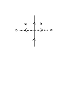
Figure 1: The pion–pion–nucleon vertex from Eq. (49). Here $q^{\mu}\equiv p^{\mu}_{i}-p^{\mu}_{f}-k^{\mu}$, in terms of the initial and final nucleon four-momenta and the outgoing pion four-momentum $k^{\mu}$.

Figure 2: The pion–nucleon vertex from Eq. (49). Here $q^{\mu}\equiv p^{\mu}_{i}-p^{\mu}_{f}$.

To lowest order in the pion field, the Noether axial current due to ${\cal L}_{2}$ takes the form

$$A^{a\mu}_{2}=-{1\over f_{\pi}}\,\epsilon^{abc}\pi^{b}\,{\overline{N\mkern 3.0mu}\mkern-3.0mu}{}\mkern 2.0mu\gamma^{\mu}{\tau^{c}\over 2}\,N-g_{A}\,{\overline{N\mkern 3.0mu}\mkern-3.0mu}{}\mkern 2.0mu\gamma^{\mu}\gamma_{5}{\tau^{a}\over 2}\,N-f_{\pi}\,{\partial}^{\mu}{\pi}^{a}+O({\pi}^{2})\ .$$ (50)

To determine the Feynman rules for the axial-current vertices, we consider a lagrangian density

$${\cal L}_{\mathrm{ext}}(x)=A^{a\mu}(x)\,S^{\mathrm{ext}}_{a\mu}(x)\ ,$$ (51)

where $S^{\mathrm{ext}}_{a\mu}$ is an external source that could originate from leptons, for example. The scattering matrix $S_{fi}$ can then be written to first order in the external source as

$$S^{\mkern 2.0mu(1)}_{fi}=\left(\>\prod_{\mathrm{bosons}}{1\over(2\omega_{b}{\mathbb{V}})^{1/2}}\right)\left(\>\prod_{\mathrm{fermions}}{1\over(2E_{f}{\mathbb{V}})^{1/2}}\right)M^{a\mu}(k)\,{\widetilde{S}}^{\mathrm{ext}}_{a\mu}(k)\ ,$$ (52)

which defines the covariant amplitude $M^{a\mu}(k)$. Here $\omega_{b}$ are the boson energies, $E_{f}$ are the fermion energies, and $\mathbb{V}$ is the quantization volume; these factors specify the normalization to be used on external lines. The fermion spinors are included in $M^{a\mu}$, which is to be computed using the Feynman rules with the axial-current vertices given below; we assume overall four-momentum conservation (as well as four-momentum conservation at every vertex), and we adopt the covariant spinor normalization $\bar{u}(p)u(p)=-\bar{v}(p)v(p)=2M$.

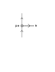
Figure 3: The nucleon–pion vertex in the axial current (50), from Eq. (53). The crossed circle shows where and how to attach the external source ${\widetilde{S}}^{\mathrm{ext}}_{a\mu}(k)$.

Figure 4: The vertex for the nucleon-only term in the axial current (50), from Eq. (53).

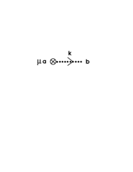
Figure 5: The vertex for the pionic contribution to the axial current (50), from Eq. (53).

The vertices arising from Eqs. (50) to (52) are given by

$$-{i\over f_{\pi}}\,\epsilon^{abc}\gamma^{\mu}{\tau^{c}\over 2}\ ,\qquad-i{g_{A}}\mkern 2.0mu\gamma^{\mu}\gamma_{5}{\tau^{a}\over 2}\ ,\qquad f_{\pi}k^{\mu}{\delta}^{ab}\ ,$$ (53)

and they are represented diagrammatically in Figs. 3, 4, and 5, respectively.

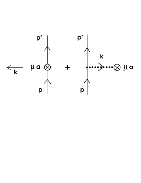
Figure 6: The leading-order, one-body, axial-vector current. Note that the external source ${\widetilde{S}}^{\mathrm{ext}}_{a\mu}(k)$ “extracts” the momentum $k^{\mu}$ from both diagrams: explicitly when the pion leaves the diagram and implicitly when the source attaches directly to the nucleon line.

The one-body, axial-current matrix element to lowest order in $1/f_{\pi}$ is given by

$$M^{a\mu}(1)=ig_{A}\>\bar{u}(p^{\prime}){\gamma}_{5}\left\{{\gamma}^{\mu}-\hbox to0.0pt{/\hss}{\mkern-1.0muk}{{k^{\mu}}\over{k^{2}-m^{2}_{\pi}}}\right\}{{{\tau}^{a}}\over 2}\,u(p)\ .$$ (54)

The two relevant Feynman diagrams are drawn in Fig. 6, where $k^{\mu}$ is the outgoing momentum on the pion line. Note that the multiplicative factor of $g_{A}$ in the amplitude implies that no additional current renormalization is required. Here $g_{A}$ enters as an overall factor, which was missing in the tree-diagram amplitude calculated in the $\sigma\omega$ model of Ref. Ana98 :

$$M^{a\mu}(1)=g_{A}\>M^{a\mu}_{\sigma\omega}(1)\ .$$ (55)

The interaction amplitude (54) satisfies PCAC automatically, due to the presence of the projection operator in braces:

$$k_{\mu}M^{a\mu}(1)\lower 8.1805pt\vbox{\hbox{$\ \buildrel{\hbox{\Large\rightarrowfill}}\over{\scriptstyle{m_{\pi}\,\rightarrow\,0}}\ $}}\,0\ .$$ (56)

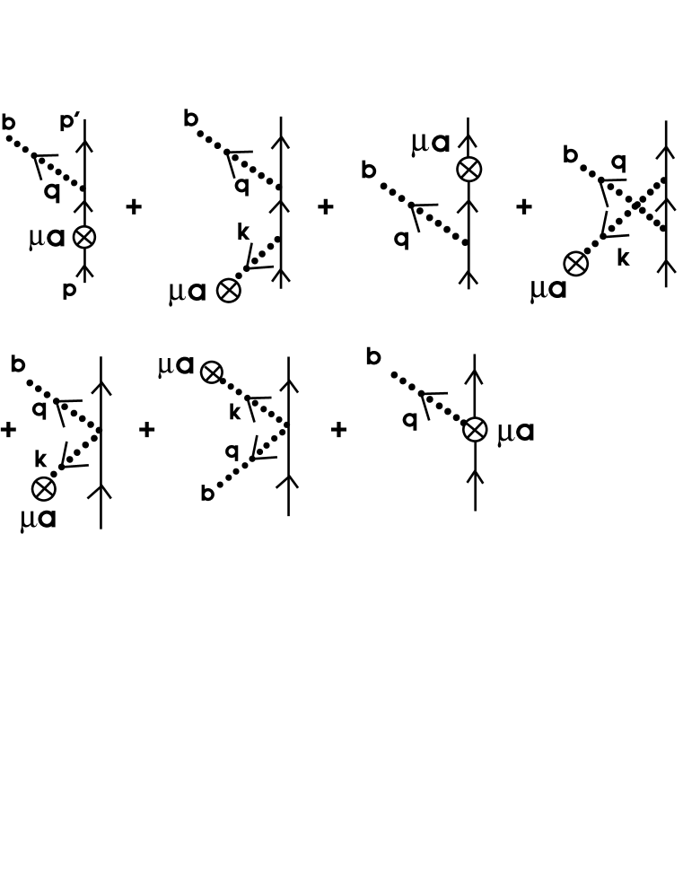
Figure 7: The amplitude for axial-current pion production on a single nucleon [Eq. (57)]. Again, note that $k^{\mu}$ is extracted by the external source, so that $p^{\mu}={p^{\prime}}^{\mu}+k^{\mu}+q^{\mu}$.

The amplitude for axial-current pion production on a single nucleon is represented by the diagrams of Fig. 7 and can be written as

$$2f_{\pi}\>M^{ab\,\mu}(\pi) = \bar{u}(p^{\prime})\left\{g^{2}_{A}\left[\not\!q\,{\gamma}_{5}\,{1\over{(\not\!p^{\mkern 2.0mu\prime}\,+\not\!q)-M}}\,{\gamma}_{5}\left({\gamma}^{\mu}-\not\!k{{{k}^{\mu}}\over{k^{2}-m_{\pi}^{2}}}\right){{{\tau}^{b}{\tau}^{a}}\over 2}\right.\right.$$ (57)

$$\qquad\qquad\qquad\quad+\left.\left({\gamma}^{\mu}-\not\!{k}{{k^{\mu}}\over{k^{2}-m_{\pi}^{2}}}\right){\gamma}_{5}{1\over{(\not\!p\;-\not\!q)-M}}\,{\gamma}_{5}\!\not\!q\,{{{\tau}^{a}{\tau}^{b}}\over 2}\right]$$

$$\qquad\qquad+\left.i{\epsilon}^{abc}\,{{{\tau}^{c}}\over 2}\left[(\not\!k\,-\!\not\!q){{k^{\mu}}\over{k^{2}-m_{\pi}^{2}}}-2{\gamma}^{\mu}\right]\right\}u(p)\ ,$$

where $q^{\mu}$ is the outgoing four-momentum of the emitted pion, and $p^{\mu}$ and ${p^{\prime}}^{\mu}$ are the initial and final nucleon four-momenta, respectively. It is easy to verify that this amplitude satisfies PCAC (for an on-shell nucleon).

In the soft-pion limit $(q,k\rightarrow 0)$ and to leading order in $1/M$,

$${1\over{{\mathbb{V}}{(2E\,2E^{\prime})}^{1/2}}}\>iM^{ab\,\mu}(\pi)\longrightarrow{1\over{f_{\pi}}}\>{\epsilon}^{abc}\,{{\tau}^{c}\over 2}\>{\delta}^{\mu 0}\ ,$$ (58)

where $E\approx E^{\prime}\approx M$ are the initial and final energies of the nucleons, and the arrow signifies that we have removed the external nonrelativistic wave functions (including a factor of $1/\sqrt{\mathbb{V}}\,$) to arrive at a first-quantized operator. This amplitude reproduces the result of Kubodera, Delorme, and Rho (KDR) Kub78 obtained in the current-algebra approach and solves the problem of an extra factor of $g^{2}_{A}$ found in Ref. Ana98 .

Next we consider amplitudes for the axial current that involve two nucleons. The relevant diagrams to this order in $\nu$ are presented in Fig. 8 (with a similar set of diagrams when the external source interacts with the second nucleon) and produce an amplitude of the form

$$M^{a\mu}(2)=M^{ab\>\mu}(\pi)\;{i\over{q^{2}-m_{\pi}^{2}}}\;\,{{g_{A}}\over{f_{\pi}}}\;\bar{u}(p^{\prime}_{2})\not\!q\,{\gamma}_{5}\,{{{\tau}^{b}}\over 2}\,u(p_{2})+\mathrm{(direct)}_{2}+\mathrm{cross\ terms.}$$ (59)

Here “$\mathrm{(direct)}_{2}$” denotes the terms where the external source hits nucleon 2, and “cross terms” denotes similar diagrams with the fermion lines crossed in the final state.

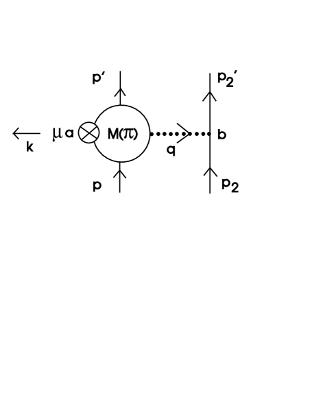
Figure 8: Two-nucleon contributions to the axial current. Here the vertex $M(\pi)$ [Eq. (57)] represents all possible ways that the external source can couple to the left-hand nucleon line (to the order we are working), as illustrated in Fig. 7.

This amplitude satisfies PCAC because $M^{ab\>\mu}(\pi)$ does. The corresponding two-body nuclear AXC can be identified to lowest order in the inverse nucleon mass $M$ from an expression for the $S$-matrix element:

$${A}_{\mathrm{eff}}^{a\mu}(2)\equiv-{1\over{{(2M\,{\mathbb{V}})}^{2}}}\,iM^{a\mu}(2)\ .$$ (60)

By performing a nonrelativistic reduction of the direct terms in the resulting current, and by removing factors for the external nonrelativistic wave functions, one obtains

$$A_{\mathrm{eff}}^{a0}({\bf q},{\bf Q})\longrightarrow{g_{A}\over{4f_{\pi}^{2}}}\;i\,{\left[\mbox{\boldmath$\tau$}(1)\mbox{\boldmath${}\times\tau$}(2)\right]}^{a}\;\left\{{{\mbox{\boldmath$\sigma$}}(2)\mbox{\boldmath$\,\cdot\,$}{{\bf q}}\over{{{\bf q}}^{2}+m_{\pi}^{2}}}-{{\mbox{\boldmath$\sigma$}}(1)\mbox{\boldmath$\,\cdot\,$}{{\bf Q}}\over{{{\bf Q}}^{2}+m_{\pi}^{2}}}\right\}\ ,$$ (61)

where the exchanged momenta are defined by ${\mathbf{q}}\equiv{\mathbf{p}}^{\prime}_{2}-{\mathbf{p}}_{2}$ and ${\mathbf{Q}}\equiv{\mathbf{p}}^{\prime}-{\mathbf{p}}$.

This is the same two-body, axial charge density obtained by KDR Kub78 in the current-algebra approach. Here, however, this result has been calculated as the lowest-order approximation to an EFT lagrangian. The lagrangian approach allows us to explicitly calculate additional contributions to this AXC from the next-to-leading-order ($\nu=3$) terms in the NDA counting scheme.

IV Relevant Terms with $\ \nu=3$

We now concentrate on the contributions from the $\nu=3$ terms in the lagrangian. Since our ultimate objective is to identify axial-vector exchange currents arising from Eq. (2) to lowest order in the meson fields, we consider only terms that contribute to the vector and axial-vector currents to this order in $\nu$. These terms are bilinear in derivatives of the pion field itself, but contain the field to all orders. We obtain the $\nu=3$ lagrangian

$${\cal L}_{3}={\delta}_{1}{\cal L}+{\delta}_{2}{\cal L}\ ,$$ (62)

where

$${\delta}_{1}{\cal L}\equiv-{{{\kappa}_{\pi}}\over M}\,{\overline{N\mkern 3.0mu}\mkern-3.0mu}{}\mkern 2.0mu{v}_{\mu\nu}{\sigma}^{\mu\nu}N$$ (63)

and

$${\delta}_{2}{\cal L}\equiv{{4{\beta}_{\pi}}\over M}\,{\overline{N\mkern 3.0mu}\mkern-3.0mu}{}\mkern 2.0muN\,{\rm Tr}\left(a_{\mu}a^{\mu}\right)\ ,$$ (64)

with $v_{\mu\nu}$ given by Eq. (8), and $a_{\mu}$ given by Eq. (4). The final term contributing to the two-body axial current at relevant order in $\nu$ involves the $\rho$ meson field:

$${\cal L}_{\rho} \equiv {-g_{\rho}}{\overline{N\mkern 3.0mu}\mkern-3.0mu}{}\mkern 2.0mu{\rho}_{\mu}{\gamma}^{\mu}N-{{f_{\rho}g_{\rho}}\over{4M}}\,{\overline{N\mkern 3.0mu}\mkern-3.0mu}{}\mkern 2.0mu{\rho}_{\mu\nu}{\sigma}^{\mu\nu}N-{1\over 2}\,{\rm Tr}\left({\rho}_{\mu\nu}{\rho}^{\mu\nu}\right)$$ (65)

$$\quad{-g_{\rho\pi\pi}}\,{{2f^{2}_{\pi}}\over{m^{2}_{\rho}}}\,{\rm Tr}\left({\rho}_{\mu\nu}{v}^{\mu\nu}\right)+m^{2}_{\rho}\,{\rm Tr}\left({\rho}_{\mu}{\rho}^{\mu}\right)\ ,$$

where $\rho_{\mu\nu}$ is defined in Eqs. (10) and (11). Here the first and last terms are of order $\nu=2$, the second term is of order $\nu=3$, and the third and fourth terms are of order $\nu=4$. The fourth term is included in ${\cal L}_{\rho}$ because it is the lowest-order term that involves $\rho\pi$ interactions, which are thought to be relevant in AXC originating from heavy mesons Iva79 . We first consider the terms in Eqs. (63) and (64), which describe the interaction of nucleons with pions, and then return to calculate the additional contributions due to the $\rho$ meson field in Sec. VI.

One can calculate the change in ${\cal L}_{3}$ under vector or axial-vector transformations. These quantities are required for calculating the respective Noether currents according to the definition (24):

$$\delta{\cal L}_{3}={{{2i\kappa}_{\pi}}\over{M}}\,{\overline{N\mkern 3.0mu}\mkern-3.0mu}{}\mkern 2.0mu\left[\delta a_{\mu},\>a_{\nu}\right]{\sigma}^{\mu\nu}N+{{8{\beta}_{\pi}}\over{M}}\,{\overline{N\mkern 3.0mu}\mkern-3.0mu}{}\mkern 2.0muN\>{\rm Tr}\left(\delta a_{\mu}\,a^{\mu}\right)+O\left((\delta a)^{2}\right)\ ,$$ (66)

where $\delta a_{\mu}$ is different for the (local) vector and axial-vector transformations:

$$\delta a_{\mu} = {1\over 4}\left({\xi}^{{\dagger}}{\tau}^{a}\xi-\xi{\tau}^{a}{\xi}^{{\dagger}}\right){\partial}_{\mu}{\beta}^{a}\qquad\mathrm{vector},$$ (67)

$$\delta a_{\mu} = {1\over 4}\left({\xi}^{{\dagger}}{\tau}^{a}\xi+\xi{\tau}^{a}{\xi}^{{\dagger}}\right){\partial}_{\mu}{\alpha}^{a}\qquad\mathrm{axial\ vector}.$$ (68)

These variations produce the following Noether currents, as defined in Eq. (24):

$$V^{a\mu}_{3}=-{{i{\kappa}_{\pi}}\over{2M}}\>{\overline{N\mkern 3.0mu}\mkern-3.0mu}{}\mkern 2.0mu{\sigma}^{\mu\nu}\left[{\xi}^{{\dagger}}{\tau}^{a}\xi-\xi{\tau}^{a}{\xi}^{{\dagger}},\>a_{\nu}\right]N-{{2{\beta}_{\pi}}\over{M}}\>{\overline{N\mkern 3.0mu}\mkern-3.0mu}{}\mkern 2.0muN\>{\rm Tr}\left[({\xi}^{{\dagger}}{\tau}^{a}\xi-\xi{\tau}^{a}{\xi}^{{\dagger}})\>a^{\mu}\right]\ ,$$ (69)

$$A^{a\mu}_{3}=-{{i{\kappa}_{\pi}}\over{2M}}\>{\overline{N\mkern 3.0mu}\mkern-3.0mu}{}\mkern 2.0mu{\sigma}^{\mu\nu}\left[{\xi}^{{\dagger}}{\tau}^{a}\xi+\xi{\tau}^{a}{\xi}^{{\dagger}},\>a_{\nu}\right]N-{{2{\beta}_{\pi}}\over{M}}\>{\overline{N\mkern 3.0mu}\mkern-3.0mu}{}\mkern 2.0muN\>{\rm Tr}\left[({\xi}^{{\dagger}}{\tau}^{a}\xi+\xi{\tau}^{a}{\xi}^{{\dagger}})\>a^{\mu}\right]\ .$$ (70)

For future reference, we exhibit some often-encountered expressions as functions of the pion field:

$$\left({\xi}^{{\dagger}}{\tau}^{a}\xi+\xi{\tau}^{a}{\xi}^{{\dagger}}\right)=2{\tau}^{b}\left({\rm cos}\left({{\pi}\over{f_{\pi}}}\right)\left[{\delta}^{ab}-\hat{\pi}^{a}\hat{\pi}^{b}\right]+\hat{\pi}^{a}\hat{\pi}^{b}\right)\ ,$$ (71)

$$\left({\xi}^{{\dagger}}{\tau}^{a}\xi-\xi{\tau}^{a}{\xi}^{{\dagger}}\right)=-2{\epsilon}^{abc}\hat{\pi}^{b}{\tau}^{c}\>{\rm sin}\left({{\pi}\over{f_{\pi}}}\right)\ ,$$ (72)

$$a_{\mu}={{1}\over{2f_{\pi}}}\,{\tau}^{c}\,{\partial}_{\mu}{\pi}^{d}\left\{A_{1}(\pi)\left[{\delta}^{cd}-\hat{\pi}^{c}\hat{\pi}^{d}\right]+\hat{\pi}^{c}\hat{\pi}^{d}\right\}\ ,$$ (73)

where $A_{1}(\pi)$ is defined in Eq. (22). By substituting these relations into Eq. (69), the extra vector current can be written in terms of pion fields as

$$V^{a\mu}_{3} = {1\over{{\pi}M}}\,{\epsilon}^{abc}\,\hat{\pi}^{b}\,{\partial}_{\nu}{\pi}^{m}\,{\rm sin}^{2}\left({{\pi}\over{f_{\pi}}}\right)$$

$$\quad\times\left\{-{\kappa}_{\pi}\,{\epsilon}^{cdn}\left(\left[{\delta}^{dm}-\hat{\pi}^{d}\hat{\pi}^{m}\right]+{{1}\over{A_{1}(\pi)}}\,\hat{\pi}^{d}\hat{\pi}^{m}\right){\overline{N\mkern 3.0mu}\mkern-3.0mu}{}\mkern 2.0mu{\sigma}^{\mu\nu}{\tau}^{n}N+4{\beta}_{\pi}\,{\delta}^{cm}{\overline{N\mkern 3.0mu}\mkern-3.0mu}{}\mkern 2.0muNg^{\mu\nu}\right\}\ .$$

For the additional axial current (70), one obtains

$$A^{a\mu}_{3} = {1\over{f_{\pi}M}}\left\{{\kappa}_{\pi}\,{\epsilon}^{bcd}\,{\overline{N\mkern 3.0mu}\mkern-3.0mu}{}\mkern 2.0mu{\tau}^{d}{\sigma}^{\mu\nu}N-4{\beta}_{\pi}\,{\delta}^{bc}\,{\overline{N\mkern 3.0mu}\mkern-3.0mu}{}\mkern 2.0muNg^{\mu\nu}\right\}{\partial}_{\nu}{\pi}^{m}$$ (75)

$$\quad\times\left({\rm cos}\left({{\pi}\over{f_{\pi}}}\right)\left[{\delta}^{ab}-\hat{\pi}^{a}\hat{\pi}^{b}\right]+\hat{\pi}^{a}\hat{\pi}^{b}\right)\left\{A_{1}(\pi)\left[{\delta}^{cm}-\hat{\pi}^{c}\hat{\pi}^{m}\right]+\hat{\pi}^{c}\hat{\pi}^{m}\right\}\ .$$

Now one can construct the corresponding total charge densities used to check the chiral algebra of charges. For the vector charge density, one finds

$$V^{a0} = V^{a0}_{\pi}+V^{a0}_{\pi N}+V^{a0}_{3}$$ (76)

$$= A_{1}^{2}(\pi)\>{\epsilon}^{abc}{\pi}^{b}\left(1+{{4{\beta}_{\pi}}\over{f_{\pi}^{2}M}}\,{\overline{N\mkern 3.0mu}\mkern-3.0mu}{}\mkern 2.0muN\right){\partial}_{0}{\pi}^{c}+N^{{\dagger}}{{{\tau}^{b}}\over 2}N\>\left[{\rm cos}\left({{\pi}\over{f_{\pi}}}\right)\left({\delta}^{ab}-\hat{\pi}^{a}\hat{\pi}^{b}\right)+\hat{\pi}^{a}\hat{\pi}^{b}\right]$$

$$\quad{}+g_{A}\>{\epsilon}^{abc}\>\hat{\pi}^{b}\>{\rm sin}\left({{\pi}\over{f_{\pi}}}\right)N^{{\dagger}}{\gamma}_{5}{{{\tau}^{c}}\over 2}N$$

$$\quad{}-{{{\kappa}_{\pi}}\over{f_{\pi}^{2}M}}\,{\epsilon}^{abc}\,{\pi}^{b}A_{1}^{2}(\pi)\,{\partial}_{i}{\pi}^{m}{\epsilon}^{cdn}\left(\left[{\delta}^{dm}-\hat{\pi}^{d}\hat{\pi}^{m}\right]+{{1}\over{A_{1}(\pi)}}\,\hat{\pi}^{d}\hat{\pi}^{m}\right){\overline{N\mkern 3.0mu}\mkern-3.0mu}{}\mkern 2.0mu{\sigma}^{0i}{\tau}^{n}N\ ,$$

while the corresponding axial-vector charge density is

$$A^{a0} = A^{a0}_{\pi}+A^{a0}_{\pi N}+A^{a0}_{3}$$ (77)

$$= -f_{\pi}^{2}\left(1+{{4{\beta}_{\pi}}\over{f_{\pi}^{2}M}}\,{\overline{N\mkern 3.0mu}\mkern-3.0mu}{}\mkern 2.0muN\right){\partial}_{0}{\pi}^{b}\left\{{1\over{\pi}}\,{\rm sin}\left({{\pi}\over{f_{\pi}}}\right){\rm cos}\left({{\pi}\over{f_{\pi}}}\right)\left({\delta}^{ab}-\hat{\pi}^{a}\hat{\pi}^{b}\right)+{1\over{f_{\pi}}}\,\hat{\pi}^{a}\hat{\pi}^{b}\right\}$$

$$\quad{}-{\epsilon}^{abc}\>\hat{\pi}^{b}\>{\rm sin}\left({{\pi}\over{f_{\pi}}}\right)N^{{\dagger}}{{{\tau}^{c}}\over 2}N-{g_{A}}\mkern 2.0muN^{{\dagger}}{\gamma}_{5}{{{\tau}^{b}}\over 2}N\left[{\rm cos}\left({{\pi}\over{f_{\pi}}}\right)\left({\delta}^{ab}-\hat{\pi}^{a}\hat{\pi}^{b}\right)+\hat{\pi}^{a}\hat{\pi}^{b}\right]$$

$$\quad{}+{{{\kappa}_{\pi}}\over{f_{\pi}M}}\,{\epsilon}^{bcd}\,{\overline{N\mkern 3.0mu}\mkern-3.0mu}{}\mkern 2.0mu{\sigma}^{0i}{\tau}^{d}N\>{\partial}_{i}{\pi}^{m}$$

$$\qquad\quad\times\left({\rm cos}\left({{\pi}\over{f_{\pi}}}\right)\left[{\delta}^{ab}-\hat{\pi}^{a}\hat{\pi}^{b}\right]+\hat{\pi}^{a}\hat{\pi}^{b}\right)\left\{A_{1}(\pi)\left[{\delta}^{cm}-\hat{\pi}^{c}\hat{\pi}^{m}\right]+\hat{\pi}^{c}\hat{\pi}^{m}\right\}\ .$$

The factor $\left(1+4{\beta}_{\pi}{\overline{N\mkern 3.0mu}\mkern-3.0mu}{}\mkern 2.0muN/{f_{\pi}^{2}M}\right)$ in the first term of both densities represents the net effect of the ${\delta}_{2}{\cal L}$ term in the lagrangian ${\cal L}_{3}$, which is proportional to ${\beta}_{\pi}$. It is interesting that the same factor times ${\partial}_{0}{\pi}^{a}$ can be readily expressed in terms of the pion canonical momentum, when one inverts the full expression for the momentum, including the contributions of the new pion–nucleon terms in the lagrangian. Thus one finds

$$\Big{(}1 + {{4{\beta}_{\pi}}\over{f_{\pi}^{2}M}}\,{\overline{N\mkern 3.0mu}\mkern-3.0mu}{}\mkern 2.0muN\Big{)}{\partial}_{0}{\pi}^{a}$$

$$\quad{}=\left[{1\over{A_{1}^{2}(\pi)}}\left({\delta}^{ab}-\hat{\pi}^{a}\hat{\pi}^{b}\right)+\hat{\pi}^{a}\hat{\pi}^{b}\right]P^{b}_{\pi}-{\epsilon}^{abc}\,{1\over{A_{1}^{2}(\pi)}}\,{\pi}^{b}{1\over{{\pi}^{2}}}\,{\rm sin}^{2}\left({{\pi}\over{2f_{\pi}}}\right)\,N^{{\dagger}}{\tau}^{c}N$$

$$\qquad{}-{1\over{2f_{\pi}}}\,g_{A}\left[{1\over{A_{1}(\pi)}}\left({\delta}^{ab}-\hat{\pi}^{a}\hat{\pi}^{b}\right)+\hat{\pi}^{a}\hat{\pi}^{b}\right]N^{{\dagger}}{\gamma}_{5}{\tau}^{b}N$$

$$\qquad{}+{{{\kappa}_{\pi}}\over{f_{\pi}^{2}}M}\left({\epsilon}^{anc}-{{A_{1}(\pi)-1}\over{A_{1}(\pi)}}\,{\epsilon}^{abc}\,\hat{\pi}^{b}\hat{\pi}^{n}+[A_{1}(\pi)-1]\,{\epsilon}^{bnc}\,\hat{\pi}^{a}\hat{\pi}^{b}\right){\partial}_{i}{\pi}^{n}{\overline{N\mkern 3.0mu}\mkern-3.0mu}{}\mkern 2.0mu{\sigma}^{0i}{\tau}^{c}N\ ,$$

and the additional lagrangian ${\delta}_{2}{\cal L}$ proportional to ${\beta}_{\pi}$ has no effect on the full charges, when they are written in terms of canonical momenta.

By substituting the relation (LABEL:eq:full-pi-momentum) into Eqs. (76) and (77) for the vector and axial-vector charge densities, and by carrying out the necessary algebra, one remarkably arrives at precisely the same expressions for the charge densities in terms of the canonical momenta [Eqs. (44) and (45)] as those obtained with no $\nu=3$ terms included! Thus the expressions for the Noether charges in terms of canonical momenta are not influenced by the presence of the term proportional to ${\kappa}_{\pi}$ either. Note, however, that these $\nu=3$ terms will generally influence the three-vector currents.

Since Eqs. (44) and (45) are known to satisfy the correct chiral charge algebra, we conclude that the $\nu=3$ pion–nucleon terms in the lagrangian do not influence the charge algebra whatsoever.

V interaction amplitudes to order $\ \nu=3$

To lowest order in the pion field, the Noether axial current (75) can be written as

$$A^{a\mu}_{3}\approx{{{\kappa}_{\pi}}\over{f_{\pi}M}}\,{\epsilon}^{abc}\>{\partial}_{\nu}{\pi}^{b}\>{\overline{N\mkern 3.0mu}\mkern-3.0mu}{}\mkern 2.0mu{\tau}^{c}{\sigma}^{\mu\nu}N-{{4{\beta}_{\pi}}\over{f_{\pi}M}}\>{\overline{N\mkern 3.0mu}\mkern-3.0mu}{}\mkern 2.0muN\>{\partial}^{\mu}{\pi}^{a}+\cdots\ .$$ (79)

We calculate additional contributions to the interaction amplitudes originating from the lagrangians (63) and (64) separately. We first need to find the corresponding interaction vertices, and we begin by considering ${\delta}_{1}{\cal L}$. Recall that to lowest order in the pion field,

$$a_{\nu}\approx{1\over{2f_{\pi}}}\,\mbox{\boldmath$\tau\,\cdot$}\,{\partial}_{\nu}\mbox{\boldmath$\pi$}+\cdots\ ,$$ (80)

$$v_{\mu\nu}\approx{{1}\over{f_{\pi}^{2}}}\,{\epsilon}^{abc}\,{\partial}_{\mu}{\pi}^{a}{\partial}_{\nu}{\pi}^{b}\,{{{\tau}^{c}}\over{2}}+\cdots\ .$$ (81)

The extra term produces a new lowest-order, strong-interaction vertex that looks exactly like the one in Fig. 1, but which corresponds now to an analytical expression

$${{2i{\kappa}_{\pi}}\over{f_{\pi}^{2}M}}\,{\epsilon}^{abc}\,{{{\tau}^{c}}\over{2}}\,k_{\mu}q_{\nu}{\sigma}^{\mu\nu}\ .$$ (82)

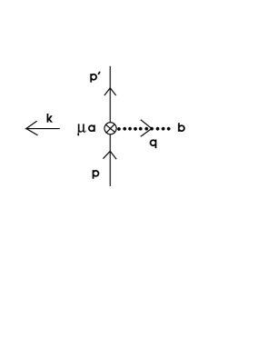
Figure 9: The vertex for the one-body axial current arising from ${\delta}_{1}{\cal L}$. Here $p^{\mu}=q^{\mu}+k^{\mu}+{p^{\prime}}^{\mu}$.

The one-nucleon, axial-current interaction vertex due to ${\delta}_{1}{\cal L}$ (see Fig. 9) follows from the first term in Eq. (79):

$${}-{{2{\kappa}_{\pi}}\over{f_{\pi}M}}\,{\epsilon}^{abc}\,q_{\nu}{\sigma}^{\mu\nu}\,{{{\tau}^{c}}\over{2}}\ .$$ (83)

This vertex gives an additional amplitude for axial-current pion production on a single nucleon that resembles the last two diagrams in Fig. 7 and corresponds to the expression

$$M^{ab\>\mu}(\pi)={}-{1\over{f_{\pi}}}{{2{\kappa}_{\pi}}\over{M}}\,{\epsilon}^{abc}\left\{g^{\mu}_{{\phantom{\mu}}\lambda}-{{k^{\mu}k_{\lambda}}\over{k^{2}-m_{\pi}^{2}}}\right\}\>q_{\nu}\,\bar{u}(p^{\prime})\,{\sigma}^{\lambda\nu}\,{{{\tau}^{c}}\over{2}}\,u(p)\ .$$ (84)

This amplitude satisfies PCAC because

$$k_{\mu}\>M^{ab\>\mu}(\pi)\propto\left\{k_{\lambda}-{{k^{2}}\over{k^{2}-m_{\pi}^{2}}}k_{\lambda}\right\}\,\lower 8.1805pt\vbox{\hbox{$\ \buildrel{\hbox{\Large\rightarrowfill}}\over{\scriptstyle{m_{\pi}\,\rightarrow\,0}}\ $}}\,0\ .$$ (85)

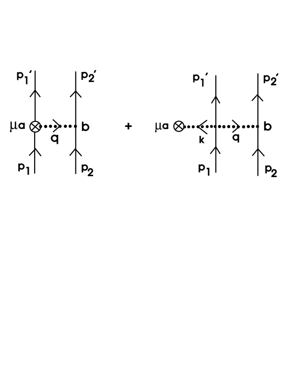
Figure 10: Two-nucleon, axial-current amplitude originating from ${\delta}_{1}{\cal L}$ [Eq. (86)].

By combining all of the previous results, one can calculate an additional two-nucleon, axial-current interaction amplitude due to the ${\delta}_{1}{\cal L}$ term (see Fig. 10):

$$M^{a\mu}(2) = {}-i\,{{g_{A}}\over{f_{\pi}^{2}}}{{2{\kappa}_{\pi}}\over{M}}\,{\epsilon}^{abc}\left\{g^{\mu}_{{\phantom{\mu}}\lambda}-{{k^{\mu}k_{\lambda}}\over{k^{2}-m_{\pi}^{2}}}\right\}\>\left[\bar{u}(p_{1}^{\prime}){\sigma}^{\lambda\nu}\,{{{\tau}^{c}}\over{2}}\,u(p_{1})\right.$$ (86)

$$\quad{}\times\left.{{q_{\nu}q_{\sigma}}\over{q^{2}-m_{\pi}^{2}}}\>\bar{u}(p_{2}^{\prime}){\gamma}^{\sigma}{\gamma}_{5}\,{{{\tau}^{b}}\over{2}}\,u(p_{2})+(\mathrm{direct})_{2}+\mathrm{cross\ terms}\right]\ .$$

Here “$(\mathrm{direct})_{2}$” again denotes contributions from diagrams where the axial-current vertex resides on the second nucleon, which can be obtained from the first term by the replacements $p_{1}\leftrightarrow p_{2}$, $p^{\prime}_{1}\leftrightarrow p^{\prime}_{2}$, and $q\to Q$, and “cross terms” denotes similar diagrams in which the fermion lines are crossed in the final state. This amplitude produces the first additional contribution to the nuclear AXC originating from the ${\cal L}_{3}$ terms in the EFT lagrangian.

Now recall that there is yet another term (64) in the $\nu=3$, pion–nucleon lagrangian that can be written to lowest order in the pion field as

$${\delta}_{2}{\cal L}\approx{2\beta_{\pi}\over f^{2}_{\pi}M}\,{\overline{N\mkern 3.0mu}\mkern-3.0mu}{}\mkern 2.0muN\,{\partial}_{\mu}{\pi}^{a}{\partial}^{\mu}{\pi}^{a}\ .$$ (87)

The corresponding vertex again looks like that in Fig. 1 but now represents an analytical expression

$$-{{4i{\beta}_{\pi}}\over{f_{\pi}^{2}M}}\,k_{\mu}q^{\mu}{\delta}^{ab}\ .$$ (88)

The one-nucleon, axial-current interaction vertex looks the same as in Fig. 9 and can be deduced from the second term in Eq. (79) to be

$${{4{\beta}_{\pi}}\over{f_{\pi}M}}\,q^{\mu}{\delta}^{ab}\ .$$ (89)

It is easy to write out a corresponding axial-current, pion-production amplitude (again resembling the last two diagrams in Fig. 7):

$$M^{ab\>\mu}(\pi)={{4{\beta}_{\pi}}\over{f_{\pi}M}}\left\{q^{\mu}-{{k^{\mu}}\over{k^{2}-m_{\pi}^{2}}}\,k\cdot q\right\}{\delta}^{ab}\,\bar{u}(p^{\prime})u(p)\ .$$ (90)

This amplitude also satisfies PCAC:

$$k_{\mu}\,M^{ab\>\mu}(\pi)\propto\left\{k\cdot q-{{k^{2}}\over{k^{2}-m_{\pi}^{2}}}\,k\cdot q\right\}\,\lower 8.1805pt\vbox{\hbox{$\ \buildrel{\hbox{\Large\rightarrowfill}}\over{\scriptstyle{m_{\pi}\,\rightarrow\,0}}\ $}}\,0\ .$$ (91)

The corresponding two-nucleon, axial-current interaction allows one to identify additional contributions to the axial two-body amplitude originating from the ${\delta}_{2}{\cal L}$ term in the lagrangian. (They also look like Fig. 10.) One obtains

$$M^{a\mu}(2)=i\,{{g_{A}}\over{f_{\pi}^{2}}}{{4{\beta}_{\pi}}\over{M}}\left\{q^{\mu}-{{k^{\mu}}\over{k^{2}-m_{\pi}^{2}}}\,k\cdot q\right\}{q_{\sigma}\over{q^{2}-m_{\pi}^{2}}}\>\left[\bar{u}(p^{\prime}_{1})u(p_{1})\>\bar{u}(p_{2}^{\prime}){\gamma}^{\sigma}{\gamma}_{5}\,{{{\tau}^{a}}\over{2}}\,u(p_{2})\right.$$

$$\hskip 195.12877pt{}+(\mathrm{direct})_{2}+{}\mathrm{cross\ terms}\,\bigg{]}\ .\$$ (92)

The sum of the amplitudes (86) and (92) constitutes the total contribution of the pion–nucleon $\nu=3$ terms in the EFT lagrangian to the AXC.

VI rho meson terms in the EFT lagrangian

VI.1 Currents and canonical momenta

An additional piece in the EFT lagrangian (65) contains the rho meson field

$${\rho}_{\mu}(x)\equiv{{1}\over{2}}\,\mbox{\boldmath$\tau\cdot\rho$}_{\mu}(x)\ ,$$ (93)

which behaves under a chiral transformation as

$${\rho}_{\mu}^{\prime}(x)=h(x){\rho}_{\mu}(x)h^{{\dagger}}(x)\ .$$ (94)

In principle, one can confirm the same chiral charge algebra as before to all orders in the pion field. This follows just as in the case of the pionic interactions: the contributions of extra pieces in the lagrangian are absorbed in the modified pion canonical momentum. To simplify the subsequent equations, however, we present the proof only to lowest order in the pion field.

For infinitesimal vector transformations,

$${{\partial\!\left(\delta{\rho}_{\mu}^{c}\right)}\over{\partial{\beta}^{a}}}=-{\epsilon}^{abc}{\rho}_{\mu}^{b}\ ,$$ (95)

while for infinitesimal axial transformations,

$${{\partial\!\left(\delta{\rho}_{\mu}^{f}\right)}\over{\partial{\alpha}^{a}}}={1\over{2f_{\pi}}}\,{\epsilon}^{abc}{\epsilon}^{cdf}{\pi}^{b}{\rho}_{\mu}^{d}\ .$$ (96)

One also recalls that to lowest order in pion fields,

$$v_{\mu}\approx{{1}\over{2f_{\pi}^{2}}}\,{\epsilon}^{abc}{\pi}^{a}\,{\partial}_{\mu}{\pi}^{b}\,{{{\tau}^{c}}\over 2}\ .$$ (97)

Additional terms in the EFT lagrangian due to the presence of the rho meson are given by ${\cal L}_{\rho}$ in Eq. (65). To lowest relevant order in the meson fields, one obtains the following strong-interaction vertices for the $\rho$ meson:

$$-ig_{\rho}{{{\tau}^{c}}\over 2}\left({\gamma}^{\lambda}+{{f_{\rho}}\over{2M}}\,iq_{\nu}{\sigma}^{\nu\lambda}\right)$$ (98)

and

$$\,{{g_{\rho\pi\pi}}\over{m_{\rho}^{2}}}\,{\epsilon}^{abc}\,2(k\!\cdot\!p\,q^{\lambda}-q\!\cdot\!p\,k^{\lambda})\ ,$$ (99)

where $k^{\lambda}$ and $q^{\lambda}$ are outgoing pion momenta, and Eq. (99) includes a symmetry factor of 2. These are shown in Figs. 11 and 12.

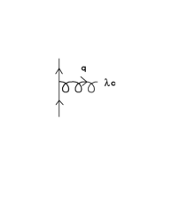
Figure 11: The rho–nucleon vertex from Eq. (98). Here $q^{\mu}=p_{i}^{\mu}-p_{f}^{\mu}$.

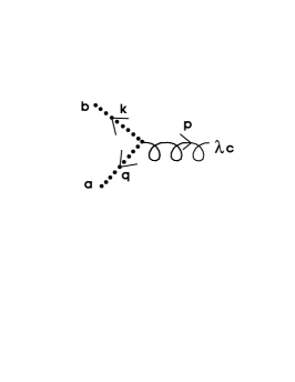
Figure 12: The rho–pi–pi vertex from Eq. (99). Here $p^{\mu}+k^{\mu}+q^{\mu}=0$.

Next one can calculate the total additional Noether currents using the traditional definition [see Ref. Ser86 , Eq. (7.5)]:

$${\delta}{\cal J}^{\lambda}_{a}=-{{\partial({\cal L}_{\rho})}\over{\partial({\partial}_{\lambda}\xi)}}{{\partial(\delta\xi)}\over{\partial{\epsilon}^{a}}}-{{\partial({\cal L}_{\rho})}\over{\partial({\partial}_{\lambda}{\xi}^{{\dagger}})}}{{\partial(\delta{\xi}^{{\dagger}})}\over{\partial{\epsilon}^{a}}}-{{\partial({\cal L}_{\rho})}\over{\partial({\partial}_{\lambda}{\rho}^{d}_{\mu})}}{{\partial(\delta{\rho}_{\mu}^{d})}\over{\partial{\epsilon}^{a}}}\equiv{\delta}_{{\xi}+{\xi}^{{\dagger}}}{\cal J}^{\lambda}_{a}+{\delta}_{\rho}{\cal J}^{\lambda}_{a}\ ,$$ (100)

where the $\bm{\epsilon}$ are global infinitesimal parameters ($\bm{\alpha}$ or $\bm{\beta}$). The partial derivative of the lagrangian (65) with respect to the $\rho$ field is

$${{\partial({\cal L}_{\rho})}\over{\partial({\partial}_{\mu}{\rho}^{d}_{\lambda})}}=-{{f_{\rho}g_{\rho}}\over{4M}}\,{\overline{N\mkern 3.0mu}\mkern-3.0mu}{}\mkern 2.0mu{\sigma}^{\mu\lambda}{\tau}^{d}N-{\rm Tr}({\tau}^{d}{\rho}^{\mu\lambda})\\ -g_{\rho\pi\pi}\,{{2f_{\pi}^{2}}\over{m_{\rho}^{2}}}\,{\rm Tr}({\tau}^{d}{v}^{\mu\lambda})\ .$$

Thus, to lowest order in the meson fields, the part of the Noether vector current due to differentiating with respect to the $\rho$ field is

$${\delta}_{\rho}V^{\lambda}_{a}=-{\epsilon}^{abc}{\rho}^{b}_{\nu}\left\{{{f_{\rho}g_{\rho}}\over{4M}}\,{\overline{N\mkern 3.0mu}\mkern-3.0mu}{}\mkern 2.0mu{\sigma}^{\lambda\nu}{\tau}^{c}N+{\partial}^{[\lambda}\,{\rho}^{\nu]}_{c}+O({\pi}^{2})\right\}\ ,$$ (101)

where the brackets around the superscripts signify the antisymmetric combination, and repeated isospin indices are summed over, regardless of their (vertical) position. The corresponding axial current is

$${\delta}_{\rho}A^{\lambda}_{a}={{1}\over{2f_{\pi}}}{\epsilon}^{abc}{\epsilon}^{cdf}{\pi}^{b}{\rho}^{d}_{\nu}\left\{{{f_{\rho}g_{\rho}}\over{4M}}\,{\overline{N\mkern 3.0mu}\mkern-3.0mu}{}\mkern 2.0mu{\sigma}^{\lambda\nu}{\tau}^{f}N+{\partial}^{[\lambda}\,{\rho}^{\nu]}_{f}+O({\pi}^{2})\right\}\ .$$ (102)

The canonical momentum for the $\rho$ field is, to lowest order,

$$(P_{\rho})^{\lambda\,f}\equiv{{\partial({\cal L}_{\rho})}\over{\partial({\partial}_{0}{\rho}^{f}_{\lambda})}}=-{{f_{\rho}g_{\rho}}\over{4M}}\,{\overline{N\mkern 3.0mu}\mkern-3.0mu}{}\mkern 2.0mu{\sigma}^{0\lambda}{\tau}^{f}N-{\partial}^{[0}_{\vphantom{f}}\,{\rho}^{\lambda]}_{f}+O({\pi}^{2})\ ,$$ (103)

which implies

$${\delta}_{\rho}V^{a0}={\epsilon}^{abc}{\rho}^{b}_{\nu}(P_{\rho})^{\nu\,c}$$ (104)

and

$${\delta}_{\rho}A^{a0}=-{{1}\over{2f_{\pi}}}\,{\epsilon}^{abc}{\epsilon}^{cdf}{\pi}^{b}{\rho}^{d}_{\nu}(P_{\rho})^{\nu\,f}\ .$$ (105)

Consider now a derivative of the lagrangian (65) with respect to the $\xi$ field. To lowest order in the fields, the corresponding axial current is

$${\delta}_{{\xi}+{\xi}^{{\dagger}}}A^{\lambda}_{a}\approx{}-{{1}\over{2f_{\pi}}}\,{{f_{\rho}g_{\rho}}\over{4M}}\,{\epsilon}^{abc}{\epsilon}^{cdf}{\pi}^{b}{\rho}^{d}_{\nu}\,{\overline{N\mkern 3.0mu}\mkern-3.0mu}{}\mkern 2.0mu{\sigma}^{\lambda\nu}{\tau}^{f}N+g_{\rho\pi\pi}\,{{2f_{\pi}}\over{m_{\rho}^{2}}}\,{\epsilon}^{abc}\,{\partial}_{\nu}{\pi}^{b}{\partial}^{[\lambda}\,{\rho}^{\nu]}_{c}\ ,$$ (106)

and thus the total additional axial current is

$${\delta}A^{\lambda}_{a}=g_{\rho\pi\pi}\,{{2f_{\pi}}\over{m_{\rho}^{2}}}\,{\epsilon}^{abc}\,{\partial}_{\nu}{\pi}^{b}\,{\partial}^{[\lambda}\,{\rho}^{\nu]}_{c}+O(\rho^{2}\pi,\,\rho\pi^{3})\ .$$ (107)

It is now clear why we kept the $\rho\pi\pi$ coupling of order $\nu=4$: the $\nu=3$ contributions to the axial-vector current cancel out. The vertex arising from the interaction of this current with the external source can be calculated as in Eqs. (51) and (52), with the result (see Fig. 13)

$${}-i{{2f_{\pi}g_{\rho\pi\pi}}\over{m_{\rho}^{2}}}\,{\epsilon}^{abc}\left({p}^{\mu}{q}^{\lambda}-p\!\cdot\!q\>g^{\mu\lambda}\right)\ .$$ (108)

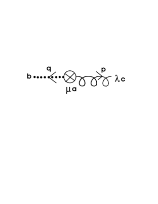
Figure 13: The vertex contribution from the axial current (107), as given in Eq. (108).

Similarly, one finds for the corresponding vector current,

$${\delta}_{\xi+{\xi}^{{\dagger}}}V^{\lambda}_{a}\approx{1\over{2f_{\pi}^{2}}}\,{{f_{\rho}g_{\rho}}\over{4M}}\,{\epsilon}^{abc}{\epsilon}^{cdf}{\epsilon}^{fm\ell}{\pi}^{b}{\pi}^{d}{\rho}^{m}_{\nu}\;{\overline{N\mkern 3.0mu}\mkern-3.0mu}{}\mkern 2.0mu{\sigma}^{\lambda\nu}{\tau}^{\ell}N-{{2g_{\rho\pi\pi}}\over{m_{\rho}^{2}}}\,{\epsilon}^{abc}{\epsilon}^{cdf}{\pi}^{b}\,{\partial}_{\nu}{\pi^{d}}\,\partial^{[\lambda}{\rho}^{\nu]}_{f}\ .\$$ (109)

These terms are of higher order in the fields, namely $O(\rho{\pi}^{2})$, than those in Eq. (101) and thus are not considered in the sequel.

VI.2 The corresponding chiral algebra

The terms in the additional $\rho$ meson lagrangian (65) that involve derivatives of fields can be written, to lowest order in the pion field, as

$$\delta{\cal L}_{\partial} \approx -{{f_{\rho}g_{\rho}}\over{4M}}\,{\partial}_{\mu}{\rho}_{\nu}^{a}\,{\overline{N\mkern 3.0mu}\mkern-3.0mu}{}\mkern 2.0mu{\sigma}^{\mu\nu}{\tau}^{a}N+{{1}\over{2f_{\pi}^{2}}}\,{{f_{\rho}g_{\rho}}\over{4M}}\,{\epsilon}^{abc}{\epsilon}^{cdf}{\pi}^{a}\,{\partial}_{\mu}{\pi}^{b}{\rho}_{\nu}^{d}\,{\overline{N\mkern 3.0mu}\mkern-3.0mu}{}\mkern 2.0mu{\sigma}^{\mu\nu}{\tau}^{f}N$$ (110)

$$\quad{}-{{1}\over{2}}\,{\partial}_{\mu}{\rho}_{\nu}^{a}\,{\partial}^{[\mu}{\rho}^{\nu]}_{a}-{{\overline{g\mkern 2.0mu}\mkern-2.0mu}{}}_{\rho}\,{\epsilon}^{abc}{\rho}_{\mu}^{a}\,{\rho}_{\nu}^{b}\,{\partial}^{\mu}{\rho}^{\nu}_{c}-{{g_{\rho\pi\pi}}\over{m_{\rho}^{2}}}\,{\epsilon}^{abc}\,{\partial}_{\mu}{\pi}^{a}{\partial}_{\nu}{\pi}^{b}{\partial}^{[\mu}{\rho}^{\nu]}_{c}\ .$$

Hence

$${{\partial(\delta{\cal L}_{\partial})\over{\partial({\partial}_{\lambda}{\pi}^{a})}}}=-{{1}\over{2f_{\pi}^{2}}}\,{{f_{\rho}g_{\rho}}\over{4M}}\,{\epsilon}^{abc}{\epsilon}^{cdf}{\pi}^{b}{\rho}_{\nu}^{d}\,{\overline{N\mkern 3.0mu}\mkern-3.0mu}{}\mkern 2.0mu{\sigma}^{\lambda\nu}{\tau}^{f}N-{{2g_{\rho\pi\pi}}\over{m_{\rho}^{2}}}\,{\epsilon}^{abc}\,{\partial}_{\nu}{\pi}^{b}\,{\partial}^{[\lambda}\,{\rho}^{\nu]}_{c}\ .$$ (111)

Moreover, again to lowest order,

$${\delta}_{\xi+{\xi}^{{\dagger}}}A^{a\lambda}=-f_{\pi}\>{{\partial(\delta{\cal L}_{\partial})\over{\partial({\partial}_{\lambda}{\pi}^{a})}}}$$ (112)

and

$${\delta}_{\xi+{\xi}^{{\dagger}}}A^{a0}=-f_{\pi}\>\delta P_{\pi}^{a}\ .$$ (113)

This term has the same form as the pionic contribution in Eq. (28), when the latter is expanded to leading order in the pion field. Thus, when the full axial-vector charge density is expressed in terms of the total pion canonical momentum, the pion terms look the same as they did before. This implies that the axial-vector piece ${\delta}_{\xi+{\xi}^{{\dagger}}}A^{a0}$ does not influence the chiral charge algebra. One also recalls that the vector current ${\delta}_{\xi+{\xi}^{{\dagger}}}V^{a\lambda}$ in Eq. (109) is of higher order in the meson fields and does not influence the chiral charge algebra to the order that we consider here.

The only remaining pieces to consider for the proof of the chiral charge algebra are ${\delta}_{\rho}V^{a0}$ and ${\delta}_{\rho}A^{a0}$. We can write the total charge densities as

$$V^{a0}_{\rm tot}\equiv V^{a0}+{\delta}_{\rho}V^{a0}\ ,$$ (114)

$$A^{a0}_{\rm tot}\equiv A^{a0}+{\delta}_{\rho}A^{a0}\ .$$ (115)

Here $V^{a0}$ and $A^{a0}$ are taken from Eqs. (76) and (77) expanded to lowest order in the meson fields.

First, consider the commutator of the total axial charge densities

$$[A^{a0}_{\rm tot},\>{A^{b0}_{\rm tot}}]=[A^{a0},\>A^{b0}]+[A^{a0},\>{\delta}_{\rho}A^{b0}]+[{\delta}_{\rho}A^{a0},\>A^{b0}]+[{\delta}_{\rho}A^{a0},\>{\delta}_{\rho}A^{b0}]\ .$$ (116)

The first commutator in this expression is known:

$$[A^{a0},\>A^{b0}]\propto i{\epsilon}^{abc}V^{c0}\ ,$$ (117)

while the second and third terms are equal to

$$[A^{a0},\>{\delta}_{\rho}A^{b0}]\approx-{{1}\over{2f_{\pi}}}\,{\epsilon}^{b\ell c}{\epsilon}^{cdf}(-f_{\pi}){\rho}^{d}_{\nu}(P_{\rho})^{\nu\,f}\left[P_{\pi}^{a},\>{\pi}^{\ell}\right]\ .$$ (118)

Thus, to lowest order in the meson fields,

$$[A^{a0},\>{\delta}_{\rho}A^{b0}]+[{\delta}_{\rho}A^{a0},\>A^{b0}]\propto i{\epsilon}^{abc}{\epsilon}^{cdf}{\rho}^{d}_{\nu}(P_{\rho})^{\nu\,f}=i{\epsilon}^{abc}{\delta}_{\rho}V^{c0}\ .$$ (119)

The final commutator is of third order in the meson fields,

$$[{\delta}_{\rho}A^{a0},\>{\delta}_{\rho}A^{b0}]\propto O(\rho{\pi}^{2})\ ,$$ (120)

and does not contribute to the charge algebra to the order we are working. By combining the results in Eqs. (117) and (119), we find that the first relation of the charge algebra holds in the presence of the additional terms in the lagrangian:

$$[(Q^{a}_{5})_{\rm tot},\>(Q^{b}_{5})_{\rm tot}]=i{\epsilon}^{abc}\,Q^{c}_{\rm tot}\ .$$ (121)

Next, consider the commutator of vector charge densities

$$[V^{a0}_{\rm tot},\>{V^{b0}_{\rm tot}}]=[V^{a0},\>V^{b0}]+[V^{a0},\>{\delta}_{\rho}V^{b0}]+[{\delta}_{\rho}V^{a0},\>V^{b0}]+[{\delta}_{\rho}V^{a0},\>{\delta}_{\rho}V^{b0}]\ .$$ (122)

As before, the first commutator is known:

$$[V^{a0},\>V^{b0}]\propto i{\epsilon}^{abc}V^{c0}\ ,$$ (123)

while the second and third commutators vanish because pion, nucleon, and rho factors commute with each other. The final commutator can be written as

$$[{\delta}_{\rho}V^{a0},\>{\delta}_{\rho}V^{b0}]\approx{\epsilon}^{adc}{\epsilon}^{bmn}\left[{\rho}^{d}_{\nu}(P_{\rho})^{\nu\,c},\;{\rho}^{m}_{\mu}(P_{\rho})^{\mu\,n}\right]\ ,$$ (124)

or, after some algebraic manipulation,

$$[{\delta}_{\rho}V^{a0},\>{\delta}_{\rho}V^{b0}]\propto i{\epsilon}^{abc}{\epsilon}^{cdn}{\rho}^{d}_{\nu}(P_{\rho})^{\nu\,n}=i{\epsilon}^{abc}{\delta}_{\rho}V^{c0}\ .$$ (125)

Thus the second relation of the chiral algebra,

$$[Q^{a}_{\rm tot},\>Q^{b}_{\rm tot}]=i{\epsilon}^{abc}\,Q^{c}_{\rm tot}\ ,$$ (126)

also holds.

Finally, consider the commutator of axial and vector charge densities:

$$[A^{a0}_{\rm tot},\>{V^{b0}_{\rm tot}}]=[A^{a0},\>V^{b0}]+[A^{a0},\>{\delta}_{\rho}V^{b0}]+[{\delta}_{\rho}A^{a0},\>V^{b0}]+[{\delta}_{\rho}A^{a0},\>{\delta}_{\rho}V^{b0}]\ .$$ (127)

The first commutator is known:

$$[A^{a0},\>V^{b0}]\propto i{\epsilon}^{abc}A^{c0}\ .$$ (128)

The second commutator vanishes because pion and nucleon fields commute with rho fields. The third commutator can be written as

$$[{\delta}_{\rho}A^{a0},\>V^{b0}]\propto-{i\over{2f_{\pi}}}\,{\epsilon}^{a\ell c}{\epsilon}^{cdf}{\epsilon}^{bn\ell}{\pi}^{n}{\rho}^{d}_{\nu}(P_{\rho})^{\nu\,f}\ .$$ (129)

The final commutator is

$$[{\delta}_{\rho}A^{a0},\>{\delta}_{\rho}V^{b0}]\approx-{1\over{2f_{\pi}}}\,{\epsilon}^{af\ell}{\epsilon}^{\ell dc}{\epsilon}^{bmn}{\pi}^{f}\left[{\rho}^{d}_{\nu}(P_{\rho})^{\nu\,c},\;{\rho}^{m}_{\mu}(P_{\rho})^{\mu\,n}\right]\ ,$$ (130)

which, after some algebra, becomes

$$[{\delta}_{\rho}A^{a0},\>{\delta}_{\rho}V^{b0}]\propto-{i\over{2f_{\pi}}}\,{\epsilon}^{an\ell}{\epsilon}^{\ell bc}{\epsilon}^{cdf}{\pi}^{n}{\rho}^{d}_{\nu}(P_{\rho})^{\nu\,f}\ .$$ (131)

By using the relation

$${\epsilon}^{a\ell c}{\epsilon}^{bn\ell}+{\epsilon}^{an\ell}{\epsilon}^{\ell bc}={\epsilon}^{abm}{\epsilon}^{mnc}\ ,\quad$$ (132)

one can show that the sum of the third and fourth commutators is

$$[{\delta}_{\rho}A^{a0},\>V^{b0}]+[{\delta}_{\rho}A^{a0},\>{\delta}_{\rho}V^{b0}]\propto i{\epsilon}^{abc}\left(-{{1}\over{2f_{\pi}}}\,{\epsilon}^{cnp}{\epsilon}^{pdf}{\pi}^{n}{\rho}^{d}_{\nu}(P_{\rho})^{\nu\,f}\right)\ .$$ (133)

The term in the parentheses is just ${\delta}_{\rho}A^{c0}$. Thus

$$[(Q^{a}_{5})_{\rm tot},\>Q^{b}_{\rm tot}]=i{\epsilon}^{abc}\,(Q^{c}_{5})_{\rm tot}\ ,$$ (134)

and therefore all of the relations constituting the chiral charge algebra hold in the presence of the included extra terms in the QHD lagrangian.

VI.3 Two-nucleon, axial-current amplitudes

The two-body, axial-current amplitudes involving the rho meson are given by the diagrams in Fig. 14.

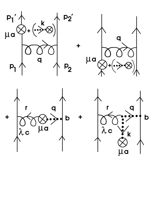
Figure 14: Two-nucleon, axial-current amplitudes containing rho meson exchange. The notation in the first two diagrams implies that the external source can couple to the nucleon line in two ways, as in Fig. 6.

The diagrams in the first row of this figure originate from the terms of order $\nu\leq 3$ in the $\rho$ meson lagrangian (65), while the diagrams in the second row correspond to the $\nu=4$ terms. Thus

$$M^{a\mu}(2) \approx ig_{A}\,g_{\rho}^{2}\;\frac{(g_{\lambda\alpha}-q_{\lambda}q_{\alpha}/m_{\rho}^{2})}{q^{2}-m_{\rho}^{2}}\left(g^{\mu}_{\phantom{\mu}\sigma}-\frac{k^{\mu}k_{\sigma}}{k^{2}-m_{\pi}^{2}}\right)$$ (135)

$$\qquad{}\times\bar{u}(p_{2}^{\prime})\left(\gamma^{\alpha}-\frac{f_{\rho}}{2M}\,iq_{\beta}\sigma^{\beta\alpha}\right)\frac{\tau^{c}}{2}\,u(p_{2})$$

$$\qquad{}\times\bar{u}(p_{1}^{\prime})\left\{\gamma_{5}\gamma^{\sigma}\frac{1}{(\not\!p_{1}-\mbox{{$q$}{$\!\!\!/\,$}})-M}\left(\gamma^{\lambda}+\frac{f_{\rho}}{2M}\,iq_{\nu}\sigma^{\nu\lambda}\right)\frac{\tau^{a}}{2}\frac{\tau^{c}}{2}\right.$$

$$\qquad\qquad\qquad\quad\left.{}+\left(\gamma^{\lambda}+\frac{f_{\rho}}{2M}\,iq_{\nu}\sigma^{\nu\lambda}\right)\frac{1}{(\not\!p^{\mkern 2.0mu\prime}_{1}+\mbox{{$q$}{$\!\!\!/\,$}})-M}\,\gamma_{5}\gamma^{\sigma}\,\frac{\tau^{c}}{2}\frac{\tau^{a}}{2}\right\}u(p_{1})$$

$$\quad{}+\frac{2g_{A}\,g_{\rho}\,g_{\rho\pi\pi}}{m_{\rho}^{2}}\,\epsilon^{abc}\,\bar{u}(p_{2}^{\prime})\gamma_{5}\,\mbox{{$q$}{$\!\!\!/\,$}}\frac{\tau^{b}}{2}\,u(p_{2})\;\bar{u}(p_{1}^{\prime})\left(\gamma^{\lambda}-\frac{f_{\rho}}{2M}\,ir_{\nu}\sigma^{\nu\lambda}\right)\frac{\tau^{c}}{2}\,u(p_{1})$$

$$\qquad{}\times\frac{(g_{\lambda\alpha}-r_{\lambda}r_{\alpha}/m_{\rho}^{2})}{r^{2}-m_{\rho}^{2}}\,\frac{1}{q^{2}-m_{\pi}^{2}}$$

$$\qquad{}\times\left\{r^{\mu}q^{\alpha}-(r\cdot q)g^{\mu\alpha}+\frac{k^{\mu}}{k^{2}-m_{\pi}^{2}}\,[(q\cdot r)k^{\alpha}-(k\cdot r)q^{\alpha}]\right\}$$

$$\quad{}+(\mathrm{direct})_{2}+{\mathrm{\ cross\ terms.}}$$

The terms proportional to $g_{\rho}^{2}$ satisfy PCAC by themselves, precisely as in the nonlinear realization of the Sigma model. The terms proportional to $g_{\rho\pi\pi}$ also satisfy PCAC separately because

$$k_{\mu}\left\{r^{\mu}q^{\alpha}-(r\cdot q)g^{\mu\alpha}+\frac{k^{\mu}}{k^{2}-m_{\pi}^{2}}\,[(q\cdot r)k^{\alpha}-(k\cdot r)q^{\alpha}]\right\}\lower 8.1805pt\vbox{\hbox{$\ \buildrel{\hbox{\Large\rightarrowfill}}\over{\scriptstyle{m_{\pi}\,\rightarrow\,0}}\ $}}\,0\ .$$ (136)

One can identify the corresponding additional AXC from these amplitudes.

VII Contributions from sigma and omega mesons

Now one can easily add the $\sigma$ and $\omega$ contributions in the present EFT. The corresponding lowest-order interaction terms can be deduced from the full lagrangian (2):

$${\cal L}^{\rm int}_{\sigma}\approx g_{s}\phi\,{\overline{N\mkern 3.0mu}\mkern-3.0mu}{}\mkern 2.0muN+{\eta}_{\rho}{{g_{s}}m^{2}_{\rho}\over M}\,\phi\,{\rm Tr}({\rho}_{\mu}{\rho}^{\mu})-{{\kappa_{3}}\over{3!}}\,{{g_{s}}m^{2}_{s}\over M}\,{\phi}^{3}\ .$$ (137)

The final two terms involve interactions that are of higher order in the meson fields than we consider here for the two-body axial current, so we will not discuss them further. Similarly,

$${\cal L}^{\rm int}_{\omega}\approx-g_{v}V_{\mu}\,{\overline{N\mkern 3.0mu}\mkern-3.0mu}{}\mkern 2.0mu{\gamma}^{\mu}N-{{f_{v}g_{v}}\over{4M}}\,{\partial}_{\,[\mu}V_{\nu]}\mkern 2.0mu{\overline{N\mkern 3.0mu}\mkern-3.0mu}{}\mkern 2.0mu{\sigma}^{\mu\nu}N+{1\over 2}\,{\eta}_{1}{{g_{s}}m^{2}_{v}\over M}\,\phi V_{\mu}V^{\mu}\ .$$ (138)

Again, the final term above is of higher order in the meson fields and does not contribute here.

We obtain the following new strong-interaction vertices that look exactly like the one in Fig. 2, but with the pion line replaced by sigma and omega lines, respectively (see Ref. Ser86 , Fig. 29):

$$ig_{s}\ ,$$ (139)

$$-ig_{v}\left({\gamma}^{\lambda}+{{f_{v}}\over{2M}}\,iq_{\nu}{\sigma}^{\nu\lambda}\right)\ .\\$$ (140)

Both $\sigma$ and $\omega$ mesons are chiral scalars and thus do not contribute to the Noether axial-vector current.

The amplitudes for the two-body, axial-vector currents involving $\sigma$ and $\omega$ meson exchange are represented by diagrams analogous to those in the first row of Fig. 14. They are given by the first term in Eq. (135), with the appropriate meson propagator substituted for the $\rho$ propagator, and with the expression (98) for the rho–nucleon vertex replaced by the sigma–nucleon vertex (139) or the omega–nucleon vertex (140), respectively.

VIII Summary

In this work, we compute the axial-vector current based on a recently proposed hadronic lagrangian with a nonlinear realization of chiral symmetry Fur97 . The effective lagrangian provides a systematic framework for calculating both nuclear exchange currents and nuclear wave functions. The lagrangian is truncated by working to a fixed order in the parameter $\nu$, which essentially counts powers of ratios of particle momenta to the nucleon mass $M$ or of mean meson fields to the nucleon mass Fur97 ; Rus97 . Practically speaking, in the nuclear many-body problem, the expansion is in powers of $k_{\mathrm{F}}/M$, where $k_{\mathrm{F}}$ is the Fermi wavenumber at equilibrium nuclear density; this ratio provides a small parameter for ordinary nuclei and for electroweak processes at modest momentum transfers.

The present framework has several advantages: First, because of the nonlinear realization of the chiral symmetry, the axial coupling constant $g_{A}\!\approx\!1.26$ appears naturally as a parameter in the lagrangian. Second, the explicit enforcement of the symmetry ensures that the axial current is conserved in the chiral limit (and that PCAC holds for finite pion mass), and that the familiar $SU(2)_{L}\times SU(2)_{R}$ chiral algebra is satisfied by the vector and axial-vector charges. The symmetry also implies that there will be axial-vector exchange currents (AXC) involving nonlinear meson couplings. Third, since the same degrees of freedom are used to describe the axial-vector current and the nuclear dynamics, the parameters of the theory can be calibrated using empirical nuclear and hadronic properties (or two-nucleon bound-state and scattering data), together with pion–nucleon scattering observables. Thus there are no unknown constants in the axial-current amplitudes. To our knowledge, these desirable properties have not been included simultaneously in earlier models of the AXC.

The axial currents are derived here by keeping all relevant terms in the lagrangian through order $\nu=3$ (and $\nu=4$ in the $\rho$ meson case). In the chiral limit, the correct chiral charge algebra is proved explicitly to all orders in the pion field for terms involving pions and nucleons, and to lowest order in the pion field for terms involving pions, nucleons, and rho mesons. For finite pion mass, it is also shown that PCAC holds for the one- and two-body axial-current amplitudes, as well as for the amplitude for pion production on a single nucleon. The AXC can be deduced from the two-nucleon amplitudes, although we do not derive them in this paper. [We do, however, compute the leading (nonrelativistic) correction to the axial charge density in Eq. (61).]

Since our analysis of the axial-vector current in the nuclear many-body problem is performed by splitting our EFT lagrangian into numerous pieces, it is useful to summarize here our most important results and expressions. The complete vector and axial-vector currents are given in Eqs. (25) and (26), plus (38) and (39) [or (40) and (41)], plus (69) and (70) [or (LABEL:eq:vector-3-pi) and (75)], plus (101) and (107). Thus, for example, the complete currents are

$$V_{\mathrm{tot}}^{a\mu} = -i\,{{f_{\pi}^{2}}\over 4}\,{\rm Tr}\left\{{\tau}^{a}\left(U{\partial}^{\mu}U^{{\dagger}}+U^{{\dagger}}{\partial}^{\mu}U\right)\right\}$$ (141)

$$\quad{}+{{1}\over{4}}\,{\overline{N\mkern 3.0mu}\mkern-3.0mu}{}\mkern 2.0mu{\gamma}^{\mu}\left[{\xi}{\tau}^{a}{\xi}^{{\dagger}}+{\xi}^{{\dagger}}{\tau}^{a}{\xi}\right]N+{{1}\over{4}}\,g_{A}{\overline{N\mkern 3.0mu}\mkern-3.0mu}{}\mkern 2.0mu{\gamma}^{\mu}{\gamma}_{5}\left[{\xi}{\tau}^{a}{\xi}^{{\dagger}}-{\xi}^{{\dagger}}{\tau}^{a}{\xi}\right]N$$

$$\quad{}-{{i{\kappa}_{\pi}}\over{2M}}\>{\overline{N\mkern 3.0mu}\mkern-3.0mu}{}\mkern 2.0mu{\sigma}^{\mu\nu}\left[{\xi}^{{\dagger}}{\tau}^{a}\xi-\xi{\tau}^{a}{\xi}^{{\dagger}},\>a_{\nu}\right]N-{{2{\beta}_{\pi}}\over{M}}\>{\overline{N\mkern 3.0mu}\mkern-3.0mu}{}\mkern 2.0muN\>{\rm Tr}\left[({\xi}^{{\dagger}}{\tau}^{a}\xi-\xi{\tau}^{a}{\xi}^{{\dagger}})\>a^{\mu}\right]$$

$$\quad{}-{\epsilon}^{abc}{\rho}^{b}_{\nu}\left\{{{f_{\rho}g_{\rho}}\over{4M}}\,{\overline{N\mkern 3.0mu}\mkern-3.0mu}{}\mkern 2.0mu{\sigma}^{\mu\nu}{\tau}^{c}N+{\partial}^{[\mu}\,{\rho}^{\nu]}_{c}+O({\pi}^{2})\right\}$$

and

$$A_{\mathrm{tot}}^{a\mu} = -i\,{{f_{\pi}^{2}}\over 4}\,{\rm Tr}\left\{{\tau}^{a}\left(U{\partial}^{\mu}U^{{\dagger}}-U^{{\dagger}}{\partial}^{\mu}U\right)\right\}$$ (142)

$$\quad{}-{{1}\over{4}}\,{\overline{N\mkern 3.0mu}\mkern-3.0mu}{}\mkern 2.0mu{\gamma}^{\mu}\left[{\xi}{\tau}^{a}{\xi}^{{\dagger}}-{\xi}^{{\dagger}}{\tau}^{a}{\xi}\right]N-{{1}\over{4}}\,g_{A}{\overline{N\mkern 3.0mu}\mkern-3.0mu}{}\mkern 2.0mu{\gamma}^{\mu}{\gamma}_{5}\left[{\xi}{\tau}^{a}{\xi}^{{\dagger}}+{\xi}^{{\dagger}}{\tau}^{a}{\xi}\right]N$$

$$\quad{}-{{i{\kappa}_{\pi}}\over{2M}}\>{\overline{N\mkern 3.0mu}\mkern-3.0mu}{}\mkern 2.0mu{\sigma}^{\mu\nu}\left[{\xi}^{{\dagger}}{\tau}^{a}\xi+\xi{\tau}^{a}{\xi}^{{\dagger}},\>a_{\nu}\right]N-{{2{\beta}_{\pi}}\over{M}}\>{\overline{N\mkern 3.0mu}\mkern-3.0mu}{}\mkern 2.0muN\>{\rm Tr}\left[({\xi}^{{\dagger}}{\tau}^{a}\xi+\xi{\tau}^{a}{\xi}^{{\dagger}})\>a^{\mu}\right]$$

$$\quad{}+\left\{g_{\rho\pi\pi}\,{{2f_{\pi}}\over{m_{\rho}^{2}}}\,{\epsilon}^{abc}\,{\partial}_{\nu}{\pi}^{b}\,{\partial}^{[\mu}\,{\rho}^{\nu]}_{c}+O(\rho^{2}\pi,\,\rho\pi^{3})\right\}\ .$$

We also derived expressions for the following amplitudes: the scattering of a nucleon by an external source [Eqs. (54), (83), and (89)], one-pion production by an external source [Eqs. (57), (84), and (90)], and nucleon–nucleon scattering in the presence of an external source [Eqs. (59), (86), (92), and (135)]. All of these results were evaluated at the “tree” level, with no pion loops. This is because we computed the scattering matrices to lowest order in the external source $S^{\mathrm{ext}}_{a\mu}$, and we expanded the interaction lagrangian to leading orders in the pion field. As noted above, since our expansion proceeds in powers of pion momenta (or $m_{\pi}$) relative to the nucleon mass $M$ (or a similar “heavy” mass scale), these tree-level expressions are valid for modest external pion momenta and momentum transfers between nucleons. Our results become exact in the soft-pion limit (with $m_{\pi}=0$).

At order $\nu=2$, our EFT lagrangian generates familiar pion-exchange contributions to the AXC. These are the same as those calculated by Kubodera, Delorme, and Rho Kub78 in the current-algebra approach. We reiterate the cause of the difficulty in Ref. Ana98 , and how that problem is resolved by the EFT lagrangian (2): in a linear realization of the $SU(2)_{L}\times SU(2)_{R}$ chiral symmetry, the nucleon axial-vector coupling $g_{A}$ is constrained to be unity. Changing this coupling “by hand” is equivalent to rescaling the fields in the theory and leads to a chiral charge algebra that is incorrect. In contrast, in a nonlinear realization of the symmetry, $g_{A}$ becomes a free parameter, which allows the Goldberger–Treiman relation, PCAC, and the correct chiral charge algebra to be satisfied simultaneously. This is explicit evidence that chiral symmetry is realized nonlinearly in low-energy QCD.

In future work, we will show that the dominant contributions to the axial-vector current come from one- and two-body amplitudes involving pion exchange and are thus model independent Rho91 . The relevant set of $\nu=3$ AXC will be written in covariant form for use with relativistic, mean-field Dirac wave functions, and the dominant $\nu=3$ terms will also be given in nonrelativistic form for use with more traditional (e.g., harmonic oscillator) nucleon wave functions. We now have the effective lagrangian and corresponding Noether currents, and the problem is therefore well defined; however, as emphasized in Refs. Dmi98 ; Ana98 , any application to the many-body problem must proceed consistently in terms of wave functions, the interactions that determine those wave functions, and the current operators to be used within that framework.

We also plan to derive the meson-exchange corrections to the electromagnetic current that are implied by this effective lagrangian Fur97 . These meson-exchange corrections can then be used to compute selected electroweak processes in nuclei. This will allow, for example, for an investigation of the following interesting issue: It is known that calibrating the relevant parameters to nuclear properties using mean-field nuclear wave functions corresponds to a density-functional approach Ser97 ; Fur97 ; Ser02 . In this approach, bulk and single-particle nuclear observables are used to define a set of quasiparticle, single-nucleon wave functions, which implies that exchange and correlation corrections are (approximately) included implicitly in the parameters. Within this quasiparticle, single-nucleon framework, we expect that the PCAC relations derived here will remain valid. In the calculation of exchange-current amplitudes, however, one samples two-nucleon wave functions inside the nucleus. It remains to be seen whether the calibration procedure described above leads to realistic results for two-body, exchange-current matrix elements, or if some more complicated calibration procedure (that also includes two-body observables) must be used.

References

- (1) R. Machleidt, Adv. Nucl. Phys. 19, 189 (1989).
- (2) R. Machleidt, Phys. Rev. C 63, 024001 (2001).
- (3) J. D. Walecka, Theoretical Nuclear and Subnuclear Physics (Oxford Univ. Press, New York, 1995).
- (4) B. D. Serot and J. D. Walecka, Adv. Nucl. Phys. 16, 1 (1986).
- (5) B. D. Serot and J. D. Walecka, Int. J. Mod. Phys. E 6, 515 (1997).
- (6) S. Weinberg, Physica 96A, 327 (1979).
- (7) S. Weinberg, The Quantum Theory of Fields, Vol. I: Foundations (Cambridge Univ. Press, Cambridge, 1995).
- (8) R. J. Furnstahl, H.-W. Hammer, and N. Tirfessa, Nucl. Phys. A689, 846 (2001).
- (9) J. D. Walecka, Ann. Phys. (N.Y.) 83, 491 (1974).
- (10) R. J. Furnstahl and B. D. Serot, Comments Nucl. Part. Phys. 2, A23 (2000).
- (11) B. D. Serot and J. D. Walecka, in 150 Years of Quantum Many-Body Theory, edited by R. F. Bishop, K. A. Gernoth, and N. R. Walet (World Scientific, Singapore, 2001), p. 203.
- (12) J. Dubach, J. H. Koch, and T. W. Donnelly, Nucl. Phys. A271, 279 (1976).
- (13) Mesons in Nuclei, edited by M. Rho and D. Wilkinson (North-Holland, Amsterdam, 1979).
- (14) D. O. Riska, Phys. Rep. 181, 207 (1989).
- (15) V. Dmitrašinović and T. Sato, Phys. Rev. C 58, 1937 (1998).
- (16) K. Kubodera, J. Delorme, and M. Rho, Phys. Rev. Lett. 40, 755 (1978).
- (17) P. G. Blunden and D. O. Riska, Nucl. Phys. A536, 697 (1992).
- (18) M. Kirchbach, D. O. Riska, and K. Tsushima, Nucl. Phys. A542, 616 (1992).
- (19) M. Kirchbach and D. O. Riska, Nucl. Phys. A578, 511 (1994).
- (20) D. O. Riska, Phys. Rep. 242, 345 (1994).
- (21) E. Ivanov and E. Truhlík, Nucl. Phys. A316, 437 (1979).
- (22) I. S. Towner, Nucl. Phys. A542, 631 (1992).
- (23) J. G. Congleton and E. Truhlík, Phys. Rev. C 53, 956 (1996).
- (24) J. Smejkal, E. Truhlík, and H. Goeller, Nucl. Phys. A624, 655 (1997).
- (25) M. Rho, Phys. Rev. Lett. 66, 1275 (1991).
- (26) T.-S. Park, D.-P. Min, and M. Rho, Phys. Rep. 233, 341 (1993).
- (27) T.-S. Park, I. S. Towner, and K. Kubodera, Nucl. Phys. A579, 381 (1994).
- (28) T.-S. Park, D.-P. Min, and M. Rho, Nucl. Phys. A596, 515 (1996).
- (29) T.-S. H. Lee and D. O. Riska, Phys. Rev. Lett. 70, 2237 (1993).
- (30) B. D. Serot and J. D. Walecka, Acta Phys. Pol. B 23, 655 (1992).
- (31) R. J. Furnstahl and B. D. Serot, Nucl. Phys. A673, 298 (2000).
- (32) R. J. Furnstahl, B. D. Serot, and H.-B. Tang, Nucl. Phys. A598, 539 (1996).
- (33) R. J. Furnstahl, H.-B. Tang, and B. D. Serot, Phys. Rev. C 52, 1368 (1995).
- (34) R. J. Furnstahl, B. D. Serot, and H.-B. Tang, Nucl. Phys. A615, 441 (1997); A640, 505 (E) (1998).
- (35) E. Epelbaum, W. Glöckle, and Ulf-G. Meißner, Nucl. Phys. A637, 107 (1998).
- (36) E. Epelbaum, W. Glöckle, and Ulf-G. Meißner, Nucl. Phys. A671, 295 (2000).
- (37) E. Epelbaum, Ulf-G. Meißner, W. Glöckle, and C. Elster, Phys. Rev. C 65, 044001 (2002).
- (38) D. R. Entem and R. Machleidt, Phys. Lett. B 524, 93 (2002).
- (39) D. R. Entem and R. Machleidt, Phys. Rev. C 66, 014002 (2002).
- (40) S. M. Ananyan, Phys. Rev. C 57, 2669 (1998).
- (41) J. Schwinger, Ann. Phys. (N.Y.) 2, 407 (1957).
- (42) M. Gell-Mann and M. Lévy, Nuovo Cimento 16, 705 (1960).
- (43) A. K. Kerman and L. D. Miller, in Second High-Energy Heavy Ion Summer Study, Lawrence Berkeley Laboratory report LBL–3675 (1974) (unpublished).
- (44) R. J. Furnstahl and B. D. Serot, Nucl. Phys. A671, 447 (2000).
- (45) H. Georgi, Phys. Lett. B 298, 187 (1993).
- (46) R. M. Dreizler and E. K. U. Gross, Density Functional Theory (Springer-Verlag, Berlin, 1990).
- (47) B. D. Serot, in Advances in Quantum Many-Body Theory, Vol. 5, edited by R. F. Bishop, T. Brandes, K. A. Gernoth, N. R. Walet, and Y. Xian (World Scientific, Singapore, 2002), p. 207.
- (48) F. Gross, J. W. Van Orden, and K. Holinde, Phys. Rev. C 41, R1909 (1990); 45, 2094 (1992).
- (49) J. Gasser, M. E. Sainio, and A. Švarc, Nucl. Phys. B307, 779 (1988).
- (50) P. J. Ellis and H.-B. Tang, Phys. Rev. C 57, 3356 (1998).
- (51) U. van Kolck, Prog. Part. Nucl. Phys. 43, 337 (1999), and references therein.
- (52) S. Coleman, J. Wess, and B. Zumino, Phys. Rev. 177, 2239 (1969).
- (53) C. G. Callan, Jr., S. Coleman, J. Wess, and B. Zumino, Phys. Rev. 177, 2247 (1969).
- (54) C. Itzykson and J.-B. Zuber, Quantum Field Theory (McGraw–Hill, New York, 1980), eq. (1-139).
- (55) F. Mandl and G. Shaw, Quantum Field Theory, revised ed. (Wiley–Interscience, Chichester, UK, 1993), appendixes A and B.
- (56) J. J. Rusnak and R. J. Furnstahl, Nucl. Phys. A627, 495 (1997).
- (57) H.-B. Tang, hep-ph/9607436 (unpublished).