Tensor correlations
in the Unitary Correlation Operator Method

Abstract

We present a unitary correlation operator that explicitly induces into shell model type many-body states short ranged two-body correlations caused by the strong repulsive core and the pronounced tensor part of the nucleon-nucleon interaction. Alternatively an effective Hamiltonian can be defined by applying this unitary correlator to the realistic nucleon-nucleon interaction. The momentum space representation shows that realistic interactions which differ in their short range behaviour are mapped on the same correlated Hamiltonian, indicating a successful provision for the correlations at high momenta. Calculations for $\@@nuc{4}{He}$ using the one- and two-body part of the correlated Hamiltonian compare favorably with exact many-body methods. For heavier nuclei like $\@@nuc{16}{O}$ and $\@@nuc{40}{Ca}$ where exact many-body calculations are not possible we compare our results with other approximations. The correlated single-particle momentum distributions describe the occupation of states above the Fermi momentum. The Unitary Correlation Operator Method (UCOM) can be used in mean-field and shell model configuration spaces that are not able to describe these repulsive and tensor correlations explicitly.

1 Introduction and summary

Quantum Chromo Dynamics (QCD) is the fundamental theory of the strong interaction and the nucleons represent bound systems of quark and gluon degrees of freedom. Nuclear physics in the low energy regime is considered as an effective theory where the center of mass positions, the spins and the isospins of the nucleons are the essential degrees of freedom, whose interaction can be described by a nucleon-nucleon force. In the QCD picture the force between the color neutral nucleons is a residual interaction like the van-der-Waals force between electrically neutral atoms. Therefore it is expected that the nuclear interaction is not a simple local potential but has a rich operator structure in spin and isospin and in many-body systems may also include genuine three- and higher-body forces.

There are attempts to derive the nucleon-nucleon force using Chiral Perturbation Theory [1]. However this approach cannot compete yet with the so-called realistic interactions that reproduce the nucleon-nucleon scattering data and the deuteron properties. The realistic nucleon-nucleon forces are essentially phenomenological. The Bonn interactions [2, 3] are based on meson-exchange that is treated in a relativistic nonlocal fashion. The Argonne interactions [4, 5] on the other hand describe the pion exchange in a local approximation and use a purely phenomenological parameterization of the nuclear interaction at short and medium range.

It is a central challenge of nuclear physics to describe the properties of nuclear many-body systems in terms of such realistic nuclear interactions. However in mean-field and shell-model approaches, typically employed to describe the properties of finite nuclei, realistic interactions cannot be used directly.

Both, relativistic and nonrelativistic mean-field calculations are successful in describing the ground state energies and mass and charge distributions for all nuclei in the nuclear chart but the lightest ones. As the short-range radial and tensor correlations induced by realistic forces cannot be represented by the Slater determinants of the Hartree-Fock method, direct parameterizations of the energy-density or an effective finite range force are used instead.

In shell-model calculations with configuration mixing a two-body Hamiltonian is used in the vector space spanned by the many-body states that represent particle and/or hole configurations in the selected shells. The solution of the energy eigenvalue problem in the high-dimensional many-body space yields detailed information on the spectra of nuclei, the transitions between the states, electromagnetic moments, charge and mass distributions, $\beta$-decay etc. However one has to use an effective interaction in the two-body Hamiltonian. Although one often starts with a G-matrix derived from realistic interactions the two-body matrix elements of the Hamiltonian have to be modified and adjusted to a large set of ground state and excitation energies for an accurate description of the data. This has to be done separately for each region of the nuclear chart.

Only recently it became possible to perform ab initio calculations of the nuclear many-body problem with realistic interactions. In Green’s Function Monte Carlo (GFMC) calculations [6] the exact ground-state wave function is calculated by approximating the many-body Green’s functions in a Monte Carlo approach. The GFMC calculations of light nuclei up to $A=8-10$ with the Argonne interaction demonstrate the necessity of additional three-body forces in order to reproduce the experimental nuclear binding energies and radii as well as the spectra.

Another ab initio approach for nuclei up to $A=12$ is the large-basis no core shell model [7]. All nucleons are treated as active in a large shell-model basis. Despite the large basis it is necessary to treat the short range correlations separately. An effective interaction for the model space is derived in a G-Matrix procedure in two-body approximation.

Ab inito calculations for the doubly magic nuclei $\@@nuc{16}{O}$ and $\@@nuc{40}{Ca}$ are performed with the Correlated Basis Function (CBF) method [8, 9]. Here a perturbation expansion on a complete set of correlated basis functions is performed. The evaluation of expectation values is done in the Fermi Hypernetted Chain (FHNC) method where the Single Operator Chain (SOC) approximation is used.

1.1 Aim

Our aim is to perform ab initio calculations of larger nuclei with realistic interactions in a mean-field or a shell-model many-body approach. To make this possible we introduce a unitary correlation operator ${C}$ that takes care of the short-range radial and tensor correlations. The correlations are not expressed in a certain basis of a model space but are given analytically in terms of operators of relative distance, relative momentum and the spins and isospins of the nucleons. The correlated interaction

$${\hat{H}}={{{C}}}^{{\dagger}}{H}{C}$$ (1)

we obtain by applying the correlation operator to the realistic interaction is therefore not restricted to the model space of a certain many-body theory but can be used for example in a Hartree-Fock calculation as well as in shell-model calculations with configuration mixing. The fact, that the correlations are expressed in a basis-free manner in coordinate space, makes it also easier to understand the physics of the radial and tensor correlations.

Furthermore the unitary correlation operator provides not only a correlated interaction, that can be considered as an effective interaction, but other operators can be correlated as well and the physical implications of the short-range correlations on other observables, for example on the nucleon momentum distributions or the spectroscopic factors, can be evaluated.

The correlated interaction is used successfully with simple shell model and Fermionic Molecular Dynamics [10, 11] Slater determinants. This allows us to perform calculations for all nuclei up to about $A=50$. Although a single Slater determinant as many-body trial state is the most simple ansatz we obtain results very close to those of the quasi-exact methods.

1.2 Procedure

The repulsive core and the strong tensor force of the nuclear interaction induce strong short-range radial and tensor correlations in the nuclear many-body system. These correlations cannot be represented with Slater determinants of single-particle states

$$\big{|}\,{\Psi}\,\big{>}=\mathcal{A}\left\{\big{|}\,{\psi_{1}}\,\big{>}\otimes\ldots\otimes\big{|}\,{\psi_{A}}\,\big{>}\right\}\;,$$ (2)

which are used as many-body states in Hartree-Fock or a shell-model calculations. $\mathcal{A}$ denotes the antisymmetrization operator and $\big{|}\,{\psi_{i}}\,\big{>}$ the single-particle states.

We describe the radial and tensor correlations by a unitary correlation operator that is the product of a radial correlator ${C}_{r}^{\phantom{\dagger}}$ and a tensor correlator ${C}_{\Omega}^{\phantom{\dagger}}$.

$${C}={C}_{\Omega}^{\phantom{\dagger}}{C}_{r}^{\phantom{\dagger}}$$ (3)

The radial correlator ${C}_{r}^{\phantom{\dagger}}$ (described in detail in [12]) shifts a pair of particles in the radial direction away from each other so that they get out of the range of the repulsive core. To perform the radial shifts the generator of the radial correlator uses the radial momentum operator ${p}_{r}$ together with a shift function $s(r)$ that depends on the distance of the two nucleons.

$${C}_{r}^{\phantom{\dagger}}=\exp\Bigl{\{}-\mathrm{i}\sum_{i<j}\frac{1}{2}\bigl{(}{p}_{r}{}_{ij}s(r_{ij})+s(r_{ij}){p}_{r}{}_{ij}\bigr{)}\Bigr{\}}$$ (4)

The shift will be strong for short distances and will vanish at large distances.

To illustrate the short-range radial correlations in the nucleus the two-body density of the $\@@nuc{4}{He}$ nucleus and the corresponding potential in the $S,T=0,1$ channel are shown in Fig. 1. (In the $S=0$ channels ${C}_{\Omega}^{\phantom{\dagger}}={1}$.) The two-body density $\hat{\rho}^{(2)}_{0,1}$ of the correlated trial state, plotted as a function of the distance $r$ between two nucleons, is suppressed in the region of the repulsive core of the interaction and shifted outwards. This correlation hole is completely absent in the two-body density $\rho^{(2)}_{0,1}$ of the uncorrelated shell-model trial state. The radial correlations are explained in Sec. 4.1.

Figure 1: The Argonne V18 potential in the $S,T=0,1$ channel is plotted on the left hand side. Its strong repulsion at short distances causes a pronounced depletion in the correlated two-body density $\hat{\rho}^{(2)}_{0,1}$ when compared with the uncorrelated two-body density $\rho^{(2)}_{0,1}$ of the $\@@nuc{4}{He}$ shell-model state.

The tensor force in the $S=1$ channels of the nuclear interaction depends on the spins and the spatial orientation $\hat{\boldsymbol{{r}}}=(\boldsymbol{{r}}_{1}-\boldsymbol{{r}}_{2})/(|\boldsymbol{{r}}_{1}-\boldsymbol{{r}}_{2}|)$ of the nucleons via the tensor operator

$$S_{\!12}(\hat{\boldsymbol{{r}}},\hat{\boldsymbol{{r}}})=3(\boldsymbol{{\sigma}}_{1}\cdot\hat{\boldsymbol{{r}}})(\boldsymbol{{\sigma}}_{2}\cdot\hat{\boldsymbol{{r}}})-(\boldsymbol{{\sigma}}_{1}\cdot\boldsymbol{{\sigma}}_{2})=2\ \bigl{(}3(\boldsymbol{{S}}\cdot\hat{\boldsymbol{{r}}})^{2}-\boldsymbol{{S}}^{2}\bigr{)}\;.$$ (5)

An alignment of $\hat{\boldsymbol{{r}}}$ with the direction of total spin $\boldsymbol{{S}}=\frac{1}{2}(\boldsymbol{{\sigma}}_{1}+\boldsymbol{{\sigma}}_{2})$ is favored energetically. The tensor correlator ${C}_{\Omega}^{\phantom{\dagger}}$, defined as

$${C}_{\Omega}^{\phantom{\dagger}}=\exp\Bigl{\{}-\mathrm{i}\sum_{i<j}\vartheta(r_{ij})\frac{3}{2}\bigl{(}(\boldsymbol{{\sigma}}_{i}\boldsymbol{{p}}_{\Omega ij})(\boldsymbol{{\sigma}}_{j}\boldsymbol{{r}}_{ij})+(\boldsymbol{{\sigma}}_{i}\boldsymbol{{r}}_{ij})(\boldsymbol{{\sigma}}_{j}\boldsymbol{{p}}_{\Omega ij})\bigr{)}\Bigr{\}}\;,$$ (6)

achieves this alignment by shifts perpendicular to the relative orientation $\hat{\boldsymbol{{r}}}_{ij}$. For that the generator of the tensor correlator uses a tensor operator constructed with the orbital part of the momentum operator $\boldsymbol{{p}}_{\Omega}=\boldsymbol{{p}}-\boldsymbol{{p}}_{r}$. The $r$-dependent strength of the tensor correlations is controlled by $\vartheta(r)$. The correlator ${C}_{\Omega}^{\phantom{\dagger}}$ acts on the $S=1$ part of a pair in such a way that probability is shifted towards regions where $\boldsymbol{{r}}_{ij}$ and $\boldsymbol{{S}}$ are aligned which implies more binding from the tensor interaction.

In Fig. 2 the actions of ${C}_{r}^{\phantom{\dagger}}$ and ${C}_{\Omega}^{\phantom{\dagger}}$ are illustrated in the $S=1,M_{S}=1;T=0$ channel of the $\@@nuc{4}{He}$ two-body density. The arrow indicates the direction of the total spin $\boldsymbol{{S}}$. The contour plots show on the left the density calculated with a shell-model state with four nucleons in the $s$-shell. It exhibits a maximum at zero distance where the interaction is most repulsive. The action of the radial correlator ${C}_{r}^{\phantom{\dagger}}$ (middle frame) corrects this unphysical property by shifting probability radially outwards in order to accommodate the repulsive core of the two-body potential. The subsequent application of ${C}_{\Omega}^{\phantom{\dagger}}$ (see Eq. (3)) results in the tensor correlations as shown in the third frame.

The graph also demonstrates that ${C}_{\Omega}^{\phantom{\dagger}}$ as defined in Eq. (6) moves probability perpendicular to $\boldsymbol{{r}}$ from the “equator” to the “poles”. The spherical distribution transforms into an axially symmetric one with enhanced probability in regions where $\boldsymbol{{r}}$ and $\boldsymbol{{S}}$ are parallel. An even stronger alignment would bring more binding from the tensor force but costs at the same time kinetic energy because the nucleons are more localized.

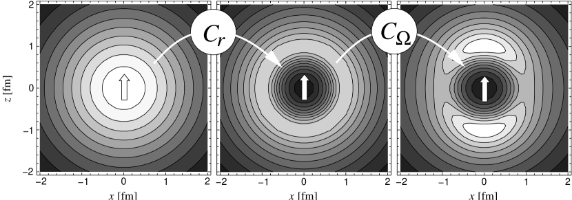
Figure 2: Two-body density $\rho^{(2)}_{S,M_{S},T,M_{T}}(\boldsymbol{{r}})$ in the $S,M_{S}=1,1$; $T,M_{T}=0,0$ channel of $\@@nuc{4}{He}$. Left: uncorrelated trial state $\big{|}\,{\Psi}\,\big{>}$, middle: after radial correlation $C_{r}\big{|}\,{\Psi}\,\big{>}$, and right: with additional tensor correlations $\big{|}\,{\hat{\Psi}}\,\big{>}=C_{\Omega}C_{r}\big{|}\,{\Psi}\,\big{>}$. The arrow indicates the direction of the spin $\boldsymbol{{S}}$. The correlation operator is determined for the Argonne V18 interaction.

The correlated many-body trial state

$$\big{|}\,{\hat{\Psi}}\,\big{>}={C}\big{|}\,{\Psi}\,\big{>}$$ (7)

consists of two parts, the correlator ${C}$ and the uncorrelated trial state $\big{|}\,{\Psi}\,\big{>}$. In the sense of the Ritz variational principle both can be varied. The optimal correlator will however depend on the restrictions imposed on $\big{|}\,{\Psi}\,\big{>}$. Or in other words: The more variational freedom is in $\big{|}\,{\Psi}\,\big{>}$ the less remains for ${C}$. It is important to note that for trial states $\big{|}\,{\Psi}\,\big{>}$ consisting of a superposition of few or many or even very many Slater determinants the corresponding correlators ${C}$ differ only in their long range behavior and are very similar at short distances.

The correlator is the exponential of a two-body operator and therefore the correlated Hamilton operator contains not only one- and two-body but in principle also higher-order contributions. If the correlators are of short-range and the densities are not too high, i.e. the mean distance of the nucleons is larger than the correlation length, the two-body approximation, where only the one- and two-body contributions are taken into account, is well justified. In this two-body approximation the radial and the tensor correlations are evaluated analytically in the angular momentum representation without further approximations in Sec. 4.4.

In Sec. 5 we apply the unitary correlation operator method (UCOM) to the Bonn-A and Argonne V18 interaction which agree in their phase shifts but differ with respect to short-range repulsion and the strength of the tensor interaction. Based on this we perform in Sec. 6 ab initio calculations for the doubly magic nuclei $\@@nuc{4}{He}$, $\@@nuc{16}{O}$ and $\@@nuc{40}{Ca}$ where we use a single Slater determinant of harmonic oscillator shell-model states.

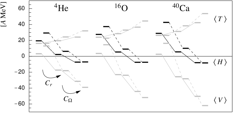
Figure 3: Kinetic $\big{<}\,{{T}}\,\big{>}$, potential $\big{<}\,{{V}}\,\big{>}$ and total energies $\big{<}\,{{H}}\,\big{>}$ obtained with the Bonn-A (left bars in each column connected by full lines) and the Argonne V18 (right bars connected by dashed lines) interaction for the doubly-magic nuclei $\@@nuc{4}{He}$, $\@@nuc{16}{O}$ and $\@@nuc{40}{Ca}$. For each nucleus the energies obtained with uncorrelated, radially correlated and finally with radially and tensorially correlated trial states are displayed.

The effect of the unitary correlator on the kinetic and potential energy is summarized in Fig. 3. In case of the Bonn-A interaction the radial correlator ${C}_{r}^{\phantom{\dagger}}$ that tames the repulsive core reduces the potential energy by about $20-30\;\mathrm{MeV}$ per nucleon in all three nuclei compared to the expectation value of the bare interaction. At the same time the kinetic energy rises only by about $5\;\mathrm{MeV}$ per nucleon. The nuclei are however still unbound after inclusion of the radial correlations (depicted in Fig. 2). The introduction of the tensor correlations, i.e. the alignment of spins along the distance vector between particle pairs, leads to an increase in binding by about $15-25\;\mathrm{MeV}$ per nucleon while the kinetic energy goes up by $5-10\;\mathrm{MeV}$. Now the nuclei are bound at about $-8\;\mathrm{MeV}$ per nucleon. The Argonne V18 induces stronger correlations than the Bonn-A interaction and the radial correlations lower the potential energy by about $30-40\;\mathrm{MeV}$ per nucleon, the tensor correlations give additional $20-30\;\mathrm{MeV}$ per nucleon. At the same time the kinetic energy is increased by $6-12\>\mathrm{MeV}$ (radial correlations) and $8-15\>\mathrm{MeV}$ (tensor correlations). Despite the large differences in potential and kinetic energies the net binding energies obtained by the Bonn-A and the Argonne V18 interaction are almost identical.

We demonstrate in Sec. 5.6 the effects of the correlator in coordinate and momentum space representation and find that the correlated Bonn-A and Argonne V18 interactions agree very well in glaring contrast to the bare interactions. The correlated interactions in momentum space are also compared with the $V_{\mathit{low-k}}$ potential [13] that is obtained by integrating out the high momentum modes. Although derived in a quite different scheme the $V_{\mathit{low-k}}$ potential is very similar to our correlated potential.

The case of $\@@nuc{4}{He}$, where exact results are available, is discussed in detail in Sec. 6, $\@@nuc{16}{O}$ and $\@@nuc{40}{Ca}$ are also calculated. Despite the oversimplified trial state the energy and radii compare very favorably with other much more expensive methods. We also observe that the correlated Argonne V18 and Bonn-A interaction interactions give almost identical results for the nuclei although the corresponding uncorrelated potentials (see Sec. 2) and their expectation values differ greatly. As in the GFMC calculations for light nuclei and the CBF calculations, that are numerically feasible only for $\@@nuc{16}{O}$ and $\@@nuc{40}{Ca}$, when compared to experimental data the nuclei are not bound enough with realistic interactions.

In Sec. 6.3 we calculate the single-particle momentum distribution of the correlated trial states for $\@@nuc{4}{He}$ and $\@@nuc{16}{O}$. We find good agreement with variational Monte-Carlo [14] and spectral function analysis results [15].

We conclude from these observations that the unitary correlator extracts the common low-momentum behaviour of the Bonn-A and the Argonne V18 interactions. With the unitary correlator we therefore have successfully performed a separation of scales. The high-momentum scale of the short-range correlations is covered by the unitary correlator, the low-momentum or long-range behavior is described by the uncorrelated many-body trial state

However the tensor correlations are longer in range than the radial correlations and the separation in short-range or high-momentum components and long-range or low-momentum components as it is possible for the radial correlations is not as clear cut for the tensor correlations. We can ensure the validity of the two-body approximation by using the unitary correlator only for the shorter part of the tensor correlations and use an improved many-body description for the long ranged part of the tensor correlations. Nevertheless a decent description is also possible with very simple many-body trial states and a long ranged tensor correlator when we tolerate larger uncertainties due to three-body contributions to the correlated Hamiltonian.

The fact that realistic two-body forces alone give not enough binding in the many-body system is unfortunate because it implies that additional genuine three-body forces have to be added. In principle Chiral Perturbation Theory should be able to provide a derivation of three-body forces that are consistent with the two-body forces. Because of the complexity of this approach a more phenomenological ansatz for three-body forces is used [16] whose parameters are adjusted to reproduce the many-body properties. The three-body contributions are small compared to the two-body ones. Because of the large cancellations between kinetic and potential energy the three-body forces are nevertheless important for an accurate description of nuclei.

1.3 Summary

The unitary correlator provides a transparent and powerful method to use realistic nucleon-nucleon interactions in ab initio calculations for larger nuclei, but with comparatively little numerical effort. The big advantage of realistic interactions for nuclear structure calculations is that the spin and isospin dependence of the correlated two-body force is fixed. Different from effective interactions or mean-field parameterizations of the energy-density there are no free parameters in the two-body force. This is especially important for the predictions concerning exotic nuclei with large isospins and low density tails.

Our results show in agreement with GFMC calculations of light nuclei that the realistic two-body forces alone cannot successfully reproduce the experimental binding energies of the nuclei.

The ab initio calculations for $\@@nuc{4}{He}$, $\@@nuc{16}{O}$ and $\@@nuc{40}{Ca}$ demonstrate nevertheless that a correlated realistic interaction is a very good starting point. The main problem, the short range repulsion and the short range part of the tensor correlations is successfully tackled by the unitary correlator. What remains to do is the inclusion of three-body forces and improvements in the uncorrelated trial state that take better account of the long range correlations.

2 Nucleon-nucleon interaction

It has been proposed by Weinberg [17, 18] that in the low energy regime of nuclear physics ($\leq 1\;\mathrm{GeV}$) where the appropriate degrees of freedom are the nucleons and the pions one can describe those by an effective field theory based on broken chiral symmetry. In such a scheme the general structure of the nucleon-nucleon interaction is obtained by including all terms up to a certain order that are compatible with the symmetries of the $\pi$-$N$-Lagrangian. The parameters in this effective field theory are determined from the low-energy observables like scattering data. Work is under way to derive the short range part of the nucleon-nucleon potential following these ideas [1]. Another encouraging aspect of this approach is that it allows to determine the structure of the three-body forces on the same footing – at least in principle. Up today this promising method cannot yet compete with the “established” nucleon-nucleon interactions in reproducing the well known scattering data.

Two prominent interactions of the 80’s, that fit the nucleon-nucleon scattering data up to $300\;\mathrm{MeV}$ and the deuteron properties, are the Bonn-A [2] and the Argonne V14 [4] interactions. With more precise and better analyzed scattering data improved versions of these interactions which include additional charge independence breaking and charge symmetry breaking components have been presented in the 90’s, namely the Bonn-CD [3] and the Argonne V18 [5] potential.

In the Bonn approach the nuclear interaction is described in the meson-exchange picture. This includes also higher orders like the correlated two pion-exchange. In the end the interaction is parameterized by one-boson exchange in a relativistic treatment. The nonrelativistic variant of the Bonn interaction has nonlocal momentum dependent terms which appear as relativistic corrections. The nonrelativistic Argonne interaction on the other hand is rather phenomenological. The long range part of the interaction is given as in the Bonn potential by pion exchange, the short-range part is modeled differently, where the Bonn interaction generates repulsion by momentum-dependent interaction terms the Argonne interaction has repulsive local contributions. Nevertheless both describe the measured phase shifts equally well. The potentials are therefore identical on-shell but they differ in their off-shell behavior which matters for nucleons interacting inside bound nuclei. For example, three-body forces that are added to reproduce the experimental binding energies and radii of light nuclei [19, 20, 16] depend on the choice of the two-body force.

Thus the nuclear force is not uniquely determined by the scattering data. We want to remark that the Unitary Correlation Operator Method presented in this work allows the construction of a manifold of two-body interactions ${\hat{H}}={{{C}}}^{{\dagger}}{H}{C}$ which are all phase shift equivalent because our correlator is of finite range, i.e. ${C}(r\rightarrow\infty)={1}$.

2.1 Bonn potentials

Figure 4: Central potential in the $S=0$ and the $S=1$ channels for the Bonn-A interaction (8) (left hand side) and the Argonne V18 interaction (9) (right hand side).

Figure 5: Tensor potential for the Bonn-A interaction (8) (left hand side) and the Argonne V18 interaction (9) (right hand side).

Figure 6: Spin-orbit potential for the Bonn-A interaction (8) (left hand side) and the Argonne V18 interaction (9) (right hand side). The spin-orbit part contained in the $(\boldsymbol{{l}}\!\cdot\!\boldsymbol{{s}})^{2}$ potential has been added for the Argonne V18 potential.

Figure 7: Momentum-dependent potential ($p^{2}$) of the Bonn-A interaction (8) (left hand side). For better comparison with the $l^{2}$ potential of the Argonne V18 interaction (9) the radial dependence of the potential is divided by $r^{2}$. In the $S=1$ channels the $\boldsymbol{{l}}^{2}$ part of the $(\boldsymbol{{l}}\!\cdot\!\boldsymbol{{s}})^{2}$ potential has been added for the Argonne V18. Only the Argonne V18 potential has an $s_{\!12}(\boldsymbol{{l}},\boldsymbol{{l}})$ potential (right) from the decomposition of the $(\boldsymbol{{l}}\!\cdot\!\boldsymbol{{s}})^{2}$ operator.

Out of the family of the Bonn potentials we will use the (nonrelativistic) Bonn-A interaction [2] which has strong nonlocal contributions and a relatively weak tensor force. Because of the technical problems arising from the nonlocal terms there are only a few many-body calculations using the Bonn-A potential in the literature.

We use the more convenient representation of the interaction that projects the potential on spin- and isospin-channels instead of the $\boldsymbol{{\sigma}}\!\cdot\!\boldsymbol{{\sigma}}$ and $\boldsymbol{{\tau}}\!\cdot\!\boldsymbol{{\tau}}$ or the exchange operators

$${v}= \sum_{S,T}v^{c}_{ST}(r)\,\Pi_{ST}+\sum_{T}v^{t}_{1T}(r)\,s_{\!12}(\hat{\boldsymbol{{r}}},\hat{\boldsymbol{{r}}})\,\Pi_{1T}+\sum_{T}v^{b}_{1T}(r)\,\boldsymbol{{l}}\!\cdot\!\boldsymbol{{s}}\,\Pi_{1T}$$ (8)

$$+\sum_{S,T}\frac{1}{2}\left(\boldsymbol{{p}}^{2}v^{p^{2}}_{ST}(r)+v^{p^{2}}_{ST}(r)\boldsymbol{{p}}^{2}\right)\Pi_{ST}\;.$$

The operators $\Pi_{ST}$ project on the respective $S,T$ channels. The nonlocal $\boldsymbol{{p}}^{2}$ dependent terms of the Bonn potential are actually independent of the spin.

The radial dependences in this parameterization are shown in Figs. 4–7 together with the plots for the Argonne V18 interaction.

The Bonn-CD interaction [3], that has been refitted to the new set of scattering data and includes additional charge independence breaking and charge symmetry breaking parts, is unfortunately not given in a nonrelativistic parameterization. Therefore we shall use only the Bonn-A potential in our nonrelativistic approach.

2.2 Argonne potentials

Unlike the Bonn interaction the Argonne V14 interaction [4] is designed to be as local as possible which has technical advantages in GFMC calculations. However momentum dependence is needed to reproduce the phase-shifts. In the Argonne potentials this is included via angular momentum dependence in form of $\boldsymbol{{l}}^{2}$ and $(\boldsymbol{{l}}\!\cdot\!\boldsymbol{{s}})^{2}$ terms in contrast to the $\boldsymbol{{p}}^{2}$ terms of the Bonn interaction.

The Argonne V14 potential can be written in the spin- and isospin channel representation as

$${v}= \sum_{S,T}v^{c}_{ST}(r)\,\Pi_{ST}+\sum_{T}v^{t}_{1T}(r)\,s_{\!12}(\hat{\boldsymbol{{r}}},\hat{\boldsymbol{{r}}})\,\Pi_{1T}+\sum_{T}v^{b}_{1T}(r)\,\boldsymbol{{l}}\!\cdot\!\boldsymbol{{s}}\,\Pi_{1T}$$ (9)

$$+\sum_{S,T}v^{l^{2}}_{ST}(r)\,\boldsymbol{{l}}^{2}\,\Pi_{ST}+\sum_{T}v^{bb}_{1T}(r)\,(\boldsymbol{{l}}\!\cdot\!\boldsymbol{{s}})^{2}\,\Pi_{1T}\;.$$

We decompose the $(\boldsymbol{{l}}\!\cdot\!\boldsymbol{{s}})^{2}$ operator into irreducible tensor operators

$$(\boldsymbol{{l}}\!\cdot\!\boldsymbol{{s}})^{2}=\frac{2}{3}\boldsymbol{{l}}^{2}\,\Pi_{S=1}-\frac{1}{2}\boldsymbol{{l}}\!\cdot\!\boldsymbol{{s}}+\frac{1}{6}s_{\!12}(\boldsymbol{{l}},\boldsymbol{{l}})$$ (10)

and for a proper comparison add the $\boldsymbol{{l}}^{2}$ and $\boldsymbol{{l}}\!\cdot\!\boldsymbol{{s}}$ terms to the respective potential terms in Fig. 6 and 7.

The improved Argonne V18 interaction [5] fitted to the improved scattering data includes the electro-magnetic interaction beyond the static approximation and contains terms that break charge independence and charge symmetry. These additional terms give only minor corrections and we will use the Argonne V18 interactions without those.

A simplified version of the Argonne V18 is the Argonne V8’ interaction [19]. In the Argonne V8’ the $\boldsymbol{{l}}^{2}$ and $(\boldsymbol{{l}}\!\cdot\!\boldsymbol{{s}})^{2}$ parts of the full Argonne V18 interaction are projected onto the central, tensor and spin-orbit parts in such a way that the interaction is unchanged in the $s$- and $p$- waves and in the deuteron channel.

$$v^{c}_{00}(r) \longleftarrow v^{c}_{00}(r)+2v^{l^{2}}_{00}(r)\qquad v^{c}_{01}(r) \longleftarrow v^{c}_{01}(r)$$

$$v^{c}_{10}(r) \longleftarrow v^{c}_{10}(r)\qquad v^{c}_{11}(r) \longleftarrow v^{c}_{11}(r)+2v^{l^{2}}_{11}(r)+\frac{4}{3}v^{bb}_{11}(r)$$

$$v^{t}_{10}(r) \longleftarrow v^{t}_{10}(r)\qquad v^{t}_{11}(r) \longleftarrow v^{t}_{11}(r)-\frac{5}{12}v^{bb}_{11}(r)$$

$$v^{b}_{10}(r) \longleftarrow v^{b}_{10}(r)-2v^{l^{2}}_{10}(r)-3v^{bb}_{10}(r)\qquad v^{b}_{11}(r) \longleftarrow v^{b}_{11}(r)-\frac{1}{2}v^{bb}_{11}(r)$$ (11)

3 Unitary correlation operator method

With the Unitary Correlation Operator Method (UCOM) we want to bring together realistic nuclear interactions and the simple many-body states of a mean-field or shell-model calculation. The short-range or high-momentum properties of the many-body state are treated by the unitary correlator which is almost independent on the low energy scale of the long-range correlations that can be successfully described in a mean-field approach.

The correlated many-body states are constructed by applying the unitary correlation operator ${C}$ to the uncorrelated many-body state $\big{|}\,{\Psi}\,\big{>}$ that may for example be a Slater determinant of harmonic oscillator states as used in shell model calculations or a Slater determinant of Gaussian wave packets as used in the Fermionic Molecular Dynamics (FMD) model

$$\big{|}\,{\hat{\Psi}}\,\big{>}={C}\big{|}\,{\Psi}\,\big{>}\;.$$ (12)

Alternatively we can apply the correlations to the operators and define correlated operators

$${\hat{A}}={{{C}}}^{{\dagger}}{A}{C}\;.$$ (13)

Due to the unitarity of the correlation operator we can evaluate matrix elements either using uncorrelated operators and correlated states or using correlated operators and uncorrelated states:

$$\big{<}\,{\Phi}\,\big{|}\,{{{{C}}}^{{\dagger}}{A}{C}}\,\big{|}\,{\Psi}\,\big{>}=\big{<}\,{\hat{\Phi}}\,\big{|}\,{{A}}\,\big{|}\,{\hat{\Psi}}\,\big{>}=\big{<}\,{\Phi}\,\big{|}\,{{\hat{A}}}\,\big{|}\,{\Psi}\,\big{>}\;.$$ (14)

As the correlation operator ${C}$ should be unitary and describe two-body correlations we will use hermitian two-body generators ${G}_{\Omega}$ and ${G}_{r}$

$${C}={C}_{\Omega}^{\phantom{\dagger}}{C}_{r}^{\phantom{\dagger}}\qquad\textrm{with}\quad{C}_{\Omega}^{\phantom{\dagger}}=\exp\bigl{\{}-\mathrm{i}{G}_{\Omega}\bigr{\}}\qquad\textrm{and}\quad{C}_{r}^{\phantom{\dagger}}=\exp\bigl{\{}-\mathrm{i}{G}_{r}\bigr{\}}\;.$$ (15)

The correlation operator ${C}$ itself is not a two-body operator because the repetitive application of the generator produces operators of increasing order in particle number. If we want to describe genuine three-body correlations we would have to use three-body operators in the generators ${G}$.

The correlated Hamilton operator should posses the same symmetries with respect to global transformations like translation, rotation, or boost as the uncorrelated one. Therefore the generator can only depend on the relative coordinates and momenta of the two particles and it has to be a scalar operator with respect to rotations. Furthermore the correlations should fulfill the cluster decomposition property, which implies that observables in subsystems, that are mutually outside the range of the interaction, are not affected by the other subsystems. The correlations therefore have to be of finite range.

Before we look at the explicit form of the generators for radial and tensor correlators we discuss the application of correlated operators in many-body systems, which is performed in the sense of the cluster expansion.

3.1 Cluster expansion

As the correlation operator ${C}$ is the exponential of a two-body operator, the correlation operator itself and correlated operators have irreducible contributions of higher particle orders. The Fock space representation of the correlated operator ${\hat{A}}$ is given by the cluster expansion

$${\hat{A}}={{{C}}}^{{\dagger}}{A}{C}=\sum_{i=1}{\hat{A}}^{[i]}\;,$$ (16)

where $i$ denotes the irreducible particle number.

Using an orthonormal one-body basis $\bigl{\{}\big{|}\,{k}\,\big{>}={a}^{\dagger}_{k}\big{|}\,{0}\,\big{>}\bigr{\}}$ we get

$${\hat{A}}^{[1]} =\sum_{k,k^{\prime}}\big{<}\,{k}\,\big{|}\,{{{{C}}}^{{\dagger}}{A}{C}}\,\big{|}\,{k^{\prime}}\,\big{>}\;{a}^{\dagger}_{k}{a}^{\phantom{\dagger}}_{k^{\prime}}=\sum_{k,k^{\prime}}\big{<}\,{k}\,\big{|}\,{{A}}\,\big{|}\,{k^{\prime}}\,\big{>}\;{a}^{\dagger}_{k}{a}^{\phantom{\dagger}}_{k^{\prime}}$$ (17)

$${\hat{A}}^{[2]} =\frac{1}{4}\sum_{\begin{subarray}{c}k_{1},k_{2}\\ k_{1}^{\prime},k_{2}^{\prime}\end{subarray}}{}_{a}\big{<}\,{k_{1},k_{2}}\,\big{|}\,{{{{C}}}^{{\dagger}}{A}{C}-{\hat{A}}^{[1]}}\,\big{|}\,{k_{1}^{\prime},k_{2}^{\prime}}\,\big{>}{}_{a}\;{a}^{\dagger}_{k_{1}}{a}^{\dagger}_{k_{2}}{a}^{\phantom{\dagger}}_{k_{2}^{\prime}}{a}^{\phantom{\dagger}}_{k_{1}^{\prime}}$$ (18)

$$\vdots$$

$${\hat{A}}^{[n]} =\frac{1}{(n!)^{2}}\sum_{\begin{subarray}{c}k_{1},\ldots,k_{n}\\ k_{1}^{\prime},\ldots,k_{n}^{\prime}\end{subarray}}{}_{a}\big{<}\,{k_{1},\ldots,k_{n}}\,\big{|}\,{{{{C}}}^{{\dagger}}{A}{C}-\sum_{i=1}^{n-1}{\hat{A}}^{[i]}}\,\big{|}\,{k_{1}^{\prime},\ldots,k_{n}^{\prime}}\,\big{>}{}_{a}\;{a}^{\dagger}_{k_{1}}\cdots{a}^{\dagger}_{k_{n}}\,{a}^{\phantom{\dagger}}_{k_{n}^{\prime}}\cdots{a}^{\phantom{\dagger}}_{k_{1}^{\prime}}\;,$$ (19)

where at each order of the cluster expansion the contributions of the lower particle orders have to be subtracted.

In practice we would like to restrict the calculations to the two-body level as the three-body contributions are already very involved. We should therefore use generators ${G}$ which cause only small three-body contributions. The importance of three-body contributions will increase with the range of the correlator and the density of the system.

We will use the notation

$$\left[{{{C}}}^{{\dagger}}{A}{C}\right]^{C2}={\hat{A}}^{[1]}+{\hat{A}}^{[2]}$$ (20)

to indicate the two-body approximation.

3.2 Two-body system

For calculating many-body matrix elements in two-body approximation one has to evaluate matrix elements of correlated operators in one- and two-body space only. As defined in Eqs. (17) and (18) those matrix elements then define the one- and two-body operators in Fock space, respectively.

In contrast to Fock space operators which are denoted by uppercase letters (e.g. ${C}$) we will use lowercase letters for operators in one- or two-body space (e.g. ${c}$ for the correlation operator in two-body space).

The correlator affects only the relative and not the center of mass motion of two nucleons. Therefore relative and center of mass variables of two nucleons are introduced:

$$\boldsymbol{{r}} =\boldsymbol{{x}}_{1}-\boldsymbol{{x}}_{2}\;, \qquad\boldsymbol{{x}}_{\mathrm{cm}} =\frac{1}{2}(\boldsymbol{{x}}_{1}+\boldsymbol{{x}}_{2})\;,$$ (21)

$${\boldsymbol{{p}}} =\frac{1}{2}({\boldsymbol{{p}}}_{1}-{\boldsymbol{{p}}}_{2})\;, \qquad{\boldsymbol{{p}}}_{\mathrm{cm}} ={\boldsymbol{{p}}}_{1}+{\boldsymbol{{p}}}_{2}\;.$$ (22)

For example in the kinetic energy

$${t}={t}_{\mathrm{rel}}+{t}_{\mathrm{cm}}\qquad\mathrm{with}\qquad{t}_{\mathrm{rel}}=\frac{1}{m}{\boldsymbol{{p}}}^{2}\;,\qquad{t}_{\mathrm{cm}}=\frac{1}{4m}{\boldsymbol{{p}}}_{\mathrm{cm}}^{2}$$ (23)

only the kinetic energy ${t}_{\mathrm{rel}}$ of the relative motion has to be correlated. The orbital angular momentum of the two-body system can also be decomposed into the orbital angular momentum of the relative motion and the center of mass one

$${\boldsymbol{{l}}}_{1}+{\boldsymbol{{l}}}_{2}={\boldsymbol{{l}}}_{\mathrm{cm}}+{\boldsymbol{{l}}}\qquad\mathrm{with}\qquad{\boldsymbol{{l}}}={\boldsymbol{{r}}}\times{\boldsymbol{{p}}}\;,\qquad{\boldsymbol{{l}}}_{\mathrm{cm}}={\boldsymbol{{x}}}_{\mathrm{cm}}\times{\boldsymbol{{p}}}_{\mathrm{cm}}\;.$$ (24)

As we want to study correlations induced by the nuclear force, which in two-body space does not connect states of different total spin and isospin, we use in the following the basis states $\big{|}\,{n;(LS)JM;TM_{T}}\,\big{>}$ with quantum numbers $L,M_{L}$ for relative angular momentum, $S,M_{S}$ for total spin, $J,M$ for total angular momentum, and $T,M_{T}$ for total isospin. With the help of Clebsch-Gordan coefficients their coordinate representation is given by

$$\big{<}\,{\boldsymbol{{x}}_{1},\boldsymbol{{x}}_{2}}\,\big{|}\,{n;(LS)JM;TM_{T}}\,\big{>}=\\ \varphi^{n}_{(LS)J,T}(r)\!\sum_{M_{L},M_{S}}\mathrm{C}\Biggl{(}\,\begin{matrix}{L}&{S}\\ {M_{L}}&{M_{S}}\end{matrix}\,\Biggr{|}\Biggl{.}\,\begin{matrix}{J}\\ {M}\end{matrix}\,\Biggr{)}Y_{LM_{L}}(\hat{\boldsymbol{{r}}})\big{|}\,{SM_{S}}\,\big{>}\big{|}\,{TM_{T}}\,\big{>}\,\phi_{\mathrm{cm}}(\boldsymbol{{x}}_{\mathrm{cm}})\;,$$ (25)

where $Y_{LM_{L}}(\hat{\boldsymbol{{r}}})$ denotes spherical harmonics that depend on the unit vector of the relative coordinate. The quantum numbers of the center of mass motion are indicated only when needed.

The transformation back to one-body variables with spin components $\chi_{i}$ and isospin components $\xi_{i}$ is obtained from

$$\big{<}\,{\boldsymbol{{x}}_{1}\chi_{1}\xi_{1};\boldsymbol{{x}}_{2}\chi_{2}\xi_{2}}\,\big{|}\,{\phi}\,\big{>}=\\ \sum_{S,M_{S}}\mathrm{C}\Biggl{(}\,\begin{matrix}{{\textstyle\frac{1}{2}}}&{{\textstyle\frac{1}{2}}}\\ {\chi_{1}}&{\chi_{2}}\end{matrix}\,\Biggr{|}\Biggl{.}\,\begin{matrix}{S}\\ {M_{S}}\end{matrix}\,\Biggr{)}\sum_{T,M_{T}}\mathrm{C}\Biggl{(}\,\begin{matrix}{{\textstyle\frac{1}{2}}}&{{\textstyle\frac{1}{2}}}\\ {\xi_{1}}&{\xi_{2}}\end{matrix}\,\Biggr{|}\Biggl{.}\,\begin{matrix}{T}\\ {M_{T}}\end{matrix}\,\Biggr{)}\big{<}\,{\boldsymbol{{r}}\,\boldsymbol{{x}}_{\mathrm{cm}};SM_{S};TM_{T}}\,\big{|}\,{\phi}\,\big{>}\;.$$ (26)

3.3 Spin-isospin dependent correlators

As the nuclear force depends strongly on spin and isospin the correlations will be distinct in the different spin-isospin channels. In two-body space we use the ansatz

$${g}=\sum_{ST}{g}_{ST}\,{\Pi}_{ST}$$ (27)

for a spin-isospin dependent generator with the projectors ${\Pi}_{ST}$ on the spin-isospin channels. Exploiting the projector properties we can rewrite the correlation operator

$${c}=\exp\big{\{}-\mathrm{i}{g}\bigr{\}}=\sum_{ST}\exp\bigl{\{}-\mathrm{i}{g}_{ST}\bigr{\}}\,{\Pi}_{ST}\;,$$ (28)

and as the nuclear interaction does not connect the different spin and isospin channels we obtain the correlated potential in two-body space as

$${\hat{v}}={{{c}}}^{{\dagger}}{v}{c}=\sum_{ST}\exp\bigl{\{}\mathrm{i}{g}_{ST}\bigr{\}}\>{v}_{ST}\>\exp\bigl{\{}-\mathrm{i}{g}_{ST}\bigr{\}}\,{\Pi}_{ST}\;.$$ (29)

We have thus the important result that the correlations in the different spin-isospin channels decouple and the correlation operators can be determined for each spin-isospin channel independently.

3.4 Correlated densities

The short-range radial and tensor correlations in the nucleus can be studied best by inspecting the one- and two-body density matrices. The density matrices of the many-body state $\big{|}\,{\Phi}\,\big{>}$ in coordinate representation are defined as

$$\rho^{(1)}(\boldsymbol{{x}}_{1}\chi_{1}\xi_{1};\boldsymbol{{x}}_{1}^{\prime}\chi_{1}^{\prime}\xi_{1}^{\prime})=\big{<}\,{\Phi}\,\big{|}\,{{\Psi}^{\dagger}_{\chi_{1}^{\prime}\xi_{1}^{\prime}}(\boldsymbol{{x}}_{1}^{\prime}){\Psi}^{\phantom{\dagger}}_{\chi_{1}\xi_{1}}(\boldsymbol{{x}}_{1})}\,\big{|}\,{\Phi}\,\big{>}$$ (30)

and

$$\rho^{(2)}(\boldsymbol{{x}}_{1}\chi_{1}\xi_{1},\boldsymbol{{x}}_{2}\chi_{2}\xi_{2};\boldsymbol{{x}}_{1}^{\prime}\chi_{1}^{\prime}\xi_{1}^{\prime},\boldsymbol{{x}}_{2}^{\prime}\chi_{2}^{\prime}\xi_{2}^{\prime})=\\ \big{<}\,{\Phi}\,\big{|}\,{{\Psi}^{\dagger}_{\chi_{1}^{\prime}\xi_{1}^{\prime}}(\boldsymbol{{x}}_{1}^{\prime}){\Psi}^{\dagger}_{\chi_{2}^{\prime}\xi_{2}^{\prime}}(\boldsymbol{{x}}_{2}^{\prime}){\Psi}^{\phantom{\dagger}}_{\chi_{2}\xi_{2}}(\boldsymbol{{x}}_{2}){\Psi}^{\phantom{\dagger}}_{\chi_{1}\xi_{1}}(\boldsymbol{{x}}_{1})}\,\big{|}\,{\Phi}\,\big{>}\;,$$ (31)

where ${\Psi}^{\phantom{\dagger}}_{\chi\xi}(\boldsymbol{{x}})$ is the field operator for a nucleon with spin component $\chi$ and isospin component $\xi$ at position $\boldsymbol{{x}}$.

The two-body correlations can be visualized best with the help of the two-body density matrix $\rho^{(2)}_{SM_{S},TM_{T}}(\boldsymbol{{r}})$ which describes the probability density to find two nucleons at a distance $\boldsymbol{{r}}$ in the $S,T$ channel with spin and isospin orientations $M_{S},M_{T}$. The center of mass coordinate is integrated out.

$$\rho^{(2)}_{SM_{S},TM_{T}}(\boldsymbol{{r}})=\sum_{\chi_{1},\chi_{2}}\mathrm{C}\Biggl{(}\,\begin{matrix}{{\textstyle\frac{1}{2}}}&{{\textstyle\frac{1}{2}}}\\ {\chi_{1}}&{\chi_{2}}\end{matrix}\,\Biggr{|}\Biggl{.}\,\begin{matrix}{S}\\ {M_{S}}\end{matrix}\,\Biggr{)}\sum_{\xi_{1},\xi_{2}}\mathrm{C}\Biggl{(}\,\begin{matrix}{{\textstyle\frac{1}{2}}}&{{\textstyle\frac{1}{2}}}\\ {\xi_{1}}&{\xi_{2}}\end{matrix}\,\Biggr{|}\Biggl{.}\,\begin{matrix}{T}\\ {M_{T}}\end{matrix}\,\Biggr{)}\\ \times\int\!\mathrm{d}^{3}{X}\;\rho^{(2)}(\boldsymbol{{X}}\!+\!{\textstyle\frac{1}{2}}\boldsymbol{{r}}\chi_{1}\xi_{1},\boldsymbol{{X}}\!-\!{\textstyle\frac{1}{2}}\boldsymbol{{r}}\chi_{2}\xi_{2};\boldsymbol{{X}}\!+\!{\textstyle\frac{1}{2}}\boldsymbol{{r}}\chi_{1}\xi_{1},\boldsymbol{{X}}\!-\!{\textstyle\frac{1}{2}}\boldsymbol{{r}}\chi_{2}\xi_{2})$$ (32)

The information about the short-range radial correlations is contained in the radial dependence of this two-nucleon correlation function. The tensor correlations manifest themselves by the angular and the spin dependence.

As with other operators the density matrices of correlated many-body states $\big{|}\,{\hat{\Phi}}\,\big{>}={C}\big{|}\,{\Phi}\,\big{>}$ are calculated in the cluster expansion

$$\begin{split}\hat{\rho}^{(1)}(\boldsymbol{{x}}_{1}\chi_{1}\xi_{1};\boldsymbol{{x}}_{1}^{\prime}\chi_{1}^{\prime}\xi_{1}^{\prime})&=\big{<}\,{\Phi}\,\big{|}\,{{{{C}}}^{{\dagger}}{\Psi}^{\dagger}_{\chi_{1}^{\prime}\xi_{1}^{\prime}}(\boldsymbol{{x}}_{1}^{\prime}){\Psi}^{\phantom{\dagger}}_{\chi_{1}\xi_{1}}(\boldsymbol{{x}}_{1}){C}}\,\big{|}\,{\Phi}\,\big{>}\\ &=\sum_{n=1}^{A}\big{<}\,{\Phi}\,\big{|}\,{\bigl{[}{{{C}}}^{{\dagger}}{\Psi}^{\dagger}_{\chi_{1}^{\prime}\xi_{1}^{\prime}}(\boldsymbol{{x}}_{1}^{\prime}){\Psi}^{\phantom{\dagger}}_{\chi_{1}\xi_{1}}(\boldsymbol{{x}}_{1}){C}\bigr{]}^{[n]}}\,\big{|}\,{\Phi}\,\big{>}\;,\end{split}$$ (33)

$$\hat{\rho}^{(2)}(\boldsymbol{{x}}_{1}\chi_{1}\xi_{1},\boldsymbol{{x}}_{2}\chi_{2}\xi_{2};\boldsymbol{{x}}_{1}^{\prime}\chi_{1}^{\prime}\xi_{1}^{\prime},\boldsymbol{{x}}_{2}^{\prime}\chi_{2}^{\prime}\xi_{2}^{\prime})=\\ \begin{split}&=\big{<}\,{\Phi}\,\big{|}\,{{{{C}}}^{{\dagger}}{\Psi}^{\dagger}_{\chi_{1}^{\prime}\xi_{1}^{\prime}}(\boldsymbol{{x}}_{1}^{\prime}){\Psi}^{\dagger}_{\chi_{2}^{\prime}\xi_{2}^{\prime}}(\boldsymbol{{x}}_{2}^{\prime}){\Psi}^{\phantom{\dagger}}_{\chi_{2}\xi_{2}}(\boldsymbol{{x}}_{2}){\Psi}^{\phantom{\dagger}}_{\chi_{1}\xi_{1}}(\boldsymbol{{x}}_{1}){C}}\,\big{|}\,{\Phi}\,\big{>}\\ &=\sum_{n=2}^{A}\big{<}\,{\Phi}\,\big{|}\,{\bigl{[}{{{C}}}^{{\dagger}}{\Psi}^{\dagger}_{\chi_{1}^{\prime}\xi_{1}^{\prime}}(\boldsymbol{{x}}_{1}^{\prime}){\Psi}^{\dagger}_{\chi_{2}^{\prime}\xi_{2}^{\prime}}(\boldsymbol{{x}}_{2}^{\prime}){\Psi}^{\phantom{\dagger}}_{\chi_{2}\xi_{2}}(\boldsymbol{{x}}_{2}){\Psi}^{\phantom{\dagger}}_{\chi_{1}\xi_{1}}(\boldsymbol{{x}}_{1}){C}\bigr{]}^{[n]}}\,\big{|}\,{\Phi}\,\big{>}\;.\end{split}$$ (34)

In the two-body approximation the expansions will be truncated after the second order. One should notice that density matrices calculated in a truncated cluster expansion fulfill the reduction property of the exact density matrices

$$\sum_{\chi_{2},\xi_{2}}\int\!\mathrm{d}^{3}{x_{2}}\;\hat{\rho}^{(2)}(\boldsymbol{{x}}_{1}\chi_{1}\xi_{1},\boldsymbol{{x}}_{2}\chi_{2}\xi_{2};\boldsymbol{{x}}_{1}^{\prime}\chi_{1}^{\prime}\xi_{1}^{\prime},\boldsymbol{{x}}_{2}\chi_{2}\xi_{2})=(A-1)\,\hat{\rho}^{(1)}(\boldsymbol{{x}}_{1}\chi_{1}\xi_{1};\boldsymbol{{x}}_{1}^{\prime}\chi_{1}^{\prime}\xi_{1}^{\prime})$$ (35)

only approximately. If the truncation at second order is justified, Eq. (35) is well approximated.

The nucleon density distribution $\hat{\rho}(\boldsymbol{{x}})$ is given by the diagonal part of the one-body density matrix which has been summed over spin and isospin indices

$$\hat{\rho}(\boldsymbol{{x}})=\sum_{\chi,\xi}\hat{\rho}^{(1)}(\boldsymbol{{x}}\chi\xi;\boldsymbol{{x}}\chi\xi)\ .$$ (36)

The nucleon momentum distribution $\hat{n}(\boldsymbol{{k}})$, displayed for $\@@nuc{4}{He}$ and $\@@nuc{16}{O}$ in Sec. 6.3 is evaluated in momentum-space in two-body approximation

$$\hat{n}(\boldsymbol{{k}})=\sum_{\chi,\xi}\Bigl{(}\big{<}\,{\Phi}\,\big{|}\,{{a}^{\dagger}_{\chi\xi}(\boldsymbol{{k}}){a}^{\phantom{\dagger}}_{\chi\xi}(\boldsymbol{{k}})}\,\big{|}\,{\Pi}\,\big{>}+\\ \int\!\mathrm{d}^{3}{k^{\prime}}\;\sum{\chi^{\prime},\xi^{\prime}}\big{<}\,{\Phi}\,\big{|}\,{\bigl{[}{{{C}}}^{{\dagger}}{a}^{\dagger}_{\chi\xi}(\boldsymbol{{k}}){a}^{\dagger}_{\chi^{\prime}\xi^{\prime}}(\boldsymbol{{k}}^{\prime}){a}^{\phantom{\dagger}}_{\chi^{\prime}\xi^{\prime}}(\boldsymbol{{k}}^{\prime}){a}^{\phantom{\dagger}}_{\chi\xi}(\boldsymbol{{k}}){C}\bigr{]}^{[2]}}\,\big{|}\,{\Phi}\,\big{>}\Bigr{)}$$ (37)

and can be related to the Fourier transform of the off-diagonal matrix elements of the one-body density matrix

$$\hat{n}(\boldsymbol{{k}})=\int\!\mathrm{d}^{3}{x_{1}}\;\int\!\mathrm{d}^{3}{x_{2}}\;\sum_{\chi\xi}\hat{\rho}^{(1)}(\boldsymbol{{x}}_{1}\chi\xi;\boldsymbol{{x}}_{2}\chi\xi)\>e^{i\boldsymbol{{k}}\cdot(\boldsymbol{{x}}_{1}-\boldsymbol{{x}}_{2})}\;.$$ (38)

4 Correlations

All realistic nucleon-nucleon interactions, like the Bonn and the Argonne potentials discussed in Sec. 2, possess a short ranged repulsive core and a tensor force. The repulsion causes an attenuation of the two-body density at short distances while the tensor interaction induces a strong correlation between the spatial orientation of the nucleons and the orientation of their spins. It operates only in the $S=1$ channels but is crucial for a successful description of the nucleus, without the tensor part of the potential nuclei are not bound.

We introduce unitary transformations to create the short range correlations induced by the interaction that are missing in the uncorrelated many-body trial state. This is done by moving the particles subject to their relative distance and their spin directions. It turns out that a separation into shifts parallel and perpendicular to the relative distance leads to a concise operator structure.

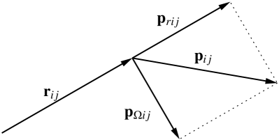
Figure 8: Decomposition of relative momentum ${\boldsymbol{{p}}}_{ij}$ parallel and perpendicular to relative distance ${\boldsymbol{{r}}}_{ij}$.

In order to achieve shifts in the direction of ${\boldsymbol{{r}}}_{ij}={\boldsymbol{{r}}}_{i}-{\boldsymbol{{r}}}_{j}$ and perpendicular to it we decompose the relative momentum operator ${\boldsymbol{{p}}}_{ij}=\frac{1}{2}({\boldsymbol{{p}}}_{i}-{\boldsymbol{{p}}}_{j})$ into a component ${\boldsymbol{{p}}}_{rij}$ that is parallel and a component ${\boldsymbol{{p}}}_{\Omega ij}$ that is orthogonal

$${\boldsymbol{{p}}}_{ij}={\boldsymbol{{p}}}_{rij}+{\boldsymbol{{p}}}_{\Omega ij}$$ (39)

as indicated in Fig. 8. The relative momentum of the pair $(ij)$ in the radial direction is defined by the projection

$${\boldsymbol{{p}}}_{rij}=\frac{\boldsymbol{{r}}_{ij}}{r_{\!ij}}\ {\boldsymbol{{p}}}_{rij}\;,$$ (40)

where the hermitean operator ${p}_{ij}$ for the radial relative momentum is given by

$${p}_{rij}=\frac{1}{2}\biggl{(}\frac{\boldsymbol{{r}}_{ij}}{r_{ij}}{\boldsymbol{{p}}}_{ij}+{\boldsymbol{{p}}}_{ij}\frac{\boldsymbol{{r}}_{ij}}{r_{\!ij}}\biggr{)}\overset{\scriptstyle{\boldsymbol{{r}}}}{\Rightarrow}\biggl{(}\frac{1}{r_{\!ij}}\frac{\partial}{\mathrm{i}\partial r_{\!ij}}r_{\!ij}\biggr{)}\;.$$ (41)

As ${\boldsymbol{{p}}}_{ij}$ and ${\boldsymbol{{r}}}_{ij}$ are operators and do not commute we take the hermitean combination of the classical expressions. The remaining part ${\boldsymbol{{p}}}_{\Omega ij}$ that is perpendicular to $\boldsymbol{{r}}_{ij}$ is

$${\boldsymbol{{p}}}_{\Omega ij}=\frac{1}{2r_{\!ij}}\biggl{(}{\boldsymbol{{l}}_{ij}}\times\frac{{\boldsymbol{{r}}}_{ij}}{{r}_{\!ij}}-\frac{\boldsymbol{{r}}_{ij}}{r_{\!ij}}\times\boldsymbol{{l}}_{ij}\biggr{)}\;.$$ (42)

We call ${\boldsymbol{{p}}}_{\Omega ij}$ relative orbital momentum. It should not be confused with the relative orbital angular momentum ${\boldsymbol{{l}}}_{ij}={\boldsymbol{{r}}}_{ij}\times{\boldsymbol{{p}}}_{ij}$. Both, ${\boldsymbol{{p}}}_{rij}$ and ${\boldsymbol{{p}}}_{\Omega ij}$ are hermitian. We have summarized some properties of these operators in Appendix A.1.

The radial relative momentum ${p}_{rij}$ will be used in ${C}_{r}^{\phantom{\dagger}}$ as the generator of radial shifts that move the particle pair $(ij)$ out of their mutual repulsive interaction area, see Eq. (4). The orbital relative momentum ${\boldsymbol{{p}}}_{\Omega ij}$ in combination with the spin operators ${\boldsymbol{{\sigma}}}_{i}$ and ${\boldsymbol{{\sigma}}}_{j}$ will be used in the unitary transformation ${C}_{\Omega}^{\phantom{\dagger}}$ (Eq. (6)) to relocate the angular position of the pair to regions where the tensor interaction is attractive.

The correlator ${C}={C}_{\Omega}^{\phantom{\dagger}}{C}_{r}^{\phantom{\dagger}}$ has to be of finite range for the application in the many-body system in order not to destroy the cluster decomposition property. The task of the unitary correlation operators is to introduce the short-range repulsive and tensor correlations into the many-body state. Possible long range correlations should be described by the many-body trial state and not by the correlation operator. If analyzed in momentum space the correlator describes the high momentum components of the state while the low momentum part is taken care of by the model space.

In the following we restrict the investigations to the two-body space as this is sufficient for a cluster expansion up to two-body contributions. We use lower case letters for the operators to indicate that and omit the indices $(ij)=(12)$ for the particles.

4.1 Radial correlations

Radial correlations within the UCOM framework have already been studied in detail in Refs. [12, 21]. In this section we shall only provide a short summary of the ideas and techniques. For the illustrations we use the Argonne V18 potential in the $S,T=0,1$ channel (for $L=0$ identical to the Argonne V8’ potential) where we do not have to deal with additional correlations from tensor interactions.

The strong repulsion at short distances is suppressing the two-body density in the range of the core as already shown in Fig. 1. To describe these short-range correlations the radial correlator

$${c}_{r}^{\phantom{\dagger}}=\exp\bigl{\{}-\mathrm{i}\,{g}_{r}\bigr{\}}=\exp\Bigl{\{}-\mathrm{i}\frac{1}{2}\bigl{(}{p}_{r}s({r})+s({r}){p}_{r}\bigr{)}\Bigr{\}}$$ (43)

(c.f. Eq. (4)) shifts nuleons that are in the range of the repulsive core radially outwards while those being already further out are not affected. To achieve this the generator ${g}_{r}$ contains the radial momentum operator ${p}_{r}$ and the shift function $s(r)$ which tends to zero for large $r$. (see also Appendix A.1 for further properties)

It is advantageous to introduce the correlation functions $R_{+}(r)$ and $R_{-}(r)$ which are related to the shift function $s(r)$ by

$$\pm 1=\int_{r}^{R_{\pm}(r)}\frac{d\xi}{s(\xi)}\;.$$ (44)

The correlation functions are mutually inverse to each other

$$R_{\pm}(R_{\mp}(r))=r\;,$$ (45)

which reflects the unitarity of the correlation operator. For small shifts one has approximately

$$R_{\pm}(r)\approx r\pm s(r)\;.$$ (46)

Figure 9: Left: correlation function $R_{+}^{01}(r)$ and its inverse $R_{-}^{01}(r)$ for the Argonne V18 potential in the $S,T=0,1$ channel. Right: Correlated (dotted) and uncorrelated (solid) Gaussian and constant wave functions.

The correlation functions $R_{+}(r)$ and $R_{-}(r)$ for the $S,T=0,1$ channel of the Argonne V18 potential are displayed in Fig. 9. The radial shift is strongest in the range up to about $0.5\;\mathrm{fm}$ and extends to about $1.5\;\mathrm{fm}$. On the right hand side of Fig. 9 a correlated Gaussian wave function and a correlated constant wave function are displayed. The correlated wave functions are almost identical in the range of the repulsive core of the interaction. As the correlator conserves the norm of the wave function the hole created at short distances has to be compensated by an enhancement of the wave function further out.

In the case of radial correlations it is possible to give closed expressions for all operators in coordinate representation [12], like

$${c}_{r}^{\dagger}\,r\,{c}_{r}^{\phantom{\dagger}} =R_{+}(r)\;,\qquad\qquad {c}_{r}^{\dagger}\,\frac{\boldsymbol{{r}}}{r}\,{c}_{r}^{\phantom{\dagger}} =\frac{\boldsymbol{{r}}}{r}\;,$$

$${c}_{r}^{\dagger}\,{p}_{r}\,{c}_{r}^{\phantom{\dagger}} =\frac{1}{\sqrt{R_{+}^{\prime}({r})}}\,{p}_{r}\,\frac{1}{\sqrt{R_{+}^{\prime}({r})}}\;,\qquad\qquad {c}_{r}^{\dagger}\,{\boldsymbol{{p}}}_{\Omega}\,{c}_{r}^{\phantom{\dagger}} ={\boldsymbol{{p}}}_{\Omega}\;,$$

$${c}_{r}^{\dagger}\,{\boldsymbol{{l}}}\,{c}_{r}^{\phantom{\dagger}} ={\boldsymbol{{l}}}\;,\qquad\qquad {c}_{r}^{\dagger}\,{\boldsymbol{{\sigma}}}_{1,2}\,{c}_{r}^{\phantom{\dagger}} ={\boldsymbol{{\sigma}}}_{1,2}\;.$$ (47)

Due to the unitary of ${c}_{r}^{\phantom{\dagger}}$ any combination of operators can be transformed by individual transformations.

The calculation of the correlated kinetic energy in two-body approximation results in a one- and a two-body contribution to the correlated Hamilton operator. The one-body contribution is again the kinetic energy because the generator ${g}_{r}$ is a two-body operator and thus the correlator ${c}_{r}^{\phantom{\dagger}}=\exp\{-\mathrm{i}{g}_{r}\}$ contains besides the unit operator only two-body or higher terms.

$${\hat{t}}^{[1]}={{{c}}}^{{\dagger}}{t}^{[1]}{c}={t}^{[1]}$$ (48)

For the calculation of the two-body contribution of the correlated kinetic energy we use the relative and center of mass variables introduced in Sec. 3.2. The center of mass kinetic energy $t_{\mathrm{cm}}$ is not influenced by the correlator and the kinetic energy of the relative motion can be decomposed further in a radial and an angular part

$${t}_{\mathrm{rel}}={t}_{r}+{t}_{\Omega}=\frac{1}{m}p_{r}^{2}+\frac{1}{m}\frac{\boldsymbol{{l}}^{2}}{r^{2}}\;,$$ (49)

where the angular part is correlated simply by replacing ${r}$ with $R_{+}({r})$ because the relative angular momentum ${\boldsymbol{{l}}}$ commutes with ${c}_{r}^{\phantom{\dagger}}$ (see Eqs. (47)). Thus one obtains the two-body contribution to the radially correlated operator as

$${c}_{r}^{\dagger}{t}_{\Omega}{c}_{r}^{\phantom{\dagger}}-{t}_{\Omega}=\frac{1}{m}\left(\frac{\boldsymbol{{l}}^{2}}{R_{+}(r)^{2}}-\frac{\boldsymbol{{l}}^{2}}{r^{2}}\right)=\frac{1}{2\hat{\mu}_{\Omega}(r)}\frac{\boldsymbol{{l}}^{2}}{r^{2}}$$ (50)

with a correlated “angular mass”

$$\frac{1}{2\hat{\mu}_{\Omega}(r)}=\frac{1}{m}\biggl{(}\frac{r^{2}}{R_{+}(r)^{2}}-1\biggr{)}\;.$$ (51)

The radially correlated radial part of the kinetic energy leads with (47) to a momentum dependent potential

$${c}_{r}^{\dagger}{t}_{r}{c}_{r}^{\phantom{\dagger}}-{t}_{r}=\frac{1}{2}\biggl{[}p_{r}^{2}\frac{1}{2\hat{\mu}_{r}(r)}+\frac{1}{2\hat{\mu}_{r}(r)}p_{r}^{2}\biggr{]}+\hat{w}(r)$$ (52)

similar to the kinetic energy but with a correlated “radial mass”

$$\frac{1}{2\hat{\mu}_{r}(r)}=\frac{1}{m}\biggl{(}\frac{1}{R_{+}^{\prime}(r)^{2}}-1\biggr{)}$$ (53)

and an additional local potential

$$\hat{w}(r)=\frac{1}{m}\biggl{(}\frac{7R_{+}^{\prime\prime}(r)^{2}}{4R_{+}^{\prime}(r)^{4}}-\frac{R_{+}^{\prime\prime\prime}(r)}{2R_{+}^{\prime}(r)^{3}}\biggr{)}\;.$$ (54)

The radially correlated kinetic energy has interaction components that we also find in the uncorrelated Bonn-A interaction (8), but there “radial mass” and “angular mass” are the same. The radial dependence of the $\boldsymbol{{l}}^{2}$ term that is expressed in terms of the “angular mass” $\hat{\mu}_{\Omega\,01}(r)$ corresponds to the $v^{l^{2}}_{01}(r)$ dependence of the Argonne V18 interaction (9). One recognizes that the radial correlation of the kinetic energy introduces momentum dependent interactions of the same type as are already present in the original interaction.

In Fig. 10 the contributions to the correlated kinetic energy of the Argonne V18 interaction are shown. Comparison with Fig. 7 shows that $v^{l^{2}}_{01}(r)$ is of the same order as $1/(2\hat{\mu}_{\Omega\,01}(r)r^{2})$ but of opposite sign. Since the correlated and uncorrelated interactions have the same phase shifts this points already at the ambiguities in trading a local repulsion for a momentum dependence.

Figure 10: Correlated kinetic energy: inverse radial and angular mass divided by $r^{2}$ (left) and potential part (right) for the Argonne V18 potential in the $S,T=0,1$ channel.

The correlated central potential plotted in Fig. 11 is expressed easily with help of relation (47) as the uncorrelated potential with a transformed radial dependence

$${\hat{v}}^{c}={c}_{r}^{\dagger}v^{c}({r}){c}_{r}^{\phantom{\dagger}}=v^{c}(R_{+}(r))\;.$$ (55)

Figure 11: Correlated central potential of the Argonne V18 in the $S,T=0,1$ channel. The central correlator weakens the core of the interaction.

Like for the central interaction, the radially correlated spin-orbit and tensor potentials only have a transformed radial dependence (${c}_{r}^{\phantom{\dagger}}$ commutes with the operators $\boldsymbol{{l}}\!\cdot\!\boldsymbol{{s}}$ and $s_{\!12}(\hat{\boldsymbol{{r}}},\hat{\boldsymbol{{r}}})$, see Eqs. (47))

$${c}_{r}^{\dagger}{v}^{b}{c}_{r}^{\phantom{\dagger}} =v^{b}(R_{+}(r))\,\boldsymbol{{l}}\!\cdot\!\boldsymbol{{s}}\;,$$ (56)

$${c}_{r}^{\dagger}{v}^{t}{c}_{r}^{\phantom{\dagger}} =v^{t}(R_{+}(r))\,s_{\!12}(\hat{\boldsymbol{{r}}},\hat{\boldsymbol{{r}}})\;.$$ (57)

This holds also in case of the spin-orbit squared and orbital angular momentum squared potentials

$${c}_{r}^{\dagger}{v}^{l^{2}}{c}_{r}^{\phantom{\dagger}} =v^{l^{2}}\!(R_{+}(r))\,\boldsymbol{{l}}^{2}\;,$$ (58)

$${c}_{r}^{\dagger}{v}^{bb}{c}_{r}^{\phantom{\dagger}} =v^{bb}\!(R_{+}(r))\,(\boldsymbol{{l}}\!\cdot\!\boldsymbol{{s}})^{2}\;.$$ (59)

The momentum-dependent potential ${v}^{p^{2}}$ occuring in the Bonn potential can be decomposed into a radial and an angular part

$${v}^{p^{2}}=\frac{1}{2}\biggl{[}\boldsymbol{{p}}^{2}\,v^{p^{2}}\!(r)+v^{p^{2}}\!(r)\,\boldsymbol{{p}}^{2}\biggr{]}=\frac{1}{2}\biggl{[}p_{r}^{2}\,v^{p^{2}}\!(r)+v^{p^{2}}\!(r)\,p_{r}^{2}\biggr{]}+\frac{v^{p^{2}}\!(r)}{r^{2}}\,\boldsymbol{{l}}^{2}\;.$$ (60)

The correlated momentum-dependent potential is similar in structure to the correlated kinetic energy but has an additional term because of the radial dependence of $v^{p^{2}}(r)$

$$\begin{split}{c}_{r}^{\dagger}{v}^{p^{2}}{c}_{r}^{\phantom{\dagger}}=&\frac{1}{2}\biggl{[}p_{r}^{2}\,\frac{v^{p^{2}}\!(R_{+}(r))}{R_{+}^{\prime}(r)^{2}}+\frac{v^{p^{2}}\!(R_{+}(r))}{R_{+}^{\prime}(r)^{2}}\,p_{r}^{2}\biggr{]}\\ &+v^{p^{2}}\!(R_{+}(r))\,\biggl{(}\frac{7R_{+}^{\prime\prime}(r)^{2}}{4R_{+}^{\prime}(r)^{4}}-\frac{R_{+}^{\prime\prime\prime}(r)}{2R_{+}^{\prime}(r)^{3}}\biggr{)}-v^{p^{2}}{}^{\prime}(R_{+}(r))\frac{R_{+}^{\prime\prime}(r)}{R_{+}^{\prime}(r)^{2}}\\ &+\frac{v^{p^{2}}\!(R_{+}(r))}{R_{+}(r)^{2}}\,\boldsymbol{{l}}^{2}\;.\end{split}$$ (61)

4.2 Tensor correlations in the deuteron

To get a basic understanding of the tensor correlations we display in Fig. 12 for two potentials the radial dependences of the deuteron state $\big{|}\,{\hat{d};1M}\,\big{>}$

$$\big{<}\,{r}\,\big{|}\,{\hat{d};1M}\,\big{>}=\hat{\psi}^{d}_{0}(r)\big{|}\,{(01)1M}\,\big{>}+\hat{\psi}^{d}_{2}(r)\big{|}\,{(21)1M}\,\big{>}\;.$$ (62)

$\big{|}\,{(LS)JM}\,\big{>}$ is a short hand notation for the angular-spin part of the basis states defined in Eq.  (25) and $\hat{\psi}^{d}_{L}(r)$ stands for the radial dependence $\hat{\psi}^{d}_{(LS)J,T}(r)$. The omitted quantum numbers for the deuteron are $S=1$, $J=1$ and $T=0$.

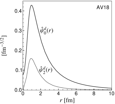
Figure 12: Deuteron wave function: $\hat{\psi}^{d}_{0}(r)$ and $\hat{\psi}^{d}_{2}(r)$ for the Bonn-A (left) and the Argonne V18 (right) interaction. There is a noticeable difference in the $d$-wave admixture, the Argonne V18 interaction has stronger tensor correlations. The behavior of the wave function at the origin shows a larger correlation hole caused by the stronger repulsive core of the Argonne V18 as compared to that of the Bonn-A interaction.

The correlations due to the repulsive core express themselves as a depletion of the relative wave functions at distances below $1\;\mathrm{fm}$. This correlation hole will be created by the unitary radial shift operator ${c}_{r}^{\phantom{\dagger}}$ as explained in section 4.1.

The correlation between spins and relative orientation of the nucleons due to the tensor force is contained in the admixture of a $d$-wave component $\hat{\psi}^{d}_{2}(r)\big{|}\,{(21)1M}\,\big{>}$, where the orbital angular momentum $L=2$ is coupled with the spin $S=1$ to the total angular momentum $J=1$. In Fig. 13 the two-body density

$$\hat{\rho}^{(2)}_{1M_{S}}(\boldsymbol{{r}})=\frac{1}{3}\sum^{1}_{M=-1}\left|\big{<}\,{\boldsymbol{{r}};S=1,M_{S}}\,\big{|}\,{\hat{d};1M}\,\big{>}\right|^{2}$$ (63)

is displayed. It is the projection of the deuteron on the $S=1,M_{S}$ component, averaged over all directions. Both, the correlation hole in the center and the alignment of the spatial density with the spin direction are clearly visible. Those proton-neutron pairs which have parallel spins, i.e. $M_{S}=1$, are located at the “north” and “south” poles so that their relative distance vector $\boldsymbol{{r}}$ is aligned with their spins. Pairs with opposite spin, i.e. $M_{S}=0$, are found around the “equator” where their spins are perpendicular to $\boldsymbol{{r}}$. This is exactly the pattern one expects for the interaction of two magnetic dipoles.

Figure 13: Surfaces of constant density in the deuteron ($\rho^{(2)}_{1M_{S}}=0.005\mathrm{fm}^{-3}$) for $M_{S}=\pm 1$ on the left and $M_{S}=0$ on the right. The plots are done for the Argonne V18 interaction.

A single Slater determinant, where the spin direction of a single particle state depends at most on the position $\boldsymbol{{r}}_{i}$ and not on the relative coordinate $\boldsymbol{{r}}_{ij}=\boldsymbol{{r}}_{i}-\boldsymbol{{r}}_{j}$ of two nucleons, cannot reflect the correlations between spins and relative orientation of the nucleons. We face a similar problem as with the short-range correlations. A single Slater determinant does not have the proper degrees of freedom needed for the description of the physical system. Since Slater determinants form a complete basis the appropriate state can always be written as a superposition of determinants. One needs however a huge number of those for a successful description. For example in second order perturbation theory the tensor interaction scatters to intermediate states with energies of about $300\;\mathrm{MeV}$ which would mean that about $30\hbar\omega$ excitations have to be included in shell-model calculations [22].

Our aim is, as with the short-range correlations, to include these tensor correlations into the many-body state by means of a unitary correlation operator ${C}_{\Omega}^{\phantom{\dagger}}$. The form of the generator is, however, not self-evident because one needs to correlate the spins of the nucleons with the relative orientation of the nucleons.

To define our unitary tensor correlator we start with an ansatz $\big{|}\,{d;1M}\,\big{>}$ for the uncorrelated deuteron state that has only an $L=0$ component.

$$\big{<}\,{r}\,\big{|}\,{d;1M}\,\big{>}=\psi^{d}_{0}(r)\big{|}\,{(01)1M}\,\big{>}$$ (64)

Here we imply that $\psi^{d}_{0}(r)$ already includes the radial correlations.

We require that the tensor correlator ${c}_{\Omega}^{\phantom{\dagger}}$ generates the $L=2$ component of the correlated deuteron state by mapping the uncorrelated $\big{|}\,{d;1M}\,\big{>}$ onto the exact solution $\big{|}\,{\hat{d};1M}\,\big{>}$

$$\big{|}\,{\hat{d};1M}\,\big{>}={c}_{\Omega}^{\phantom{\dagger}}\big{|}\,{d;1M}\,\big{>}=\exp\{-\mathrm{i}{g}_{\Omega}\}\big{|}\,{d;1M}\,\big{>}\;.$$ (65)

The generator ${g}_{\Omega}$ has to be a scalar operator with respect to rotations as the quantum numbers $J,M$ of the total angular momentum are not changed. In coordinate space it has to be a tensor operator of rank two, there is no other possibility to connect $L=0$ with $L=2$ states. If it is of rank two in coordinate space it also has to be of rank two in spin space. In the two-body spin space there is only one tensor of rank two so that only the coordinate space part needs to be specified. We restrict the choice by demanding that the correlator should make shifts only perpendicular to the relative orientation of the nucleons because radial shifts are already treated by the radial correlator. In order to achieve these shifts we use the orbital momentum operator $\boldsymbol{{p}}_{\Omega}$, defined in Eq. (42), to construct the following tensor

$$s_{\!12}(\boldsymbol{{r}},\boldsymbol{{p}}_{\Omega})=\frac{3}{2}\Bigl{(}(\boldsymbol{{\sigma}}_{1}\!\cdot\!\boldsymbol{{p}}_{\Omega})(\boldsymbol{{\sigma}}_{2}\!\cdot\!\boldsymbol{{r}})+(\boldsymbol{{\sigma}}_{1}\!\cdot\!\boldsymbol{{r}})(\boldsymbol{{\sigma}}_{2}\!\cdot\!\boldsymbol{{p}}_{\Omega})\Bigr{)}$$ (66)

and the generator ${g}_{\Omega}$ for spin-dependent tangential shifts as

$${g}_{\Omega}=\vartheta(r)s_{\!12}(\boldsymbol{{r}},\boldsymbol{{p}}_{\Omega})\;.$$ (67)

This operator has indeed all the required properties. It is a scalar operator of rank two both in coordinate and spin-space. It does not shift the relative wave function radially because $s_{\!12}(\boldsymbol{{r}},\boldsymbol{{p}}_{\Omega})$ commutes with ${r}=|\boldsymbol{{r}}|$. This can be shown by using the commutator relation

$$\bigl{[}\,{p}_{\Omega k}\,,{r}_{l}\,\bigr{]}=\mathrm{i}\left(\frac{{r}_{k}{r}_{l}}{r^{2}}-\delta_{kl}\right)\;,$$ (68)

where $k,l$ denote the three spatial directions. With Eq. (68) it is also easy to proof that $s_{\!12}(\boldsymbol{{r}},\boldsymbol{{p}}_{\Omega})$ is hermitean and symmetric under particle exchange.

The strength of the tensor correlation can be adjusted with the tensor correlation function $\vartheta(r)$ for each distance $r$ independently. Like the shift function $s(r)$ in the case of radial correlations, $\vartheta(r)$ will depend on the potential and on the system under investigation.

It is very illustrative to look at the generator ${g}_{\Omega}$ in angular momentum representation. The angular and spin dependence of ${g}_{\Omega}$ is contained in the $s_{\!12}(\boldsymbol{{r}},\boldsymbol{{p}}_{\Omega})$ operator. The calculation of its matrix elements is outlined in appendix A.2. We notice that all diagonal matrix elements are zero. The operator $s_{\!12}(\boldsymbol{{r}},\boldsymbol{{p}}_{\Omega})$ and therefore also the generator ${g}_{\Omega}$ only connects states with $L-L^{\prime}=\pm 2$ and the same total angular momentum $J,M$. For example in the $J=1$ subspace the matrix elements of $s_{\!12}(\boldsymbol{{r}},\boldsymbol{{p}}_{\Omega})$ are

$s_{\!12}(\boldsymbol{{r}},\boldsymbol{{p}}_{\Omega})$	$\big{|}\,{(01)1}\,\big{>}$	$\big{|}\,{(11)1}\,\big{>}$	$\big{|}\,{(21)1}\,\big{>}$
$\big{<}\,{(01)1}\,\big{|}$	$0$	$0$	$-3\mathrm{i}\sqrt{2}$
$\big{<}\,{(11)1}\,\big{|}$	$0$	$0$	$0$
$\big{<}\,{(21)1}\,\big{|}$	$3\mathrm{i}\sqrt{2}$	$0$	$0$

Using these matrix elements we can immediately write the correlated deuteron wave function as

$$\big{<}\,{r}\,\big{|}\,{{c}_{\Omega}^{\phantom{\dagger}}}\,\big{|}\,{d;1M}\,\big{>}=\big{<}\,{r}\,\big{|}\,{\exp\bigl{\{}-\mathrm{i}\,\vartheta^{d}(r)s_{\!12}(\boldsymbol{{r}},\boldsymbol{{p}}_{\Omega})\bigr{\}}}\,\big{|}\,{d;1M}\,\big{>}=\\ \psi^{d}_{0}(r)\Bigl{[}\,\cos\!\left(3\sqrt{2}\,\vartheta^{d}(r)\right)\big{|}\,{(01)1M}\,\big{>}+\sin\!\left(3\sqrt{2}\,\vartheta^{d}(r)\right)\big{|}\,{(21)1M}\,\big{>}\,\Bigr{]}\;.$$ (69)

When we compare this to the exact deuteron solution Eq. (62) we find the deuteron correlation function

$$\vartheta^{d}(r)=\frac{1}{3\sqrt{2}}\arctan\frac{\hat{\psi}^{d}_{2}(r)}{\hat{\psi}^{d}_{0}(r)}\;.$$ (70)

The deuteron correlation functions $\vartheta^{d}(r)$ for the Bonn-A and the Argonne V18 potential are shown in Fig. 14. The correlations are stronger in case of the Argonne V18 interaction at short distances and show a different behavior for $r\rightarrow 0$ indicating the stronger tensor force in the AV18 potential.

Figure 14: Deuteron correlation functions $\vartheta^{d}(r)$ for the Bonn-A and Argonne V18 interactions.

The uncorrelated deuteron trial state Eq. (64) has no $L=2$ admixture at all. Thus the deuteron correlator which maps the trial state onto the exact deuteron solution has to generate the entire radial wave function $\hat{\psi}^{d}_{2}(r)$. The correlator is therefore very long ranged and will induce three- and higher-body correlations in many-body states. In order to avoid the higher-body terms one should not put all responsibility for creating long-ranged or low-momentum $L=2$ admixtures on the correlator, but should include those into the degrees of freedom of the uncorrelated many-body trial state. Only the short-range or high-momentum part of the tensor correlations should be taken care of by the correlator ${C}_{\Omega}^{\phantom{\dagger}}$. Such a correlator can then be used efficiently in many-body calculations because the two-body approximation is valid when the correlation range is short enough.

In the discussion of tensor correlations in the deuteron the radial correlations have not been considered explicitly but were already included in the “tensor-uncorrelated” state $\big{|}\,{d;1M}\,\big{>}$. In the following sections we combine both correlations.

4.3 Correlated operators in coordinate space representation

Using the unitarity of ${c}_{r}^{\phantom{\dagger}}$ and the transformation properties (47) it is easy to see that

$${c}_{r}^{\dagger}\,{\boldsymbol{{p}}}_{\Omega}\,{c}_{r}^{\phantom{\dagger}}=\frac{r}{R_{+}(r)}\ {\boldsymbol{{p}}}_{\Omega}\qquad\mathrm{and}\qquad{c}_{r}^{\dagger}\,s_{\!12}(\boldsymbol{{r}},\boldsymbol{{p}}_{\Omega})\,{c}_{r}^{\phantom{\dagger}}=s_{\!12}(\boldsymbol{{r}},\boldsymbol{{p}}_{\Omega})\;.$$ (71)

From that follows immediately that the radially correlated tensor correlator

$${c}_{r}^{\dagger}{c}_{\Omega}^{\phantom{\dagger}}{c}_{r}^{\phantom{\dagger}}={c}_{r}^{\dagger}\exp\bigl{\{}-\mathrm{i}\,\vartheta(r)s_{\!12}(\boldsymbol{{r}},\boldsymbol{{p}}_{\Omega})\bigr{\}}{c}_{r}^{\phantom{\dagger}}=\exp\bigl{\{}-\mathrm{i}\,\vartheta(R_{+}(r))s_{\!12}(\boldsymbol{{r}},\boldsymbol{{p}}_{\Omega})\bigr{\}}$$ (72)

differs only by a transformed radial dependence of the tensor correlation function $\vartheta(r)$. The technical advantage of unitary correlations is quite obvious in this example.

For tensor correlated operators

$${c}_{\Omega}^{\dagger}\,{a}\,{c}_{\Omega}^{\phantom{\dagger}}=e^{\mathrm{i}{g}_{\Omega}}\,{a}\,e^{-\mathrm{i}{g}_{\Omega}}$$ (73)

it is no longer possible to give a closed form for the most general operator ${a}$ in coordinate representation. We can use the Baker-Campbell-Hausdorff formula

$$\begin{split}{c}_{\Omega}^{\dagger}\,{a}\,{c}_{\Omega}^{\phantom{\dagger}}&={a}+\mathrm{i}\bigl{[}{{g}_{\Omega}},{{a}}\bigr{]}_{-}+\frac{i^{2}}{2}\bigl{[}{{g}_{\Omega}},{\bigl{[}{{g}_{\Omega}},{{a}}\bigr{]}_{-}}\bigr{]}_{-}+\ldots\\ &=e^{\mathsf{L}_{\Omega}}{a}\;,\end{split}$$ (74)

and the superoperator $\mathsf{L}_{\Omega}=\mathrm{i}\,\bigl{[}{{g}_{\Omega}},{\circ}\bigr{]}_{-}$ to evaluate the expression in two-body space. In the case of the Hamilton operator for example we have to to evaluate the repeated application of $\mathsf{L}_{\Omega}$ on the kinetic energy and all components of the potential.

The tensor correlation of the radial momentum ${p}_{r}$ and distance ${r}$ are special cases where the power series (74) terminates

$$\begin{split}{c}_{\Omega}^{\dagger}\,{r}{c}_{\Omega}^{\phantom{\dagger}}&={r}\\ {c}_{\Omega}^{\dagger}\,{p}_{r}{c}_{\Omega}^{\phantom{\dagger}}&={p}_{r}-\vartheta^{\prime}(r)s_{\!12}(\boldsymbol{{r}},\boldsymbol{{p}}_{\Omega})\;.\end{split}$$ (75)

$\vartheta^{\prime}(r)$ denotes the first derivative of $\vartheta(r)$. With Eq. (75) the tensor correlated radial kinetic energy is readily calculated as

$$\begin{split}{c}_{\Omega}^{\dagger}\,\frac{{p}_{r}^{2}}{m}{c}_{\Omega}^{\phantom{\dagger}}&=\frac{1}{m}\bigl{(}{p}_{r}-\vartheta^{\prime}(r)s_{\!12}(\boldsymbol{{r}},\boldsymbol{{p}}_{\Omega})\bigr{)}^{2}\\ &=\frac{{p}_{r}^{2}}{m}-\bigl{(}{p}_{r}\vartheta^{\prime}(r)+\vartheta^{\prime}(r){p}_{r}\bigr{)}s_{\!12}(\boldsymbol{{r}},\boldsymbol{{p}}_{\Omega})+\bigl{(}\vartheta^{\prime}(r)\bigr{)}^{2}s_{\!12}(\boldsymbol{{r}},\boldsymbol{{p}}_{\Omega})^{2}\;,\end{split}$$ (76)

where $s_{\!12}(\boldsymbol{{r}},\boldsymbol{{p}}_{\Omega})^{2}$ can also be written as (see Eqs. (156) and (157))

$$s_{\!12}(\boldsymbol{{r}},\boldsymbol{{p}}_{\Omega})^{2}=9\ \bigl{(}{\boldsymbol{{s}}}^{2}+3\ \boldsymbol{{l}}\!\cdot\!\boldsymbol{{s}}+(\boldsymbol{{l}}\!\cdot\!\boldsymbol{{s}})^{2}\bigr{)}\;.$$ (77)

One sees that the tensor correlation creates again structures that exist already in the potential, see Eq. (9).

For other parts of the interaction, like the spin-orbit $\boldsymbol{{l}}\!\cdot\!\boldsymbol{{s}}$ or the tensor one $s_{\!12}(\hat{\boldsymbol{{r}}},\hat{\boldsymbol{{r}}})$, the power series (74) does not terminate but results in ever higher powers of angular momentum and tensor operators. The coordinate space representation is discussed in [11] and will be pursued further in a forthcoming paper. As it is no longer possible to give closed expressions for the most general tensor correlated operator ${c}_{\Omega}^{\dagger}{a}{c}_{\Omega}^{\phantom{\dagger}}$ in coordinate representation, in the following sections we shall use the angular momentum representation where it is easy to state explicitly the correlated states and correlated interaction.

4.4 Tensor correlated angular momentum eigenstates

The action of the tensor correlator can be evaluated explicitly in two-body angular momentum eigenstates $\left|(LS)JM\right>$ that are used for example in shell-model calculations. The operator $s_{\!12}(\boldsymbol{{r}},\boldsymbol{{p}}_{\Omega})$ is a scalar two-body operator that is a tensor of rank two in coordinate and spin space. Therefore it connects only states with the same total angular momentum $J,M$ and spin $S=1$. In addition it is constructed to have only off-diagonal matrix elements for $|L^{\prime}-L|=2$ so that for each $J$-subspace it is only a $2\times 2$ matrix and thus easy to exponentiate.

The matrix elements of $s_{\!12}(\boldsymbol{{r}},\boldsymbol{{p}}_{\Omega})$ are (see App. A.2.4)

$$\big{<}\,{(L^{\prime}S^{\prime})J^{\prime}M^{\prime}}\,\big{|}\,{s_{\!12}(\boldsymbol{{r}},\boldsymbol{{p}}_{\Omega})}\,\big{|}\,{(LS)JM}\,\big{>}=\\ \mathrm{i}\,3\,\sqrt{J(J+1)}\bigl{(}\delta_{L^{\prime},J+1}\delta_{L,J-1}-\delta_{L^{\prime}\!,J-1}\delta_{L,J+1}\bigr{)}\delta_{S^{\prime}\!,1}\delta_{S,1}\delta_{J^{\prime}\!,J}\delta_{M^{\prime}\!,M}\;.$$ (78)

For the sake of convenience we introduce the angle

$$\theta^{(J)}(r)=3\,\sqrt{J(J+1)}\,\vartheta(r)\;.$$ (79)

With (78) and (79) states with $L=J\mp 1$ are tensor correlated as

$${c}_{\Omega}^{\phantom{\dagger}}\big{|}\,{(J\!\mp\!1,1)JM}\,\big{>}=\\ \cos\bigl{(}\theta^{(J)}(r)\bigr{)}\big{|}\,{(J\!\mp\!1,1)JM}\,\big{>}\pm\sin\bigl{(}\theta^{(J)}(r)\bigr{)}\big{|}\,{(J\!\pm\!1,1)JM}\,\big{>}\;,$$ (80)

while states with $L=J$ remain unchanged for both, $S=0$ and $S=1$,

$${c}_{\Omega}^{\phantom{\dagger}}\big{|}\,{(JS)JM}\,\big{>}=\big{|}\,{(JS)JM}\,\big{>}\;.$$ (81)

4.5 Correlated operators in angular momentum representation

For the evaluation of two-body matrix elements it is more convenient to work with radially correlated operators and tensor correlated states. Therefore we make use of the unitarity of the radial correlation operator ${c}_{r}^{\phantom{\dagger}}$ and evaluate correlated two-body matrix elements as

$$\big{<}\,{\phi}\,\big{|}\,{{c}_{r}^{\dagger}{c}_{\Omega}^{\dagger}{a}{c}_{\Omega}^{\phantom{\dagger}}{c}_{r}^{\phantom{\dagger}}}\,\big{|}\,{\psi}\,\big{>}=\big{<}\,{\phi}\,\big{|}\,{({c}_{r}^{\dagger}{c}_{\Omega}^{\phantom{\dagger}}{c}_{r}^{\phantom{\dagger}})^{\dagger}({c}_{r}^{\dagger}{a}{c}_{r}^{\phantom{\dagger}})({c}_{r}^{\dagger}{c}_{\Omega}^{\phantom{\dagger}}{c}_{r}^{\phantom{\dagger}})}\,\big{|}\,{\psi}\,\big{>}\;.$$ (82)

Using this trick radially correlated operators ${c}_{r}^{\dagger}{a}{c}_{r}^{\phantom{\dagger}}$ can be used in tensor correlated states which are uncorrelated with respect to the short-range repulsion.

All operators considered in the following are scalar, hence they are diagonal in $J,M$ and their matrixelements do not depend on the magnetic quantum numbers $M=-J,\ldots,J$. Therefore we will omit $M$ and write only $\big{|}\,{(LS)J}\,\big{>}$. The isospin quantum numbers $T,M_{T}$ are omitted as well.

As a consequence of Eq. (81) the interaction in the states $\big{|}\,{(JS)J}\,\big{>}$ will not be influenced by the tensor correlations

$$\big{<}\,{(JS)J}\,\big{|}\,{{c}_{r}^{\dagger}{c}_{\Omega}^{\dagger}{h}{c}_{\Omega}^{\phantom{\dagger}}{c}_{r}^{\phantom{\dagger}}}\,\big{|}\,{(JS)J}\,\big{>}=\big{<}\,{(JS)J}\,\big{|}\,{{c}_{r}^{\dagger}{h}{c}_{r}^{\phantom{\dagger}}}\,\big{|}\,{(JS)J}\,\big{>}\;.$$ (83)

The diagonal matrix elements of the two-body radial kinetic energy that is fully correlated are calculated using Eqs. (52) and (76) as

$$\big{<}\,{(J\!\mp\!1,1)J}\,\big{|}\,{{\hat{t}}^{[2]}_{r}}\,\big{|}\,{(J\!\mp\!1,1)J}\,\big{>}=\\ \begin{split}&=\big{<}\,{(J\!\mp\!1,1)J}\,\big{|}\,{{c}_{r}^{\dagger}{c}_{\Omega}^{\dagger}{t}_{r}{c}_{\Omega}^{\phantom{\dagger}}{c}_{r}^{\phantom{\dagger}}-{t}_{r}}\,\big{|}\,{(J\!\mp\!1,1)J}\,\big{>}\\ &=\frac{1}{2}\biggl{[}p_{r}^{2}\frac{1}{2\hat{\mu}_{r}(r)}+\frac{1}{2\hat{\mu}_{r}(r)}p_{r}^{2}\biggr{]}+\frac{J(J+1)}{m}\Bigl{(}3\,\vartheta^{\prime}(R_{+}(r))\Bigr{)}^{2}+\hat{w}(r)\;.\end{split}$$ (84)

The contribution from the tensor correlation is a centrifugal-like term originating from the radial dependence of the tensor correlation function. “Radial mass” $\hat{\mu}_{r}(r)$ and potential term $\hat{w}(r)$ are unchanged from Eq. (53) and (54).

The mixture of different angular momenta by the tensor correlator leads to the following fully correlated kinetic energy of the orbital motion in the two-body system

$$\big{<}\,{(J\!\mp\!1,1)J}\,\big{|}\,{{\hat{t}}^{[2]}_{\Omega}}\,\big{|}\,{(J\!\mp\!1,1)J}\,\big{>}=\big{<}\,{(J\!\mp\!1,1)J}\,\big{|}\,{{c}_{r}^{\dagger}{c}_{\Omega}^{\dagger}{t}_{\Omega}{c}_{\Omega}^{\phantom{\dagger}}{c}_{r}^{\phantom{\dagger}}-{t}_{\Omega}}\,\big{|}\,{(J\!\mp\!1,1)J}\,\big{>}=\\ \begin{aligned} =\frac{1}{m(R_{+}(r))^{2}}\Bigl{\{}&\cos^{2}\bigl{(}\theta^{(J)}(R_{+}(r))\bigr{)}\big{<}\,{(J\!\mp\!1,1)J}\,\big{|}\,{\boldsymbol{{l}}^{2}}\,\big{|}\,{(J\!\mp\!1,1)J}\,\big{>}\\ &+\sin^{2}\bigl{(}\theta^{(J)}(R_{+}(r))\bigr{)}\big{<}\,{(J\!\pm\!1,1)J}\,\big{|}\,{\boldsymbol{{l}}^{2}}\,\big{|}\,{(J\!\pm\!1,1)J}\,\big{>}\Bigr{\}}\\ -\frac{1}{mr^{2}}&\big{<}\,{(J\!\mp\!1,1)J}\,\big{|}\,{\boldsymbol{{l}}^{2}}\,\big{|}\,{(J\!\mp\!1,1)J}\,\big{>}\;.\end{aligned}$$ (85)

The central potentials ${v}^{c}=v^{c}({r})$ are not affected by the tensor correlations

$$\big{<}\,{(J\!\mp\!1,1)J}\,\big{|}\,{{c}_{r}^{\dagger}{c}_{\Omega}^{\dagger}{v}^{c}{c}_{\Omega}^{\phantom{\dagger}}{c}_{r}^{\phantom{\dagger}}}\,\big{|}\,{(J\!\mp\!1,1)J}\,\big{>}=v^{c}(R_{+}(r))\;.$$ (86)

Like the above terms the spin-orbit interaction ${v}^{b}=v^{b}(r)\>\boldsymbol{{l}}\!\cdot\!\boldsymbol{{s}}$ has only diagonal contributions from the distinct $L$ channels of the correlated states have to be considered

$$\big{<}\,{(J\!\mp\!1,1)J}\,\big{|}\,{{c}_{r}^{\dagger}{c}_{\Omega}^{\dagger}{v}^{b}{c}_{\Omega}^{\phantom{\dagger}}{c}_{r}^{\phantom{\dagger}}}\,\big{|}\,{(J\!\mp\!1,1)J}\,\big{>}=\\ \begin{aligned} =v^{b}(R_{+}(r))\>\Bigl{\{}&\cos^{2}\bigl{(}\theta^{(J)}(R_{+}(r))\bigr{)}\>\big{<}\,{(J\!\mp\!1,1)J}\,\big{|}\,{\boldsymbol{{l}}\!\cdot\!\boldsymbol{{s}}}\,\big{|}\,{(J\!\mp\!1,1)J}\,\big{>}\\ &+\sin^{2}\bigl{(}\theta^{(J)}(R_{+}(r))\bigr{)}\>\big{<}\,{(J\!\pm\!1,1)J}\,\big{|}\,{\boldsymbol{{l}}\!\cdot\!\boldsymbol{{s}}}\,\big{|}\,{(J\!\pm\!1,1)J}\,\big{>}\Bigr{\}}\;.\end{aligned}$$ (87)

The matrix elements of the correlated tensor interactions ${v}^{t}=v^{t}(r)\>s_{\!12}(\hat{\boldsymbol{{r}}},\hat{\boldsymbol{{r}}})$ also include contributions from the off-diagonal matrix elements between the $L$ channels of the correlated state

$$\big{<}\,{(J\!\mp\!1,1)J}\,\big{|}\,{{c}_{r}^{\dagger}{c}_{\Omega}^{\dagger}{v}^{t}{c}_{\Omega}^{\phantom{\dagger}}{c}_{r}^{\phantom{\dagger}}}\,\big{|}\,{(J\!\mp\!1,1)J}\,\big{>}=\\ \begin{aligned} v^{t}&(R_{+}(r))\>\Bigl{\{}\cos^{2}\bigl{(}\theta^{(J)}(R_{+}(r))\bigr{)}\>\big{<}\,{(J\!\mp\!1,1)J}\,\big{|}\,{s_{\!12}(\hat{\boldsymbol{{r}}},\hat{\boldsymbol{{r}}})}\,\big{|}\,{(J\!\mp\!1,1)J}\,\big{>}\\ &\pm 2\cos\bigl{(}\theta^{(J)}(R_{+}(r))\bigr{)}\sin\bigl{(}\theta^{(J)}(R_{+}(r))\bigr{)}\>\big{<}\,{(J\!\mp\!1,1)J}\,\big{|}\,{s_{\!12}(\hat{\boldsymbol{{r}}},\hat{\boldsymbol{{r}}})}\,\big{|}\,{(J\!\pm\!1,1)J}\,\big{>}\\ &+\sin^{2}\bigl{(}\theta^{(J)}(R_{+}(r))\bigr{)}\>\big{<}\,{(J\!\pm\!1,1)J}\,\big{|}\,{s_{\!12}(\hat{\boldsymbol{{r}}},\hat{\boldsymbol{{r}}})}\,\big{|}\,{(J\!\pm\!1,1)J}\,\big{>}\Bigr{\}}\;.\end{aligned}$$ (88)

The calculation of matrix elements that are off-diagonal in angular momentum is straightforward using Eqs. (80,81).

5 Bonn-A and Argonne-V18 correlators

5.1 Choice of correlation functions

In this section we discuss the choice of the correlation functions $R_{+}(r)$ and $\vartheta(r)$. We use two general concepts: minimizing the ground state energy and mapping of uncorrelated onto exact eigenstates of the Hamiltonian. Both will yield very similar answers.

The ansatz for the correlated many-body state

$$\big{|}\,{\hat{\Psi}}\,\big{>}={C}\big{|}\,{\Psi}\,\big{>}={C}_{\Omega}^{\phantom{\dagger}}{C}_{r}^{\phantom{\dagger}}\big{|}\,{\Psi}\,\big{>}$$ (89)

consists of the uncorrelated state $\big{|}\,{\Psi}\,\big{>}$ and the correlation operator ${C}$. Both contain degrees of freedom that can be varied to find the minimum in the energy

$$\big{<}\,{\Psi}\,\big{|}\,{{{{C}}}^{{\dagger}}{H}{C}}\,\big{|}\,{\Psi}\,\big{>}=\mbox{min}\;.$$ (90)

In $\big{|}\,{\Psi}\,\big{>}$ they are for example the single-particle states or in case of a superposition of Slater determinants also their coefficients. After having defined the operator structure of ${C}_{\Omega}^{\phantom{\dagger}}$ and ${C}_{r}^{\phantom{\dagger}}$ the remaining freedom is to choose the correlation functions $R_{+}(r)$ and $\vartheta(r)$. In principle one could do a functional variation in (90) for each nucleus to find the optimal correlation functions. In practice we parametrize $R_{+}(r)$ and $\vartheta(r)$ and vary only a few parameters.

The other method is to map a typical uncorrelated two-body state at short distances onto the exact solution. Let us define the exact eigenvalue problem by

$$H\big{|}\,{\hat{\Psi}_{n}}\,\big{>}=E_{n}\big{|}\,{\hat{\Psi}_{n}}\,\big{>}$$ (91)

with the exact eigenstates $\big{|}\,{\hat{\Psi}_{n}}\,\big{>}$. The task of ${C}$ is to map the energetically lowest uncorrelated states as well as possible onto the exact eigenstates

$${C}\big{|}\,{\Psi_{n}}\,\big{>}\approx\big{|}\,{\hat{\Psi}_{n}}\,\big{>}\;.$$ (92)

As the structure of ${C}$ is given, up to the radial dependences $R_{+}(r)$ and $\vartheta(r)$, in general one representative state $\big{|}\,{\Psi_{n}}\,\big{>}$ in each spin isospin channel is sufficient to determine those. The physical idea is that the momentum distributions of the uncorrelated trial states reside in the low momentum regime, while the short range correlations create high momentum components that are more or less independent of the long range behaviour described by $\big{|}\,{\Psi_{n}}\,\big{>}$. For the radial correlations this is demonstrated in Fig. 9. It is obvious that ${C}$ as defined in the previous sections cannot fulfill Eq. (92) for all $n$ exactly but it should make the off-diagonal matrix elements $\big{<}\,{\Psi_{k}}\,\big{|}{{{C}}}^{{\dagger}}H{C}\big{|}\,{\Psi_{n}}\,\big{>}$ of the correlated Hamiltonian much smaller than $\big{<}\,{\Psi_{k}}\,\big{|}H\big{|}\,{\Psi_{n}}\,\big{>}$ of the bare one.

In the uncorrelated many-body states of shell-model or mean-field configurations two-body states for the relative motion with the lowest relative angular momenta and relative momenta have the biggest weight. Therefore the correlators will be determined in the lowest angular momentum states of the respective spin and isospin channels at zero or ground state energy. The influence of the correlations decreases with increasing relative orbital angular momentum $L$ as the centrifugal barrier suppresses significantly already the uncorrelated two-body density at short distances.

In the $S,T=0,0$ and the $S,T=0,1$ channels where we do not have to deal with tensor correlations the correlators are therefore fixed with $\big{|}\,{(10)1;0}\,\big{>}$ and $\big{|}\,{(00)0;1}\,\big{>}$ trial states. In the $S,T=1,0$ channel our uncorrelated trial state will be $\big{|}\,{(01)1;0}\,\big{>}$. The tensor correlator will admix the $\big{|}\,{(21)1;0}\,\big{>}$ state. In the $S,T=1,1$ channel the situation is more complicated. The lowest orbital angular momentum $L=1$ can be coupled with the spin $S=1$ to the total angular momenta $J=0,1,2$. Only for $J=2$ we have to deal with tensor correlations which will admix $\big{|}\,{(31)2;1}\,\big{>}$ states.

Following these principles we will determine now the radial and tensor correlators for the Bonn-A and the Argonne V18 interaction. By comparing the correlators side-by-side a better understanding of common and specific properties of the different nuclear interactions and the correlations can be achieved.

The Argonne V8’ interaction is by construction identical to the Argonne V18 interaction in the lowest $L$ channels. As we fix our correlators in these channels the Argonne V18 correlators presented are identical to the Argonne V8’ correlators.

Correlators that minimize the energy of the many-body system will only be given for the $\@@nuc{4}{He}$ nucleus. For heavier nuclei like $\@@nuc{16}{O}$ and $\@@nuc{40}{Ca}$ they turn out to be nearly indistinguishable from the two-body optimized correlators. This shows that the short range correlations are essentially independent of the size of the many-body system. The nuclear saturation property limits the largest possible density so that adding more nucleons has negligible effect on short range correlations between two nucleons. This is in accord with the findings of Ref. [23] where the short-range tensor structure of the deuteron is also found in heavier nuclei.

The correlation functions determined from mapping the lowest energy eigenstate in the two-body system will not be used in many-body calculations but are shown in the graphs for comparison. Those resulting from minimizing energies are parametrized in the style of the ones obtained by mapping the uncorrelated states on the exact eigenstates. The form and the three or four parameters which determine the parametrized correlation functions are summarized in Appendix C.

5.2 $S=0,T=1$ channel

Figure 15: Radial correlations in the $S,T=0,1$ channel for the Bonn-A (left hand side) and the Argonne V18 interaction (right hand side). In the upper part $\psi_{0}^{\mathit{min}}(r)$ is obtained by minimizing the energy with the constant trial function $\varphi_{0}(r)=\mathit{const}$. Mapping a Gaussian trial function onto the zero-energy scattering solution as displayed in the insets of the upper part defines the correlation function labelled “$\mathit{zero}$”. Applying this correlator to the constant trial function $\varphi_{0}(r)$ results in $\psi_{0}^{\mathit{zero}}(r)$. The correlation functions are displayed in the lower part together with the $\@@nuc{4}{He}$ optimized correlation function.

In the $S,T=0,1$ channel, where we do not have to deal with tensor correlations, the radial correlators are fixed with the zero-energy scattering state $\big{|}\,{k=0;(00)0;1}\,\big{>}$ state with $L=0$. We obtain the correlators labelled “$\mathit{zero}$” from the mapping of a Gaussian trial function onto the scattering solution and the correlators labeled “$\mathit{min}$” by minimizing the energy in the two-body system with a constant trial function [12]. The resulting correlated radial wave functions are shown in the upper part of Fig. 15 and the corresponding radial correlation functions in the lower part. In addition we determine a correlator optimized for the $\@@nuc{4}{He}$ nucleus in two-body approximation. Here we use a harmonic oscillator shell-model trial state which reproduces the experimental radius of the $\@@nuc{4}{He}$ nucleus. All three correlators turn out to be very similar indicating that in this channel there is little ambiguity in separating the short range from the long range behaviour or the high momentum from the low momentum content in the relative motion.

Comparing the Bonn with the Argonne correlator we observe however considerable differences. The depletion of the Argonne scattering solution at small distances $r$ is much stronger than in case of the Bonn potential. The correlation functions of the Argonne interaction are correspondingly stronger but of the same range as the Bonn correlation functions.

5.3 $S=1,T=0$ channel

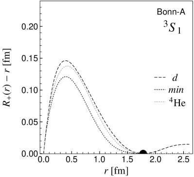
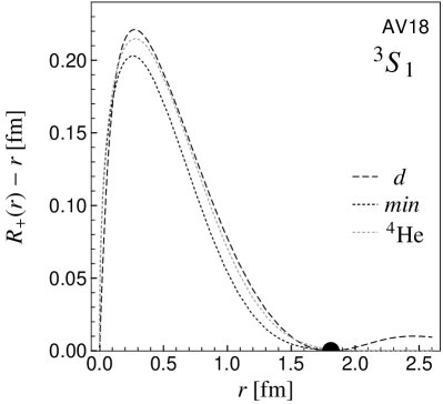
Figure 16: Radial correlation functions $R_{+}(r)$ in the $S,T=1,0$ channel for Bonn-A interaction (left) and the Argonne AV18 interaction (right). Applying the radial correlation functions labelled “$\mathit{min}$” and “$d$” to the constant trial function $\varphi_{0}(r)=\mathit{const}$ results in $\psi^{\mathit{min}}_{0}(r)$ and $\psi^{d}_{0}(r)$, respectively. In the insets the mapping of the Gaussian trial function onto the “tensor-decorrelated” deuteron solution ${c}_{r}\phi^{d}_{0}(r)=\psi^{d}_{0}(r)=\sqrt{\hat{\psi}^{d}_{0}(r)^{2}+\hat{\psi}^{d}_{2}(r)^{2}}$ is indicated. The radial correlation functions optimized for the $\@@nuc{4}{He}$ are shown in addition to the zero-energy scattering and the two-body optimized correlation functions in the lower part.

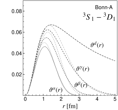
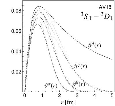
Figure 17: Tensor correlation functions for Bonn-A interaction (left hand side) and Argonne V18 interaction (right hand side). The tensor correlation functions $\alpha$, $\beta$ and $\gamma$ are the result of a minimization of the energy in the two-body system (black short-dashed lines) or in $\@@nuc{4}{He}$ trial state (gray short-dashed lines) with additional constraints on the range of the correlators.

In the $S,T=1,0$ channel the lowest energy state is the deuteron and thus we will use as uncorrelated trial state

$$\big{|}\,{d;(01)1;0}\,\big{>}\equiv\big{|}\,{d;(L=0,S=1)J=1,M;T=0,M_{T}=0}\,\big{>}\;.$$ (93)

As explained in detail in Sec. 4 we have to deal in this channel with radial and tensor correlations where the tensor correlator will admix an $L=2$ state.

The energy minimized correlators in the two-body system can be determined in principle by simultaneously minimizing the energy of a constant trial function $\varphi_{0}(r)=\mathit{const}$

$$\min_{R_{+}(r),\vartheta(r)}\big{<}\,{\varphi_{0};(01)1;0}\,\big{|}\,{{c}_{r}^{\dagger}{c}_{\Omega}^{\dagger}{h}{c}_{\Omega}^{\phantom{\dagger}}{c}_{r}^{\phantom{\dagger}}}\,\big{|}\,{\varphi_{0};(01)1;0}\,\big{>}$$ (94)

with respect to radial and tensor correlations and additional constraints concerning the correlation range in case of the tensor correlator. In practice we proceed in two steps. In the first step we determine the radial correlation function $R_{+}(r)$ using in Eq. (94) the deuteron tensor correlation function $\vartheta^{d}(r)$, given in Eq. (70). From the perspective of the radial correlator the long range behavior of the tensor correlator is not relevant. It therefore makes no real difference whether we use here the deuteron tensor correlator or a tensor correlator that has a restricted range. In a second step we vary the energy in the two-body system with respect to the tensor correlation function.

We proceed in the same way for the determination of the $\@@nuc{4}{He}$ optimized correlators, where the energy in a harmonic oscillator shell-model trial state is minimized with respect to radial and tensor correlators

$$\min_{R_{+}(r),\vartheta(r)}\big{<}\,{\@@nuc{4}{He}}\,\big{|}\,{\bigl{[}{C}_{r}^{\dagger}{C}_{\Omega}^{\dagger}{H}{C}_{\Omega}^{\phantom{\dagger}}{C}_{r}^{\phantom{\dagger}}\bigr{]}^{C2}}\,\big{|}\,{\@@nuc{4}{He}}\,\big{>}\;.$$ (95)

We end up with the radial correlators shown in Fig. 16. The mapping of a Gaussian trial function on the zero-energy scattering state is indicated in the insets of Fig. 16.

The radial correlation functions $R_{+}(r)$ obtained with the three methods turn out to be all very similar for the Bonn-A and the Argonne V18 interaction, respectively. But as in the other channels we can observe that the Argonne interaction induces stronger correlations, the correlation hole is deeper.

The naive idea to create the whole $L=2$ component only with the tensor correlator leads to an extremely long ranged correlation function that extends even outside the range of the interaction. This is of course in disaccord with the two-body approximation in the cluster expansion. Therefore we construct the tensor correlator by restricting the range of $\vartheta(r)$ to short distances, where the correlated states varies rapidly, and presume that the low momentum part of the $L=2$ state is represented in the uncorrelated trial state.

Tensor correlation functions $\vartheta^{\alpha,\beta,\gamma}(r)$ with limited range are obtained by minimizing the energy in the the-body system with the radially correlated $L=0$ trial state $\psi^{d}_{0}(r)$ under the constraint

$$\int\!\mathrm{d}{r}\;r^{2}\>\vartheta^{x}(r)\overset{!}{=}\begin{cases}0.1\,\mathrm{fm}^{3}&;\quad x=\alpha\\ 0.2\,\mathrm{fm}^{3}&;\quad x=\beta\\ 0.5\,\mathrm{fm}^{3}&;\quad x=\gamma\;.\end{cases}$$ (96)

The resulting correlation functions are displayed in Fig. 17 together with those obtained by minimizing the energy of the $\@@nuc{4}{He}$ trial state in the two-body approximation. Again both sets of correlation functions are very similar. Below $r\approx 1\,\mathrm{fm}$ they are almost unaffected by the limitation in range and even agree with the long ranged deuteron correlator. Comparing the Bonn-A and Argonne V18 interaction the influence of the stronger tensor part in the Argonne V18 is clearly visible. The tensor correlator for the zero-energy scattering solution is not shown because it is practically the same as the one obtained from the deuteron for distances below $2\,\mathrm{fm}$.

5.4 $S=0,T=0$ channel

Figure 18: Zero-energy scattering solutions and radial correlation functions in the $S,T=0,0$ channel for the Bonn-A interaction (left hand side) and the Argonne V18 interaction (right hand side). The $L=1$ trial state $\varphi_{1}(r)=r$ is mapped onto the zero-energy scattering solution $\psi^{\mathit{zero}}_{1}(r)={c}_{r}\varphi_{1}(r)$ with the correlation function $R_{+}^{\mathit{zero}}(r)$. Minimizing the energy in the two-body system with additional constraint on the correlation range leads to the correlation functions labelled “$\mathit{min}$”

According to our prescription we have to fix the correlator for the lowest angular momentum, which is $L=1$ in this channel and hence $J=1$. Both, the Bonn-A and the Argonne V18 interaction show a strong repulsion in the $S,T=0,0$ channel. This can be seen in the zero-energy scattering solutions $\psi^{\mathit{zero}}_{1}(r)$ plotted in the upper part of Fig. 18. We observe a remarkable difference in the Bonn-A and the Argonne V18 scattering solutions. Whereas the local Argonne interaction strongly suppresses the scattering solution at small distances the momentum dependent repulsion of the Bonn interaction shifts the wave function only for distances greater than about $0.5\,\mathrm{fm}$. This difference manifests itself also in the radial correlation functions $R_{+}^{\mathit{zero}}(r)$ derived from mapping the trial function $\varphi_{L=1}(r)=r$ onto the scattering solutions. The Argonne correlation function increases steeply for small $r$ whereas the Bonn correlation function starts to rise at greater distances as seen in the lower part of Fig. 18. The resulting correlation functions $R_{+}^{\mathit{zero}}(r)$ are extremely long ranged and cannot be used meaningfully in a many-body calculation.

By minimizing the energy with the trial function $\varphi_{1}(r)=r$ in the two-body system under the additional constraint

$$\int\!\mathrm{d}{r}\;r^{2}\>(R_{+}^{\mathit{min}}(r)-r)\overset{!}{=}0.1\,\mathrm{fm}^{3}$$ (97)

on the correlation range we obtain the correlators indicated by $\mathit{min}$ that have about the same range as the radial correlators in even channels. In the upper part of Fig. 18 their effect on the radially uncorrelated $\varphi_{1}(r)$ is compared to the zero-energy scattering solution $\psi^{\mathit{zero}}_{1}(r)$.

This odd channel does not occur in the $\@@nuc{4}{He}$ shell-model state. In many-body calculations of larger nuclei we will only present results obtained with the correlator $\mathit{min}$. Because of the small weight of the $S,T=0,0$ channel the final many-body results depend only very weakly on the particular choice of the radial correlation function in this channel.

5.5 $S=1,T=1$ channel

Figure 19: Radial correlation functions $R_{+}(r)$ in the $S,T=1,1$ channel for Bonn-A interaction (left hand side) and the Argonne V18 interaction (right hand side). The zero-energy scattering solution $\psi_{1}^{\mathit{zero}}(r)$ (dashed line) is calculated without the non-central parts of the interaction. $\varphi_{1}(r)=r$ is taken as the uncorrelated zero-energy scattering solution. The correlator which results from minimizing the averaged energy in the two-body system is labelled “$\mathit{min}$”.

Figure 20: Tensor correlation functions in the $S,T=1,1$ channel for the Bonn-A (left) and Argonne V18 (right) interaction. Shown are the correlation functions $\vartheta^{\mathit{zero}}(r)$ (dashed line) determined from the scattering solutions in the ${}^{3}P_{2}-{}^{3}F_{2}$ channel and $\vartheta^{\mathit{min}}(r)$ (dotted line) determined from the energy minimization in the two-body system. Because of the small tensor correlations no constraints on the correlation range have been imposed.

The lowest orbital angular momentum $L=1$ in the $S,T=1,1$ channel can be coupled to an total angular momentum of $J=0,1,2$. Tensor correlations affect only the $J=2$ channel. We can therefore determine the tensor correlator from the zero-energy scattering solution in the ${}^{3}P_{2}-{}^{3}F_{2}$ channel. As we want a radial correlator that is independent of $J$ we fix with the zero-energy scattering solution obtained with the central part of the interaction only and not for each $J$ individually.

Minimizing the energy in the two-body system defines our second set of correlators. Here we minimize the energy for $\varphi_{1}(r)=r$

$$E=\frac{1}{9}\big{<}\,{\varphi_{1};(11)0;1}\,\big{|}\,{{c}_{r}^{\dagger}{h}{c}_{r}^{\phantom{\dagger}}}\,\big{|}\,{\varphi_{1};(11)0;1}\,\big{>}+\frac{3}{9}\big{<}\,{\varphi_{1};(11)1;1}\,\big{|}\,{{c}_{r}^{\dagger}{h}{c}_{r}^{\phantom{\dagger}}}\,\big{|}\,{\varphi_{1};(11)1;1}\,\big{>}\\ +\frac{5}{9}\big{<}\,{\varphi_{1};(11)2;1}\,\big{|}\,{{c}_{r}^{\dagger}{c}_{\Omega}^{\dagger}{h}{c}_{\Omega}^{\phantom{\dagger}}{c}_{r}^{\phantom{\dagger}}}\,\big{|}\,{\varphi_{1};(11)2;1}\,\big{>}$$ (98)

that is averaged over the different total angular momenta $J$. Like in the $S,T=1,0$ channel we first minimize the energy with respect to the radial correlator using the tensor correlation function $\vartheta^{\mathit{zero}}(r)$ derived from the ${}^{3}P_{2}-{}^{3}F_{2}$ scattering solution. In a second step the energy is minimized with respect to the tensor correlator.

In contrast to the $S,T=0,0$ channel where the radial correlation function determined from the zero-energy scattering solution is extremely long ranged the radial correlator in the $S,T=1,1$ channel is essentially short-ranged, see Fig. 19. We therefore do not have to impose a constraint on the correlation range for the energy minimized correlator. The tensor correlations are very weak compared to the $S,T=1,0$ channel and we refrain from imposing additional constraints on the range of the tensor correlator. The tensor correlators are displayed in Fig. 20. Like in all the other channels we can observe stronger correlations in case of the Argonne interaction.

5.6 Momentum space representation of the interaction

To study the effect of unitary correlations on the interaction in momentum space the correlated and uncorrelated interactions are evaluated in eigenstates of momentum and angular momentum as

$$\big{<}\,{kLM}\,\big{|}\,{{V}}\,\big{|}\,{k^{\prime}L^{\prime}M^{\prime}}\,\big{>} =$$ (99)

$$\mathrm{i}^{L^{\prime}-L}m\int\!\mathrm{d}^{3}{x}\; \!\!\int\!\mathrm{d}^{3}{x^{\prime}}\;Y^{\star}_{LM}(\hat{\boldsymbol{{x}}})j_{L}(kx)\big{<}\,{\boldsymbol{{x}}}\,\big{|}\,{{V}}\,\big{|}\,{\boldsymbol{{x^{\prime}}}}\,\big{>}j_{L^{\prime}}(k^{\prime}x^{\prime})Y_{L^{\prime}M^{\prime}}(\hat{\boldsymbol{{x}}}^{\prime})\;,$$

$$\big{<}\,{kLM}\,\big{|}\,{{\hat{H}}^{[2]}}\,\big{|}\,{k^{\prime}L^{\prime}M^{\prime}}\,\big{>} =$$ (100)

$$i^{L^{\prime}-L}m\int\!\mathrm{d}^{3}{x}\; \!\!\int\!\mathrm{d}^{3}{x^{\prime}}\;Y^{\star}_{LM}(\hat{\boldsymbol{{x}}})j_{L}(kx)\big{<}\,{\boldsymbol{{x}}}\,\big{|}\,{{\hat{H}}^{[2]}}\,\big{|}\,{\boldsymbol{{x^{\prime}}}}\,\big{>}j_{L^{\prime}}(k^{\prime}x^{\prime})Y_{L^{\prime}M^{\prime}}(\hat{\boldsymbol{{x}}}^{\prime})\;.$$

The correlated interaction ${\hat{H}}^{[2]}$ consists of the two-body part of the correlated kinetic energy ${\hat{T}}^{[2]}$ and the correlated potential ${\hat{V}}^{[2]}$.

The resulting diagonal matrix elements of the interactions in the $S,T=0,1$ and $L=0$ state are shown in Fig. 21 for the uncorrelated and correlated Bonn-A and Argonne V18 interaction. The difference in the uncorrelated interactions is mainly due to the different short range behaviour of $v^{c}_{01}(r)$ as already seen in Fig. 4. Nevertheless, the correlated interactions are almost indistinguishable. This shows that the unitary mapping performed with the respective radial correlators transforms the different realistic potentials to the same effective interaction in the low energy regime. In this plot we also show the $V_{\mathit{low-k}}$ potential [13] for the Bonn-A and Argonne V18 interactions. In case of the $V_{\mathit{low-k}}$ renormalization group techniques have been used to derive the low-momentum potential. The high relative momentum modes have been integrated out, while preserving the half-on-shell T-matrix and bound state properties of the realistic potential. The agreement with the correlated interactions reflects that both methods are based on the same physics, namely treating the short range or high momentum components by means of an effective interaction while keeping the low momentum properties of the interactions that are determined by the low energy phase shifts and bound state properties.

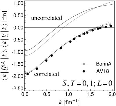
Figure 21: Correlated and uncorrelated Bonn-A and Argonne V18 interaction in momentum representation in the $S,T=0,1$; $L=0$ channel. Symbols denote the corresponding diagonal elements of $V_{\mathit{low-k}}$, taken from [13].

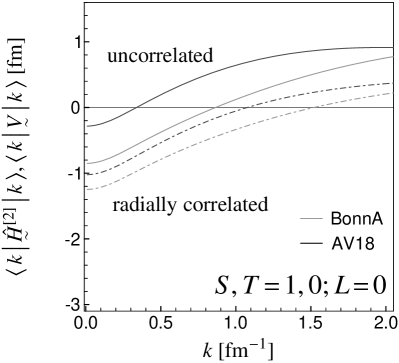
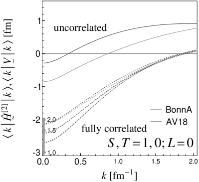
Figure 22: Diagonal matrix elements in momentum space of the correlated (dashed) and uncorrelated (solid) Bonn-A and Argonne V18 interaction in the $S,T=1,0$; $L=0$ channel. Left: only radial correlations are used. Right: radial and tensor correlations are included. The three short-dashed curves show the results with the three tensor correlators ($\alpha$, $\beta$, $\gamma$) of different ranges. The $V_{\mathit{low-k}}$ potential depends in this channel strongly on the cutoff $\Lambda$. The matrix elements for $k=0$ with the cutoffs $\Lambda=1.0,1.5,2.0\>\mathrm{fm}^{-1}$ are indicated.

In Fig. 22 the diagonal matrix elements in the $S,T=1,0$ and $L=0$ channel are shown. Due to the different shapes of the central potentials $v^{c}_{10}(r)$ in this channel (see Fig. 4) the matrix elements of the uncorrelated Bonn-A and Argonne V18 interaction are quite different. The tensor force does not contribute in the uncorrelated case because of $L=0$. The application of the radial correlator makes both interactions more attractive but they still differ significantly. The additional application of tensor correlator which admixes $L=2$ leads for all three tensor correlators ($\alpha$, $\beta$, $\gamma$) not only to strong attraction but also to almost identical correlated interactions.

This shows that two potentials that describe equally well the low energy phase shifts may not only differ in their short range behaviour but also with respect to their relative strength between central and tensor interaction. Nevertheless the unitary correlator maps on the same low momentum effective interaction that reflects only the low momentum properties of nuclear scattering.

For the tensor correlations it is not possible to get a clear separation of scales between short and medium to long range correlations in the many-body state. Therefore in the unitary correlator method the correlation range is not unique. In the language of the $V_{\mathit{low-k}}$ potential ($k$ dependence not published for $S,T=1,0$) this problem is revealed by the fact that the potential cannot be made independent of the cutoff anymore.

6 Many-body calculations

In this section many-body calculations of the ground state properties of the doubly magic nuclei $\@@nuc{4}{He}$, $\@@nuc{16}{O}$ and $\@@nuc{40}{Ca}$ are performed using the Bonn-A and Argonne V18 interactions and their corresponding correlators determined in Sec. 5. Of particular interest is the role of the tensor correlator. The tensor correlator derived according to Eq. (70) from the deuteron or the zero-energy scattering solution is of very long range. It includes due to its naive construction even the non-vanishing $d$-wave outside the range of the interaction. As we want to use the two-body approximation we have to restrict the range of the correlator. To study the influence of the correlation range on the many-body system we will compare the results obtained with the three differently ranged tensor correlators $\alpha$, $\beta$ and $\gamma$. We investigate the question how long ranged the correlator must be to successfully describe the tensor correlations and how short ranged it has to be if we want to restrict ourselves to the two-body approximation.

The many-body calculations are done with the harmonic oscillator shell-model trial states

$$\big{|}\,{\@@nuc{4}{He}}\,\big{>} =\big{|}\,{(1s)^{4}}\,\big{>}$$ (101)

$$\big{|}\,{\@@nuc{16}{O}}\,\big{>} =\big{|}\,{(1s)^{4}(1p)^{12}}\,\big{>}$$ (102)

$$\big{|}\,{\@@nuc{40}{Ca}}\,\big{>} =\big{|}\,{(1s)^{4}(1p)^{12}(2s)^{4}(1d)^{20}}\,\big{>}\;.$$ (103)

The correlated interactions are used in two-body approximation and we can use the correlated operators given in Sec. 4.4.

6.1 The $\@@nuc{4}{He}$ Nucleus

We will discuss the calculations in the $\@@nuc{4}{He}$ nucleus in some detail to illustrate the formalism. The most simple uncorrelated trial state $\big{|}\,{\@@nuc{4}{He}}\,\big{>}$ is the product of a harmonic oscillator ground state wave function with different spins and isospins. The only parameter of the trial state is the oscillator width $a$, that is related to the radius of the $\@@nuc{4}{He}$ nucleus.

This uncorrelated $\@@nuc{4}{He}$ trial state has only $s$-wave components in its relative wave functions and therefore the tensor and spin-orbit forces do not contribute to the expectation value $\big{<}\,{\@@nuc{4}{He}}\,\big{|}\,{{H}_{\mathrm{intr}}}\,\big{|}\,{\@@nuc{4}{He}}\,\big{>}$ of the Hamilton operator. The $d$-wave admixtures in the relative wave functions of the $\@@nuc{4}{He}$ nucleus have to be solely generated by the tensor correlator.

With the Talmi transformation (172) we can calculate the $\@@nuc{4}{He}$ expectation value of the Hamilton operator in two-body approximation

$$\big{<}\,{\@@nuc{4}{He}}\,\big{|}\,{\bigl{[}{C}_{r}^{\dagger}{C}_{\Omega}^{\dagger}{H}_{\mathrm{intr}}{C}_{\Omega}^{\phantom{\dagger}}{C}_{r}^{\phantom{\dagger}}\bigr{]}^{C2}}\,\big{|}\,{\@@nuc{4}{He}}\,\big{>}=\big{<}\,{\@@nuc{4}{He}}\,\big{|}\,{{T}-{T}_{\mathrm{cm}}}\,\big{|}\,{\@@nuc{4}{He}}\,\big{>}\\ \begin{aligned} &+3\big{<}\,{1;(00)0;1}\,\big{|}\,{{c}_{r}^{\dagger}{t}{c}_{r}^{\phantom{\dagger}}-{t}}\,\big{|}\,{1;(00)0;1}\,\big{>}+3\big{<}\,{1;(01)1;0}\,\big{|}\,{{c}_{r}^{\dagger}{c}_{\Omega}^{\dagger}{t}{c}_{\Omega}^{\phantom{\dagger}}{c}_{r}^{\phantom{\dagger}}-{t}}\,\big{|}\,{1;(01)1;0}\,\big{>}\\ &+3\big{<}\,{1;(00)0;1}\,\big{|}\,{{c}_{r}^{\dagger}{v}{c}_{r}^{\phantom{\dagger}}}\,\big{|}\,{1;(00)0;1}\,\big{>}+3\big{<}\,{1;(01)1;0}\,\big{|}\,{{c}_{r}^{\dagger}{c}_{\Omega}^{\dagger}{v}{c}_{\Omega}^{\phantom{\dagger}}{c}_{r}^{\phantom{\dagger}}}\,\big{|}\,{1;(01)1;0}\,\big{>}.\end{aligned}$$ (104)

The expectation value $\big{<}\,{\@@nuc{4}{He}}\,\big{|}\,{{T}-{T}_{\mathrm{cm}}}\,\big{|}\,{\@@nuc{4}{He}}\,\big{>}$ can be calculated analytically, see Eq. (175).

In the $S=0$ channel, where we only have to deal with radial correlations, we get for the two-body matrix element of the correlated kinetic energy

$$\big{<}\,{1;(00)0;1}\,\big{|}\,{{c}_{r}^{\dagger}{t}{c}_{r}^{\phantom{\dagger}}-{t}}\,\big{|}\,{1;(00)0;1}\,\big{>}=\\ -\int\!\mathrm{d}{r}\;\;r\phi_{10}(r)\frac{1}{2\hat{\mu}_{r01}(r)}(r\phi_{10})^{\prime\prime}(r)+\int\!\mathrm{d}{r}\;\;(r\phi_{10}(r))^{2}\ \hat{w}_{01}(r)\;,$$ (105)

see Eq. (52). The reduced mass $\hat{\mu}_{rST}(r)$ and local potential $\hat{w}_{ST}(r)$, defined in Eqs. (53) and (54), respectively, depend on the radial correlation function $R_{+}^{ST}(r)$ of the respective $S,T$ channel. The relative wave function of the two-body states $\big{|}\,{n;(LS)J,T}\,\big{>}$ are harmonic oscillator states with twice the variance of the single-particle states, thus

$$\phi_{10}(r)=\left(\frac{2}{\pi a^{3}}\right)^{\frac{1}{4}}\exp\left\{-\frac{r^{2}}{4a}\right\}$$ (106)

is the radial wave function of the relative motion for $n=1$ and $L=0$.

In the $S=1$ channel also the tensor correlations have to be considered and we get with help of Eqs. (84) and (85)

$$\big{<}\,{1;(01)1;0}\,\big{|}\,{{c}_{r}^{\dagger}{c}_{\Omega}^{\dagger}{t}{c}_{\Omega}^{\phantom{\dagger}}{c}_{r}^{\phantom{\dagger}}-{t}}\,\big{|}\,{1;(01)1;0}\,\big{>}=-\int\!\mathrm{d}{r}\;\;r\phi_{10}(r)\frac{1}{2\hat{\mu}_{r10}(r)}(r\phi_{10})^{\prime\prime}(r)\\ \begin{aligned} &+\int\!\mathrm{d}{r}\;\;(r\phi_{10}(r))^{2}\frac{1}{m}\bigl{[}\theta^{(1)}{}^{\prime}(R_{+}^{10}(r))\bigr{]}^{2}+\int\!\mathrm{d}{r}\;\;(r\phi_{10}(r))^{2}\ \hat{w}_{10}(r)\\ &+\int\!\mathrm{d}{r}\;\;(r\phi_{10}(r))^{2}\sin^{2}\left(\theta^{(1)}(R_{+}^{10}(r))\right)\frac{1}{m(R_{+}^{10}(r))^{2}}\big{<}\,{(21)1}\,\big{|}\,{{\boldsymbol{{l}}}^{2}}\,\big{|}\,{(21)1}\,\big{>}\;.\end{aligned}$$ (107)

In the $S,T=0,1$ channel only the radial part contributes to the matrix element of the potential

$$\big{<}\,{1;(00)0;1}\,\big{|}\,{{c}_{r}^{\dagger}{v}{c}_{r}^{\phantom{\dagger}}}\,\big{|}\,{1;(00)0;1}\,\big{>}=\int\!\mathrm{d}{r}\;\;(r\phi_{10}(r))^{2}\>v^{c}_{01}(R_{+}^{01}(r))\;,$$ (108)

but in the $S,T=1,0$ channel we have to consider also the spin-orbit and tensor force. The expectation value of the central force does not change when including the tensor correlation. The spin-orbit force has only diagonal matrix elements in the $L=2$ states whereas the tensor force has strong off-diagonal contributions between the $L=0$ and $L=2$ states, see Eqs. (86-88):

$$\big{<}\,{1;(01)1;0}\,\big{|}\,{{c}_{r}^{\dagger}{c}_{\Omega}^{\dagger}{v}{c}_{\Omega}^{\phantom{\dagger}}{c}_{r}^{\phantom{\dagger}}}\,\big{|}\,{1;(01)1;0}\,\big{>}=\int\!\mathrm{d}{r}\;\;(r\phi_{10}(r))^{2}v^{c}_{10}(R_{+}^{10}(r))\\ \begin{aligned} &+\int\!\mathrm{d}{r}\;\;(r\phi_{10}(r))^{2}\sin^{2}\left(\theta^{(1)}(R_{+}^{10}(r)\right)\,v^{b}_{10}(R_{+}^{10}(r))\ \big{<}\,{(21)1;0}\,\big{|}\,{{\boldsymbol{{l}}}\!\cdot\!{\boldsymbol{{s}}}}\,\big{|}\,{(21)1;0}\,\big{>}\\ &+2\int\!\mathrm{d}{r}\;\;(r\phi_{10}(r))^{2}\cos\left(\theta^{(1)}(R_{+}^{10}(r)\right)\sin\left(\theta^{(1)}(R_{+}^{10}(r))\right)\,v^{t}_{10}(R_{+}^{10}(r))\\ &\qquad\qquad\times\big{<}\,{(01)1;0}\,\big{|}\,{{s}_{\!12}(\hat{\boldsymbol{{r}}},\hat{\boldsymbol{{r}}})}\,\big{|}\,{(21)1;0}\,\big{>}\\ &+\int\!\mathrm{d}{r}\;\;(r\phi_{10}(r))^{2}\sin^{2}\left(\theta^{(1)}(R_{+}^{10}(r)\right)\,v^{t}_{10}(R_{+}^{10}(r))\ \big{<}\,{(21)1;0}\,\big{|}\,{{s}_{\!12}(\hat{\boldsymbol{{r}}},\hat{\boldsymbol{{r}}})}\,\big{|}\,{(21)1;0}\,\big{>}\;.\end{aligned}$$ (109)

The other components of the interaction have to be treated accordingly.

The correlations also influence the radius of the nucleus. The rms-radius defined as

$$r_{\mathrm{rms}}^{2}=\frac{1}{A}\big{<}\,{\sum_{i=1}^{A}({\boldsymbol{{r}}}_{i}-{\boldsymbol{{R}}}_{\mathrm{cm}})^{2}}\,\big{>}=\frac{1}{A}\big{<}\,{\bigl{(}\sum_{i=1}^{A}{\boldsymbol{{r}}}_{i}^{2}-{\boldsymbol{{R}}}_{\mathrm{cm}}^{2}\bigr{)}}\,\big{>}$$ (110)

is obtained as a sum of the uncorrelated mean square radius and a correction from the radial correlations.

$$\begin{split}r_{\mathrm{rms}}^{2}&=\frac{1}{4}\big{<}\,{\@@nuc{4}{He}}\,\big{|}\,{{C}_{r}^{\dagger}{C}_{\Omega}^{\dagger}\ \bigl{(}\sum_{i=1}^{4}{\boldsymbol{{r}}}_{i}^{2}-{\boldsymbol{{R}}}_{\mathrm{cm}}^{2}\bigr{)}{C}_{\Omega}^{\phantom{\dagger}}{C}_{r}^{\phantom{\dagger}}}\,\big{|}\,{\@@nuc{4}{He}}\,\big{>}\\ &=\frac{1}{4}\big{<}\,{\@@nuc{4}{He}}\,\big{|}\,{\bigl{(}\sum_{i=1}^{4}{\boldsymbol{{r}}}_{i}^{2}-{\boldsymbol{{R}}}_{\mathrm{cm}}^{2}\bigr{)}}\,\big{|}\,{\@@nuc{4}{He}}\,\big{>}+\Delta r_{\mathrm{rms}}^{2}\end{split}$$ (111)

For calculating $\Delta r_{\mathrm{rms}}^{2}$ one uses that the center of mass operator ${\boldsymbol{{R}}}_{\mathrm{cm}}=\frac{1}{A}\sum_{i=1}^{A}{\boldsymbol{{r}}}_{i}$ commutes with ${C}_{r}^{\phantom{\dagger}}$ and ${C}_{\Omega}^{\phantom{\dagger}}$ and $r^{2}_{ij}=({\boldsymbol{{r}}}_{i}-{\boldsymbol{{r}}}_{j})^{2}$ commutes with ${C}_{\Omega}^{\phantom{\dagger}}$. In two-body approximation it is given as

$$\begin{split}\Delta r_{\mathrm{rms}}^{2}&=\frac{3}{4}\big{<}\,{1;(00)0;1}\,\big{|}\,{\frac{1}{2}\left({c}_{r}^{\dagger}{r}^{2}{c}_{r}^{\phantom{\dagger}}-r^{2}\right)}\,\big{|}\,{1;(00)0;1}\,\big{>}\\ &\phantom{=}+\frac{3}{4}\big{<}\,{1;(01)1;0}\,\big{|}\,{\frac{1}{2}\left({c}_{r}^{\dagger}{r}^{2}{c}_{r}^{\phantom{\dagger}}-r^{2}\right)}\,\big{|}\,{1;(01)1;0}\,\big{>}\\ &=\frac{3}{4}\int\!\mathrm{d}{r}\;\;(r\phi_{10}(r))^{2}\biggl{\{}\frac{1}{2}\left(R_{+}^{01}(r)^{2}-r^{2}\right)+\frac{1}{2}\left(R_{+}^{10}(r)^{2}-r^{2}\right)\biggr{\}}\;.\end{split}$$ (112)

The contribution of $\Delta r_{\mathrm{rms}}^{2}$ is however less than one percent.

6.1.1 Results - Argonne V8’

The Argonne V8’ is simpler in its operator structure than the full Argonne V18 interaction and has been used recently as a benchmark potential for many-body calculations of the $\@@nuc{4}{He}$ nucleus [24]. All the quasi-exact many-body methods presented in Ref. [24] agree with each other. We can therefore use their results as a reliable reference for testing our approximation.

Figure 23: Contributions of the Argonne V8’ interaction in $\@@nuc{4}{He}$. For the intrinsic kinetic energy $\big{<}\,{{T}-{T}_{\mathrm{cm}}}\,\big{>}$, the spin-orbit $\big{<}\,{{V}^{b}}\,\big{>}$ and the tensor potential $\big{<}\,{{V}^{t}}\,\big{>}$ three curves for the tensor correlators $\alpha$, $\beta$ and $\gamma$ are shown. The central interaction $\big{<}\,{{V}^{c}}\,\big{>}$ (full line and grey dot) is not influenced by the tensor correlations. $\@@nuc{4}{He}$ optimized correlators are used. Reference values [24] are given by the dots.

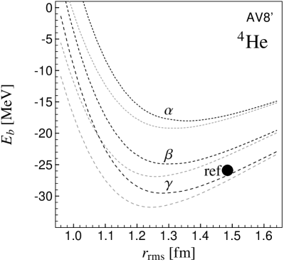
Figure 24: $\@@nuc{4}{He}$ binding energies with the Argonne V8’ interaction (without Coulomb interaction) as a function of the matter radius $r_{\mathrm{rms}}$. Black lines: two-body minimized radial correlators and tensor correlators with restricted range (labeled with $\alpha$, $\beta$, $\gamma$). Gray lines: $\@@nuc{4}{He}$ optimized correlators instead. The result of the reference calculations [24] is included.

In Fig. 23 the contributions of the kinetic energy, the central, spin-orbit and tensor interaction to the total energy are shown as a function of the rms-radius when the oscillator parameter $a$ is varied. The correlation functions are obtained by minimizing the total energy for a given parameter $a$ under the constraints (96) that restrict the range of the tensor correlation with $\alpha$ (dotted line) denoting the shortest one. The expectation value $\big{<}\,{{V}^{c}}\,\big{>}$ (full line and grey point) is not influenced by the tensor correlations as ${V}^{c}$ commutes with ${C}_{\Omega}^{\phantom{\dagger}}$. The spin-orbit contribution $\big{<}\,{{V}^{b}}\,\big{>}$ dependence is rather weak. As expected the variations in the tensor correlator have the largest impact on the expectation value of the tensor interaction $\big{<}\,{{V}^{t}}\,\big{>}$. Without tensor correlations, i.e. ${C}_{\Omega}^{\phantom{\dagger}}=1$, the expectation value $\big{<}\,{{V}^{t}}\,\big{>}$ would vanish completely because we use only the most simple uncorrelated shell-model state of four nucleons in the $s$-shell. The more it is surprising that the correlation function $\vartheta^{\gamma}(r)$ results in almost the exact tensor energy. The correlated kinetic energy increases for shorter ranged correlations because the relative wave functions vary more rapidly and contain higher momenta. The gain in binding in $\big{<}\,{{V}^{t}}\,\big{>}$ is however larger than the loss in $\big{<}\,{{T}-{T}_{\mathrm{cm}}}\,\big{>}$.

In Fig. 24 the sum of all contributions to the binding energy of $\@@nuc{4}{He}$ is shown. The additional black lines denote the results when radial and tensor correlation functions are used that are obtained by minimizing the energy in the two-body system (see Sec. 5). The corresponding energies are almost the same as the ones where the correlation functions are optimized for $\@@nuc{4}{He}$ (gray lines), which indicates that the short range correlations are not very sensitive to the size of the nuclear system but are determined by the nuclear interaction at short distances. We will therefore use in the following only the correlators obtained at $r_{\mathrm{rms}}=1.48\,\mathrm{fm}$.

Fig. 24 also shows that our uncorrelated trial state $\big{|}\,{\@@nuc{4}{He}}\,\big{>}$ is too simple for a precise reproduction of the exact values of binding energy and radius. The delicate balance between large positive and large negative contributions leads to a minimum in the total energy that is at a too small radius. The correlation function $\vartheta^{\beta}(r)$ gives about the correct energy but a radius which is 0.17 fm too small. In order to keep the three- and higher-body contributions small we should use the short-range correlator labelled $\alpha$ and admix $L=2$ states of the relative motion in the trial state explicitly. In that case we would start at the minimum of the dotted black curve at about $r_{\mathrm{rms}}\approx 1.35\ \mathrm{fm}$ and the long range part of the tensor force would admix those states and give the missing binding.

This perception is also supported by Ref. [24] where a probability of 13.9% is quoted to find the nucleus in an $L=2$ eigenstate of the total angular momentum. The uncorrelated $\@@nuc{4}{He}$ trial state has only an $L=0$ component but the tensor correlator induces an $L=2$ admixture. The square of the total orbital angular momentum of the $\@@nuc{4}{He}$ nucleus can be expressed as

$$\big{<}\,{{\boldsymbol{{L}}}^{2}}\,\big{>}=\big{<}\,{\bigl{(}\sum_{i=1}^{A}{\boldsymbol{{r}}}_{i}\times{\boldsymbol{{p}}}_{i}-{\boldsymbol{{L}}}_{\mathrm{cm}}\bigr{)}^{2}}\,\big{>}=\sum_{L=0}L(L+1)P_{L}\;,$$ (113)

where the percentage of an $L$-component is denoted by $P_{L}$. In the two-body approximation this is given by

$$\big{<}\,{\@@nuc{4}{He}}\,\big{|}\,{\left[{C}_{r}^{\dagger}{C}_{\Omega}^{\dagger}{\boldsymbol{{L}}}^{2}{C}_{\Omega}^{\phantom{\dagger}}{C}_{r}^{\phantom{\dagger}}\right]^{C2}}\,\big{|}\,{\@@nuc{4}{He}}\,\big{>}=\\ \begin{split}&=3\big{<}\,{1;(01)1;0}\,\big{|}\,{{c}_{r}^{\dagger}{c}_{\Omega}^{\dagger}{\boldsymbol{{l}}}^{2}{c}_{\Omega}^{\phantom{\dagger}}{c}_{r}^{\phantom{\dagger}}-{\boldsymbol{{l}}}^{2}}\,\big{|}\,{1;(01)1;0}\,\big{>}\\ &=2(2+1)\ 3\int\!\mathrm{d}{r}\;\;(r\phi_{10}(r))^{2}\sin^{2}\left(\theta^{(1)}(R_{+}^{10}(r))\right)\;.\end{split}$$ (114)

There are no contributions from the one-body part of the cluster expansion because all one-body states have $L=0$. From the two-body part the only non-vanishing contribution is in the tensor correlated $S,T=1,0$ channel with its $L=2$ admixture, see Eq. (80). In Table 1 the probalities resulting from the differently ranged correlators are displayed. The correlator $\gamma$ which reproduces the tensor interaction best, see Fig. 23, gives also an $L=2$ contribution that agrees well with the exact one. However, it has also the longest range and hence causes the largest three-body contributions to the correlated interactions which we have neglected. Therefore, we prefer a shorter ranged correlator, for example between $\alpha$ and $\beta$, and an improved trial state that allows for explicit admixture of $d$-waves. In our approximation we do not get any probability for $L=1$, this appears only due to higher particle orders of the correlated Hamiltonian or additional components in the trial state. In any case it is very small as the exact calculations show.

correlator	$P_{L=0}$	$P_{L=1}$	$P_{L=2}$
$\mathit{min}^{\alpha}$	0.959	0.0	0.041
$\mathit{min}^{\beta}$	0.926	0.0	0.074
$\mathit{min}^{\gamma}$	0.881	0.0	0.119
$\mathit{min}^{\alpha}-\@@nuc{4}{He}$	0.956	0.0	0.044
$\mathit{min}^{\beta}-\@@nuc{4}{He}$	0.916	0.0	0.084
$\mathit{min}^{\gamma}-\@@nuc{4}{He}$	0.858	0.0	0.142
Ref. [24]	0.857	0.0037	0.139

Table 1: Probabilities of total orbital angular momentum in $\@@nuc{4}{He}$ for the AV8’ interaction at $r_{\mathrm{rms}}=1.48\;\mathrm{fm}$.

It should be emphasized again that the correlations are absolutely essential for a successful description of the nuclei. As shown in Fig. 3 and discussed in the introduction the existence of bound nuclei can only be explained with the combination of central and tensor correlations.

6.1.2 Results – Bonn-A and Argonne V18

In Fig. 25 we show our results for the $\@@nuc{4}{He}$ nucleus using the Bonn-A and the Argonne V18 interactions. The Argonne V18 nuclear interaction is identical to the Argonne V8’ in the channels relevant in the two-body approximation except for the Coulomb interaction. The energies are plotted against the charge radius that is obtained by folding the many-body charge distribution with the charge distribution of the proton.

For reference we show results of VMC and GFMC calculations [25] with the Argonne V18 interaction. As in the case of the Argonne V8’ interactions we observe that tensor correlator $\beta$ gives the correct energy but at a somewhat smaller radius. One should however also note the large difference in the radii of the VMC and the GFMC calculations. At the reference radius of the GFMC calculation the long range tensor correlator $\gamma$ reproduces the GFMC binding energy. The differences between the GFMC calculation and the experimental binding energy and radius are interpreted as an indication for the necessity of genuine three-body forces.

For the Bonn-A interaction there are no reference calculations but the results are very similar to the Argonne V18 calculations, except that the Bonn-A interaction is more attractive with the shorter tensor correlators $\alpha$ and $\beta$.

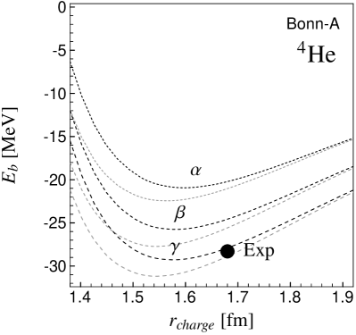
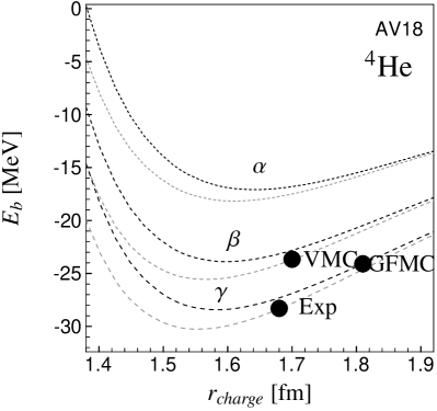
Figure 25: $\@@nuc{4}{He}$ binding energy as function of the rms-charge-radius (including proton size) calculated with the Bonn-A (left hand side) and the Argonne V18 (right hand side) interaction including the Coulomb interaction. Black lines: two-body minimized radial correlators and tensor correlators with restricted range (labeled with $\alpha$, $\beta$, $\gamma$). Gray lines: $\@@nuc{4}{He}$ optimized correlators instead. For the Argonne V18 we the results of VMC and GFMC calculations [25] are included.

6.2 The $\@@nuc{16}{O}$ and the $\@@nuc{40}{Ca}$ nucleus

The doubly magic nuclei are calculated with the harmonic oscillator shell-model trial states given in App. B using the two-body approximation. The evaluation of the two-body matrix elements is done with the correlated interaction in angular momentum eigenstates given in Sec. 4.4 and as it was illustrated for the $\@@nuc{4}{He}$ nucleus.

6.2.1 Results – Argonne V8’

In Fig. 26 our results with the Argonne V8’ interaction are displayed. The FHNC/SOC calculations [8] shown for reference were done with a Hamiltonian consisting of the Argonne V8’ potential together with the Urbana IX three-body force. Therefore we can only compare the expectation values of the Argonne V8’ potential at the radii obtained in the FHNC/SOC calculations. At those radii the $\beta$ and $\gamma$ tensor correlators yield very similar energies.

Figure 26: Binding energy of $\@@nuc{16}{O}$ and $\@@nuc{40}{Ca}$ as function of matter radius $r_{\mathrm{rms}}$ using the Argonne V8’ interaction (Coulomb included). Results for two-body optimized radial correlators and tensor correlators with restricted range (labelled $\alpha$, $\beta$ and $\gamma$). Points denote FHNC/SOC [8] calculations. The radii for the points $a$ and $b$ represent minima of the energy calculated with additional three-body forces. Calculation $a$ used harmonic oscillator states, $b$ and $c$ Woods-Saxon states. Calculation $c$ used a trial state that reproduces the experimental radius.

6.2.2 Results – Bonn-A and Argonne V18

Figure 27: Binding energy of $\@@nuc{16}{O}$ as function of charge radius (including proton size) using the Bonn-A (left) and the Argonne V18 (right) interaction. Results for two-body optimized radial correlators and tensor correlators with restricted range (labelled $\alpha$, $\beta$ and $\gamma$). Result of a Brueckner Hartree Fock (BHF) calculation [26] and a Coupled Cluster (CC) calculation [27] are included.

Figure 28: Binding energy of $\@@nuc{40}{Ca}$ as function of the charge radius (including proton size) using the Bonn-A (left) and the Argonne V18 (right) interaction. Results for two-body optimized radial correlators and tensor correlators with restricted range (labelled $\alpha$, $\beta$ and $\gamma$).

In Fig. 27 and Fig. 28 the results of many-body calculations using the Bonn-A and the Argonne V18 interaction are presented. In case of the Bonn-A interaction the results of a Brueckner Hartree-Fock (BHF) calculation [26] and for the Argonne V18 a Coupled Cluster Calculation [27] are included for reference. It is interesting to note that the Brueckner Hartree-Fock calculation gives the same result as our calculation with a correlator in between $\alpha$ and $\beta$, both in energy and radius. Like in our approximation the BHF method uses an effective two-body Hamiltonian and results in a too small radius. As discussed in the case of the $\@@nuc{4}{He}$ this could be an indication that a single Slater determinant is a too simple trial state and admixtures of particle-hole excitations should describe the long range part of the tensor correlation.

The similarity in the results obtained with the Bonn-A and Argonne V18 interactions as displayed in Figs. 25, 27 and 28 is astonishing. As shown in Fig. 3 the energies obtained with the bare energies are quite different. It seems that the unitary correlators, which are interaction specific, map the two different interactions on the same correlated interaction. This is illustrated further in Sec. 5.6 where the low-momentum behavior of the correlated interaction is discussed.

We can further notice that neither the correlated Argonne V18 nor the correlated Bonn-A interaction can reproduce the experimental binding energies at the experimental radii. It is known from GFMC calculations of light nuclei ($A<8$)[6] that the Argonne V18 interaction does not provide enough binding and additional genuine three-body forces are needed to reproduce the experimental radii and binding energies.

6.3 Momentum distributions

Short range correlations induce high momentum components in the nuclear many-body state that can be seen in the one-body momentum distribution $\hat{n}(\boldsymbol{{k}})$,

$$\hat{n}(\boldsymbol{{k}})=\sum_{\chi,\xi}\big{<}\,{{a}^{\dagger}_{\chi\xi}(\boldsymbol{{k}}){a}^{\phantom{\dagger}}_{\chi\xi}(\boldsymbol{{k}})}\,\big{>}\approx\sum_{\chi,\xi}\big{<}\,{\Phi}\,\big{|}\,{[{C}_{r}^{\dagger}{C}_{\Omega}^{\dagger}{a}^{\dagger}_{\chi\xi}(\boldsymbol{{k}}){a}^{\phantom{\dagger}}_{\chi\xi}(\boldsymbol{{k}}){C}_{\Omega}^{\phantom{\dagger}}{C}_{r}^{\phantom{\dagger}}]^{C2}}\,\big{|}\,{\Phi}\,\big{>}\;,$$ (115)

where ${a}^{\dagger}_{\chi\xi}(\boldsymbol{{k}})$ creates a nucleon with spin $\chi$, isospin $\xi$ and momentum $\boldsymbol{{k}}$. This is another example that, once the unitary correlators ${C}_{\Omega}^{\phantom{\dagger}}$ and ${C}_{r}^{\phantom{\dagger}}$ are determined, not only the Hamiltonian but also any other observable can easily be correlated and although one deals with simple many-body trial states $\big{|}\,{\Phi}\,\big{>}$ that do not contain short range correlations these correlations are not lost like in mean-field models.

Figure 29: Momentum distribution of $\,\@@nuc{4}{He}$ and $\@@nuc{16}{O}$ using the Bonn-A (left) and the Argonne V18 (right) interaction for uncorrelated trial state (thin solid), two-body optimized radial correlators (dashed dotted) and tensor correlators with restricted range ($\alpha$, $\beta$ and $\gamma$). Results of a variational Monte-Carlo (VMC) calculation (grey dots) but using Argonne V14 plus Urbana VII three-nucleon interaction [14] and of a spectral function analysis (grey line) [15] are included.

Figure 29 displays the momentum distributions of $\@@nuc{4}{He}$ and $\@@nuc{16}{O}$ for the Bonn-A and Argonne V18 potential. The thin solid lines denote the uncorrelated shell-model distribution that reproduces the experimental radius. When only the radial correlations are introduced we obtain a contribution at high momenta that is small but reaches out to very high momenta. This is due to the correlation hole at short distances seen in the two-body density in Figs. 1 and 2. The more repulsive AV18 leads to a high momentum tail about twice the one obtained with the Bonn A potential. Introducing also the tensor correlators ${C}_{\Omega}^{\phantom{\dagger}}$ with different ranges $\alpha$, $\beta$, $\gamma$ we obtain a substantial enhancement around $k=2\,\mathrm{fm}^{-1}$. As expected the longer ranged correlator $\gamma$ gives larger momentum distributions than the shorter ranged $\alpha$ and $\beta$, but they all merge for $k>3.5\,\mathrm{fm}^{-1}$. In the $\@@nuc{16}{O}$ AV18 frame we include the results of a variational Monte-Carlo calculation by Pieper et al. [14] (grey dots) which are however for the Argonne V14 interaction supplemented by the Urbana VII three-nucleon interaction. Although the interaction is not the same the comparison shows the importance of the tensor correlator for filling up the momentum distribution around $k=2\,\mathrm{fm}^{-1}$. The distribution corresponding to the spectral function of Benhar et al. [15] which they used successfully to describe inclusive electron-nucleus scattering at large momentum transfer results in the momentum distribution shown as grey full line.

One should however keep in mind that particle-hole excitations in the trial state also contribute in the region of the Fermi surface. As we discussed in Sec. 6 it is better to use a short-ranged correlator $\alpha$ or $\beta$ and describe the long range tensor correlations by the uncorrelated many-body state in order to avoid three- and higher-body terms in the correlated operators.

Appendix A Algebra of operators

In the following sections of the appendix we summarize the properties and the algebra of the operators that appear in processing central and tensor correlations. The symbol $\overset{\scriptstyle{\boldsymbol{{r}}}}{\Rightarrow}$ writes the operator in coordinate representation.

A.1 Radial and orbital momentum operator

The momentum operator ${\boldsymbol{{p}}}$ is decomposed in the radial momentum ${\boldsymbol{{p}}}_{r}$ and the so called orbital momentum ${\boldsymbol{{p}}}_{\Omega}$.

$${\boldsymbol{{p}}}={\boldsymbol{{p}}}_{r}+{\boldsymbol{{p}}}_{\Omega}\;,$$ (116)

The radial momentum is the component in radial direction given by

$${\boldsymbol{{p}}}_{r}=\frac{\boldsymbol{{r}}}{r}p_{r}=\frac{1}{2}\biggl{[}\biggl{(}\boldsymbol{{p}}\cdot\frac{\boldsymbol{{r}}}{r}\biggr{)}\frac{\boldsymbol{{r}}}{r}+\frac{\boldsymbol{{r}}}{r}\biggl{(}\frac{\boldsymbol{{r}}}{r}\cdot\boldsymbol{{p}}\biggr{)}\biggr{]}$$ (117)

and its absolute value is

$${p}_{r}=\frac{1}{2}\biggl{\{}{\boldsymbol{{p}}}\cdot\frac{{\boldsymbol{{r}}}}{{r}}+\frac{{\boldsymbol{{r}}}}{{r}}\cdot\boldsymbol{{p}}\biggr{\}}\;.$$ (118)

Useful coordinate representations of the radial momentum operator are

$$p_{r}\overset{\scriptstyle{\boldsymbol{{r}}}}{\Rightarrow}\frac{1}{i}\biggl{(}\frac{1}{r}+\frac{\partial}{\partial r}\biggr{)}=\frac{1}{i}\frac{1}{r}\frac{\partial}{\partial r}\bigl{(}r\circ\bigr{)}\;,$$ (119)

$$p_{r}^{2}\overset{\scriptstyle{\boldsymbol{{r}}}}{\Rightarrow}-\frac{1}{r}\frac{\partial}{\partial r}\biggl{(}r\frac{1}{r}\frac{\partial}{\partial r}r\circ\biggr{)}=-\frac{1}{r}\frac{\partial^{2}}{\partial r^{2}}\bigl{(}r\circ\bigr{)}\;.$$ (120)

The radial correlator ${c}_{r}^{\phantom{\dagger}}$, which shifts a pair of nucleons only radially in the relative coordinate, is constructed with the generator

$$\begin{split}{g}_{r}&=\frac{1}{2}\Bigr{\{}p_{r}s(r)+s(r)p_{r}\Bigr{\}}=\frac{1}{2}\biggl{\{}\boldsymbol{{p}}\cdot\frac{\boldsymbol{{r}}}{r}s(r)+s(r)\frac{\boldsymbol{{r}}}{r}\cdot\boldsymbol{{p}}\biggr{\}}\\ &\overset{\scriptstyle{\boldsymbol{{r}}}}{\Rightarrow}\frac{i}{2}\biggl{\{}\overleftarrow{\boldsymbol{{\nabla}}}\cdot\frac{\boldsymbol{{r}}}{r}s(r)-s(r)\frac{\boldsymbol{{r}}}{r}\cdot\overrightarrow{\boldsymbol{{\nabla}}}\biggr{\}}=\frac{1}{i}\biggl{\{}\frac{s^{\prime}(r)}{2}+s(r)\frac{\partial}{\partial r}\biggr{\}}\;.\end{split}$$ (121)

Using the above relations the momentum dependent interaction terms can be expressed in different ways

$$\frac{1}{2}\Bigl{(}p_{r}^{2}m(r)+m(r)p_{r}^{2}\Bigr{)} =p_{r}m(r)p_{r}-\frac{1}{2}m^{\prime\prime}(r)-\frac{m^{\prime}(r)}{r}$$ (122)

$$=\left(\boldsymbol{{p}}\cdot\frac{\boldsymbol{{r}}}{r}\right)m(r)\left(\frac{\boldsymbol{{r}}}{r}\cdot\boldsymbol{{p}}\right)-\frac{1}{2}m^{\prime\prime}(r)$$ (123)

$$=\boldsymbol{{p}}\cdot m(r)\boldsymbol{{p}}-m(r)\frac{\boldsymbol{{l}}^{2}}{r^{2}}-\biggl{(}\frac{m^{\prime}(r)}{r}+\frac{1}{2}m^{\prime\prime}(r)\biggr{)}\;.$$ (124)

The orbital momentum ${\boldsymbol{{p}}}_{\Omega}$ is the remaining component that is perpendicular to the distance vector ${\boldsymbol{{r}}}$

$${\boldsymbol{{p}}}_{\Omega}=\frac{1}{2r}\biggl{(}\boldsymbol{{l}}\times\frac{\boldsymbol{{r}}}{r}-\frac{\boldsymbol{{r}}}{r}\times\boldsymbol{{l}}\biggr{)}\;.$$ (42)

It is not to be confused with the orbital angular momentum ${\boldsymbol{{l}}}$. From the definition it is obvious that $\boldsymbol{{p}}_{\Omega}$ commutes with functions which depend only on the relative distance ${r}$ because ${\boldsymbol{{l}}}$ commutes with ${r}$

$$\bigl{[}{\boldsymbol{{p}}_{\Omega}},{f(r)}\bigr{]}_{-}=0\;,$$ (125)

and hence $\boldsymbol{{p}}_{\Omega}$ acts only on the angular degrees of freedom.

The radial momentum operator ${\boldsymbol{{p}}}_{r}$ and the orbital momentum operator ${\boldsymbol{{p}}}_{\Omega}$ do not commute. Using the elementary commutator relations of position and momentum we can verify

$$\bigl{[}{p_{r}},{\boldsymbol{{p}}_{\Omega}}\bigr{]}_{-}=\frac{i}{r}\boldsymbol{{p}}_{\Omega}$$ (126)

and for the scalar product commutator

$$\bigl{[}{\boldsymbol{{p}}_{r}\cdot},{\boldsymbol{{p}}_{\Omega}}\bigr{]}_{-}=\boldsymbol{{p}}_{r}\cdot\boldsymbol{{p}}_{\Omega}-\boldsymbol{{p}}_{\Omega}\cdot\boldsymbol{{p}}_{r}=i\left(p_{r}\frac{1}{r}+\frac{1}{r}p_{r}\right)\overset{\scriptstyle{\boldsymbol{{r}}}}{\Rightarrow}-\frac{1}{r^{2}}+\frac{2}{r}\frac{\partial}{\partial r}\;.$$ (127)

We can further calculate the scalar product commutator with the relative distance operator ${\boldsymbol{{r}}}$

$$\bigl{[}{\boldsymbol{{r}}\cdot},{\boldsymbol{{p}}_{\Omega}}\bigr{]}_{-}=2i$$ (128)

and using

$$\boldsymbol{{p}}^{2}=\boldsymbol{{p}}_{r}^{2}+\boldsymbol{{p}}_{r}\cdot\boldsymbol{{p}}_{\Omega}+\boldsymbol{{p}}_{\Omega}\cdot\boldsymbol{{p}}_{r}+\boldsymbol{{p}}_{\Omega}^{2}\;,$$ (129)

we derive the properties

$$\boldsymbol{{p}}_{r}\cdot\boldsymbol{{p}}_{\Omega}+\boldsymbol{{p}}_{\Omega}\cdot\boldsymbol{{p}}_{r}=-\frac{1}{r^{2}}\;,$$ (130)

$$\boldsymbol{{p}}_{\Omega}^{2}=\frac{1}{r^{2}}\bigl{(}\boldsymbol{{l}}^{2}+1\bigr{)}\;.$$ (131)

A.2 Algebra and matrix elements of tensor operators

We need the algebra of the scalar two-body operators for calculating correlated operators. The determination of the algebra is performed using the irreducible spherical tensor representation of the operators. The conventions of Ref. [28] are used.

A.2.1 Spherical tensor operators

An irreducible spherical tensor operators of rank $k$ is noted as

$${A}^{(k)}_{q}\;.$$ (132)

The transformation from cartesian to spherical tensors of first rank is given by

$${A}^{(1)}_{1}=-\frac{{A}_{x}+i{A}_{y}}{\sqrt{2}}\qquad{A}^{(1)}_{0}={A}_{z}\qquad{A}^{(1)}_{-1}=\frac{{A}_{x}-i{A}_{y}}{\sqrt{2}}\;.$$ (133)

In general two tensor operators of rank $j_{1}$ and $j_{2}$ can be coupled to a tensor operator of rank $j$ using the Clebsch-Gordan coefficients

$$\left\{{{A}^{(j_{1})}}\>{{B}^{(j_{2})}}\right\}^{(j)}_{q}=\sum_{m_{1},m_{2}}\mathrm{C}\Biggl{(}\,\begin{matrix}{j_{1}}&{j_{2}}\\ {m_{1}}&{m_{2}}\end{matrix}\,\Biggr{|}\Biggl{.}\,\begin{matrix}{j}\\ {q}\end{matrix}\,\Biggr{)}\,{A}^{(j_{1})}_{m_{1}}\;{B}^{(j_{2})}_{m_{2}}\;.$$ (134)

A shorthand notation is used for the coupled (and symmetrized) product of vector operators $\boldsymbol{{a}}$ and $\boldsymbol{{b}}$ in coordinate space

$$({{a}}\,{{b}})^{(j)}_{q}=\frac{1}{2}\left(\left\{{{a}^{(1)}}\>{{b}^{(1)}}\right\}^{(j)}_{q}+\left\{{{b}^{(1)}}\>{{a}^{(1)}}\right\}^{(j)}_{q}\right)\;.$$ (135)

The scalar product of spherical tensor operators (acting in different Hilbert spaces) of first rank is given by

$${A}^{(1)}\cdot{T}^{(1)}=-\sqrt{3}\left\{{{A}^{(1)}}\otimes{{T}^{(1)}}\right\}^{(0)}\;,$$ (136)

and the scalar product of spherical tensor operators of second rank by

$${A}^{(2)}\cdot{T}^{(2)}=\sqrt{5}\left\{{{A}^{(2)}}\otimes{{T}^{(2)}}\right\}^{(0)}\;.$$ (137)

Using the spherical tensors we can write for example the spin-orbit operator ${\boldsymbol{{l}}}\!\cdot\!{\boldsymbol{{s}}}$ as

$${\boldsymbol{{l}}}\!\cdot\!{\boldsymbol{{s}}}={l}^{(1)}\cdot{S}^{(1)}=-\sqrt{3}\left\{{{l}^{(1)}}\otimes{{S}^{(1)}}\right\}^{(0)}$$ (138)

and the tensor operator ${s}_{\!12}(\boldsymbol{{a}},\boldsymbol{{b}})$ can be expressed using the spherical tensors as

$$\begin{split}{s}_{\!12}(\boldsymbol{{a}},\boldsymbol{{b}})&=3({\boldsymbol{{\sigma}}}_{1}\cdot{\boldsymbol{{a}}})({\boldsymbol{{\sigma}}}_{2}\cdot{{\boldsymbol{{b}}}})-({\boldsymbol{{\sigma}}}_{1}\cdot{\boldsymbol{{\sigma}}}_{2})({\boldsymbol{{a}}}\cdot{\boldsymbol{{b}}})\\ &=3\left\{{{a}^{(1)}}\>{{b}^{(1)}}\right\}^{(2)}\cdot{S}^{(2)}=3\sqrt{5}\left\{{({a}{b})^{(2)}}\otimes{{S}^{(2)}}\right\}^{(0)}\;,\end{split}$$ (139)

with the operators ${S}^{(1)}$ and ${S}^{(2)}$ in the two-body spin space.

A.2.2 Matrix elements in coordinate space

In coordinate space matrix elements of $\boldsymbol{{r}}$, $\boldsymbol{{p}}_{\Omega}$ and $\boldsymbol{{l}}$ and tensor products of these operators occur. The reduced matrix elements of these elementary operators are given by

$$\big{<}\,{L^{\prime}}\,\big{|}\big{|}\,{{r}^{(1)}}\,\big{|}\big{|}\,{L}\,\big{>}=\bigl{(}\sqrt{L+1}\,\delta_{L^{\prime},L+1}-\sqrt{L}\,\delta_{L^{\prime},L-1}\big{)}r\;,$$ (140)

$$\big{<}\,{L^{\prime}}\,\big{|}\big{|}\,{p_{\Omega}^{(1)}}\,\big{|}\big{|}\,{L}\,\big{>}=\bigl{(}(L+1)^{\frac{3}{2}}\,\delta_{L^{\prime},L+1}+L^{\frac{3}{2}}\,\delta_{L^{\prime},L-1}\bigr{)}\frac{\mathrm{i}}{r}$$ (141)

and

$$\big{<}\,{L^{\prime}}\,\big{|}\big{|}\,{{L}^{(1)}}\,\big{|}\big{|}\,{L}\,\big{>}=\sqrt{L(L+1)(2L+1)}\,\delta_{L^{\prime},L}\;.$$ (142)

The tensor product of two tensor operators can be expressed by the reduced matrixe elements of these operators

$$\big{<}\,{L^{\prime}}\,\big{|}\big{|}\,{\left\{{a^{(k_{1})}}\>{b^{(k_{2})}}\right\}^{(k)}}\,\big{|}\big{|}\,{L}\,\big{>}=\\ (-1)^{L^{\prime}+L-k}\sqrt{2k+1}\sum_{L^{\prime\prime}}\left\{\begin{matrix}{k_{1}}&{k_{2}}&{k}\\ {L}&{L^{\prime}}&{L^{\prime\prime}}\end{matrix}\right\}\big{<}\,{L^{\prime}}\,\big{|}\big{|}\,{a^{(k_{1})}}\,\big{|}\big{|}\,{L^{\prime\prime}}\,\big{>}\big{<}\,{L^{\prime\prime}}\,\big{|}\big{|}\,{b^{(k_{2})}}\,\big{|}\big{|}\,{L}\,\big{>}\;.$$ (143)

With this equation the matrix elements of $s_{\!12}(\boldsymbol{{r}},\boldsymbol{{p}}_{\Omega})$ can be calculated. We get with (140) and (141)

$$\big{<}\,{L}\,\big{|}\big{|}\,{({{r}}\,{{p_{\Omega}}})^{(2)}}\,\big{|}\big{|}\,{L}\,\big{>}=0$$ (144)

and

$$\big{<}\,{L+2}\,\big{|}\big{|}\,{({{r}}\,{{p_{\Omega}}})^{(2)}}\,\big{|}\big{|}\,{L}\,\big{>} =\frac{1}{2}\sqrt{(L+1)(L+2)(2L+3)}\;,$$

$$\big{<}\,{L-2}\,\big{|}\big{|}\,{({{r}}\,{{p_{\Omega}}})^{(2)}}\,\big{|}\big{|}\,{L}\,\big{>} =\frac{1}{2}\sqrt{(L-1)L(2L-1)}\;.$$ (145)

As $s_{\!12}(\boldsymbol{{r}},\boldsymbol{{p}}_{\Omega})$ is a tensor operator of rank 2 all matrix elements with $|L-L^{\prime}|\neq 0,2$ vanish.

A.2.3 Matrix Elements in spin space

In the two-body spin space we have the projectors ${\Pi}_{0}$ onto total spin $0$ and ${\Pi}_{1}$ onto total spin $1$,

$${\Pi}_{0}=\frac{1}{4}(1-{\boldsymbol{{\sigma}}}\otimes{\boldsymbol{{\sigma}}})\;,\qquad{\Pi}_{1}=\frac{1}{4}(3+{\boldsymbol{{\sigma}}}\otimes{\boldsymbol{{\sigma}}})\;,$$ (146)

the total spin operator ${S}^{(1)}$ which is a tensor operator of rank 1

$${S}^{(1)}=\frac{1}{2}\bigl{(}{\sigma}^{(1)}\otimes{1}+{1}\otimes{\sigma}^{(1)}\bigr{)}$$ (147)

and the tensor operator ${S}^{(2)}$ of rank 2

$${S}^{(2)}=\left\{{{S}^{(1)}}\>{{S}^{(1)}}\right\}^{(2)}\;.$$ (148)

The reduced matrix elements of ${S}^{(1)}$ and ${S}^{(2)}$ are given by

$$\big{<}\,{1}\,\big{|}\big{|}\,{{S}^{(1)}}\,\big{|}\big{|}\,{1}\,\big{>}=\sqrt{6}$$ (149)

and

$$\big{<}\,{1}\,\big{|}\big{|}\,{{S}^{(2)}}\,\big{|}\big{|}\,{1}\,\big{>}=2\sqrt{5}\;.$$ (150)

A.2.4 Matrix elements in angular momentum eigenstates

The matrix elements of a scalar product of tensor operators of rank k in coordinate space ${R}^{(k)}$ and spin space ${S}^{(k)}$ is given by

$$\big{<}\,{(L^{\prime}1)JM}\,\big{|}\,{{R}^{(k)}\cdot{S}^{(k)}}\,\big{|}\,{(L1)JM}\,\big{>}=\\ (-1)^{J+L+1}\left\{\begin{matrix}{L^{\prime}}&{L}&{k}\\ {1}&{1}&{J}\end{matrix}\right\}\big{<}\,{L^{\prime}}\,\big{|}\big{|}\,{{R}^{(k)}}\,\big{|}\big{|}\,{L}\,\big{>}\big{<}\,{1}\,\big{|}\big{|}\,{{S}^{(k)}}\,\big{|}\big{|}\,{1}\,\big{>}\;.$$ (151)

With Eqs. (145) and (148) we get the matrix elements of ${s}_{\!12}(\boldsymbol{{r}},\boldsymbol{{p}}_{\Omega})$ in the angular momentum basis

$$\big{<}\,{(J+1,1)JM}\,\big{|}\,{{s}_{\!12}(\boldsymbol{{r}},\boldsymbol{{p}}_{\Omega})}\,\big{|}\,{(J-1,1)JM}\,\big{>} =3\mathrm{i}\sqrt{J(J+1)}\;,$$ (152)

$$\big{<}\,{(J,1)JM}\,\big{|}\,{{s}_{\!12}(\boldsymbol{{r}},\boldsymbol{{p}}_{\Omega})}\,\big{|}\,{(J,1)JM}\,\big{>} =0\;,$$ (153)

$$\big{<}\,{(J-1,1)JM}\,\big{|}\,{{s}_{\!12}(\boldsymbol{{r}},\boldsymbol{{p}}_{\Omega})}\,\big{|}\,{(J+1,1)JM}\,\big{>} =-3\mathrm{i}\sqrt{J(J+1)}$$ (154)

A.2.5 Products of scalar two-body operators

The products, commutators and anti-commutators of scalar two-body operators can be calculated by recoupling the tensor operators with the help of 9j-symbols

$$\left\{{{A}^{(J_{1})}}\otimes{{S}^{(J_{1})}}\right\}^{(0)}\left\{{{B}^{(J_{2})}}\otimes{{T}^{(J_{2})}}\right\}^{(0)}=\\ \sum_{K=0}^{2}(2K+1)\left\{\begin{matrix}{J_{1}}&{J_{1}}&{0}\\ {J_{2}}&{J_{2}}&{0}\\ {K}&{K}&{0}\end{matrix}\right\}\left\{{\left\{{{A}^{(J_{1})}}\>{{B}^{(J_{2})}}\right\}^{(K)}}\otimes{\left\{{{S}^{(J_{1})}}\>{{T}^{(J_{2})}}\right\}^{(K)}}\right\}^{(0)}\;.$$ (155)

Here ${A}$ and ${B}$ are operators in the two-body coordinate space and ${S}$ and ${T}$ are operators in the two-body spin space. Because the two-body spin space is only four dimensional there is no tensor operator with a rank higher than two.

A.3 Cartesian tensor operator relations

Using (155) the following relations for the tensor operators in cartesian representation are obtained

$$({\boldsymbol{{l}}}\!\cdot\!{\boldsymbol{{s}}})^{2}=\frac{2}{3}{\boldsymbol{{l}}}^{2}{\Pi}_{1}-\frac{1}{2}{\boldsymbol{{l}}}\!\cdot\!{\boldsymbol{{s}}}+\frac{1}{6}{s}_{\!12}(\boldsymbol{{l}},\boldsymbol{{l}})\;,$$ (156)

$${s}_{\!12}(\boldsymbol{{r}},\boldsymbol{{p}}_{\Omega})^{2}=6({\boldsymbol{{l}}}^{2}+3){\Pi}_{1}+\frac{45}{2}{\boldsymbol{{l}}}\!\cdot\!{\boldsymbol{{s}}}+\frac{3}{2}{s}_{\!12}(\boldsymbol{{l}},\boldsymbol{{l}})\;.$$ (157)

The commutators needed for the calculation of the correlated interaction are given by

$$\bigl{[}{{s}_{\!12}(\boldsymbol{{r}},\boldsymbol{{p}}_{\Omega})},{{s}_{\!12}(\hat{\boldsymbol{{r}}},\hat{\boldsymbol{{r}}})}\bigr{]}_{-} =-24i{\Pi}_{1}-18i{\boldsymbol{{l}}}\!\cdot\!{\boldsymbol{{s}}}+3i{s}_{\!12}(\hat{\boldsymbol{{r}}},\hat{\boldsymbol{{r}}})$$ (158)

$$\bigl{[}{{s}_{\!12}(\boldsymbol{{r}},\boldsymbol{{p}}_{\Omega})},{{\boldsymbol{{l}}}\!\cdot\!{\boldsymbol{{s}}}}\bigr{]}_{-} =-i{\bar{s}}_{\!12}(\boldsymbol{{p}}_{\Omega},\boldsymbol{{p}}_{\Omega})$$ (159)

$$\bigl{[}{{s}_{\!12}(\boldsymbol{{r}},\boldsymbol{{p}}_{\Omega})},{{\boldsymbol{{l}}}^{2}}\bigr{]}_{-} =2i{\bar{s}}_{\!12}(\boldsymbol{{p}}_{\Omega},\boldsymbol{{p}}_{\Omega})$$ (160)

$$\bigl{[}{{s}_{\!12}(\boldsymbol{{r}},\boldsymbol{{p}}_{\Omega})},{{s}_{\!12}(\boldsymbol{{l}},\boldsymbol{{l}})}\bigr{]}_{-} =7i{\bar{s}}_{\!12}(\boldsymbol{{p}}_{\Omega},\boldsymbol{{p}}_{\Omega})$$ (161)

$$\bigl{[}{{s}_{\!12}(\boldsymbol{{r}},\boldsymbol{{p}}_{\Omega})},{{\bar{s}}_{\!12}(\boldsymbol{{p}}_{\Omega},\boldsymbol{{p}}_{\Omega})}\bigr{]}_{-} =i(96{\boldsymbol{{l}}}^{2}+108){\Pi}_{1}+i(36{\boldsymbol{{l}}}^{2}+153){\boldsymbol{{l}}}\!\cdot\!{\boldsymbol{{s}}}+15i{s}_{\!12}(\boldsymbol{{l}},\boldsymbol{{l}})$$ (162)

$$\bigl{[}{{s}_{\!12}(\boldsymbol{{r}},\boldsymbol{{p}}_{\Omega})},{{\boldsymbol{{l}}}^{2}{\boldsymbol{{l}}}\!\cdot\!{\boldsymbol{{s}}}}\bigr{]}_{-} =-i({\boldsymbol{{l}}}^{2}+3){\bar{s}}_{\!12}(\boldsymbol{{p}}_{\Omega},\boldsymbol{{p}}_{\Omega})$$ (163)

$$\bigl{[}{{s}_{\!12}(\boldsymbol{{r}},\boldsymbol{{p}}_{\Omega})},{{\boldsymbol{{l}}}^{2}{\bar{s}}_{\!12}(\boldsymbol{{p}}_{\Omega},\boldsymbol{{p}}_{\Omega})}\bigr{]}_{-} =i(144{\boldsymbol{{l}}}^{4}+600\boldsymbol{{l}}^{2}+324){\Pi}_{1}$$

$$\quad+i(36{\boldsymbol{{l}}}^{4}+477{\boldsymbol{{l}}}^{2}+477){\boldsymbol{{l}}}\!\cdot\!{\boldsymbol{{s}}}+i(27{\boldsymbol{{l}}}^{2}+51){s}_{\!12}(\boldsymbol{{l}},\boldsymbol{{l}})\;,$$ (164)

where the abbreviation

$${\bar{s}}_{\!12}(\boldsymbol{{p}}_{\Omega},\boldsymbol{{p}}_{\Omega})=2r^{2}{s}_{\!12}(\boldsymbol{{p}}_{\Omega},\boldsymbol{{p}}_{\Omega})+{s}_{\!12}(\boldsymbol{{l}},\boldsymbol{{l}})-\frac{1}{2}{s}_{\!12}(\hat{\boldsymbol{{r}}},\hat{\boldsymbol{{r}}})\;,$$ (165)

is used.

Appendix B Harmonic oscillator shell-model states and Talmi transformation

The single-particle harmonic oscillator states used in the shell model [29]

$$\begin{split}\phi^{a}_{nlm}(\boldsymbol{{r}})&=\frac{R_{nl}(a)(r)}{r}Y^{l}_{m}(\hat{\boldsymbol{{r}}})\\ &=\frac{1}{\Gamma(l+\frac{3}{2})}\frac{\sqrt{2\Gamma(l+n+\frac{1}{2})}}{\sqrt{\Gamma(n)}}\frac{1}{\sqrt{a}^{l+\frac{3}{2}}}e^{-\frac{r^{2}}{2a}}r^{l}F\Bigl{(}1-n,l+\frac{3}{2};\frac{r^{2}}{a}\Bigr{)}Y^{l}_{m}(\hat{\boldsymbol{{r}}})\end{split}$$ (166)

have the unique feature of allowing the separation of center-of-mass and internal motion in a two-body product state. This property can be used in the calculation of interaction matrix elements with the help of the Talmi transformation.

B.1 Talmi coefficients

The Talmi coefficients [29, 30] provide the transformation of a product of two single-particle oscillator wave functions to the product of a function of the center-of-mass motion $\boldsymbol{{R}}=\frac{1}{2}(\boldsymbol{{r}}_{1}+\boldsymbol{{r}}_{2})$ and a function of the relative motion depending on the relative position vector $\boldsymbol{{r}}=\boldsymbol{{r}}_{1}-\boldsymbol{{r}}_{2}$

$$\phi^{a}_{n_{1}l_{1}m_{1}}(\boldsymbol{{r}}_{1})\phi^{a}_{n_{2}l_{2}m_{2}}(\boldsymbol{{r}}_{2})=\sum_{NLMnlm}\left<\begin{matrix}{n_{1}l_{1}m_{1}}\\ {n_{2}l_{2}m_{2}}\end{matrix}\right|\left.\begin{matrix}{NLM}\\ {nlm}\end{matrix}\right>\phi^{a/2}_{NLM}(\boldsymbol{{R}})\,\phi^{2a}_{nlm}(\boldsymbol{{r}})\;.$$ (167)

We calculate the Talmi coefficient by explicitly performing the integrals over the oscillator wave functions.

With the help of the Talmi transformation matrix elements of operators depending only on the relative motion can be calculated as

$$\big{<}\,{n_{1}l_{1}m_{1};n_{2}l_{2}m_{2}}\,\big{|}\,{{v}}\,\big{|}\,{n^{\prime}_{1}l^{\prime}_{1}m^{\prime}_{1};n^{\prime}_{2}l^{\prime}_{2}m^{\prime}_{2}}\,\big{>}=\\ \sum_{\begin{subarray}{c}NLM\\ nlmn^{\prime}l^{\prime}m^{\prime}\end{subarray}}\left<\begin{matrix}{n_{1}l_{1}m_{1}}\\ {n_{2}l_{2}m_{2}}\end{matrix}\right|\left.\begin{matrix}{NLM}\\ {nlm}\end{matrix}\right>\left<\begin{matrix}{n^{\prime}_{1}l^{\prime}_{1}m^{\prime}_{1}}\\ {n^{\prime}_{2}l^{\prime}_{2}m^{\prime}_{2}}\end{matrix}\right|\left.\begin{matrix}{NLM}\\ {n^{\prime}l^{\prime}m^{\prime}}\end{matrix}\right>\big{<}\,{nlm}\,\big{|}\,{{v}}\,\big{|}\,{n^{\prime}l^{\prime}m^{\prime}}\,\big{>}\;,$$ (168)

with the relative wave functions

$$\big{<}\,{\boldsymbol{{r}}}\,\big{|}\,{nlm}\,\big{>}=\phi^{2a}_{nlm}(\boldsymbol{{r}})\;.$$ (169)

Including the spin $\chi$ and isospin $\xi$ degrees of freedom we get for scalar and isoscalar operators the following result

$$\big{<}\,{n_{1}l_{1}m_{1}\chi_{1}\xi_{1};n_{2}l_{2}m_{2}\chi_{2}\xi_{2}}\,\big{|}\,{{v}}\,\big{|}\,{n^{\prime}_{1}l^{\prime}_{1}m^{\prime}_{1}\chi^{\prime}_{1}\xi^{\prime}_{1};n^{\prime}_{2}l^{\prime}_{2}m^{\prime}_{2}\chi^{\prime}_{2}\xi^{\prime}_{2}}\,\big{>}=\\ \begin{aligned} &\sum_{\begin{subarray}{c}nn^{\prime}\\ jmll^{\prime}s\\ tm_{t}\end{subarray}}\sum_{\begin{subarray}{c}m_{l}m^{\prime}_{l}\\ m_{s}m^{\prime}_{s}\end{subarray}}\sum_{NLM}\left<\begin{matrix}{n_{1}l_{1}m_{1}}\\ {n_{2}l_{2}m_{2}}\end{matrix}\right|\left.\begin{matrix}{NLM}\\ {nlm_{l}}\end{matrix}\right>\left<\begin{matrix}{n^{\prime}_{1}l^{\prime}_{1}m^{\prime}_{1}}\\ {n^{\prime}_{2}l^{\prime}_{2}m^{\prime}_{2}}\end{matrix}\right|\left.\begin{matrix}{NLM}\\ {n^{\prime}l^{\prime}m^{\prime}_{l}}\end{matrix}\right>\mathrm{C}\Biggl{(}\,\begin{matrix}{{\textstyle\frac{1}{2}}}&{{\textstyle\frac{1}{2}}}\\ {\xi_{1}}&{\xi_{2}}\end{matrix}\,\Biggr{|}\Biggl{.}\,\begin{matrix}{t}\\ {m_{t}}\end{matrix}\,\Biggr{)}\mathrm{C}\Biggl{(}\,\begin{matrix}{{\textstyle\frac{1}{2}}}&{{\textstyle\frac{1}{2}}}\\ {\xi^{\prime}_{1}}&{\xi^{\prime}_{2}}\end{matrix}\,\Biggr{|}\Biggl{.}\,\begin{matrix}{t}\\ {m_{t}}\end{matrix}\,\Biggr{)}\\ &\times\mathrm{C}\Biggl{(}\,\begin{matrix}{{\textstyle\frac{1}{2}}}&{{\textstyle\frac{1}{2}}}\\ {\chi_{1}}&{\chi_{2}}\end{matrix}\,\Biggr{|}\Biggl{.}\,\begin{matrix}{s}\\ {m_{s}}\end{matrix}\,\Biggr{)}\mathrm{C}\Biggl{(}\,\begin{matrix}{{\textstyle\frac{1}{2}}}&{{\textstyle\frac{1}{2}}}\\ {\chi^{\prime}_{1}}&{\chi^{\prime}_{2}}\end{matrix}\,\Biggr{|}\Biggl{.}\,\begin{matrix}{s}\\ {m^{\prime}_{s}}\end{matrix}\,\Biggr{)}\mathrm{C}\Biggl{(}\,\begin{matrix}{l}&{s}\\ {m_{l}}&{m_{s}}\end{matrix}\,\Biggr{|}\Biggl{.}\,\begin{matrix}{j}\\ {m}\end{matrix}\,\Biggr{)}\mathrm{C}\Biggl{(}\,\begin{matrix}{l^{\prime}}&{s}\\ {m^{\prime}_{l}}&{m^{\prime}_{s}}\end{matrix}\,\Biggr{|}\Biggl{.}\,\begin{matrix}{j}\\ {m}\end{matrix}\,\Biggr{)}\big{<}\,{n(ls)j,t}\,\big{|}\,{{v}}\,\big{|}\,{n^{\prime}(l^{\prime}s)j,t}\,\big{>}\;.\end{aligned}$$ (170)

Using this formula the matrix elements of arbitrary shell-model configurations can be calculated.

B.2 Doubly-magic nuclei

For closed-shell nuclei whose ground states are described in the shell model by completely occupied shells we get the following results.

Given are the expectation values for a two-body operator ${A}$ that is defined in the four spin-isospin channels

$${a}=\sum_{ST}{a}_{ST}\;{\Pi}_{ST}\;.$$ (171)

In the case of $\@@nuc{4}{He}$ all nucleons are in the $1s$ one-particle state. There are only contributions from the even channels in the $\@@nuc{4}{He}$ expectation value (the isospin labels have been omitted in the two-body states $\big{|}\,{n(LS)J}\,\big{>}$ for brevity)

$$\big{<}\,{\@@nuc{4}{He}}\,\big{|}\,{{A}}\,\big{|}\,{\@@nuc{4}{He}}\,\big{>}=3\big{<}\,{1(00)0}\,\big{|}\,{{a}_{01}}\,\big{|}\,{1(00)0}\,\big{>}+3\big{<}\,{1(01)1}\,\big{|}\,{{a}_{10}}\,\big{|}\,{1(01)1}\,\big{>}\;.$$ (172)

In $\@@nuc{16}{O}$ the $1s$ and $1p$ shells are fully occupied. We have contributions from the odd channels and contributions with higher relative angular momentum in the even channels

$$\big{<}\,{\@@nuc{16}{O}}\,\big{|}\,{{A}}\,\big{|}\,{\@@nuc{16}{O}}\,\big{>}=\\ \begin{aligned} &6\big{<}\,{1(10)1}\,\big{|}\,{{a}_{00}}\,\big{|}\,{1(10)1}\,\big{>}\\ &+21\big{<}\,{1(00)0}\,\big{|}\,{{a}_{01}}\,\big{|}\,{1(00)0}\,\big{>}+\frac{3}{2}\big{<}\,{2(00)0}\,\big{|}\,{{a}_{01}}\,\big{|}\,{2(00)2}\,\big{>}+\frac{15}{2}\big{<}\,{1(20)2}\,\big{|}\,{{a}_{01}}\,\big{|}\,{1(20)2}\,\big{>}\\ &+21\big{<}\,{1(01)1}\,\big{|}\,{{a}_{10}}\,\big{|}\,{1(01)1}\,\big{>}+\frac{3}{2}\big{<}\,{2(01)1}\,\big{|}\,{{a}_{10}}\,\big{|}\,{2(01)1}\,\big{>}\\ &+\frac{3}{2}\big{<}\,{1(21)1}\,\big{|}\,{{a}_{10}}\,\big{|}\,{1(21)1}\,\big{>}+\frac{5}{2}\big{<}\,{1(21)2}\,\big{|}\,{{a}_{10}}\,\big{|}\,{1(21)2}\,\big{>}+\frac{7}{2}\big{<}\,{1(21)3}\,\big{|}\,{{a}_{10}}\,\big{|}\,{1(21)3}\,\big{>}\\ &+6\big{<}\,{1(11)0}\,\big{|}\,{{a}_{11}}\,\big{|}\,{1(11)0}\,\big{>}+18\big{<}\,{1(11)1}\,\big{|}\,{{a}_{11}}\,\big{|}\,{1(11)1}\,\big{>}+30\big{<}\,{1(11)2}\,\big{|}\,{{a}_{11}}\,\big{|}\,{1(11)2}\,\big{>}\;.\end{aligned}$$ (173)

In $\@@nuc{40}{Ca}$ the $1s$, $1p$, $2s$ and $1d$ shells are fully fully occupied and we obtain

$$\big{<}\,{\@@nuc{40}{Ca}}\,\big{|}\,{{A}}\,\big{|}\,{\@@nuc{40}{Ca}}\,\big{>}=\\ \begin{aligned} &30\big{<}\,{1(10)1}\,\big{|}\,{{a}_{00}}\,\big{|}\,{1(10)1}\,\big{>}+\frac{9}{2}\big{<}\,{2(10)1}\,\big{|}\,{{a}_{00}}\,\big{|}\,{2(10)1}\,\big{>}+\frac{21}{2}\big{<}\,{1(30)3}\,\big{|}\,{{a}_{00}}\,\big{|}\,{1(30)3}\,\big{>}\\ &+\frac{555}{8}\big{<}\,{1(00)0}\,\big{|}\,{{a}_{01}}\,\big{|}\,{1(00)0}\,\big{>}+\frac{105}{8}\big{<}\,{2(00)0}\,\big{|}\,{{a}_{01}}\,\big{|}\,{2(00)0}\,\big{>}+\frac{9}{8}\big{<}\,{3(00)}\,\big{|}\,{{a}_{01}}\,\big{|}\,{3(00)0}\,\big{>}\\ &+\frac{525}{8}\big{<}\,{1(20)2}\,\big{|}\,{{a}_{01}}\,\big{|}\,{1(20)2}\,\big{>}+\frac{45}{8}\big{<}\,{2(20)2}\,\big{|}\,{{a}_{01}}\,\big{|}\,{2(20)2}\,\big{>}+\frac{81}{8}\big{<}\,{1(40)4}\,\big{|}\,{{a}_{01}}\,\big{|}\,{1(40)4}\,\big{>}\\ &+\frac{555}{8}\big{<}\,{1(01)1}\,\big{|}\,{{a}_{10}}\,\big{|}\,{1(01)1}\,\big{>}+\frac{105}{8}\big{<}\,{2(01)1}\,\big{|}\,{{a}_{10}}\,\big{|}\,{2(01)1}\,\big{>}+\frac{9}{8}\big{<}\,{3(01)1}\,\big{|}\,{{a}_{10}}\,\big{|}\,{3(01)1}\,\big{>}\\ &+\frac{105}{8}\big{<}\,{1(21)1}\,\big{|}\,{{a}_{10}}\,\big{|}\,{1(21)1}\,\big{>}+\frac{175}{8}\big{<}\,{1(21)2}\,\big{|}\,{{a}_{10}}\,\big{|}\,{1(21)2}\,\big{>}+\frac{245}{8}\big{<}\,{1(21)3}\,\big{|}\,{{a}_{10}}\,\big{|}\,{1(21)3}\,\big{>}\\ &+\frac{9}{8}\big{<}\,{2(21)1}\,\big{|}\,{{a}_{10}}\,\big{|}\,{2(21)1}\,\big{>}+\frac{15}{8}\big{<}\,{2(21)2}\,\big{|}\,{{a}_{10}}\,\big{|}\,{2(21)2}\,\big{>}+\frac{21}{8}\big{<}\,{2(21)3}\,\big{|}\,{{a}_{10}}\,\big{|}\,{2(21)3}\,\big{>}\\ &+\frac{21}{8}\big{<}\,{1(41)3}\,\big{|}\,{{a}_{10}}\,\big{|}\,{1(41)3}\,\big{>}+\frac{27}{8}\big{<}\,{1(41)4}\,\big{|}\,{{a}_{10}}\,\big{|}\,{1(41)4}\,\big{>}+\frac{33}{8}\big{<}\,{1(41)5}\,\big{|}\,{{a}_{10}}\,\big{|}\,{1(41)5}\,\big{>}\\ &+30\big{<}\,{1(11)0}\,\big{|}\,{{a}_{11}}\,\big{|}\,{1(11)0}\,\big{>}+90\big{<}\,{1(11)1}\,\big{|}\,{{a}_{11}}\,\big{|}\,{1(11)1}\,\big{>}+150\big{<}\,{1(11)2}\,\big{|}\,{{a}_{11}}\,\big{|}\,{1(11)2}\,\big{>}\\ &+\frac{9}{2}\big{<}\,{2(11)0}\,\big{|}\,{{a}_{11}}\,\big{|}\,{2(11)0}\,\big{>}+\frac{27}{2}\big{<}\,{2(11)1}\,\big{|}\,{{a}_{11}}\,\big{|}\,{2(11)1}\,\big{>}+\frac{45}{2}\big{<}\,{2(11)2}\,\big{|}\,{{a}_{11}}\,\big{|}\,{2(11)2}\,\big{>}\\ &+\frac{49}{2}\big{<}\,{1(31)2}\,\big{|}\,{{a}_{11}}\,\big{|}\,{1(31)2}\,\big{>}+\frac{63}{2}\big{<}\,{1(31)3}\,\big{|}\,{{a}_{11}}\,\big{|}\,{1(31)3}\,\big{>}+\frac{77}{2}\big{<}\,{1(31)4}\,\big{|}\,{{a}_{11}}\,\big{|}\,{1(31)4}\,\big{>}\;.\end{aligned}$$ (174)

B.3 Explicit operator expectation values

For some operators the matrix elements in the harmonic oscillator basis can be calculated analytically.

B.3.1 Intrinsic kinetic energy (uncorrelated)

The expectation value of the uncorrelated intrinsic kinetic energy $\big{<}\,{{T}-{T}_{\mathrm{cm}}}\,\big{>}$ is given by

$$\@@nuc{4}{He}:\>\frac{1}{m}\frac{9}{4a}\qquad\@@nuc{16}{O}:\>\frac{1}{m}\frac{69}{4a}\qquad\@@nuc{40}{Ca}:\>\frac{1}{m}\frac{237}{4a}\;.$$ (175)

B.3.2 Coulomb interaction (uncorrelated)

If we neglect the effect of the central correlations on the expectation values of the Coulomb interaction we obtain

$$\@@nuc{4}{He}:\>2\frac{e^{2}}{\sqrt{2\pi a}}\qquad\@@nuc{16}{O}:\>\frac{83}{2}\frac{e^{2}}{\sqrt{2\pi a}}\qquad\@@nuc{40}{Ca}:\>\frac{7905}{32}\frac{e^{2}}{\sqrt{2\pi a}}\;.$$ (176)

B.3.3 Radius $r_{\mathrm{rms}}$ (uncorrelated)

The uncorrelated $r_{\mathrm{rms}}$ radius of the doubly-magic nuclei (or the one-body contribution of the correlated radius) is given by

$$\@@nuc{4}{He}:\>\frac{3}{2\sqrt{2}}\sqrt{a}\qquad\@@nuc{16}{O}:\>\frac{\sqrt{69}}{4\sqrt{2}}\sqrt{a}\qquad\@@nuc{40}{Ca}:\>\frac{\sqrt{237}}{4\sqrt{5}}\sqrt{a}\;.$$ (177)

Appendix C Correlator parameters

C.1 Correlator parameterizations

The correlation functions $R_{+}(r)$ and $\vartheta(r)$ are used in parameterized form. For short distances $r$ they resemble the ones obtained by mapping the constant trial wave function onto the lowest eigenstate in the two-body system. At larger distances they fall off by either an exponential or a double exponential.

In this work we employ the following parameterizations for the radial correlation functions:

$$R_{+}(r)=r+\alpha^{\prime}\left(\frac{r}{\beta}\right)^{\eta}\exp\biggl{\{}-\exp\biggl{\{}\frac{r}{\beta}\biggr{\}}\biggr{\}}\;,$$ (178)

$$R_{+}(r)=r+\alpha^{\prime}\biggl{(}1-\exp\biggl{\{}-\biggl{(}\frac{r}{\gamma}\biggr{)}^{\eta}\biggr{\}}\biggr{)}\exp\biggl{\{}-\frac{r}{\beta}\biggr{\}}$$ (179)

$$R_{+}(r)=r+\alpha^{\prime}\biggl{(}1-\exp\biggl{\{}-\biggl{(}\frac{r}{\gamma}\biggr{)}^{\eta}\biggr{\}}\biggr{)}\exp\biggl{\{}-\exp\biggl{\{}\frac{r}{\beta}\biggr{\}}\biggr{\}}\;.$$ (180)

For the tensor correlation functions $\vartheta(r)$ the parameterizations

$$\vartheta(r)=\alpha^{\prime}\left(1-\exp\biggl{\{}-\biggl{(}\frac{r}{\gamma}\biggr{)}^{\eta}\biggr{\}}\right)\exp\biggl{\{}-\frac{r}{\beta}\biggr{\}}\;,$$ (181)

$$\vartheta(r)=\alpha^{\prime}\left(1-\exp\biggl{\{}-\biggl{(}\frac{r}{\gamma}\biggr{)}^{\eta}\biggr{\}}\right)\exp\biggl{\{}-\exp\biggl{\{}\frac{r}{\beta}\biggr{\}}\biggr{\}}$$ (182)

are used.

C.2 Bonn-A potential

Radial correlation function $R_{+}(r)$
correlator	ST	type	$\alpha^{\prime}$ [fm]	$\beta$ [fm]	$\gamma$ [fm]	$\eta$
$\mathit{min}$	01	(178)	1.199	0.8082		0.7340
$\mathit{min}$	10	(178)	1.132	0.7788		0.8481
$\mathit{min}$	00	(180)	250232	1.406	1000	2
$\mathit{min}$	11	(178)	0.6581	1.198		0.7981
$\mathit{min}-\@@nuc{4}{He}$	01	(178)	1.344	0.8992		0.6990
$\mathit{min}-\@@nuc{4}{He}$	10	(178)	1.256	0.8526		0.8107

Tensor correlation function $\vartheta(r)$
correlator	ST	type	$\alpha^{\prime}$	$\beta$ [fm]	$\gamma$ [fm]	$\eta$
$\mathit{min}^{\alpha}$	10	(182)	10.2655	1.287	4.994	2
$\mathit{min}^{\beta}$	10	(182)	0.60234	1.834	1.215	2
$\mathit{min}^{\gamma}$	10	(182)	0.35938	2.745	0.9249	2
$\mathit{min}$	11	(181)	-0.024735	1.699	1.197	3
$\mathit{min}^{\alpha}-\@@nuc{4}{He}$	10	(182)	4677.8	1.241	100	2
$\mathit{min}^{\beta}-\@@nuc{4}{He}$	10	(182)	3979.5	1.472	100	2
$\mathit{min}^{\gamma}-\@@nuc{4}{He}$	10	(182)	0.47077	2.551	1.109	2
$\mathit{min}-\@@nuc{4}{He}$	10	(181)	0.08402	7.201	0.7413	2

C.3 Argonne V8’ and Argonne V18 potential

Radial correlation function $R_{+}(r)$
correlator	channel	type	$\alpha^{\prime}$ [fm]	$\beta$ [fm]	$\gamma$ [fm]	$\eta$
$\mathit{min}$	01	(178)	1.379	0.8854		0.3723
$\mathit{min}$	10	(178)	1.296	0.8488		0.4187
$\mathit{min}$	00	(180)	0.76554	1.272	0.4243	1
$\mathit{min}$	11	(180)	0.57947	1.3736	0.1868	1
$\mathit{min}-\@@nuc{4}{He}$	01	(178)	1.380	0.9805		0.3362
$\mathit{min}-\@@nuc{4}{He}$	10	(178)	1.372	0.9072		0.4190

Tensor correlation function $\vartheta(r)$
correlator	channel	type	$\alpha^{\prime}$	$\beta$ [fm]	$\gamma$ [fm]	$\eta$
$\mathit{min}^{\alpha}$	10	(182)	530.38	1.298	1000.0	1
$\mathit{min}^{\beta}$	10	(182)	0.92094	1.717	1.590	1
$\mathit{min}^{\gamma}$	10	(182)	0.383555	2.665	0.4879	1
$\mathit{min}$	11	(181)	-0.023686	1.685	0.8646	1
$\mathit{min}^{\alpha}-\@@nuc{4}{He}$	10	(182)	59.026	1.266	100.0	1
$\mathit{min}^{\beta}-\@@nuc{4}{He}$	10	(182)	54.817	1.554	105.42	1
$\mathit{min}^{\gamma}-\@@nuc{4}{He}$	10	(182)	0.54833	2.446	0.883	1
$\mathit{min}-\@@nuc{4}{He}$	10	(181)	0.10965	4.017	0.3034	1

References

- [1] D. Entem and R. Machleidt, Phys. Lett. B524 (2001) 93, nucl-th/0108057.
- [2] R. Machleidt, Adv. Nucl. Phys. 19 (1989) 189.
- [3] R. Machleidt, Phys. Rev. C63 (2001) 024001.
- [4] R. Wiringa, R. Smith and T. Ainsworth, Phys. Rev. C29 (1984) 1207.
- [5] R. Wiringa, V. Stoks and R. Schiavilla, Phys. Rev. C51 (1995) 38.
- [6] S. Pieper and R. Wiringa, Ann. Rev. Nucl. Part. Sci. 51 (2001) 53, nucl-th/0103005.
- [7] P. Navrátil, J. Vary and B. Barrett, Phys. Rev C62 (2000) 054311.
- [8] A. Fabrocini et al., Phys. Rev. C57 (1998) 1668.
- [9] A. Fabrocini, F.A. de Saavedra and G. Co’, Phys. Rev. C61 (2000) 044302.
- [10] H. Feldmeier and J. Schnack, Rev. Mod. Phys. 72 (2000) 655.
- [11] T. Neff, Short-Ranged Central and Tensor Correlations in Nuclear Many-Body Systems, PhD thesis, TU Darmstadt, 2002.
- [12] H. Feldmeier et al., Nucl. Phys. A632 (1998) 61.
- [13] S. Bogner et al., (2001), nucl-th/0108041.
- [14] S. Pieper, R. Wiringa and V. Pandharipande, Phys. Rev. C46 (1992) 1741.
- [15] O. Benhar et al., Nuc. Phys. A579 (1994) 493.
- [16] S. Pieper et al., Phys. Rev. C64 (2001) 014001.
- [17] S. Weinberg, Phys. Lett. B251 (1990) 288.
- [18] S. Weinberg, Nuc. Phys. B363 (1991) 3.
- [19] B. Pudliner et al., Phys. Rev. C56 (1997) 1720.
- [20] R.B. Wiringa et al., Phys. Rev. C62 (2000) 014001.
- [21] R. Roth, Effektive Wechselwirkungen für Quantenflüssigkeiten und Quantengase: Kernmaterie, flüssiges Helium und ultrakalte atomare Fermigase, PhD thesis, TU Darmstadt, 2000.
- [22] G. Brown, Unified Theory of Nuclear Models and Forces, third ed. (North-Holland, 1971).
- [23] J. Forest et al., Phys. Rev. C54 (1996) 646.
- [24] H. Kamada et al., Phys. Rev. C64 (2001) 044001.
- [25] R. Wiringa, Nucl. Phys. A543 (1992) 199.
- [26] H. Müther and A. Polls, Prog. Part. Nucl. Phys 45 (2000) 243.
- [27] J.H. Heisenberg and B. Mihaila, Phys. Rev. C59 (1999) 1440.
- [28] D.A. Varshalovich, A.N. Moskalev and V.K. Khersonskii, Quantum Theory of Angular Momentum (World Scientific, 1988).
- [29] A. Sitenko and V. Tartakovskii, Lectures on the Theory of the Nucleus (Pergamon Press, 1975).
- [30] J. Irvine, Nuclear Structure Theory, First ed. (Pergamon Press, 1972).