Baryonic masses based on the NJL model

Abstract

We employ the Nambu Jona–Lasinio model to determine the vacuum pressure on the quarks in a baryon and hence their density inside. Then we estimate the baryonic masses by implementing the local density approximation for the mean field quark energies obtained in a uniform and isotropic system. We obtain a fair agreement with the experimental masses.

PACS: 12.39.-x, 12.39.Ba, 12.39.Fe, 14.20.-c, 14.20.Dh

1 Introduction

The Nambu Jona–Lasinio (NJL) model is a phenomenological quark model, which entails chiral symmetry breaking at low density and temperature, and chiral symmetry restoration at high density and temperature. In the chirally broken phase, quarks develop a dynamical mass by their interaction with the vacuum.[1, 2]

This model has been employed in many different contexts, for calculations of meson properties, for hot and dense matter and for the study of diquarks (for reviews about the model and its applications see, for example, [3, 4, 5]). It can successfully reproduce various empirical aspects of QCD such as the non–perturbative vacuum structure, dynamical breaking of chiral symmetry, the $U_{A}(1)$ anomaly and explicit flavour $SU(3)$ breaking in the hadronic spectrum. The strong attractive force between quarks in the $J^{P}=0^{+}$ channel induces an instability in the Fock vacuum of massless quarks, thus generating a dynamical mass $m^{*}$ which is typically of the order of a few hundred MeV, in agreement with the constituent quark masses [6, 7, 8, 9, 10].

This latter feature allows one to consider the constituent quark basis generated by dynamical symmetry breaking as a good starting point for the description of hadrons, including baryons. However, beyond the conventional constituent quark model, the NJL model takes into account the collective nature of the vacuum and the Nambu-Goldstone bosons. The remaining non–perturbative effects such as the long–range confinement force can be treated as a relatively weak perturbation for low-energy phenomena. A similar picture has been first applied to baryons in Ref. [12].

In this work, we first connect the NJL model to the evaluation of the typical dimensions of a baryon (in particular the nucleon radius). Then, in the spirit of the constituent quark model, we employ this result to calculate the octet baryon masses.

In Section 2 we recall the main results of the NJL model, such as the chiral condensate for quarks, the expression for the dynamical masses, the energy and pressure of a uniform and isotropic quark system. As it is known, the dynamical masses in the vacuum are quite large compared to the current quark masses (for the quarks $u$ and $d$ one goes from a current quark mass of 5 MeV to an effective mass larger than 300 MeV), but when the density increases the dynamical masses decrease and hence the degree of chiral symmetry breaking, caused by the large effective masses, becomes less severe. A complete chiral restoration can only be achieved when the bare masses $m_{i}$ vanish, but even very small values of $m_{i}$ are enough to prevent it.

We want to apply these considerations to the problem of the stability of the nucleon. First we note that outside the nucleon there is a vacuum pressure ($P_{vac}$) caused by the negative energy of the Dirac sea, but inside the nucleon the pressure due to the Dirac sea ($P_{N,vac}$) is much lower since it is a high density region and the dynamical masses become small. As a consequence one has an effective pressure acting on the nucleon, due to the difference between the energy densities.

The situation is similar to the one encountered in the MIT bag model [13, 14, 15, 16], but here the bag pressure is by itself a model parameter, while in the NJL model the pressures ($P_{vac}$, $P_{N,vac}$) are deduced after tuning the other parameters to reproduce, e.g., the experimental mesonic masses. For a generic attempt to derive the bag pressure see Ref. [17].

The residual effective pressure is equilibrated by the pressure generated by the three quarks inside the nucleon. Obviously one can not consider them as a uniform and isotropic quark system, neither express their pressure with the formulas developed in Section 2. For this purpose, in Section 3 we will assume heuristic wave functions for the quarks confined in the nucleon. Under this assumption we can calculate the quark pressure and, by imposing that it equals the effective vacuum pressure, we can derive the radius of the nucleon, to be compared with the experimental value.

In Section 4 we develop the calculation for the masses of the baryonic octet, utilizing the results of Section 3 and taking into account the dynamical quark masses. The latter are derived by implementing the local density approximation on a uniform gas of quarks to obtain the dependence of the masses upon the distance from the center of the baryon, according to the spatial quark density found in the previous Section. The masses increase with the distance, since the density decreases and vanishes outside the baryon. An analogous procedure is utilized for the kinetic energy contribution to the baryonic mass.

We do not attempt, here, an approach based on the relativistic Faddeev model, quite often implemented from a NJL-type Lagrangian and applied both to the nucleon [18, 19, 20] and to the baryons’ octet and decuplet [21]. The merit of the Faddeev approach is to offer an evaluation of the quark wave function which is consistent with the model Lagrangian employed. Mesonic properties and the masses of the nucleon and $\Delta$ resonance are well reproduced. Yet, the constituent quark masses are kept constant for a given parameter set.

The central and key point of the present work, instead, is to take into account the variation of the constituent masses with the density of quarks inside the hadron: independently of the details of the wave functions employed here, this appears to be crucial in order to get a realistic determination of the baryonic masses. Some warning should apply to the use of the NJL at finite densities (as it has been extensively discussed in ref. [3]), where it can lead to unphysical results, like having, e.g., vanishing or even negative effective mass of the quark. We shall shortly discuss this point in connection with the present calculation.

Finally we also calculate the masses of two baryons from the spin ${3}/{2}$ decuplet, and find that the present calculation provides for them a reasonable estimate, which can be slightly improved by the effect of the spin interaction. We summarize and discuss our results in Section 5.

2 Short review of the NJL model

Many versions of the NJL Lagrangian have been used in the past, particularly in the last ten years; we consider a three flavour NJL Lagrangian of the form [3, 4, 5, 22]:

$${{\mathcal{L}}}_{NJL}={{\mathcal{L}}}_{0}+{{\mathcal{L}}}_{m}+{{\mathcal{L}}}_{(4)}+{{\mathcal{L}}}_{(6)}$$ (1)

where:

$${\mathcal{L}}_{0} = i\,\bar{q}\,\gamma^{\mu}\,\partial_{\mu}q\,,$$ (2)

$${\mathcal{L}}_{m} = -\,\bar{q}\,{\bf\hat{m}}\,q\,,$$ (3)

$${\mathcal{L}}_{(4)} = \frac{G}{2}\sum\limits_{k=0}^{8}\,\left[\left(\bar{q}_{i}(\lambda_{k})_{ij}q_{j}\right)^{2}+\left(i\bar{q}_{i}\gamma_{5}(\lambda_{k})_{ij}q_{j}\right)^{2}\right]\,,$$ (4)

$${\mathcal{L}}_{(6)} = -K\left[\det_{i,j}\left(\bar{q}_{i}(1+\gamma_{5})q_{j}\right)+\det_{i,j}\left(\bar{q}_{i}(1-\gamma_{5})q_{j}\right)\right]\,.$$ (5)

In the above $q\equiv\left({{\begin{array}[]{c}u\\ d\\ s\end{array}}}\right)$ is the quark field, ${\bf\hat{m}}\equiv\left({{\begin{array}[]{ccc}m_{u}&0&0\\ 0&m_{d}&0\\ 0&0&m_{s}\end{array}}}\right)$ is the mass matrix, $\lambda_{1}\ldots\lambda_{8}$ are the Gell–Mann flavour matrices, and $\lambda_{0}\equiv\sqrt{\frac{2}{3}}{\mathbf{1}}$.

${\mathcal{L}}_{(4)}$ generates four–leg interaction vertexes, while ${\mathcal{L}}_{(6)}$ gives rise to six–leg interaction vertexes; $G$ and $K$ are two parameters of the model, with the dimensions of $[L^{2}]$ and $[L^{5}]$, respectively. In the limit of $m_{i}=0$, the symmetries of the model Lagrangian are the following ones:

$$U_{V}(1)\times SU_{V}(3)\times SU_{A}(3)\times SU_{c}(3)$$ (6)

where, of course, $SU_{c}(3)$ is global and not local; $U_{A}(1)$ is broken by the existence of the axial anomaly. For an extended analysis of this NJL Lagrangian, see for example Ref. [2].

Within the mean field approximation it is possible to evaluate the dynamical quark masses, which are generated by the quark–vacuum interaction; we consider homogeneous, isotropic quark matter, with Fermi momenta $p_{F}^{u},p_{F}^{d}$ and $p_{F}^{s}$ for the flavours $u,d$ and $s$, respectively. The result of the calculation is [16] ($i,j,k=u,d,s$):

$$m_{i}^{*}=m_{i}-2G\langle\bar{q}_{i}q_{i}\rangle+2K\langle\bar{q}_{j}q_{j}\rangle\langle\bar{q}_{k}q_{k}\rangle\qquad\quad(i\neq j\neq k)$$ (7)

where

$$\langle\bar{q}_{i}q_{i}\rangle=-\frac{3}{\pi^{2}}\int\limits_{p_{F}^{i}}^{\Lambda}\mathrm{d}p\frac{m_{i}^{*}p^{2}}{\sqrt{p^{2}+(m_{i}^{*})^{2}}}$$ (8)

is the chiral condensate for the $i$-flavour. We introduce a three–dimensional regularization with a cut–off $\Lambda$ since the integral is obviously divergent. It is important to note that as the Fermi momenta increase, the chiral condensate and the dynamical masses decrease. In the vacuum the dynamical masses reach their highest values.

For our purposes it is very important to consider the energy density of the system, which is given by the following formula [16]:

$$\varepsilon=-\sum\limits_{i=u,d,s}\frac{3}{\pi^{2}}\int\limits_{p_{F}^{i}}^{\Lambda}\mathrm{d}pp^{2}\sqrt{p^{2}+(m_{i}^{*})^{2}}+\left[\sum\limits_{i=u,d,s}\,G\langle\bar{q}_{i}q_{i}\rangle^{2}\right]-4K\langle\bar{u}u\rangle\langle\bar{d}d\rangle\langle\bar{s}s\rangle.$$ (9)

The pressure of the system can then be derived to be:

$$P=-\varepsilon+\rho_{i}\mu_{i}$$ (10)

where:

$$\rho_{i}=\frac{\left(p_{F}^{i}\right)^{3}}{\pi^{2}}$$ (11)

is the quark density of flavour $i$ and $\mu_{i}=\sqrt{\left(p_{F}^{i}\right)^{2}+(m_{i}^{*})^{2}}$ the corresponding chemical potential. The pressure of vacuum is then, using formula (9):

$$P_{vac}=-\varepsilon_{vac}=-\varepsilon(p^{i}_{F}=0),$$ (12)

which is positive for the customary choices of the parameters $G$ and $K$.

In the following Sections we will consider two sets of parameters, which have been employed in Refs. [22] (set 1) and [5] (set 2); in both cases the current masses for the $u$ and $d$ quarks are fixed on the basis of isospin symmetry and of limits on the average $\bar{m}=(m_{u}+m_{d})/2$ at 1 GeV scale, while the remaining four parameters are fitted to reproduce the masses of $\pi$, $K$ and $\eta^{\prime}$ mesons, together with the pion–decay constant $f_{\pi}$:

set 1	set 2
$m\equiv m_{u}=m_{d}=5.5$ MeV	$m\equiv m_{u}=m_{d}=5.5$ MeV
$m_{s}=140.7$ MeV	$m_{s}=135.7$ MeV
$\Lambda=602.3$ MeV	$\Lambda=631.4$ MeV
$G\Lambda^{2}=3.67$	$G\Lambda^{2}=3.67$
$K\Lambda^{5}=12.36$	$K\Lambda^{5}=9.29$

With the above values, the effective quark masses in the vacuum and the chiral condensates turn out to be:

	set 1(MeV)	set 2(MeV)
$m^{*}_{u}=m^{*}_{d}$	367.7	335.5
$m^{*}_{s}$	549.5	527.6
$|\langle{\bar{q}}q\rangle_{u}|^{1/3}=|\langle{\bar{q}}q\rangle_{d}|^{1/3}$	241.9	246.7
$|\langle{\bar{q}}q\rangle_{s}|^{1/3}$	257.7	266.7

3 Nucleon radius

We will heuristically assume that a quark confined in a nucleon has a Gaussian wave function; the reasons for this assumption are essentially three: this wave function reproduces the confinement of a particle in a spatial region, it can be treated analytically, and it is also the ground state wave function of an harmonic oscillator. Hence, with the correct normalization, the spatial wave function of the three valence quarks in a nucleon is written as:

$$\Psi_{q}\left(r\right)=\left(\frac{2}{\pi}\right)^{\frac{3}{4}}\frac{1}{b^{\frac{3}{2}}}e^{-\frac{r^{2}}{b^{2}}}$$ (13)

where $b$ is a parameter with the dimension of a length. The total baryonic density is then:

$$\rho_{B}(r)=3\left(\frac{1}{3}\right)\left|\psi_{q}(r)\right|^{2}=\left|\psi_{q}(r)\right|^{2},$$ (14)

which coincides with the probability density for one quark. To fix the parameter $b$ we establish a connection with the properties derived in the NJL model.

First we calculate the following average quantities (average squared radius and average volume) from $\Psi_{q}\left(r\right)$:

$$\langle r^{2}\rangle=\frac{3}{4}b^{2};\hskip 28.45274pt\langle V\rangle=\frac{4}{3}\pi\langle r^{2}\rangle^{3/2}=\frac{\pi\sqrt{3}}{2}b^{3}.$$ (15)

Then, by considering the Fourier transform of $\Psi_{q}\left(r\right)$,

$$A(k)=\frac{b^{3/2}}{(2\pi)^{3/4}}e^{-\frac{1}{4}k^{2}b^{2}}$$ (16)

we can calculate the average kinetic energy of the quark as follows:

$$\langle E_{q}\rangle=4\pi\int\limits_{0}^{\infty}\mathrm{d}kk^{2}\sqrt{(m^{*}_{q})^{2}+k^{2}}\left|A(k)\right|^{2}$$ (17)

where $m^{*}_{q}$ is the dynamical quark mass.

As we have already noticed in the previous Section, the dynamical mass of a quark in a high density region is small, and this is precisely the situation of the quark inside a baryon; therefore, we can eventually neglect $m^{*}_{q}$ in the previous formula, and explicitly obtain, for the average energy of the quark, the analytic expression:

$$\langle E_{q}\rangle\simeq 4\pi\int\limits_{0}^{\infty}\mathrm{d}k\left|A(k)\right|^{2}k^{3}=\frac{4}{\sqrt{2\pi}}\frac{1}{b}=\frac{\gamma}{\langle V\rangle^{1/3}}$$ (18)

where use has been made of relation (15) to express $\langle E_{q}\rangle$ in terms of the average volume and $\gamma=(4/\sqrt{2\pi})\left(\pi\sqrt{3}/2\right)^{1/3}$. In this approximation the total energy density of a nucleon turns then out to be:

$$\langle E_{T}\rangle=3\langle E_{q}\rangle,$$ (19)

from which we can calculate the pressure of the three–quark system as follows:

$$P=-\left(\frac{\partial\langle E_{T}\rangle}{\partial\langle V\rangle}\right)_{N_{q}}=\frac{\gamma}{\langle V\rangle^{4/3}}.$$ (20)

$N_{q}$ being the total (fixed) number of quarks. This quantity obviously depends on the parameter $b$.

In order to set a connection with the NJL model, we shall now evaluate the effective vacuum pressure acting on the nucleon. In the NJL model the energy density can be expressed in the following way:

$$\varepsilon = \varepsilon_{u,d}+\varepsilon_{s}$$ (21)

$$\varepsilon_{u,d} = -\sum\limits_{i=u,d}\frac{3}{\pi^{2}}\int\limits_{p_{F}^{i}}^{\Lambda}\mathrm{d}p\,p^{2}\sqrt{p^{2}+(m_{i}^{*})^{2}}+\sum\limits_{i=u,d}G\langle\bar{q}_{i}q_{i}\rangle^{2}-2K\langle\bar{u}u\rangle\langle\bar{d}d\rangle\langle\bar{s}s\rangle$$

$$\varepsilon_{s} = -\frac{3}{\pi^{2}}\int\limits_{0}^{\Lambda}\mathrm{d}p\,p^{2}\sqrt{p^{2}+(m_{s}^{*})^{2}}+G\langle\bar{s}s\rangle^{2}-\langle\bar{s}s\rangle\left(m_{s}^{*}-m_{s}+2G\langle\bar{s}s\rangle\right)$$

where we have set $p_{F}^{s}$=0, since in the nucleon no strange valence quarks are present. It is possible to show [23] that in this case $\langle\bar{s}s\rangle$ is almost constant with varying $u$ and $d$ densities. In turn, this implies:

$$\frac{\mathrm{d}\varepsilon_{s}}{\mathrm{d}m_{s}^{*}}=\langle\bar{s}s\rangle-\langle\bar{s}s\rangle=0.$$ (22)

By considering that $m^{*}_{s}$ depends on $\rho_{u}$ and $\rho_{d}$ [see eqs. (7), (8)], it follows that:

$$\frac{\partial\varepsilon_{s}}{\partial\rho_{u}}=\frac{\partial\varepsilon_{s}}{\partial\rho_{d}}=0.$$ (23)

For this reason $\varepsilon_{s}$ does not contribute to the pressure acting on the nucleon (it has the same value inside and outside) and in the following we will consider only the $\varepsilon_{u,d}$ contributions.

In the vacuum, with $\rho_{u}=\rho_{d}=0$ (and $p_{F}^{u}=p_{F}^{d}=0$), the $u,d$ contribution to the pressure is then:

$$P_{vac}=-\varepsilon_{u,d(vac)}$$ (24)

which, for the above mentioned two different sets of parameters, turns out to be:

$$\begin{array}[]{l}P_{vac}=2.091\times 10^{10}\,\,({\mathrm{MeV}})^{4}\hskip 56.9055pt{\mbox{(set 1)}}\\ P_{vac}=2.493\times 10^{10}\,\,({\mathrm{MeV}})^{4}\hskip 56.9055pt{\mbox{(set 2)}}\end{array}$$ (25)

Inside the nucleon the vacuum pressure is uniquely related to the Dirac sea energy density; indeed, since in the nucleon interior $u$ and $d$ quark densities are high, we can neglect, as before, their chiral condensate and their masses. Hence we have the following expression for the internal pressure:

$$P_{N,vac}=2\frac{3}{\pi^{2}}\int\limits_{0}^{\Lambda}\mathrm{d}p\,p^{3}=\frac{3}{2\pi^{2}}\Lambda^{4}$$ (26)

with the following numerical values:

$$\begin{array}[]{l}P_{N,vac}=2.00\times 10^{10}\,\,({\mathrm{MeV}})^{4}\hskip 56.9055pt{\mbox{(set 1)}}\\ P_{N,vac}=2.42\times 10^{10}\,\,({\mathrm{MeV}})^{4}\hskip 56.9055pt{\mbox{(set 2)}}.\end{array}$$ (27)

Finally the effective vacuum pressure acting on the nucleon is:

$$P_{eff}=P_{vac}-P_{N,vac}$$ (28)

for which we get:

$$\begin{array}[]{l}P_{eff}=9.13\times 10^{8}\,\,({\mathrm{MeV}})^{4}\hskip 56.9055pt{\mbox{(set 1)}}\\ P_{eff}=7.71\times 10^{8}\,\,({\mathrm{MeV}})^{4}\hskip 56.9055pt{\mbox{(set 2)}}.\end{array}$$ (29)

These values can be compared to the ones of the $B$ parameter in the MIT bag model: the authors of Ref. [24] employed a value $B=4.42\times 10^{8}$ MeV⁴ for reproducing masses and other parameters of light hadrons, while the value $B=7.68\times 10^{8}$ MeV⁴ (very close to our net pressure with parameter set 2) was more appropriate for the hadronic structure functions [25].

In order to have equilibrium, the effective vacuum pressure and the three quark pressure (20) must be equal; by imposing this condition we can then fix the parameter $b$ in terms of the NJL model parameters. We obtain the following values:

$$b = 0.993\,\,{\mathrm{fm}}\hskip 28.45274pt{\mathrm{(set1)}}$$

$$b = 1.036\,\,{\mathrm{fm}}\hskip 28.45274pt{\mathrm{(set2)}}.$$

We can calculate $\langle r^{2}\rangle$ and hence the radius of the nucleon, $R=\sqrt{\langle r^{2}\rangle}$, which turns out to be, for the two parameter sets:

$$\sqrt{\langle r^{2}\rangle} = 0.860~{}~{}\mathrm{fm~{}~{}~{}~{}~{}~{}~{}~{}~{}set}1$$

$$\sqrt{\langle r^{2}\rangle} = 0.897~{}~{}\mathrm{fm~{}~{}~{}~{}~{}~{}~{}~{}~{}set}2$$

in fair agreement with the experimental determination, $\sqrt{\langle r^{2}\rangle_{exp}}$=0.81 fm.

In spite of the simplicity of our approach, this result points to an interesting interpretation, since both the Dirac sea and the vacuum pressure seem to play an important role in the nucleon stability.

In the next section we will use this model for the calculation of the baryon octet masses. The above determination of the value of $b$, in particular the approximation of neglecting the quark masses inside the nucleon, employed in eqs. (18) and (26), will be discussed: indeed it poses a delicate problem of self–consistency, as it will be clarified below.

4 Octet baryon masses

In order to evaluate the baryon masses we sum the energies of the constituent quarks: for this purpose we recall that in the NJL model the effective mass, at fixed density, is given by eqs. (7), (8). We shall implement these expressions by taking into account the quark density inside the baryon, according to the Ansatz (13) for the quark wave function.

The density of $N_{i}$ quarks of flavour $i$ is then:

$$\rho_{i}(r)=N_{i}\left|\psi_{q}^{i}(r)\right|^{2},$$ (30)

with the condition: $N_{u}+N_{d}+N_{s}=3\,$. We can obtain the behaviour of the dynamical mass $m_{i}^{*}(r)$ as a function of the distance $r$ from the center of the baryon by using the so–called Local Density Approximation (LDA). It amounts to define a local Fermi momentum $p_{F}^{i}(r)=[\pi^{2}\rho_{i}(r)]^{{1}/{3}}$ for each flavour of quarks and then insert it into the self–consistent definition of the dynamical mass, which thus becomes $(i\neq j\neq k)$:

$$m_{i}^{*}(r) =m_{i}+\frac{6G}{\pi^{2}}\int\limits_{p_{F}^{i}(r)}^{\Lambda}\mathrm{d}p\frac{m_{i}^{*}(r)p^{2}}{\sqrt{p^{2}+(m_{i}^{*}(r))^{2}}}+$$

$$+2K\left(\frac{3}{\pi^{2}}\right)^{2}\left[\,\int\limits_{p_{F}^{j}(r)}^{\Lambda}\mathrm{d}p\frac{m_{j}^{*}(r)p^{2}}{\sqrt{p^{2}+(m_{j}^{*}(r))^{2}}}\right]\left[\,\int\limits_{p_{F}^{k}(r)}^{\Lambda}\mathrm{d}p\frac{m_{k}^{*}(r)p^{2}}{\sqrt{p^{2}+(m_{k}^{*}(r))^{2}}}\right];$$

the $r$ dependence of $m_{i}^{*}$ is governed by the lower limits of integration and by the self-consistency requirement entailed by eq. (4) itself.

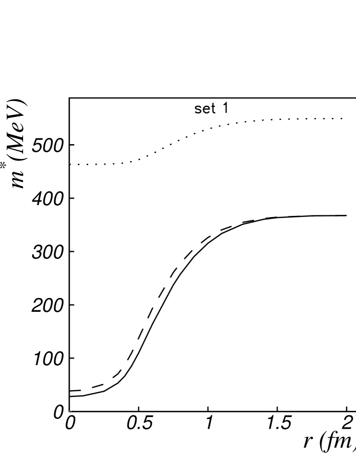
Figure 1: Quark masses as a function of $r$ in the nucleon case for the two different sets of parameters. In both panels, solid lines represent $m_{u}$, dashed lines $m_{d}$ and dotted lines $m_{s}$.

As an example, we show in Fig. 1 the masses of the $u$, $d$ and $s$ quarks in the proton ($N_{u}=2$, $N_{d}=1$, and $N_{s}=0$) as a function of $r$, using the $b$ values obtained in the previous section. One can see that the light quark masses are small for $r\sim 0$, which roughly justifies the approximations of the previous Section. The $s$ quark mass is affected by the quark density in the nucleon only by the six–quark coupling term in the Lagrangian, hence it shows a rather mild variation from the interior to the exterior of the nucleon. On the contrary, the $u$ and $d$ masses are much smaller inside the baryon than outside it.

The density dependence of the effective quark masses, which here and in the following turns out to be one of the most relevant features, deserves some words of criticism. Indeed in the NJL model, the interplay between chemical potential (which defines the Fermi energy and contains the effective mass) and baryon density crucially depends not only on the order of approximation made in solving, for example, the gap equation, but also on the specific values of the model parameters employed. This point has been widely and clearly discussed in the review of Klevansky [3], where the qualitatively different outcomes (e.g. for the quark effective mass as a function of the chemical potential) are elucidated. In particular it is shown that: i) the order of the phase transition which occurs as the density increases depends upon the inclusion of exchange effects in the mean field approximation and ii) the properties of the system with increasing density dramatically depend upon the chosen set of parameters. Of special relevance is the value of the cutoff $\Lambda$ as compared with the chemical potential, since with increasing density a too small cutoff could lead to unphysical negative effective masses. These problems do not specifically affect the results of the present work, but were carefully considered and checked at any stage of the calculation.

To calculate baryonic masses we still need the “local” kinetic energy for the quark; in order to avoid an additional integration over the Fermi sphere for each quark species, we employ the average momentum in the local Fermi sphere, namely $(3/5){p_{F}^{i}}^{2}$. Hence the total baryonic mass reads:

$$M=\sum_{i=u,d,s}\int\limits_{0}^{\infty}\mathrm{d}r~{}4\pi r^{2}\rho_{i}\left(r\right)\sqrt{\frac{3}{5}p_{F}^{i}\left(r\right)^{2}+(m_{i}^{*}\left(r\right))^{2}}.$$ (32)

Baryon	N	$\Lambda$	$\Sigma^{+}$	$\Delta^{++}$	$\Xi^{0}$	$\Omega^{-}$
$m_{exp}$ (MeV)	938.27	1115.68	1189.37	1232	1314.9	1672.45
$m_{set\,1}$ (MeV)	981.22	1150.59	1199.20	1072.28	1349.78	1536.84
$m_{set\,2}$ (MeV)	935.15	1119.71	1159.12	1013.36	1325.96	1517.38

Table I. Experimental masses and theoretical masses of baryons calculated in the NJL model.

With this procedure, we can perform the calculation for the whole baryonic octet simply by changing the (valence) quark numbers $N_{i}$. Note that the dynamical mass of the $u$-quark, for example, depends also on the $d$ and $s$ condensates; therefore there is a strong interplay among the different components of the system. The results of our calculations are shown in the second and third rows of Table I. As one can see, the results for the octet masses are in very good agreement with the experimental values, for both sets of parameters.

One should notice, however, that the above results are based on an approximate procedure in evaluating the $b$ parameter for up and down quarks in the proton, not fully consistent with the local density approximation. Moreover the same wave function of the $u$, $d$ quarks has been utilized for the $s$–quark in all considered hyperons. After having introduced the LDA for the quark masses, a test of consistency is in order, both to check the approximations employed in eqs. (18) and (26) and to inquire whether the $s$–quark wave function should eventually let be different from the $u$ and $d$–quarks one.

To test these issues, let us first consider the proton, with up and down quarks only: we start from eq. (4) by taking into account also the $b$–dependence of the Fermi momenta (and hence of the quark masses), through their relation with the quark wave functions. Hence, by replacing $p_{F}^{i}(r)\to p_{F}^{i}(r,b)$ and $m^{*}_{i}(r)\to m^{*}_{i}(r,b)$, we recalculate $\langle E_{q}\rangle$ with non–vanishing and $b$–dependent $m^{*}$. Then, following the same steps illustrated in section 3, we obtain a new evaluation of the vacuum pressure, both inside and outside the proton. We notice that here $P_{vac}$ and $P_{N,vac}$ are (numerically) calculated by taking into account the non–zero values of the masses $m^{*}_{i}$ and of the condensates $\langle{\bar{q_{i}}}q_{i}\rangle$.

We obtain the following values for the $b$ parameter of the $u$ and $d$ quarks in the proton:

$$b_{u,d} = 0.878\,\,{\mathrm{fm}}\hskip 28.45274pt{\mathrm{(set1)}}$$ (33)

$$b_{u,d} = 0.922\,\,{\mathrm{fm}}\hskip 28.45274pt{\mathrm{(set2)}}.$$ (34)

These values are typically smaller by about 11% with respect to the ones obtained in section 3; the corresponding proton mean square radius turns out to be $\sqrt{\langle r^{2}\rangle}=0.76$ fm (set 1) or $\sqrt{\langle r^{2}\rangle}=0.80$ fm (set 2) still in very good agreement with the experimental charge radius.

Turning now to the strange quark wave function inside hyperons, we kept the functional form (13) yet allowing for a different spatial extension of the $s$–quark distribution, namely for a different value of the parameter $b$. Hence, keeping the $u$, $d$ wave functions as determined in the nucleon, we repeated, e.g. for the $\Lambda$ hyperon, the self–consistent determination of $b_{s}$ according to the above outlined procedure for the calculation of the internal and external pressure. The resulting values, obtained for the two set of parameters, are:

$$b_{s} = 0.697\,\,{\mathrm{fm}}\hskip 28.45274pt{\mathrm{(set1)}}$$ (35)

$$b_{s} = 0.691\,\,{\mathrm{fm}}\hskip 28.45274pt{\mathrm{(set2)}}.$$ (36)

They are smaller (by about $20\div 25\%$) of the corresponding parameter for the up and down quarks, thus indicating a less diffuse distribution of the strange quark inside the baryon. This outcome is quite sound, since the strange quarks, having a larger bare (and effective) mass, are seemingly confined to a smaller region of space and provide a weaker kinetic pressure to balance the effective vacuum pressure. Analogous calculations for the remaining hyperons in the octet as well as for the $\Omega$ baryon led us to almost identical values for the $b$ parameter of the $s$–quark wave function, thus indicating that the major influence comes from the mass rather than from the density of the strange quarks.

Baryon	N	$\Lambda$	$\Sigma^{+}$	$\Delta^{++}$	$\Xi^{0}$	$\Omega^{-}$
$m_{exp}$ (MeV)	938.27	1115.68	1189.37	1232	1314.9	1672.45
$m_{set\,1}$ (MeV)	970.86	1096.34	1160.89	1095.56	1274.51	1493.10
$m_{set\,2}$ (MeV)	928.03	1067.12	1128.64	1037.89	1261.68	1486.26
$m^{spin}_{set\,1}$ (MeV)	938.27	1063.75	1132.26	1128.15	1244.73	1522.23

Table II. Experimental masses and theoretical masses of baryons calculated in the NJL model with the parameters (33), (35) for the set 1, or (34), (36) for the set 2.

We have thus re-evaluated the baryonic masses according to eq. (32), by utilizing the parameter sets 1 and 2, together with the corresponding values (33), (35) and (34), (36) for the up, down and strange quarks, respectively, contained in the different baryons. The results are reported in Table II, while in Fig. 2 we show the corresponding theoretical/experimental ratios of the baryonic masses. Again our results for the octet masses are in very good agreement with the experimental values, for both sets of parameters: by comparing Table I and II one can see that the self–consistent calculation tends to slightly decrease the theoretical masses and somewhat improves the agreement with the experimental ones in a few cases, among which, notably, the proton.

Figure 2: Theoretical-experimental baryon mass ratio: circles correspond to the first set of parameters, squares to the second set of parameters.

According to Refs. [5, 22] we employ $m_{u}=m_{d}$, and hence we cannot reproduce the mass splitting between proton and neutron, or among baryons of other isospin multiplets. We also notice that a satisfactory spectrum has been obtained without taking into account spin corrections, which should be irrelevant inside the same spin–parity multiplet. Finally we like to stress that the results presented here do not appreciably depend upon the Ansatz for the functional form of the quark wave-function: indeed calculations performed with exponential wave-functions differ only by few percent from the ones shown here.

As a straightforward extension of the present approach, we have also evaluated the $\Delta$ and $\Omega$ masses, which belong to the spin-$\frac{3}{2}$ decuplet. The results are indicated, together with the spin $\frac{1}{2}$ octet, in Fig. 2 and Tables I and II. For these baryons the theoretical estimates are much lower than the experimental values, more or less independent of the parameter set employed in the calculation. This comes to no surprise since the mass splitting between the octet and the decuplet is usually attributed to the spin–spin interaction among quarks, which we have till now neglected.

The latter can be identified with the color magnetic interaction, which is largely responsible for the octet–decuplet mass splitting. In the spirit of Ref. [5, 12, 26], we shall consider the spin interaction as a weak perturbation between constituent quarks, by assuming the NJL model as a field theoretical version of the constituent quark model itself.

The usual spin–spin interaction derived from one gluon exchange refers to non–relativistic quarks with constituent masses. It is generally written as[5]:

$$V_{spin}=a\sum_{i<j}\frac{{\bf\sigma}_{i}{\bf\sigma}_{j}}{M_{i}M_{j}},$$ (37)

where M_i and M_j are the (constant) masses in the vacuum. Here we do not take into account the density dependence of the quark masses inside the baryon since the coefficients in the mass formula which reproduce the Gell Mann Okubo relation include infinite higher orders in the current masses $m_{i}$ hidden in $M_{i}$. As a safe compromise we adopt the zero–range spin interaction (37), yet accounting for the density distribution of quarks in the baryon. Hence we write:

$$\Delta M_{spin}=a\sum_{i<j}\frac{1}{M_{i}M_{j}}\int d\vec{r}_{1}d\vec{r}_{2}\rho_{i}\left(\vec{r}_{1}\right)\rho_{j}\left(\vec{r}_{2}\right)<{\bf\sigma}_{i}{\bf\sigma}_{j}>\delta\left(\vec{r}_{1}-\vec{r}_{2}\right),$$ (38)

and, by performing one of the integrations, we finally find:

$$\Delta M_{spin}=a\sum_{i<j}\frac{1}{M_{i}M_{j}}\int d\vec{r}\rho_{i}\left(\vec{r}\right)\rho_{j}\left(\vec{r}\right)<{\bf\sigma}_{i}{\bf\sigma}_{j}>.$$ (39)

We found it convenient to fix the $a$ parameter in order to reproduce the nucleon mass (rather than the $N-\Delta$ mass splitting) thus obtaining, for the calculation with the parameters of set 1, $a=0.72$. The resulting masses are reported in the last row of Table II, while their ratios to the experimental masses are shown in in Fig. 3 (full circles). One can see that, by including the spin correction, the octet masses are not much modified, while the $\Delta^{++}$ and $\Omega^{-}$ masses, though somewhat improved, remain smaller than the experimental values, the discrepancy being limited within $9\%$. Obviously a larger value for the $a$ parameter would improve the decuplet masses, but worsening, at the same time, the octet masses. Using the parameter set 2 the situation cannot be sensibly improved by the introduction of spin corrections, since all values obtained for the baryon masses (including the proton one) are already somewhat smaller than the corresponding experimental masses.

Figure 3: Theoretical-experimental baryon mass ratio as obtained with the parameter set 1: empty circles correspond to the calculation without spin (see Fig. 2), full circles include spin corrections.

5 Conclusions

We have considered the three–flavour effective Lagrangian of the NJL model in order to determine, within the mean field approximation, the effective vacuum pressure acting on a nucleon; this allowed us to fix in an unambiguous way the parameter of the quark wave functions in a baryon, which were heuristically assumed to be bound state wave functions of Gaussian type. Furthermore we have evaluated the masses of the baryon octet by implementing the local density approximation on the quark energies obtained in a uniform and isotropic system.

The whole approach relies on the usual interpretation that the NJL dynamical masses, related to the quark condensate, provide a consistent connection with the constituent quark model. However, at variance with previous works, we take into account the density dependence of the constituent masses, a feature which appears to be crucial in order to obtain a sensible determination of the various baryonic masses.

We have calculated the nucleon radius under the assumption that only the vacuum pressure is responsible for the baryon stability. The results we obtained are fairly good: in particular the baryonic masses turn out to be close to the experimental values, already when we limit ourselves to take into account the quark dynamics of the NJL model. Spin corrections are shown to slightly improve the results for the decuplet masses, though they remain smaller than the experiment.

We found a remarkable stability of our results with respect to different assumptions for the quark density in the baryon; yet one important ingredient of our calculation is the density dependence of the dynamical masses, which provides, by itself, a realistic determination of the octet baryonic masses, even without resorting to spin and/or confining corrections, as usually adopted in the context of the constituent quark model.

Acknowledgments
We are deeply indebted with Dr. Thomas Gutsche for many valuable comments and for a careful reading of the manuscript. We also thank Prof. A. Gal for very stimulating remarks.

References

- [1] Y. Nambu and G. Jona Lasinio, Phys. Rev. 122, 345 (1961); Phys. Rev. 124 246 (1961).
- [2] M.Buballa and M.Oertel, Nucl. Phys. A 642, 39 (1998).
- [3] S.P. Klevansky, Rev. Mod. Phys. 64, 649 (1992).
- [4] U. Vogl and W. Weise, Progr. Part. Nucl. Phys. 27, 195 (1991).
- [5] T. Hatsuda and T. Kunihiro, Phys. Rep. 247, 221 (1994).
- [6] E. V. Shuryak, Phys. Rept. 115, 151 (1984).
- [7] H. Pagels, Phys. Rept. 16, 219 (1975).
- [8] G.A. Christos, Phys. Rep. 116, 251 (1984).
- [9] G. ’t Hooft, Phys. Rep. 142, 357 (1986).
- [10] J. Gasser and H. Leutwyler, Phys. Rep. 87, 77 (1982).
- [11] R. Hofmann, T. Gutsche, M. Schumann, R.D. Viollier,, Eur. Phys. J. C16, 677 (2000).
- [12] T. Kunihiro and T. Hatsuda, Phys. Lett. B 240, 209 (1990).
- [13] E. Fahri and R.L. Jaffe, Phys. Rev. D 30, 2379 (1984).
- [14] A. Chodos, R.L Jaffe, C.B Thorn, and V.F. Weisskopf, Phys. Rev. D 9, 3471 (1974).
- [15] A. Chodos, R.L. Jaffe, K. Johnson, and C.B. Thorn, Phys. Rev. D 10, 2599 (1974).
- [16] K. Schertler, S. Leupold and J. Schaffner-Bielich, Phys. Rev. C 60, 025801 (1999).
- [17] Hofmann et al., Eur. Phys. J. C16, 677 (2000).
- [18] N. Ishii, W. Bentz and K. Yazaki, Phys. Lett. B 301, 165 (1993); Phys. Lett. B 318, 26 (1993).
- [19] N. Ishii, W. Bentz and K. Yazaki, Nucl. Phys. A 587 617 (1995).
- [20] H. Asami, N. Ishii, W. Bentz and K. Yazaki, Phys. Rev. C 51, 3388 (1995).
- [21] C. Hanhart and S. Krewald, Phys. Lett. B 344, 55 (1995).
- [22] P.Rehberg, J.Hufner, S.P. Klevansky, Phys. Rev. C 53, 410 (1996).
- [23] M.Buballa and M.Oertel, Phys. Lett. B457, 261 (1999).
- [24] T. DeGrand, R.L. Jaffe, K. Johnson and J. Kiskis, Phys. Rev. D 12, 2060 (1975).
- [25] F.M. Steffens, H.Holtmann, A.W. Thomas, Phys.Lett. B 358, 139 (1995).
- [26] T. Hatsuda and T. Kunihiro, Nucl. Phys. B 387, 715 (1992).