Low Energy Proton-Deuteron Scattering with a Coulomb-Modified Faddeev Equation

Abstract

A modified version of the Faddeev three-body equation to accommodate the Coulomb interaction, which was used in the study of three-nucleon bound states, is applied to the proton-deuteron scattering problem at energies below the three-body breakup threshold. A formal derivation of the equation in a time-independent scattering theory is given. Numerical results for phase shift parameters are presented to be compared with those of another methods and results of the phase shift analysis. Differential cross sections and nucleon analyzing powers are calculated with the effects of three-nucleon forces, and these results are compared with recent experimental data. The difference between the nucleon analyzing power in proton-deuteron scattering and that in neutron-deuteron scattering is discussed.

1 Introduction

Recently, precise measurements of observables in proton-deuteron ($pd$) elastic scattering have been performed at several energies [1, 2, 3, 4, 5, 6, 7, 8, 9, 10, 11] for the details of nuclear forces, such as an off-shell difference in realistic nucleon-nucleon (NN) potentials or the evidence for three-nucleon forces (3NFs). For obtaining less ambiguous information from these experimental data, we need to calculate the corresponding observables accurately by solving the problem of the three-body system consisting of two protons and one neutron. As is well known, however, it is not trivial task to treat this three-body system because of the long-range Coulomb force acting between two protons. In ref. [12], Sasakawa and Sawada proposed a modification of the three-body Faddeev equation [13] to accommodate Coulomb forces. The Coulomb-modified Faddeev equations were solved in refs. [14, 15, 16] to obtain the wave function of $\mathrm{}^{3}He$ bound state for realistic NN potentials with or without 3NFs, and were shown to work well both in its accuracy and the speed of the computation. In this paper, we apply the method to the $pd$ scattering problem and present some numerical results. The formulary aspect of the method in refs. [15, 16] is that we express the Faddeev equation as an integral equation in coordinate space, and then, solve the equation with an iterative method, which we called the Method of Continued Fractions [17, 18]. This is in contrast with some different approaches proposed so far to accommodate the Coulomb force in three-nucleon (3N) continuum calculations: the screening and renormalization approach in momentum space Faddeev integral equations [19, 20, 21, 22], the partial differential equation approach in configuration space [23, 24, 25], the three-potential formalism with the Coulomb-Sturmian separable expansion method [26], the Kohn variational method with the Pair-correlated Hyperspherical Harmonic (PHH) basis [27, 28].

Since the Coulomb-modified Faddeev equation was given heuristically in ref. [12], we present a formal derivation of the equation based on a time-independent scattering theory in Sect. 2, which should be useful in further development in more general few-body problem. The modification is performed by introducing an auxiliary potential to cancel the long-rangeness of the Coulomb potential. As will be explained in Sect. 2, the cancellation works successfully at energies below the three-body breakup threshold. Numerical results at those energies are thereby given in Sect. 3 for realistic NN forces and models of 3NF. Summary is given in Sect. 4.

2 Three-Body Scattering with Coulomb Force

2.1 Notations

We consider a system of three equivalent particles (nucleons) of the mass $m$. The Jacobi coordinates $\{\vec{x}_{\alpha},\vec{y}_{\alpha}\}$ are defined as (see Fig. 1)

$$\vec{x}_{\alpha}=\vec{r}_{\beta}-\vec{r}_{\gamma},\qquad\vec{y}_{\alpha}=\vec{r}_{\alpha}-\frac{1}{2}\left(\vec{r}_{\beta}+\vec{r}_{\gamma}\right),$$ (1)

where $\alpha$, $\beta$, and $\gamma$ denote 1, 2, and 3, respectively, or their cyclic permutations, and $\vec{r}_{\alpha}$ is the position vector of the particle $\alpha$. The Hamiltonian of the system in the center-of-mass (c.m.) frame is

$$H=H_{0}+V=H_{0}+V_{1}+V_{2}+V_{3},$$ (2)

where $H_{0}$ is the internal kinetic energy operator of the three-body system,

$$H_{0}=T_{x}(\vec{x}_{\alpha})+T_{y}(\vec{y}_{\alpha})=-\frac{\hbar^{2}}{m}\nabla^{2}_{x_{\alpha}}-\frac{3\hbar^{2}}{4m}\nabla^{2}_{y_{\alpha}},$$ (3)

and $V_{\alpha}$ is an interaction potential for the pair $(\beta,\gamma)$, which consists of a short-range nuclear potential $v^{s}_{\alpha}(\vec{x}_{\alpha})$ and the Coulomb potential $v^{c}_{\alpha}(x_{\alpha})$,

$$V_{\alpha}=v^{s}_{\alpha}(\vec{x}_{\alpha})+v^{c}_{\alpha}(x_{\alpha})=v^{s}_{\alpha}(\vec{x}_{\alpha})+\frac{Z_{\beta}Z_{\gamma}e^{2}}{x_{\alpha}}.$$ (4)

Here, $Z_{\beta}e$ and $Z_{\gamma}e$ are the electric charges of the particles $\beta$ and $\gamma$, respectively.

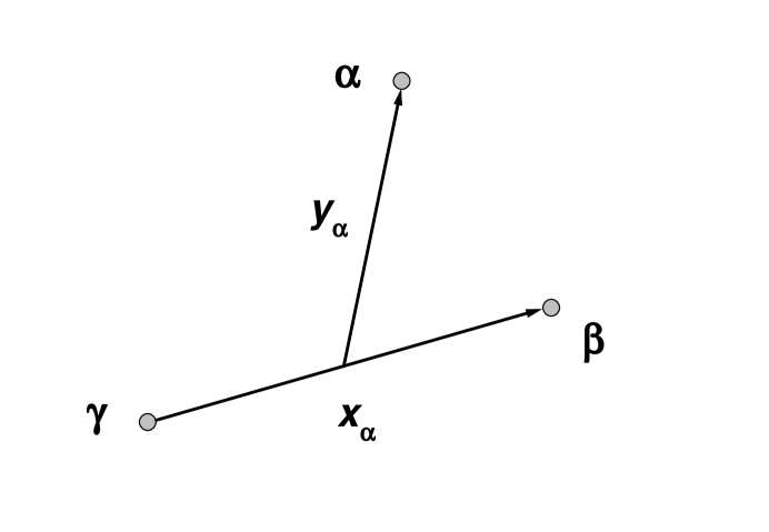
Figure 1: The Jacobi coordinates of the three-body system.

We are going to solve a 3N Schrödinger equation with the c.m. energy $E$,

$$H\Psi=E\Psi,$$ (5)

to obtain the scattering state $\Psi$ initiated by a state $\Xi_{1}$,

$$\langle\vec{x}_{1},\vec{y}_{1}|\Xi_{1}\rangle=\phi^{d}(\vec{x}_{1})F(\vec{y}_{1};\vec{p}_{0}),$$ (6)

where $\phi^{d}(\vec{x}_{1})$ is the deuteron state function of the pair $(2,3)$, and $F(\vec{y}_{1};\vec{p}_{0})$ is a free state function of the nucleon 1 with the momentum $\vec{p}_{0}$. These functions satisfy the following Schrödinger equations,

$$\left[T_{x}(\vec{x}_{1})+V_{1}(\vec{x}_{1})\right]\phi^{d}(\vec{x}_{1})=E_{d}\phi^{d}(\vec{x}_{1}),$$ (7)

and

$$T_{y}(\vec{y}_{1})F(\vec{y_{1}};\vec{p}_{0})=E_{p_{0}}F(\vec{y_{1}};\vec{p}_{0})=\frac{3\hbar^{2}}{4m}p_{0}^{2}F(\vec{y}_{1};\vec{p}_{0}),$$ (8)

with

$$E=E_{d}+E_{p_{0}}.$$ (9)

In a time-independent formal scattering theory, the scattering state is given as

$$\Psi\equiv\lim_{\varepsilon\to 0}\imath\varepsilon G(E+\imath\varepsilon)\Xi_{1}=\lim_{\varepsilon\to 0}\Psi(\varepsilon),$$ (10)

where $G(z)$ is the total three-body Green’s function,

$$G(z)\equiv\frac{1}{z-H_{0}-V}.$$ (11)

Using the free Green’s function, $G_{0}(z)$,

$$G_{0}(z)=\frac{1}{z-H_{0}},$$ (12)

and the resolvent relation,

$$G(z)=G_{0}(z)+G_{0}(z)VG(z),$$ (13)

we obtain

$$\Psi(\varepsilon)=\imath\varepsilon G_{0}(E+\imath\varepsilon)\Xi_{1}+G_{0}(E+\imath\varepsilon)V\Psi(\varepsilon).$$ (14)

In the Faddeev theory with short-range potentials, the three-body state is divided into three components (Faddeev components),

$$\Psi(\varepsilon)=\Phi_{1}(\varepsilon)+\Phi_{2}(\varepsilon)+\Phi_{3}(\varepsilon),$$ (15)

where the Faddeev components are defined as

$$\Phi_{\alpha}(\varepsilon)\equiv\imath\varepsilon G_{0}(E+\imath\varepsilon)\Xi_{1}~{}\delta_{\alpha,1}+G_{0}(E+\imath\varepsilon)V_{\alpha}\Psi(\varepsilon).$$ (16)

Eqs. (15) and (16) give

$$\Phi_{\alpha}(\varepsilon)=\imath\varepsilon G_{\alpha}(E+\imath\varepsilon)\Xi_{1}~{}\delta_{\alpha,1}+G_{\alpha}(E+\imath\varepsilon)V_{\alpha}\left(\Phi_{\beta}(\varepsilon)+\Phi_{\gamma}(\varepsilon)\right),$$ (17)

where we have defined the channel Green’s function $G_{\alpha}(z)$,

$$G_{\alpha}(z)\equiv\frac{1}{z-H_{0}-V_{\alpha}}=\frac{1}{1-G_{0}(z)V_{\alpha}}G_{0}(z).$$ (18)

By taking the $\varepsilon$-limit in Eq. (17), we reach the Faddeev equation,

$$\Phi_{\alpha}\equiv\lim_{\varepsilon\to 0}\Phi_{\alpha}(\varepsilon)=\Xi_{1}~{}\delta_{\alpha,1}+G_{\alpha}(E+\imath 0)V_{\alpha}\left(\Phi_{\beta}+\Phi_{\gamma}\right).$$ (19)

However, the right hand side of Eq. (19) includes the following term,

$$G_{0}(E+\imath 0)v^{c}_{\alpha}(\Phi_{\beta}+\Phi_{\gamma}),$$ (20)

which is known to cause a severe singularity due to the long-range Coulomb force, $v^{c}_{\alpha}(x_{\alpha})$.

2.2 The Coulomb-Modified Faddeev Equation

The singularity in the kernel of the Faddeev equation (19) occurs due to the long-rangeness of the Coulomb interaction $v^{c}_{\alpha}(x_{\alpha})$. We therefore consider to introduce an auxiliary potential that cancels the long-rangeness of $v^{c}_{\alpha}(x_{\alpha})$ for a large $x_{\alpha}$. For this purpose, we define a Coulomb potential $u^{c}_{\beta,\gamma}(y_{\beta})$ that acts between the c.m. of the pair $(\gamma,\alpha)$ and the spectator $\beta$ with respect to the charges of the pair $(\beta,\gamma)$ (see Fig. 2),

$$u^{c}_{\beta,\gamma}(y_{\beta})=\frac{Z_{\beta}Z_{\gamma}e^{2}}{y_{\beta}}.$$ (21)

Using an expression,

$$\vec{y}_{\beta}=\vec{x}_{\alpha}+\frac{1}{2}\vec{x}_{\beta},$$ (22)

which is easily given with the definition of the Jacobi coordinates, Eq. (1), we can show that

$$\frac{1}{x_{\alpha}}-\frac{1}{y_{\beta}}=\frac{1}{x_{\alpha}}-\frac{1}{|\vec{x}_{\alpha}+\frac{1}{2}\vec{x}_{\beta}|}\rightarrow O(x_{\alpha}^{-2}),$$ (23)

when $x_{\alpha}$ becomes large with keeping $x_{\beta}$ finite. The finiteness of $x_{\beta}$ is implicit in a Faddeev component $\Phi_{\beta}$, because the pair $(\gamma,\alpha)$ is in the deuteron bound state or in a closed channel as far as we stay at energies below the three-body breakup threshold. (See the redefinition of the Faddeev component below, Eq. (33).) The range of $v^{c}_{\alpha}(x_{\alpha})-u^{c}_{\beta,\gamma}(y_{\beta})$ is therefore short if it is combined with $\Phi_{\beta}$, i.e.

$$\left\{v^{c}_{\alpha}(x_{\alpha})-u^{c}_{\beta,\gamma}(y_{\beta})\right\}\Phi_{\beta}=Z_{\beta}Z_{\gamma}e^{2}\left(\frac{1}{x_{\alpha}}-\frac{1}{y_{\beta}}\right)\Phi_{\beta}\rightarrow Z_{\beta}Z_{\gamma}e^{2}O(x_{\alpha}^{-2})\Phi_{\beta}.$$ (24)

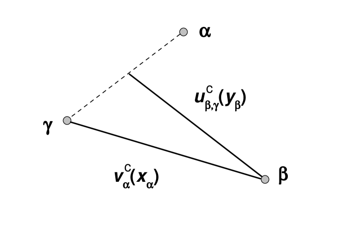
Figure 2: Relation between the Coulomb potential $v^{c}_{\alpha}(x_{\alpha})$ and the auxiliary Coulomb potential $u^{c}_{\beta,\gamma}(y_{\beta})$, which acts between the spectator $\beta$ and the c.m. of the pair $(\gamma,\alpha)$.

With this idea, we write the second term on the right hand side of Eq. (14) as follows:

$$G_{0}(E+\imath\varepsilon)V\Psi(\varepsilon) = G_{0}(E+\imath\varepsilon)\biggl{\{}V_{1}\Phi_{1}(\varepsilon)+V_{2}\Phi_{2}(\varepsilon)+V_{3}\Phi_{3}(\varepsilon)\biggr{\}}$$ (29)

$$+G_{0}(E+\imath\varepsilon)\biggl{\{}\left(V_{1}-u^{c}_{2,3}\right)\Phi_{2}(\varepsilon)+\left(V_{1}-u^{c}_{3,2}\right)\Phi_{3}(\varepsilon)\biggr{\}}$$

$$+G_{0}(E+\imath\varepsilon)\biggl{\{}\left(V_{2}-u^{c}_{3,1}\right)\Phi_{3}(\varepsilon)+\left(V_{2}-u^{c}_{1,3}\right)\Phi_{1}(\varepsilon)\biggr{\}}$$

$$+G_{0}(E+\imath\varepsilon)\biggl{\{}\left(V_{3}-u^{c}_{1,2}\right)\Phi_{1}(\varepsilon)+\left(V_{3}-u^{c}_{2,1}\right)\Phi_{2}(\varepsilon)\biggr{\}}$$

$$+G_{0}(E+\imath\varepsilon)\biggl{\{}u^{c}_{1}\Phi_{1}(\varepsilon)+u^{c}_{2}\Phi_{2}(\varepsilon)+u^{c}_{3}\Phi_{3}(\varepsilon)\biggr{\}},$$

where the last term on the right hand side including a potential $u^{c}_{\alpha}$, which is defined as a two-body Coulomb interaction between the pair $(\beta,\gamma)$ and the spectator $\alpha$,

$$u^{c}_{\alpha}=u^{c}_{\alpha}(y_{\alpha})=u^{c}_{\alpha,\beta}(y_{\alpha})+u^{c}_{\alpha,\gamma}(y_{\alpha})=\frac{Z_{\alpha}(Z_{\beta}+Z_{\gamma})e^{2}}{y_{\alpha}},$$ (30)

is added to compensate the advisedly subtracted terms with $u^{c}_{\alpha,\beta}$’s.

We correspondingly redefine the Faddeev components instead of Eq. (16) as

$$\Phi_{\alpha}(\varepsilon) \equiv \imath\varepsilon G_{0}(E+\imath\varepsilon)\Xi_{1}~{}\delta_{\alpha,1}+G_{0}(E+\imath\varepsilon)(V_{\alpha}+u^{c}_{\alpha})\Phi_{\alpha}(\varepsilon)$$ (33)

$$+G_{0}(E+\imath\varepsilon)\left(V_{\alpha}-u^{c}_{\beta,\gamma}\right)\Phi_{\beta}(\varepsilon)$$

$$+G_{0}(E+\imath\varepsilon)\left(V_{\alpha}-u^{c}_{\gamma,\beta}\right)\Phi_{\gamma}(\varepsilon),$$

which gives

$$\Phi_{\alpha}(\varepsilon) = \imath\varepsilon{\cal G}_{\alpha}(E+\imath\varepsilon)\Xi_{1}~{}\delta_{\alpha,1}+{\cal G}_{\alpha}(E+\imath\varepsilon)\left(V_{\alpha}-u^{c}_{\beta,\gamma}\right)\Phi_{\beta}(\varepsilon)$$ (35)

$$+{\cal G}_{\alpha}(E+\imath\varepsilon)\left(V_{\alpha}-u^{c}_{\gamma,\beta}\right)\Phi_{\gamma}(\varepsilon),$$

where we have defined the channel Coulomb Green’s function ${\cal G}_{\alpha}(z)$ as

$${\cal G}_{\alpha}(z)\equiv\frac{1}{z-H_{0}-V_{\alpha}-u^{c}_{\alpha}}=\frac{1}{1-G_{0}(z)(V_{\alpha}+u^{c}_{\alpha})}G_{0}(z).$$ (36)

Taking the $\varepsilon$-limit in Eq. (35) and using a relation,

$$\lim_{\varepsilon\to 0}\imath\varepsilon\langle\vec{x}_{1},\vec{y}_{1}|{\cal G}_{1}(E+\imath\varepsilon)\Xi_{1}\rangle=\phi^{d}(\vec{x}_{1})F^{c}(\vec{y}_{1};\vec{p}_{0},\eta_{1}),$$ (37)

where $F^{c}(\vec{y}_{1};\vec{p}_{0},\eta_{1})$ is a scattering function in the Coulomb potential $u^{c}_{1}(y_{1})$,

$$\left[T_{y}(\vec{y}_{1})+u^{c}_{1}(y_{1})\right]F^{c}(\vec{y}_{1};\vec{p}_{0},\eta_{1})=\frac{3\hbar^{2}}{4m}p_{0}^{2}F^{c}(\vec{y}_{1};\vec{p}_{0},\eta_{1}),$$ (38)

and $\eta_{\alpha}$ is the Coulomb parameter,

$$\eta_{\alpha}=\frac{2m}{3\hbar^{2}}\frac{Z_{\alpha}(Z_{\beta}+Z_{\gamma})e^{2}}{p_{0}},$$ (39)

we get the Coulomb-modified Faddeev equation,

$$\Phi_{\alpha} = \phi^{d}F^{c}(\vec{p}_{0},\eta_{1})~{}\delta_{\alpha,1}+{\cal G}_{\alpha}(E+\imath 0)\left(V_{\alpha}-u^{c}_{\beta,\gamma}\right)\Phi_{\beta}$$ (41)

$$+{\cal G}_{\alpha}(E+\imath 0)\left(V_{\alpha}-u^{c}_{\gamma,\beta}\right)\Phi_{\gamma}.$$

Since the potential term $V_{\alpha}-u^{c}_{\beta,\gamma}$ is a short-range interaction with respect to $|\vec{x}_{\alpha}|$ as mentioned above, Eq. (41) can be treated as in the $nd$ problem. At the same time, it is noted that the appearance of the channel Coulomb Green’s function ${\cal G}_{\alpha}(E+\imath 0)$ expresses that the spectator particle is distorted by the long-range Coulomb force. In the original idea of the Faddeev theory with a short-range interaction, while pair particles are interacting, the spectator particle is considered to be free. This picture is no more valid with the Coulomb force, and the auxiliary Coulomb potential creates the Coulomb wave function that expresses the distortion.

For the case of identical particles, the initial state should be

$$\Xi=\Xi_{1}+\Xi_{2}+\Xi_{3}.$$ (42)

In this case, each Faddeev component has the same functional form and satisfies the same equation,

$$\Phi_{\alpha}=\phi^{d}F^{c}(\vec{p}_{0},\eta_{\alpha})+{\cal G}_{\alpha}(E+\imath 0)\left\{[V_{\alpha}-u^{c}_{\beta,\gamma}]\Phi_{\beta}+[V_{\alpha}-u^{c}_{\gamma,\beta}]\Phi_{\gamma}\right\}.$$ (43)

2.3 Elastic Singularity and Elastic Amplitude

In this subsection, we derive an expression for the elastic amplitude for the $pd$ scattering below three-body breakup threshold. For this, we write the Coulomb-modified Faddeev equation (43) as

$$\Phi_{1}=\phi^{d}F^{c}(\vec{p}_{0},\eta_{1})+{\cal G}_{1}\Delta_{1}\Phi_{1},$$ (44)

where the operator $\Delta_{1}$ involves a coordinate transformation,

$$\Delta_{1}\Phi_{1}\equiv\left(V_{1}-u^{c}_{2,3}\right)\Phi_{2}+\left(V_{1}-u^{c}_{3,2}\right)\Phi_{3}.$$ (45)

Hereafter, we drop the particle number for simplicity. In the case of the scattering problem, the Green’s function ${\cal G}$ possesses a pole corresponding to the deuteron bound state. In order to treat this pole, we apply a subtraction method, in which we insert an identity,

$$1=|\phi^{d})(\phi^{d}|+\left[1-|\phi^{d})(\phi^{d}|\right],$$ (46)

between ${\cal G}$ and $\Delta$ in Eq. (44) to obtain

$$\langle\vec{x},\vec{y}|\Phi\rangle=\phi^{d}(\vec{x})F^{c}(\vec{y};\vec{p}_{0},\eta)+\phi^{d}(\vec{x})\langle\vec{y}|\breve{G}_{c}(\phi^{d}|\Delta\Phi\rangle+\langle\vec{x},\vec{y}|\Gamma\Delta\Phi\rangle.$$ (47)

Here, $\breve{G}_{c}$ is the Coulomb Green’s function for the outgoing particle,

$$\breve{G}_{c}\equiv\frac{1}{E_{p_{0}}+\imath\varepsilon-T_{y}(\vec{y})-u^{c}(y)},$$ (48)

whose analytical form is known [29] as

$$\langle\vec{y}|\breve{G}_{c}|\vec{y}^{\prime}\rangle=\sum_{\ell,m}Y_{\ell}^{m}(\hat{y})\breve{G}_{c,\ell}^{(+)}(y,y^{\prime})Y_{\ell}^{m\ast}(\hat{y}^{\prime}),$$ (49)

and

$$\breve{G}_{c,\ell}^{(+)}(y,y^{\prime})=-\frac{4m}{3\hbar^{2}}p_{0}e^{\imath\sigma_{\ell}}\frac{u^{(+)}_{\ell}(p_{0}y_{>})}{p_{0}y_{>}}\frac{F_{\ell}(p_{0}y_{<})}{p_{0}y_{<}},$$ (50)

where $F_{\ell}(r)$ is the (real) regular Coulomb function, $u^{(+)}_{\ell}(p_{0}y)$ is defined with the (real) irregular Coulomb function $G_{\ell}(r)$ as

$$u^{(+)}_{\ell}(p_{0}y)=e^{-\imath\sigma_{\ell}}\left(F_{\ell}(p_{0}y)+\imath G_{\ell}(p_{0}y)\right),$$ (51)

and $\sigma_{\ell}$ is the Coulomb phase shift,

$$\sigma_{\ell}={\rm arg}\Gamma(\ell+1+\imath\eta).$$ (52)

The operator $\Gamma$ is

$$\Gamma \equiv \frac{1}{E+\imath\varepsilon-H_{0}-V(\vec{x})-u^{c}(y)}\left[1-|\phi^{d})(\phi^{d}|\right]$$ (53)

$$= \int d\vec{p}|F^{c}(\vec{p},\eta)\rangle\left\{\frac{1}{E_{q}+\imath\varepsilon-T_{x}(\vec{x})-V(\vec{x})}-\frac{|\phi^{d})(\phi^{d}|}{E_{q}-E_{d}}\right\}\langle F^{c}(\vec{p},\eta)|,$$ (54)

where $E_{q}$ is the energy of the two-body subsystem,

$$E_{q}=E-\frac{3\hbar^{2}}{4m}p^{2}=\frac{\hbar^{2}}{m}q^{2},$$ (56)

and $F^{c}(\vec{p},\eta)$ is the Coulomb-modified spectator state, which is a solution of Eq. (38) with the eigenvalue of $\frac{3\hbar^{2}}{4m}p^{2}$. Because the singularities in the first and second terms on the right hand side in Eq. (LABEL:eq:Gamma) cancel each other, we can apply the standard quadrature to perform the $p$-integration in Eq. (LABEL:eq:Gamma) if both terms are treated together.

The first and second terms on the right hand side of Eq. (47) may be considered as a state that describes the elastic scattering. We correspondingly define a elastic function, ${\cal F}^{el}(\vec{y})$, as

$${\cal F}^{el}(\vec{y})\equiv F^{c}(\vec{y};\vec{p}_{0},\eta)+\langle\vec{y}|\breve{G}_{c}(\phi^{d}|\Delta\Phi\rangle.$$ (57)

Substituting a formal solution of Eq. (47) for $\Phi$ to the second term on the right hand side of Eq. (57), we obtain the following equation,

$${\cal F}^{el}(\vec{y})=F^{c}(\vec{y};\vec{p}_{0},\eta)+\langle\vec{y}|\breve{G}_{c}(\phi^{d}|\Delta\frac{1}{1-\Gamma\Delta}\phi^{d}{\cal F}^{el}\rangle.$$ (58)

Although the interaction term in Eq. (58) is very complicated because of the coordinate transformation operator $\Delta$, this equation has the same form as the Lippmann-Schwinger equation for a two-body scattering problem with a short-range force and the Coulomb force. As in the case of the two-body problem, using the explicit form of the Green’s function $\breve{G}_{c}$, Eqs. (49) and (50), the asymptotic form of the function $u^{(+)}_{\ell}(p_{0}y)$,

$$u^{(+)}_{\ell}(p_{0}y)|_{y\to\infty}=\exp\left(+\imath(p_{0}y-\eta\ln 2p_{0}y-\ell\pi/2)\right),$$ (59)

and the decomposition of the Coulomb scattering function $F^{c}(\vec{y};\vec{p}_{0},\eta)$,

$$F^{c}(\vec{y};\vec{p}_{0},\eta)=4\pi\sum_{\ell,m}\imath^{\ell}Y_{\ell}^{m*}(\hat{p_{0}})Y_{\ell}^{m}(\hat{y})e^{\imath\sigma_{\ell}}\frac{F_{\ell}(p_{0}y)}{p_{0}y},$$ (60)

we obtain an asymptotic form of the elastic wave function ${\cal F}^{el}(\vec{y})$,

$${\cal F}^{el}(\vec{y})|_{y\to\infty}=F^{c}(\vec{y};\vec{p}_{0},\eta)+\hat{f}^{el}(\hat{y})\frac{e^{\imath(p_{0}y-\eta\ln 2p_{0}y)}}{y},$$ (61)

where $\hat{f}^{el}(\hat{y})$ is defined as

$$\hat{f}^{el}(\hat{y})=-\frac{3\hbar^{2}}{4m}\frac{1}{4\pi}\langle\overline{F^{c}}(p_{0}\hat{y},\eta)\phi^{d}|\Delta\Phi\rangle.$$ (62)

The scattering amplitude of the elastic scattering is therefore given as

$$f(\hat{y})=f^{c}(\hat{y})+\hat{f}^{el}(\hat{y}),$$ (63)

where $f^{c}(\hat{y})$ is the pure Coulomb scattering amplitude,

$$f^{c}(\hat{y})=-\frac{\eta}{2p_{0}\sin^{2}\theta/2}e^{-\imath\eta\ln(\sin^{2}\theta/2)+2\imath\sigma_{0}}.$$ (64)

3 Numerical Results

3.1 Some Remarks on Numerical Methods

In this section, we present some results of our calculations to solve the Coulomb-modified Faddeev equation (44) for the $pd$ scattering problem at energies below the three-body breakup threshold. Although techniques used in the numerical calculations are essentially the same with those in the 3N bound state studies [14, 16, 17, 18], we give some remarks in this subsection.

We solve the Coulomb-modified Faddeev equation (44) with an iterative method, which is called as the Method of Continued Fractions [17, 18]. In most iterative methods to solve a linear integral equation, a $k$-th order process involves the calculation of a function $\Pi$ given by operating the integral kernel to a known function $\Omega$ that is produced from the $(k-1)$-th order solution. In the present case, we have

$$\Pi(\vec{x},\vec{y})\equiv\langle\vec{x},\vec{y}|{\cal G}\Delta\Omega\rangle=\phi^{d}(\vec{x})\langle\vec{y}|\breve{G}_{c}(\phi^{d}|\Delta\Omega\rangle+\langle\vec{x},\vec{y}|\Gamma\Delta\Omega\rangle.$$ (65)

The first term on the right hand side of Eq. (65) is calculated numerically using the explicit expression of the Green’s function $\breve{G}_{c}$, Eqs. (49) and (50).

From the definition of the $\Gamma$-operator, Eq. (LABEL:eq:Gamma), the second term on the right hand side of Eq. (65) reads

$$\langle\vec{x},\vec{y}|\Gamma\Delta|\Omega\rangle=\int d\vec{p}F^{c}(\vec{y};\vec{p},\eta)\left\{\Theta(\vec{x};\vec{p})-\phi^{d}(\vec{x})C(\vec{p})\right\},$$ (66)

where $C(\vec{p})$ is given by

$$C(\vec{p})=\frac{1}{E_{q}-E_{d}}\langle\phi^{d}F^{c}(\vec{p},\eta)|\Delta\Omega\rangle,$$ (67)

and $\Theta(\vec{x};\vec{p})$ by

$$\Theta(\vec{x};\vec{p})=\frac{1}{E_{q}+\imath\varepsilon-T_{x}(\vec{x})-V(\vec{x})}(F^{c}(\vec{p},\eta)|\Delta\Omega\rangle.$$ (68)

In actual numerical calculations, this $\Theta(\vec{x};\vec{p})$ is obtained as a solution of Schrödinger-like differential equation,

$$\left[E_{q}-T_{x}(\vec{x})-V(\vec{x})\right]\Theta(\vec{x};\vec{p})=(F^{c}(\vec{p},\eta)|\Delta\Omega\rangle,$$ (69)

with the boundary condition that $\Theta(\vec{x};\vec{p})$ vanishes at a large $x$ because $E_{q}$ is negative in the present case. (See Eq. (56).) After a decomposition of $\Theta(\vec{x};\vec{p})$ into partial waves, we have a set of ordinary differential equation, whose solutions can be obtained with the usual technique as in the two-body problem.

For the partial-wave decomposition, we use the following angular-spin-isospin functions in the $J-j$ coupling scheme,

$$\left|{}^{2S+1}L_{J},\ell_{j};J_{0}^{\pi}M_{0}\right)\left|IM_{I},\frac{1}{2}\mu;M_{T}\right),$$ (70)

where $L$ is the relative orbital angular momentum of the pair nucleons; $S$ the total spin of the pair; $J$ the total angular momentum of the pair ($\vec{J}=\vec{L}+\vec{S}$); $\ell$ the orbital angular momentum of the spectator nucleon; $j$ the sum of $\ell$ and the spin of the spectator ($\vec{j}=\vec{\ell}+\vec{\frac{1}{2}}$); $J_{0}$ and $M_{0}$ the total angular momentum of the three nucleons ($\vec{J}_{0}=\vec{J}+\vec{j}$) and its third component, respectively; $\pi$ the parity of the system (= $(-)^{L+\ell}$); $I$ and $M_{I}$ the total isospin and its third component of the pair; $\mu$ the third component of the isospin of the spectator; $M_{T}$ the third component of the total isospin of the three nucleons ($M_{T}=+\frac{1}{2}$ for the $pd$ scattering and $M_{T}=-\frac{1}{2}$ for the $nd$ scattering). Note that we use the isospin function in which the isotriplet pair nucleons are assigned as proton-proton (neutron-neutron) for $M_{I}=+1(-1)$ and proton-neutron for $M_{I}=0$. With this form, we take into account the mixing of the total isospin, $1/2$ and $3/2$, arising from the inclusion of the Coulomb force and/or a charge symmetry breaking (CSB) NN forces. Actual form of the isospin functions, whose phases are chosen for convenience’ sake in the coordinate transformation, is shown in Table 1 [14, 16].

In the present calculation, 3N partial-wave states for which NN force acts are restricted to those with total two-nucleon angular momenta $J\leq 3$ (see Subsect. 3.2), and the total 3N angular momentum $J_{0}$ is truncated at $J_{0}=19/2$ in calculating scattering observables in Subsects. 3.3 and 3.4.

Table 1: Three-nucleon isospin functions for $M_{T}=\pm\frac{1}{2}$.

	$I$	$M_{I}$	$\mu$	$|IM_{I},\frac{1}{2}\mu;M_{T})$
#0	0	0	$\pm\frac{1}{2}$	$\pm|00)|\frac{1}{2}\pm\frac{1}{2})$
#1	1	0	$\pm\frac{1}{2}$	$-|10)|\frac{1}{2}\pm\frac{1}{2})$
#2	1	$\pm 1$	$\mp\frac{1}{2}$	$|1\pm 1)|\frac{1}{2}\mp\frac{1}{2})$

3.2 Phase Shift Parameters

As a first step, we use the Malfliet-Tjon (MT) I-III NN potential [30] with parameters given in ref. [31]. Because of the simplicity that the MT I-III potential acts only on the spin triplet and the spin singlet $S$-wave NN states, the $S$-wave nucleon-deuteron ($Nd$) elastic channel is classified only by the channel spin: the sum of the nucleon spin and the deuteron spin, namely, $1/2$ (the doublet state) or $3/2$ (the quartet state). In Table 2, calculated $S$-wave phase shifts of the doublet (${}^{2}\delta$) and the quartet (${}^{4}\delta$) states for $Nd$ elastic scattering at some energies below the three-body breakup threshold are compared with the results of the configuration-space Faddeev calculations [23], whose results for a realistic NN potential model, the Argonne V₁₄ model (AV14) [32], were published as benchmarks [33] in the $pd$ calculation.

The differences between our calculations and those of ref. [23] are an order of 1% at every energies.

Table 2: The $nd$ and $pd$ $S$-wave phase shifts with for the MT I-III potential. The phase shifts are in degrees.

	${}^{2}\delta_{nd}$		${}^{4}\delta_{nd}$
	—————————–		—————————–
$E_{n}^{\mathrm{Lab}}$ (MeV)	Ref. [23]	This work	Ref. [23]	This work
0.0015	-0.230	-0.228	-2.09	-2.09
0.15	-3.28	-3.26	-20.4	-20.5
1.5	-20.7	-20.6	-55.8	-55.9
2.45	-28.6	-28.6	-66.7	-66.7
3.27	-33.6	-33.4	-73.6	-73.5
	${}^{2}\delta_{pd}$		${}^{4}\delta_{pd}$
	—————————–		—————————–
$E_{p}^{\mathrm{Lab}}$ (MeV)	Ref. [23]	This work	Ref. [23]	This work
0.15	-0.537	-0.527	-7.46	-7.44
1.0	-10.6	-10.5	-37.7	-37.2
1.5	-16.2	-16.2	-46.5	-46.4
2.0	-21.1	-21.0	-53.5	-53.3
3.0	-28.8	-28.7	-63.8	-63.4

Next, we examine our calculations with a more realistic NN potential, the Argonne V₁₈ model (AV18) [34]. We follow the convention of the phase shifts and mixing parameters in ref. [35], where the $Nd$ elastic channel is denoted as ${}^{2K+1}\ell_{J_{0}}$ with $K$ being the channel spin ($\vec{K}=\vec{1}+\vec{\frac{1}{2}}$, $\vec{J}_{0}=\vec{K}+\vec{\ell}$). These parameters are calculated with partial-wave amplitudes in the channel spin scheme, which are transformed from our partial-wave amplitudes in the $J-j$ coupling scheme in a trivial manner [35]. In Tables 3 and 4, we present results of the phase shift parameters up to $J_{0}=5/2$ at $E_{N}^{\mathrm{Lab}}=1$ MeV and $E_{N}^{\mathrm{Lab}}=3$ MeV, respectively. In the tables, our calculations with $J\leq 2(3)$ are denoted as $J_{\mathrm{max}}=2(3)$. The results are compared with those of the variational method with the PHH basis [27, 28], whose results for the AV14 potential were also published as the benchmarks [35, 33]. From these tables, we see that our calculations almost converge at $J_{\mathrm{max}}=3$ and the differences from the PHH calculations are again order of 1%. In addition, although results are not shown in the tables, we have examined the convergence of the partial-wave expansion of the term $v^{c}_{\alpha}(x_{\alpha})-u^{c}_{\beta,\gamma}(y_{\beta})$ in Eq. (43) by neglecting $J=3$ NN force components $v^{s}_{\alpha}(x_{\alpha})$ in the $J_{\mathrm{max}}=3$ calculation. The discrepancies between the results and the $J_{\mathrm{max}}=2$ calculations are much less than 1%, which shows that the effect of the $J=3$ components in the term $v^{c}_{\alpha}(x_{\alpha})-u^{c}_{\beta,\gamma}(y_{\beta})$ is negligibly small.

Tables 2, 3, and 4 demonstrate that our formalism gives quite promising results in calculating the $nd$ and $pd$ elastic scattering at low energies.

Table 3: The $nd$ and $pd$ phase shifts parameters at $E_{N}^{\mathrm{Lab}}=1$ MeV with AV18 potential. The PHH results are taken from ref. [28]. Values of all parameters are in degrees.

		$nd$			$pd$
		——————————————			——————————————
		This work		PHH	This work		PHH
$J_{0}^{\pi}$		$J_{\mathrm{max}}=2$	$J_{\mathrm{max}}=3$		$J_{\mathrm{max}}=2$	$J_{\mathrm{max}}=3$
$\frac{1}{2}^{+}$	${}^{4}D_{1/2}$	-0.99	-0.99	-0.98	-0.770	-0.770	-0.771
	${}^{2}S_{1/2}$	-18.5	-18.1	-18.1	-13.8	-13.5	-13.2
	$\eta_{1/2+}$	0.875	0.919	0.928	0.93	0.98	1.02
$\frac{1}{2}^{-}$	${}^{2}P_{1/2}$	-4.13	-4.15	-4.13	-3.32	-3.33	-3.34
	${}^{4}P_{1/2}$	12.1	12.1	12.0	8.98	8.95	9.19
	$\varepsilon_{1/2-}$	3.46	3.44	3.47	2.96	2.95	2.89
$\frac{3}{2}^{+}$	${}^{4}S_{3/2}$	-46.9	-46.9	-46.7	-36.9	-36.9	-37.0
	${}^{2}D_{3/2}$	0.572	0.571	0.564	0.432	0.431	0.442
	${}^{4}D_{3/2}$	-1.06	-1.06	-1.05	-0.821	-0.823	-0.829
	$\varepsilon_{3/2+}$	0.607	0.606	0.621	0.628	0.613	0.784
	$\zeta_{3/2+}$	0.516	0.515	0.511	0.493	0.493	0.500
	$\eta_{3/2+}$	-0.110	-0.107	-0.107	-0.093	-0.091	-0.089
$\frac{3}{2}^{-}$	${}^{4}F_{3/2}$	0.124	0.124	0.121	0.095	0.095	0.097
	${}^{2}P_{3/2}$	-4.08	-4.09	-4.08	-3.29	-3.29	-3.30
	${}^{4}P_{3/2}$	14.0	14.0	13.9	10.5	10.4	10.7
	$\varepsilon_{3/2-}$	-1.24	-1.28	-1.24	-1.05	-1.08	-1.02
	$\zeta_{3/2-}$	-0.173	-0.177	-0.177	-0.184	-0.187	-0.182
	$\eta_{3/2-}$	-1.05	-1.04	-1.04	-0.968	-0.961	-0.932
$\frac{5}{2}^{+}$	${}^{4}G_{5/2}$	-0.015	-0.015	-0.015	-0.011	-0.012	-0.011
	${}^{2}D_{5/2}$	0.568	0.567	0.560	0.429	0.428	0.439
	${}^{4}D_{5/2}$	-1.12	-1.12	-1.11	-0.869	-0.871	-0.879
	$\varepsilon_{5/2+}$	-0.276	-0.265	-0.277	-0.272	-0.249	-0.364
	$\zeta_{5/2+}$	-0.273	-0.270	-0.272	-0.272	-0.270	-0.300
	$\eta_{5/2+}$	-0.810	-0.818	-0.821	-0.818	-0.824	-0.943
$\frac{5}{2}^{-}$	${}^{4}P_{5/2}$	13.3	13.2	13.2	9.9	9.8	10.0
	${}^{2}F_{5/2}$	-0.064	-0.064	-0.063	-0.049	-0.049	-0.049
	${}^{4}F_{5/2}$	0.129	0.129	0.127	0.099	0.099	0.100
	$\varepsilon_{5/2-}$	0.441	0.443	0.447	0.414	0.419	-0.218
	$\zeta_{5/2-}$	0.383	0.390	0.390	0.385	0.391	0.384
	$\eta_{5/2-}$	-0.120	-0.123	-0.123	-0.120	-0.122	-0.127

Table 4: The $nd$ and $pd$ phase shifts parameters at $E_{N}^{\mathrm{Lab}}=3$ MeV with AV18 potential. The PHH results are taken from refs. [27, 28]. Values of all parameters are in degrees.

		$nd$			$pd$
		——————————————			——————————————
		This work		PHH	This work		PHH
$J_{0}^{\pi}$		$J_{\mathrm{max}}=2$	$J_{\mathrm{max}}=3$		$J_{\mathrm{max}}=2$	$J_{\mathrm{max}}=3$
$\frac{1}{2}^{+}$	${}^{4}D_{1/2}$	-3.86	-3.87	-3.85	-3.55	-3.56	-3.56
	${}^{2}S_{1/2}$	-35.8	-35.2	-35.3	-32.8	-32.3	-32.2
	$\eta_{1/2+}$	1.03	1.10	1.12	1.02	1.07	1.10
$\frac{1}{2}^{-}$	${}^{2}P_{1/2}$	-7.42	-7.47	-7.49	-7.32	-7.37	-7.36
	${}^{4}P_{1/2}$	24.3	24.2	24. 2	21.8	21.7	22.1
	$\varepsilon_{1/2-}$	6.70	6.67	6.68	5.76	5.74	5.71
$\frac{3}{2}^{+}$	${}^{4}S_{3/2}$	-70.0	-70.1	-69.9	-62.9	-63.0	-63.1
	${}^{2}D_{3/2}$	2.39	2.37	2.36	2.09	2.07	2.15
	${}^{4}D_{3/2}$	-4.15	-4.16	-4.14	-3.81	-3.82	-3.83
	$\varepsilon_{3/2+}$	0.724	0.720	0.747	0.792	0.753	0.800
	$\zeta_{3/2+}$	1.37	1.36	1.35	1.29	1.29	1.30
	$\eta_{3/2+}$	-0.377	-0.363	-0.363	-0.327	-0.320	-0.322
$\frac{3}{2}^{-}$	${}^{4}F_{3/2}$	0.931	0.929	0.920	0.830	0.828	0.849
	${}^{2}P_{3/2}$	-7.10	-7.12	-7.18	-7.08	-7.11	-7.14
	${}^{4}P_{3/2}$	26.1	25.9	26.0	24.0	23.9	24.2
	$\varepsilon_{3/2-}$	-2.63	-2.69	-2.61	-2.24	-2.30	-2.20
	$\zeta_{3/2-}$	-0.245	-0.261	-0.265	-0.305	-0.317	-0.321
	$\eta_{3/2-}$	-3.57	-3.52	-3.52	-3.14	-3.10	-3.11
$\frac{5}{2}^{+}$	${}^{4}G_{5/2}$	-0.208	-0.208	-0.206	-0.189	-0.189	-0.189
	${}^{2}D_{5/2}$	2.36	2.34	2.33	2.07	2.05	2.13
	${}^{4}D_{5/2}$	-4.48	-4.49	-4.46	-4.09	-4.11	-4.13
	$\varepsilon_{5/2+}$	-0.316	-0.285	-0.315	-0.315	-0.257	-0.350
	$\zeta_{5/2+}$	-0.716	-0.693	-0.701	-0.707	-0.688	-0.699
	$\eta_{5/2+}$	-1.97	-2.03	-2.04	-2.04	-2.09	-2.07
$\frac{5}{2}^{-}$	${}^{4}P_{5/2}$	26.2	26.1	26.0	23.8	23.7	23.9
	${}^{2}F_{5/2}$	-0.467	-0.470	-0.466	-0.430	-0.434	-0.433
	${}^{4}F_{5/2}$	0.961	0.957	0.951	0.862	0.858	0.876
	$\varepsilon_{5/2-}$	0.481	0.495	0.538	0.412	0.434	0.343
	$\zeta_{5/2-}$	0.898	0.927	0.926	0.897	0.928	0.932
	$\eta_{5/2-}$	-0.325	-0.340	-0.334	-0.338	-0.349	-0.343

Having established the accuracy of our calculations, we proceed to compare our results with available experimental analysis. In ref. [2], a phase shift analysis (PSA) was performed for the $pd$ scattering at $E_{p}^{\mathrm{Lab}}=3$ MeV, corresponding to $E_{d}^{\mathrm{Lab}}=6$ MeV. Results of our calculations for the phase shift parameters are compared with the PSA results in Table 3.2. The authors in ref. [2] noticed two significant differences of their PSA results from those of Faddeev calculations with the PEST16 NN potential [20]: the ${}^{2}S_{1/2}$ phase shift and the $S-D$ mixing parameter, $\eta_{1/2+}$. The similar differences are observed for the comparison with our AV18 results in Table 3.2. The discrepancy in the ${}^{2}S_{1/2}$ phase shift is related to the binding energy of the 3N bound state. While the experimental value of $\mathrm{}^{3}He$ binding energy is 7.72 MeV, the calculated value for AV18 is 6.91 MeV. To solve this discrepancy, we introduce a 3NF model by Brazil group (BR) [36] based on the two-pion exchange process with the cut-off parameter of 700 MeV. Calculated $\mathrm{}^{3}He$ binding energy for the AV18 plus the BR-3NF (AV18+BR) is 7.79 MeV. At the same time, although not enough but a significant improvement is observed for the ${}^{2}S_{1/2}$ phase shift and the $\eta_{1/2+}$ parameter as shown in Table 3.2.

Table 5: Phase shift parameters for $pd$ scattering at $E_{p}^{\mathrm{Lab}}=3$ MeV calculated for AV18, AV18+BR and AV18+BR+LS1. Values of PSA are taken from ref. [2]. Values of all parameters are in degrees.

		PSA	AV18	AV18+BR	AV18+BR+LS1
$S$-wave phases:
	${}^{4}S_{3/2}$	-63.95$\pm$0.28	-63.01	-63.02	-63.02
	${}^{2}S_{1/2}$	-24.87$\pm$0.35	-32.29	-27.35	-27.43
$P$-wave phases:
	${}^{4}P_{J_{0}}$ average	23.37$\pm$0.11	23.09	23.29	23.19
	${}^{4}P_{5/2}-{}^{4}P_{3/2}$	0.01$\pm$0.06	-0.17	0.04	0.40
	${}^{4}P_{3/2}-{}^{4}P_{1/2}$	2.49$\pm$0.11	2.17	1.88	2.18
	${}^{2}P_{J_{0}}$ average	-7.11$\pm$0.24	-7.24	-7.24	-7.26
	${}^{2}P_{3/2}-{}^{2}P_{1/2}$	-0.14$\pm$0.25	0.26	0.29	0.34
$D$-wave phases:
	${}^{4}D_{J_{0}}$ average	-3.74$\pm$0.01	-3.81	-3.81	-3.81
	${}^{4}D_{7/2}-{}^{4}D_{5/2}$	0.31$\pm$0.03	0.37	0.37	0.38
	${}^{4}D_{5/2}-{}^{4}D_{3/2}$	-0.28$\pm$0.03	-0.29	-0.29	-0.28
	${}^{4}D_{3/2}-{}^{4}D_{1/2}$	-0.16$\pm$0.03	-0.26	-0.27	-0.27
	${}^{2}D_{J_{0}}$ average	1.99$\pm$0.09	2.06	2.06	2.06
	${}^{2}D_{5/2}-{}^{2}D_{3/2}$	0.0 (fixed)	-0.02	-0.02	-0.02
$S-D$ mixing parameters:
	$\eta_{1/2+}$	2.00$\pm$0.10	1.07	1.51	1.50
	$\zeta_{3/2+}$	1.20$\pm$0.04	1.29	1.29	1.29
	$\eta_{3/2+}$	-0.28$\pm$0.03	-0.32	-0.31	-0.31
$P-P$ mixing parameters:
	$\varepsilon_{1/2-}$	5.73$\pm$0.13	5.74	5.78	5.69
	$\varepsilon_{3/2-}$	-2.47$\pm$0.05	-2.30	-2.41	-2.52
$P-F$ mixing parameters:
	$\zeta_{3/2-}$	-1.25$\pm$0.54	-0.32	-0.31	-0.30
	$\eta_{3/2-}$	-3.13$\pm$0.23	-3.10	-3.11	-3.12
	$\zeta_{5/2-}$	-0.62$\pm$0.20	0.93	0.92	0.91
	$\eta_{5/2-}$	-0.45$\pm$0.04	-0.35	-0.35	-0.35
$D-D$ mixing parameters:
	$\varepsilon_{3/2+}$	2.15$\pm$0.24	0.75	0.76	0.78
	$\varepsilon_{5/2+}$	-0.75$\pm$0.12	-0.26	-0.26	-0.25

In addition, we observe a significant discrepancy in the splittings of the spin quartet $P$-wave phase shifts, $\delta_{{}^{4}P_{J_{0}}}$ with $J_{0}$ = 1/2, 3/2, and 5/2, although their average for AV18 and AV18+BR agrees with the PSA values. This difference is closely related with so called the $A_{y}(\theta)$ puzzle: calculated values of the nucleon analyzing power $A_{y}(\theta)$ with realistic NN potentials for energies below $\approx$ 30 MeV underestimate systematically from experimental values [37, 38]. In ref. [39], a combination of $P$-wave phase shifts,

$$-4\delta_{{}^{4}P_{1/2}}-5\delta_{{}^{4}P_{3/2}}+9\delta_{{}^{4}P_{5/2}}=4\left(\delta_{{}^{4}P_{3/2}}-\delta_{{}^{4}P_{1/2}}\right)+9\left(\delta_{{}^{4}P_{5/2}}-\delta_{{}^{4}P_{3/2}}\right),$$ (71)

was shown to be a good measure of the height of $A_{y}$-peak. The value of Eq. (71) is 10.05$\pm$0.70 for the PSA values, 7.15 for AV18, and 7.88 for AV18+BR. The values of AV18 and AV18+BR are smaller than the experimental values by about 30%, which is consistent with the underestimation of the $A_{y}$-peak height at 3 MeV. (See Subsect. 3.4.)

Although we do not have any consensus to solve the $A_{y}(\theta)$ puzzle at the moment, one possible reason for the discrepancy might be an unknown three-nucleon force that has a character of spin-orbit forces. In ref. [40], Kievsky introduced purely phenomenological spin-orbit three-nucleon potentials. We take one of the 3NF models that has the longest range (LS1). The binding energy of the $\mathrm{}^{3}He$ for the LS1-3NF in addition to the BR-3NF (AV18+BR+LS1) is 7.77 MeV. Results of the phase shift parameters for AV18+BR+LS1 are also shown in Table 3.2. The LS1-3NF gives a remarkable effect on the phase shift splittings of ${}^{4}P_{J_{0}}$ states. As a result, the value of Eq. (71) for AV18+BR+LS1 is 12.32.

3.3 Differential Cross Sections

In ref. [3], the angular distributions of the differential cross section (DCS) for the $pd$ elastic scattering were measured precisely in the energy range of $2\leq E_{p}^{\mathrm{Lab}}\leq 18$ MeV. In Fig. 3, we plot their results at $E_{p}^{\mathrm{Lab}}=3.0$ MeV being normalized to our theoretical results of the AV18 calculation. We observe that the theoretical results overestimate the experimental data by about 5% at all scattering angles. Similar discrepancy has been observed in recent $pd$ experimental data at low energies [9, 11].

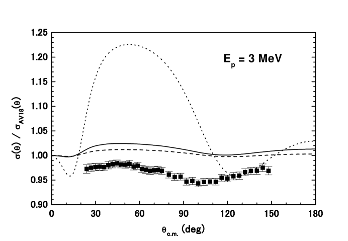
Figure 3: Calculated and experimental $pd$ differential cross sections normalized by the result of the AV18 calculation at $E_{p}^{\mathrm{Lab}}=3.0$ MeV. Dotted curve denote the result of the approximated Coulomb treatment with the AV18 $nd$ calculation. Solid and dashed curves are results with the AV14^′, and dTRS^′ calculations, respectively. Experimental data are taken from ref. [3].

The authors in ref. [3] extracted the cross-section minimum, which appears around $\theta_{\mathrm{c.m.}}=100^{\circ}$, from their data, and compared their results with the prediction of Faddeev calculations with the Paris NN potential, in which the $pd$ scattering amplitudes are approximated as the sum of the $pd$ two-body Rutherford amplitudes and $nd$ Faddeev amplitudes with the $pd$ two-body Coulomb phases as was done in ref. [41]. As a result, they found that the ratio of the theoretical cross-section minimum to the experimental one reveals a strong energy dependence. The theoretical cross-section minimum overestimates the experimental one by about 20% at $E_{p}^{\mathrm{Lab}}=2$ MeV. The overestimation reduces to about 10% at 3 MeV, and once disappears at 5 MeV. At higher energies, the calculations underestimate the experimental one. (See Fig. 17 in ref. [3].) The dotted line in Fig. 3, which denotes the result of AV18 with the same approximation as that in ref. [41], is consistent with the result of ref. [3]. We therefore conclude that the overestimation of DCS at low energies observed in ref. [3] is due to the improper treatment of the Coulomb force, and it is reduced to about 5% by a proper treatment of the Coulomb force.

Besides the AV18 model, we examine some other realistic NN interaction models: a super soft-core model of de Tourreil et al. (dTRS) [42] and the earlier version of the Argonne model, AV14 [32]. Since the isospin-triplet component of these potentials was made as either proton-proton or neutron-proton force, a charge dependence is introduced so as to explain the difference among proton-proton, neutron-proton, and neutron-neutron ${}^{1}S_{0}$ scattering lengths [16]. The results with these models (AV14^′ and dTRS^′) are plotted in Fig.  3. The figure shows that the differences of the DCS due to the different input NN potentials observed at $\theta_{\mathrm{c.m.}}\sim 60^{\circ}$ and $\theta_{\mathrm{c.m.}}\sim 180^{\circ}$ are at most 3%. At $\theta_{\mathrm{c.m.}}\sim 120^{\circ}$, where the dependence on the input NN potentials is small, the calculated results overshoot the experimental data by about 5%.

As is seen in the results of the $pd$ $S$-wave phase shift parameters, we may expect that the introduction of the BR-3NF improves the DCS. The results of calculations with the AV18+BR normalized to those with the AV18 for $E_{p}^{\mathrm{Lab}}=0.4-3.0$ MeV are shown as solid curves in Fig. 4 together with experimental results of refs. [1, 3]. The figures show that the introduction of the BR-3NF improves remarkably the fit to the empirical cross sections. It is well known that the 3N binding energy and the doublet scattering length are strongly correlated. The improvement of the differential cross section due to the BR-3NF therefore might be nothing more than that to reproduce the 3N binding energy. To demonstrate this idea, we examine a fictitious spin-independent 3NF of the Gaussian form (GS-3NF),

$$V_{G}=V_{0}^{G}\exp\{-(\frac{r_{21}}{r_{G}})^{2}-(\frac{r_{31}}{r_{G}})^{2}\}+(c.p.).$$ (72)

Values of the parameters, which are determined so as to reproduce the empirical 3N binding energy, are $r_{G}=1.0$ fm and $V_{0}^{G}=-40$ MeV. The results with the GS-3NF (AV18+GS) are shown as dashed curves in Fig. 4. It is noted that the purely phenomenological 3NF achieves the similar improvement.

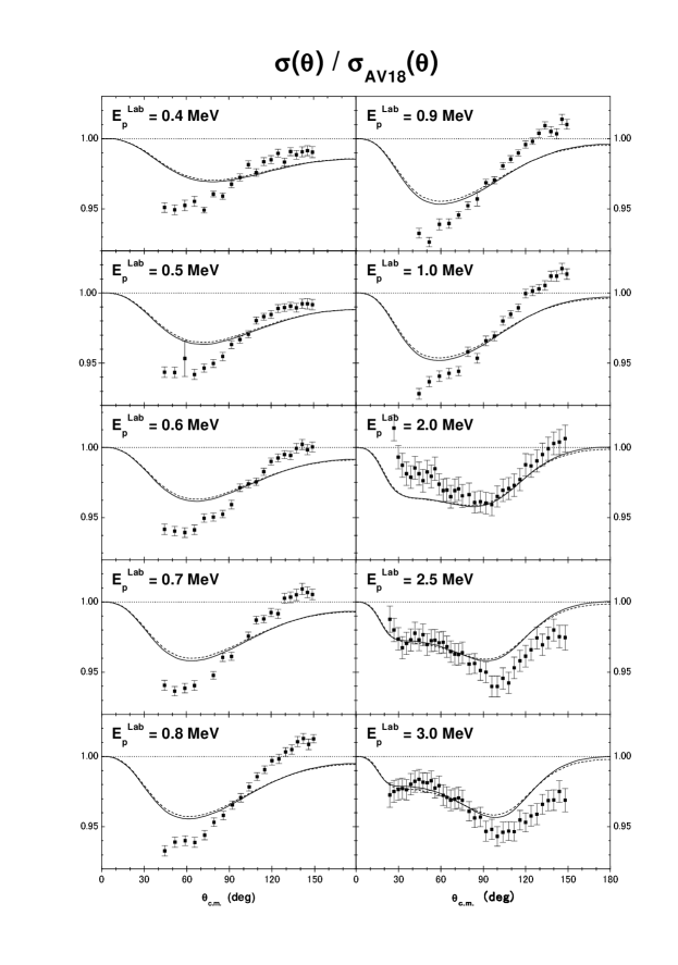
Figure 4: The $pd$ differential cross section normalized to those calculated with AV18. Solid curves are those with AV18+BR. Dashed curves are those with AV18+GS. Experimental data are taken from ref. [1] for $E_{p}^{\mathrm{Lab}}=0.4-1.0$ MeV, and from ref. [3] for $E_{p}^{\mathrm{Lab}}=2.0-3.0$ MeV.

3.4 Nucleon Vector Analyzing Powers

In Fig. 5, we show results of the proton analyzing power $A_{y}(\theta)$ at several energies below three-body breakup threshold comparing with available experimental data [1, 4]. The results with the AV18 potential (dashed curves) undershoot the experimental values of $A_{y}(\theta)$ (The $A_{y}$ puzzle). The inclusion of the BR-3NF into the nuclear Hamiltonian increases only a small amount of $A_{y}(\theta)$ as denoted by the solid curves. On the other hand, the phenomenological spin-orbit 3NF, LS1 [40], improves $A_{y}(\theta)$ considerably as denoted by dotted curves. It is noted that the small amount of overestimation in $A_{y}(\theta)$ with AV18+BR+LS1 above 2 MeV is because of the combination of the LS1-3NF with the BR-3NF since the spin-orbit 3NFs in ref. [40] are made so as to reproduce the experimental values of $A_{y}(\theta)$ by themselves,

A merit to accommodate the Coulomb interaction in 3N system is that we can discuss the effect of CSB with high quality by comparing calculations with and without the Coulomb interaction. In ref. [16], CSB effects are studied for 3N bound states. It was demonstrated that the calculated values of the $\mathrm{}^{3}H$ binding energy ($B(\mathrm{}^{3}H)$) and those of $\mathrm{}^{3}He$ ($B(\mathrm{}^{3}He)$) for various combinations of NN forces and 3NFs have a linear correlation. When we plot the results of $B(\mathrm{}^{3}He)$ without any CSB effect (but only with the Coulomb force) against those of $B(\mathrm{}^{3}H)$, these points are fitted by a line, which does not pass through the point of the experimental values. When we include a CSB NN force, which reproduces the experimental difference of the proton-proton and neutron-neutron ¹S₀ scattering lengths, $\Delta a$ = 1.5 fm, together with the higher order electromagnetic interaction, we can draw a line that shifts to pass the experimental point. The CSB force used in the study of the 3N bound states is a central one. On the other hand, information of non-central spin-dependent CSB forces is expected to be given from the study of polarization observables in the $nd$ and the $pd$ scatterings. So far, the nucleon vector analyzing power $A_{y}(\theta)$ was measured for the $nd$ and the $pd$ elastic scattering for some energies [4, 43, 44]. The measured values of $A_{y}(\theta)$ have peaks at $\theta_{c.m.}\sim 105^{\circ}$ at low energies. The difference between the $\polarize{n}d$ and $\polarize{p}d$ $A_{y}(\theta)$ peak heights, which depends weakly on incident energies below $E_{N}^{\mathrm{Lab}}=10$ MeV, and is roughly 0.01.

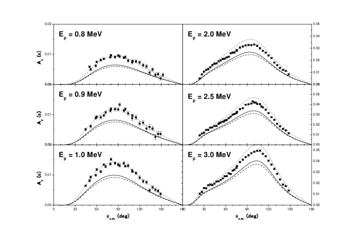
Figure 5: Analyzing powers of the incident proton in the $pd$ scattering at $E_{p}^{\mathrm{Lab}}=0.8-3.0$ MeV. Dashed curves are calculations with AV18, solid curves those with AV18+BR, and dotted curves those with AV18+BR+LS1. Experimental date are from ref. [1] for $E_{p}^{\mathrm{Lab}}$ = 0.8, 0.9, and 1.0 MeV, and from ref. [4] for $E_{p}^{\mathrm{Lab}}$ = 2.0, 2.5, and 3.0 MeV.

In Fig. 6, the calculated values of the difference, $A_{y}^{nd}-A_{y}^{pd}|_{\theta_{\mathrm{c.m.}}=105^{\circ}}$ at $E_{N}^{\mathrm{Lab}}$ = 3 MeV are plotted against their average values, $\left(A_{y}^{nd}+A_{y}^{pd}\right)/2|_{\theta_{\mathrm{c.m.}}=105^{\circ}}$. In this figure, the results with AV14^′ and AV14^′+BR+LS1 are plotted as open circles, those with dTRS^′ and dTRS^′+BR+LS1 as open triangles, and those with AV18, AV18+BR, and AV18+BR+3NF as open squares. Apparently, the results are divided into two groups that are linearly correlated: one is the results with AV14^′ or dTRS^′ NN potentials as guided by the dotted line, and the other is those with AV18 as guided by the dashed line.

We remark that the difference between these lines is attributed to higher order electromagnetic (EM) interactions in the AV18 potential. The EM interactions include a spin-orbit force arising from the magnetic moment interaction, which contributes as a CSB force [34]. To demonstrate the effect of the EM spin-orbit CSB interaction (EMls), a result of calculation with AV18 neglecting EMls is plotted as a filled square, and that with AV14^′ including EMls as a filled circle in Fig. 6. The former point almost lies on the dotted line, and the latter on the dashed one. We therefore conclude that the higher order electromagnetic interaction in the AV18 model explains the difference of the two lines in Fig. 6, and gives about 10% effect in the $nd$-$pd$ analyzing power difference.

In ref. [45], the effect of the EM spin-orbit force is reported to be small in $Nd$ analyzing power. However, the deuteron was treated as a single spin-1 particle in ref. [45]. The present result therefore shows an importance of a three-body treatment of the $pd$ system.

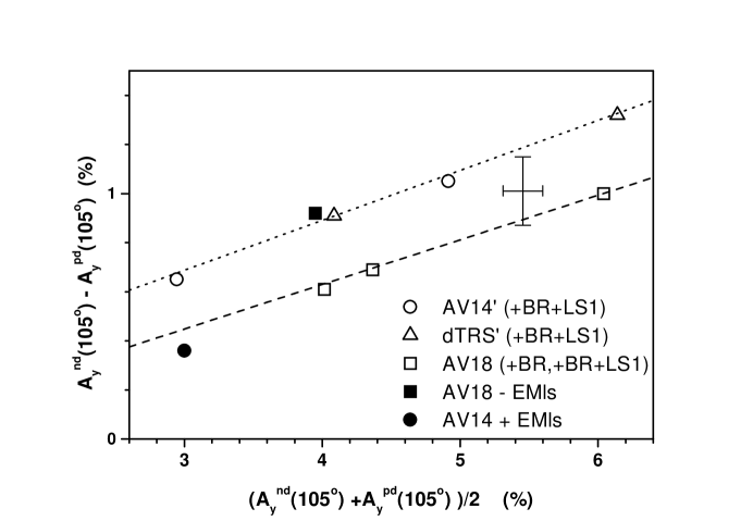
Figure 6: $A_{y}^{nd}-A_{y}^{pd}$ vs. $(A_{y}^{nd}+A_{y}^{pd})/2$ at $\theta_{\mathrm{c.m.}}=105^{\circ}$. Experimental date are taken from [4, 43]. The meaning of the points is described in the text.

4 Summary

We have formally derived a modified Faddeev equation to accommodate the long-range Coulomb interaction in three-nucleon ($pd$) scattering, which was originally presented in ref. [12]. In the modification, we introduced an auxiliary Coulomb force that acts between a spectator proton and the c.m. of the rest pair nucleons (proton and neutron). This interaction takes into account two issues: (1) the Coulomb distortion of the spectator particle and (2) the cancellation of the long-rang part of the original Coulomb force in the integral kernel for energies below the three-body breakup threshold. The modified Faddeev equation can be treated similarly as in the case of the $nd$ scattering.

We presented some numerical results to solve the Coulomb modified Faddeev equation for the $pd$ elastic scattering at energies below the three-body breakup threshold for some realistic NN potential models without or with three-nucleon forces. Results of the phase shift parameters agree with the available accurate results by different methods.

Differential cross sections for an NN potential overestimate the experimental data by about 5% at low energies. This overestimation is recovered by introducing three-nucleon forces that reproduce the 3N binding energy.

CSB effects are studied for the nucleon analyzing powers in $pd$ scattering and $nd$ scattering at 3 MeV. We found that a spin-orbit force due to the nucleon magnetic moment interaction plays a significant role in the difference.

This research was supported by the Japan Society for the Promotion of Science, under Grant-in-Aid for Scientific Research No. 13640300. The numerical calculations have been supported by the Computational Science Research Center, Hosei University, under project lab0003.

References

- [1] Huttel, E., et al.: Nucl. Phys. A406, 435 (1983)
- [2] Knutson, L. D., Lamm, L. O., McAninch, J. E.: Phys. Rev. Lett. 71, 3762 (1993)
- [3] Sagara, K., et al.: Phys. Rev. C 50, 576 (1994)
- [4] Shimizu, S., et al.: Phys. Rev. C 52, 1193 (1995)
- [5] Sakamoto, N., et al.: Phys. Lett. B 367, 60 (1996)
- [6] Bieber, R., et al.: Phys. Rev. Lett. 84, 606 (2000)
- [7] Sakai, H., et al.: Phys. Rev. Lett. 84, 5288 (2000)
- [8] Cadman, R. V., et al.: Phys. Rev. Lett. 86, 967 (2001)
- [9] Brune, C. R., et al.: Phys. Rev. C 63, 044013 (2001)
- [10] Ermisch, K., et al.: Phys. Rev. Lett. 86, 5862 (2001)
- [11] Wood, M. H., et al.: Phys. Rev. C 65, 034002 (2002)
- [12] Sasakawa, T., Sawada, T.: Phys. Rev. C 20, 1954 (1979)
- [13] Faddeev, L. D.: Zh. Eksp. Teor. Fiz. 39, 1459 (1960) [Sov. Phys.-JETP 12, 1041 (1961)]
- [14] Sasakawa, T., Okuno, H., Sawada, T.: Phys. Rev. C 23, 905 (1981)
- [15] Wu, Y., Ishikawa, S., Sasakawa, T.: Phys. Rev. Lett. 64, 1875 (1990); 66, 242 (1991)
- [16] Wu, Y., Ishikawa, S., Sasakawa, T.: Few-Body Syst. 15, 145 (1993)
- [17] Sasakawa, T., Ishikawa, S.: Few-Body Syst. 1, 3 (1986)
- [18] Ishikawa, S.: Nucl. Phys. A463, 145c (1987)
- [19] Alt, E. O., Sandhas, W., Ziegelmann, H.: Phys. Rev. C 17, 1981 (1978)
- [20] Berthold, G. H., Stadler, A., Zankel, H.: Phys. Rev. C 41, 1365 (1990)
- [21] Alt, E. O., Sandhas, W.: In: Coulomb Interactions in Nulcear and Atomic Few-Body Collisions (Levin, F. S., Micha, D. A., eds.): p. 1. New York and London: Plenum Press 1996
- [22] Alt, E.O., Mukhamedzhanov, A. M., Sattarov, A. I.: Phys. Rev. Lett. 81, 4820 (1998)
- [23] Chen, C. R., et al.: Phys. Rev. C 39, 1261 (1989)
- [24] Friar, J. L., Payne, G. L.: In: Coulomb Interactions in Nulcear and Atomic Few-Body Collisions (Levin, F. S., Micha, D. A., eds.): p. 97. New York and London: Plenum Press 1996
- [25] Chen, C. R., Friar, J. L., Payne, G. L.: Few-Body Syst. 31, 13 (2001)
- [26] Papp, Z.: Phys. Rev. C 55, 1080 (1997)
- [27] Kievsky, A., Viviani, M., Rosati, S.: Phys. Rev. C 52, R15 (1995)
- [28] Kievsky, A., et al.: Nucl Phys. A 607, 402 (1996)
- [29] Messiah, A.: Quantum Mechanics. New York: John Wiley 1965
- [30] Malfliet, R. A., Tjon, J. A.: Nucl. Phys. A127, 161 (1969)
- [31] Payne, G. L., et al.: Phys. Rev. C 32, 823 (1980)
- [32] Wiringa, R. B., Smith, R. A., Ainsworth, T. L.: Phys. Rev. C. 29, 1207 (1984)
- [33] Kievsky A., et al.: Phys. Rev. C 63, 064004 (2001)
- [34] Wiringa, R. B., Stoks, V. G. J., Schiavilla, R.: Phys. Rev. C 51, 38 (1995)
- [35] Hüber, D., et al..: Phys. Rev. C 51, 1100 (1995)
- [36] Coelho, H. T., Das, T. K., Robilotta, M. R.: Phys. Rev. C 28, 1812 (1983)
- [37] Koike, Y., Haidenbauer, J.: Nucl. Phys. A463, 365c (1987)
- [38] Witała, H., Glöckle, W., Cornelius, T.: Nucl. Phys. A491, 157 (1988)
- [39] Ishikawa, S.: Phys. Rev. C 59, R1247 (1999)
- [40] Kievsky, A.: Phys. Rev. C 60, 034001 (1999)
- [41] Doleschall, P., et al.: Nucl. Phys. A380, 72 (1982).
- [42] de Tourreil, R., Rouben, B., Sprung, D. W. L.: Nucl. Phys. 242, 445 (1975)
- [43] McAninch, J. E., Lamm, L. O., Haeberli, W.: Phys. Rev. C 50, 589 (1994)
- [44] Nishimori, N., et al.: Nucl. Phys. A 631, 697c (1998)
- [45] Stoks, V. G. J.: Phys. Rev. C 57, 445 (1998)