Quantum Monte Carlo calculations of $A=9,10$ nuclei

Abstract

We report on quantum Monte Carlo calculations of the ground and low-lying excited states of $A=9,10$ nuclei using realistic Hamiltonians containing the Argonne $v_{18}$ two-nucleon potential alone or with one of several three-nucleon potentials, including Urbana IX and three of the new Illinois models. The calculations begin with correlated many-body wave functions that have an $\alpha$-like core and multiple p-shell nucleons, $LS$-coupled to the appropriate $(J^{\pi};T)$ quantum numbers for the state of interest. After optimization, these variational trial functions are used as input to a Green’s function Monte Carlo calculation of the energy, using a constrained path algorithm. We find that the Hamiltonians that include Illinois three-nucleon potentials reproduce ten states in ⁹Li, ⁹Be, ¹⁰Be, and ¹⁰B with an rms deviation as little as 900 keV. In particular, we obtain the correct 3⁺ ground state for ¹⁰B, whereas the Argonne $v_{18}$ alone or with Urbana IX predicts a 1⁺ ground state. In addition, we calculate isovector and isotensor energy differences, electromagnetic moments, and one- and two-body density distributions.

I INTRODUCTION

In a series of papers PPCW95 ; PPCPW97 ; WPCP00 , we have reported quantum Monte Carlo (QMC) calculations of ground and low-lying excited state energies in $A\leq 8$ nuclei for realistic nuclear Hamiltonians. These calculations employed the Argonne $v_{18}$ (AV18) two-nucleon potential WSS95 and the Urbana IX (UIX) three-nucleon potential PPCW95 , and are accurate to $\approx 1-2\%$ of the binding energy for light p-shell nuclei. More recently, we have used the quantum Monte Carlo calculations to help construct a series of new and improved pion-exchange-based three-nucleon potentials, designated the Illinois models PPWC01 . The five Illinois models (IL1-IL5), when used in conjunction with AV18, each reproduce the experimental energies of 17 narrow states in $A\leq 8$ nuclei with an rms deviation of $\approx 400$ keV. This contrasts with a 2.3 MeV rms deviation for the AV18/UIX Hamiltonian, and 7.7 MeV for AV18 alone.

In this paper, we report the extension of our QMC calculations to $A=9,10$ nuclei. The QMC methods include both variational (VMC) and Green’s function Monte Carlo (GFMC) methods. The VMC method is used to construct a variational wave function as a product of two and three-body correlation operators acting on a independent-particle wave function that has an $\alpha$-like core and multiple p-shell nucleons, $LS$-coupled to the appropriate $(J^{\pi};T)$ quantum numbers for the state of interest. Monte Carlo evaluation of the energy expectation value is used to optimize the trial function, particularly the mix of independent-particle wave function components. The GFMC method starts from this trial function and makes a Euclidean propagation that converges to the lowest energy for a state of these quantum numbers. A constrained path algorithm is crucial for keeping the fermion sign problem under control. At present the GFMC method is used to calculate only the lowest state of given $(J^{\pi};T)$.

We have calculated ten stable or very narrow natural-parity states in the $A=9,10$ nuclei ⁹Li, ⁹Be, ¹⁰Be, and ¹⁰B that are experimentally well known. We use three of the new Illinois models (IL2, IL3, IL4) in conjunction with AV18 and obtain rms deviations from the experimental energies of the states of 900, 1100, and 1700 keV, respectively. We have also calculated most of these states with the AV18 and AV18/UIX Hamiltonians for comparison. The most intriguing result we find is that the new AV18/IL2-IL4 models all correctly predict a 3⁺ ground state for ¹⁰B, but the older models wrongly predict a 1⁺ ground state. In addition, we have made GFMC calculations of six other states that are expected within the p-shell formulation of these nuclei and of the ⁹He and ¹⁰He ground states; these states either have much larger widths or are not clearly identified by experiment.

We review briefly the experimental status of the ground and low-lying excited states in the $A=9,10$ nuclei in Sec. II. The Hamiltonians are described in Sec. III and the QMC calculations in Sec. IV. Most of this material has been discussed in detail in Refs. PPCPW97 ; WPCP00 . The only major new technical development is the automation of the construction of the independent-particle portion of the variational trial wave functions that serve as starting points for the GFMC calculations. Energy results are given in Sec. V, while electromagnetic moments and density distributions are shown in Sec. VI. We present our conclusions in Sec. VII.

II EXPERIMENTAL STATUS

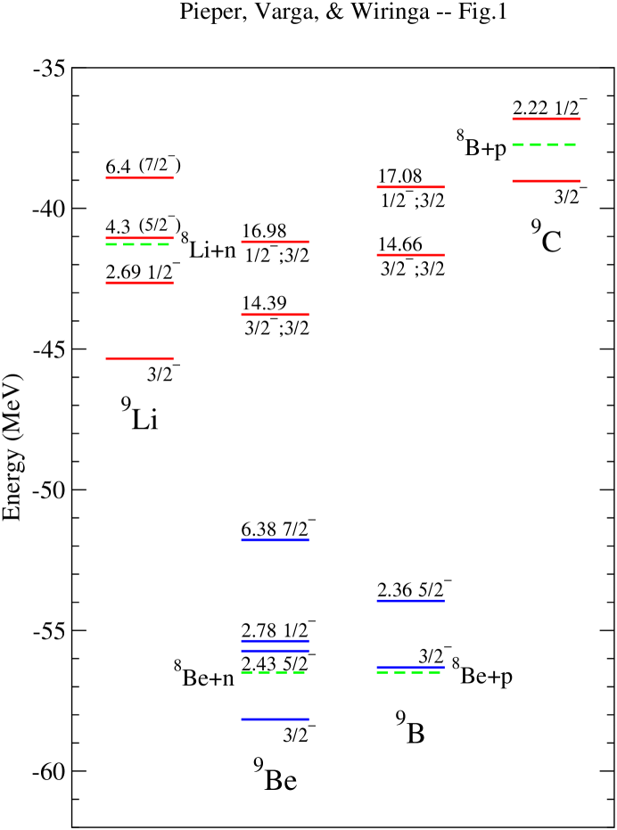
Figure 1: First natural-parity states in the experimental spectra of $A=9$ nuclei.

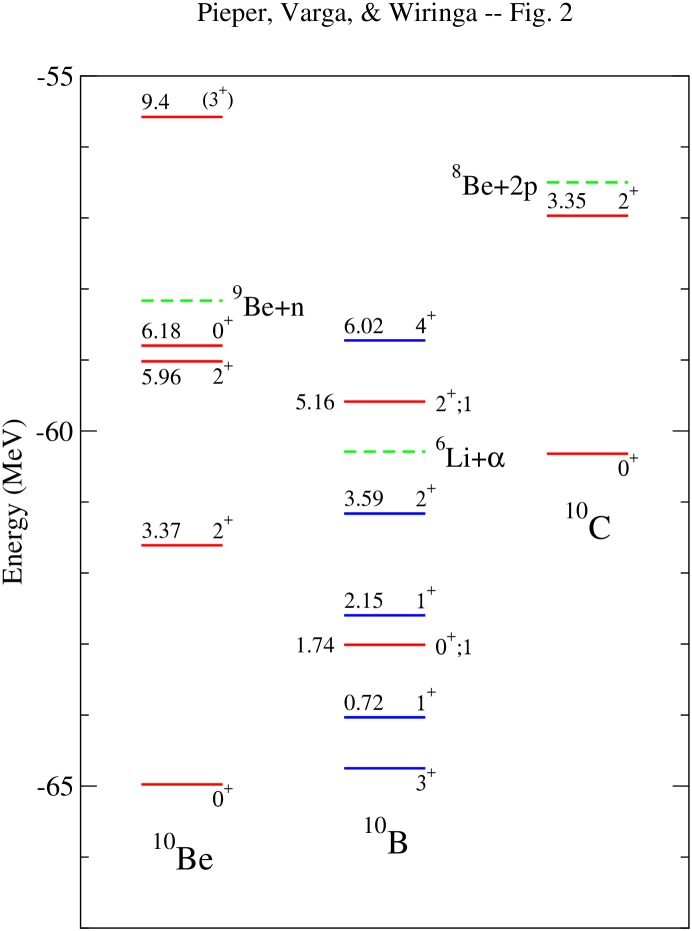
Figure 2: Low-lying natural-parity states in the experimental spectra of $A=10$ nuclei.

The experimental status of $A=9,10$ nuclei is illustrated in Figs. 1 and 2, where we show the ground states and most low-lying natural-parity states whose spin assignments are reasonably certain AS88 ; Til01 . We also show some additional narrow states in ⁹Li and ¹⁰Be whose spins have not been determined experimentally; reasonable guesses are given in parentheses, based on standard shell model studies and the present calculations.

The ground state of ⁹Be is an absolutely stable $(J^{\pi};T)=(\frac{3}{2}^{-};\frac{1}{2})$ state. The first excitation is a $(\frac{1}{2}^{+};\frac{1}{2})$ state (not shown in Fig. 1) with a width of 217 keV which occurs at the threshold for breakup into ${}^{8}{\rm Be}+n$. This unnatural parity state is beyond the scope of the present paper; we will report calculations of such intruder states in the future. The second excitation is a narrow $(\frac{5}{2}^{-};\frac{1}{2})$ state at 2.429 MeV, with a width $<1$ keV. Within the p-shell formulation, there can also be $(\frac{1}{2}^{-};\frac{1}{2})$, $(\frac{7}{2}^{-};\frac{1}{2})$, and $(\frac{9}{2}^{-};\frac{1}{2})$ states. Experimentally, the first two are observed at 2.78 and 6.38 MeV excitation but both are quite broad ($\approx 1$ MeV), while no state with $(\frac{9}{2}^{-};\frac{1}{2})$ character has been identified. We evaluate all these $(J^{\pi};T)$ cases in GFMC, treating the states as if they were particle stable; this should be adequate for narrow states, but may be less satisfactory for broad states. (Several additional unnatural parity states and second excited states of given $(J^{\pi};T)$ are observed above 3 MeV, but are not shown in the figure.) The matrix elements of the electromagnetic and strong charge-independence-breaking terms in the Hamiltonian are evaluated perturbatively to infer the energies of the narrow $T=\frac{1}{2}$ isobaric analog states in ⁹B.

The ground state of ⁹Li is a particle stable ($\frac{3}{2}^{-};\frac{3}{2}$) state that decays by $\beta^{-}$ emission to ⁹Be with a half-life of 178 ms. The first excited state of ⁹Li at 2.691 MeV is believed to be a ($\frac{1}{2}^{-};\frac{3}{2}$) state; it is below the threshold for breakup into ${}^{8}{\rm Li}+n$ and decays only by $\gamma$ emission. We calculate both these states in ⁹Li, and again perturbatively evaluate the energies of the isobaric analogs in ⁹Be, ⁹B, and ⁹C. Two additional narrow states above the breakup threshold have been observed in ⁹Li, but without firm spin-parity identification: a 60 keV wide state at 4.296 MeV and a 40 keV wide state at 6.43 MeV. Within the p-shell, these should be ($\frac{5}{2}^{-};\frac{3}{2}$) and ($\frac{7}{2}^{-};\frac{3}{2}$) states; our GFMC evaluations of such states line up very well with the experimental observations, suggesting these spin assignments may indeed be correct.

The ground state of ¹⁰B is an absolutely stable (3⁺;0) state. The first threshold for breakup of ¹⁰B is into ⁶Li+$\alpha$. Between the ground state and breakup threshold are two (1⁺;0) excited states at 0.718 MeV and 2.154 MeV, one (2⁺;0) state at 3.587 MeV, and the (0⁺;1) isobaric analog of ¹⁰Be at 1.740 MeV. Many additional states are known above the ⁶Li+$\alpha$ threshold; in Fig. 2 we show only the (2⁺;1) isobaric analog at 5.164 MeV and the (4⁺;0) state at 6.025 MeV. We calculate the (3⁺;0) ground state and first (1⁺;0), (2⁺;0), and (4⁺;0) excitations by GFMC. In the p-shell there can also be (0⁺;0) and (5⁺;0) states, but the former is of low spatial symmetry while the latter has high angular momentum, leading us to expect both of them to be quite high in excitation energy; no experimental observation of either has been made.

The nucleus ¹⁰Be is particle-stable but decays by $\beta^{-}$ emission with the very long half-life of $1.51\times 10^{6}$ years. As is typical for an even-even nucleus, the ground state is a (0⁺;1) state, and there is a well-separated (2⁺;1) excited state at 3.368 MeV. These are the two primary ¹⁰Be states we evaluate in GFMC. In addition, the tabulation lists a state at 9.4 MeV as a possible (2⁺;1) state, but a more recent (t,³He) experiment makes a (3⁺;1) assignment more likely 10Be3 ; Millener . We have made one computation for the (3⁺;1) level using AV18/IL2 and get reasonable agreement with this energy. Other particle-stable states below the threshold for breakup into ⁹Be+$n$ include second (0⁺;1) and (2⁺;1) states, also shown in Fig. 2, and the first particle-stable (1^-;1) and (2^-;1) intruder states (not shown). The second excited states are not evaluated at present in GFMC, while the intruder states will be reported on in future work. Again, the isobaric analog states in ¹⁰B and ¹⁰C are evaluated perturbatively from ¹⁰Be.

In addition to these nuclei, we have also made calculations of the expected lowest natural-parity states in ⁹He and ¹⁰He. These are a $(\frac{1}{2}^{-};\frac{5}{2})$ resonance which is observed at $\approx 1.2$ MeV above the threshold for breakup into ⁸He+$n$, and a $(0^{+};3)$ resonance at $\approx 1.1$ MeV above the ⁸He+$n$+$n$ threshold Til01 ; KPB99 . These resonances are observed to be reasonably narrow, with widths of 100 and $\leq 300$ keV, respectively. There are recent experimental reports of a $(\frac{1}{2}^{+};\frac{5}{2})$ resonance near threshold in ⁹He msu-expt , which we have not attempted to calculate; such a state is likely to be very broad and really needs to be treated as a scattering state. We also have not attempted to calculate the resonant ground state of ¹⁰Li, which is broad and still has some experimental uncertainty.

III HAMILTONIAN

The Hamiltonian includes nonrelativistic one-body kinetic energy, the AV18 two-nucleon potential WSS95 and either the UIX PPCW95 or one of the Illinois PPWC01 three-nucleon potentials:

$$H=\sum_{i}K_{i}+\sum_{i<j}v_{ij}+\sum_{i<j<k}V_{ijk}\ .$$ (1)

The kinetic energy operator is predominantly charge-independent (CI), but has a small charge-symmetry breaking (CSB) component due to the difference between proton and neutron masses. The AV18 is one of a class of highly accurate $N\!N$ potentials that fit both $pp$ and $np$ scattering data up to 350 MeV with a $\chi^{2}/$datum $\approx 1$. It can be written as a sum of electromagnetic and one-pion-exchange terms and a shorter-range phenomenological part:

$$v_{ij}=v^{\gamma}_{ij}+v^{\pi}_{ij}+v^{R}_{ij}\ .$$ (2)

The electromagnetic terms include one- and two-photon-exchange Coulomb interaction, vacuum polarization, Darwin-Foldy, and magnetic moment terms, all with appropriate proton and neutron form factors. The one-pion-exchange part of the potential includes the small charge-dependent (CD) terms due to the difference in neutral and charged pion masses. The shorter-range part has about 40 parameters which are adjusted to fit the $pp$ and $np$ scattering data, the deuteron binding energy, and also the $nn$ scattering length.

The one-pion-exchange and the remaining phenomenological part of the potential can be written as a sum of eighteen operators,

$$v^{\pi}_{ij}+v^{R}_{ij}=\sum_{p=1,18}v_{p}(r_{ij})O^{p}_{ij}\ .$$ (3)

The first fourteen CI operators are

$$O^{p=1,14}_{ij}=[1,{\bf\sigma}_{i}\cdot{\bf\sigma}_{j},S_{ij},{\bf L\cdot S},{\bf L}^{2},{\bf L}^{2}{\bf\sigma}_{i}\cdot{\bf\sigma}_{j},({\bf L\cdot S})^{2}]\otimes[1,{\bf\tau}_{i}\cdot{\bf\tau}_{j}]\ ,$$ (4)

while the last four,

$$O^{p=15,18}_{ij}=[1,{\bf\sigma}_{i}\cdot{\bf\sigma}_{j},S_{ij}]\otimes T_{ij},\ \tau_{zi}+\tau_{zj}\ ,$$ (5)

are the strong interaction CD and CSB terms.

The three-nucleon potentials from the Urbana series of models CPW83 contain a long-range, two-pion-exchange, P-wave term and a short-range phenomenological piece:

$$V^{U}_{ijk}=V^{2\pi,P}_{ijk}+V^{R}_{ijk}\ .$$ (6)

The UIX model has the strengths of these two terms adjusted to reproduce the binding energy of ³H, in GFMC calculations, and to give a reasonable saturation density in nuclear matter, in variational chain summation calculations AP97 , when used with AV18. The Illinois models add a two-pion-exchange S-wave term and a three-pion-ring term:

$$V^{IL}_{ijk}=V^{2\pi,P}_{ijk}+V^{2\pi,S}_{ijk}+V^{3\pi,\Delta R}_{ijk}+V^{R}_{ijk}\ .$$ (7)

The two-pion-exchange S-wave term is required by chiral symmetry, but in practice its small energy contribution makes it hard to distinguish from the dominant P-wave term. However, the three-pion-ring term, while it is smaller than the two-pion-exchange P-wave term, has a distinctly different isospin dependence, which is crucial for being able to fit the variety of light p-shell energy levels studied in Ref. PPWC01 . In the Illinois models, the operator structure and radial forms were taken from standard meson-exchange theory, but the overall strengths of the four terms, and one cutoff factor in the radial dependence, were adjusted to obtain best fits to the energies of 17 narrow states in $3\leq A\leq 8$ nuclei. In practice, at most three parameters at a time could be uniquely determined from the energy calculations, so five different models were constructed in which different subsets of the parameters were fixed by external considerations, while the remaining ones were adjusted.

The CD and CSB terms in $H$ are fairly weak, so we can treat them conveniently as a first-order perturbation and use a wave function of good isospin, which is significantly more compact. Also, direct GFMC calculations with the spin-dependent terms that involve the square of the orbital angular momentum operator can have large statistical fluctuations, as discussed in Ref. PPCPW97 . Thus it is useful to define PPCPW97 a simpler isoscalar interaction, AV8^′, which contains only the eight operators $[1,{\bf\sigma}_{i}\cdot{\bf\sigma}_{j},S_{ij},{\bf L\cdot S}]\otimes[1,{\bf\tau}_{i}\cdot{\bf\tau}_{j}]$ and an isoscalar Coulomb interaction. These eight operators are chosen such that AV8^′ reproduces the CI part of the full AV18 interaction in all S and P waves as well as the deuteron. The AV8^′ interaction (without the Coulomb term) was recently used in a benchmark test of seven different many-body methods for solving the four-nucleon bound state, with excellent agreement between GFMC and the other calculations KNG01 .

IV QUANTUM MONTE CARLO

IV.1 Variational Monte Carlo

We first construct a variational wave function for the state of interest and then optimize it by minimizing the energy expectation value as computed by Metropolis Monte Carlo integration. The variational wave function for the nuclei studied here has the form

$$|\Psi_{V}\rangle=\Big{[}1+\sum_{i<j<k}\tilde{U}^{TNI}_{ijk}\Big{]}{\cal S}\prod_{i<j}\Big{(}1+U_{ij}\Big{)}|\Psi_{J}\rangle\ .$$ (8)

The $U_{ij}$, and $\tilde{U}^{TNI}_{ij;k}$ are noncommuting two- and three-nucleon correlation operators, and ${\cal S}$ is a symmetrization operator. The $U_{ij}$ includes spin, isospin, and tensor terms induced by the two-nucleon potential, while the $\tilde{U}^{TNI}_{ij;k}$ reflects the structure of the dominant parts of the three-nucleon interaction. This trial function has the advantage of being efficient to evaluate while including the bulk of the correlation effects. A more sophisticated variational function can be constructed by including two-body spin-orbit correlations and additional three-body correlations, as discussed in Ref. WPCP00 , but the time to compute these extra terms is significant, while the gain in the variational energy is relatively small. Studies have shown that the GFMC algorithm easily corrects for the omission of these terms PPCPW97 .

The two-body correlations are generated by the solution of coupled differential equations with embedded variational parameters W91 . We have found that the parameters optimized for the $\alpha$-particle are near optimal for use in the light p-shell nuclei. Likewise, the best parameters for the three-body correlations are remarkably constant for different s- and p-shell nuclei, so they have not been changed significantly from the previous $A\leq 8$ work PPCPW97 ; WPCP00 .

For the p-shell nuclei studied here, the totally antisymmetric Jastrow wave function, $\Psi_{J}$, starts with a sum over independent-particle terms, $\Phi_{A}$, that have 4 nucleons in an $\alpha$-like core and $(A-4)$ nucleons in p-shell orbitals. We use $LS$ coupling to obtain the desired $JM$ value of a given state, as suggested by standard shell-model studies CK65 . We also need to specify the spatial symmetry $[n]$ of the angular momentum coupling of the p-shell nucleons BM69 . Different possible $LS[n]$ combinations lead to multiple components in the Jastrow wave function. This independent-particle basis is acted on by products of central pair and triplet correlation functions, which depend upon the shells (s or p) occupied by the particles and on the $LS[n]$ coupling:

$$|\Psi_{J}\rangle = {\cal A}\left.\Big{\{}\right.\prod_{i<j<k\leq 4}f^{c}_{ijk}\prod_{i<j\leq 4}f_{ss}(r_{ij})\prod_{k\leq 4<l\leq A}f_{sp}(r_{kl})$$ (9)

$$\sum_{LS[n]}\Big{(}\beta_{LS[n]}\prod_{4<l<m\leq A}f^{[n]}_{pp}(r_{lm})\ |\Phi_{A}(LS[n]JMTT_{3})_{1234:5\ldots A}\rangle\Big{)}\left.\right.\Big{\}}\ .$$

The operator ${\cal A}$ indicates an antisymmetric sum over all possible partitions of the $A$ particles into 4 s-shell and $(A-4)$ p-shell ones. The pair correlation for particles within the s-shell, $f_{ss}(r)$, is the optimal correlation for the $\alpha$-particle. The $f_{sp}(r)$ is similar to the $f_{ss}(r)$ at short range, but with a long-range tail going to a constant $\approx 1$; this allows the wave function to develop a cluster structure like $\alpha+d$ in ⁶Li or $\alpha+\alpha$ in ⁸Be at large cluster separations. The $f^{[n]}_{pp}(r)$ depends on the nucleus and particular independent-particle channel, e.g., in the case of ⁶Li or ⁸Be, it is similar to the optimal deuteron or alpha correlations.

The $LS[n]$ components of the independent-particle wave function are given by:

$$|\Phi_{A}(LS[n]JMTT_{3})_{1234:5\ldots A}\rangle=|\Phi_{\alpha}(0000)_{1234}\prod_{4<l\leq A}\phi^{LS[n]}_{p}(R_{\alpha l})$$

$$\left\{[\prod_{4<l\leq A}Y_{1m_{l}}(\Omega_{\alpha l})]_{LM_{L}[n]}\otimes[\prod_{4<l\leq A}\chi_{l}(\frac{1}{2}m_{s})]_{SM_{S}}\right\}_{JM}\otimes[\prod_{4<l\leq A}\nu_{l}(\frac{1}{2}t_{3})]_{TT_{3}}\rangle\ ,$$ (10)

where

$$\Phi_{\alpha}(0000)={\cal A}(p\uparrow p\downarrow n\uparrow n\downarrow)$$ (11)

is the $\alpha$-core independent-particle wave function. The $\phi^{LS}_{p}(R_{\alpha l})$ are $p$-wave solutions of a particle of reduced mass $\frac{4}{5}m_{n}$ in an effective $\alpha$-$N$ potential:

$$V_{\alpha N}(r)=V^{WS}_{\alpha N}(r)+V^{C}_{\alpha N}(r)\ .$$ (12)

The $\phi^{LS}_{p}$ are functions of the distance between the center of mass of the $\alpha$ core (which contains particles 1-4 in this partition) and nucleon $l$, and again may be different for different $LS[n]$ components. For each state considered in the present work, we have used bound-state asymptotic conditions for the $\phi^{LS}_{p}$, even if the state is particle unstable. The Woods-Saxon potential

$$V^{WS}_{\alpha N}(r)=V^{LS}_{p}[1+{\rm exp}(\frac{r-R_{p}}{a_{p}})]^{-1}\ ,$$ (13)

has variational parameters $V^{LS}_{p}$, $R_{p}$, and $a_{p}$, while the Coulomb potential is obtained by folding over nuclear and nucleon form factors. The wave function is translationally invariant, hence there is no spurious center of mass motion.

A major technical advance in the present work is the automatic generation of the independent-particle wave function $\Phi_{A}$ with the appropriate spatial symmetries discussed above. We describe here the construction of the spatial symmetry $[n]$. One can use different coupling schemes to form the spatial (or spin and isospin) part of the wave function with good quantum numbers. We use simple sequential coupling in which the spatial part of the wave function is written as

$$\theta_{LM_{L}\mu}=\left[\left[\left[Y_{1}({\Omega_{\alpha 5}})Y_{1}({\Omega_{\alpha 6}})\right]_{l_{56}}Y_{1}({\Omega_{\alpha 7}})\right]_{l_{567}}....\right]_{LM_{L}},$$ (14)

and a similar construction is used for the spin and isospin part. The functions having the same $L$ and $M_{L}$ but different intermediate quantum numbers, labeled by $\mu$, are orthogonal and form a complete set of eigenstates of $L^{2}$ and $L_{z}$. The permutation operators $P_{k}$ of the valence particles $l=5,6,...,A$ ($k=1,...,(A-4)!$), commute with $L^{2}$ and $L_{z}$ so that the above functions form a basis for the representation of the symmetric group as well:

$$P_{k}\theta_{LM_{L}\mu}=\sum_{\lambda}U_{\lambda\mu}(P_{k})\theta_{LM_{L}\lambda}\ .$$ (15)

The permutation symmetry is conveniently depicted by using “Young diagrams”, consisting of $N$ adjoining square boxes with rows numbered numerically downward, and columns rightward; there may not be more rows in column $i$ than in column $i-1$, nor columns in row $j$ than in row $j-1$. Each Young diagram corresponds to a representation of the permutation group. The basis functions defining a given representation can be labeled by using a Young tableau, which is an arrangement of the numbers $1,2,...,N$ in the Young diagram, such that numbers always increase along all rows and down all columns.

We use the “Young operators” to construct a basis function that has the symmetry properties of a given Young tableau. The Young operator, ${\hat{Y}}$, is a product of a symmetrizer $R$ and an antisymmetrizer $Q$: ${\hat{Y}}=QR$. The operator $R$ symmetrizes all particle indices which are in the same row and $Q$ antisymmetrizes all particles in the same column. Both operators are constructed as a combination of the permutation operators $P_{k}$.

To construct the spatial part of the wave function belonging to a given representation of the permutation group, we first have to draw the Young diagram and insert the numbers $1,2,...,N$ into the pattern in any order to give a Young tableau. The number of different tableaux $N_{Y}$ is the dimension of the representation. Then we prepare the Young operators ${\hat{Y}}_{1},...,{\hat{Y}}_{N_{Y}}$ corresponding to the Young tableau and calculate the matrix elements of these operators with the basis functions $\theta_{LM_{L}\mu}$. We then have

$${\hat{Y}}_{k}\theta_{LM_{L}\mu}=\sum_{\lambda}\langle\theta_{LM_{L}\mu}|{\hat{Y}}_{k}|\theta_{LM_{L}\lambda}\rangle\theta_{LM_{L}\lambda}.$$ (16)

Let us denote the successively coupled spin (isospin) functions by $\omega_{SM_{S}nu}$ ($\omega_{TT_{3}\nu^{\prime}}$). To form an antisymmetric wave function for the $N$ particle system one has to multiply the basis functions of the space part of a given Young tableau, ${\hat{Y}}_{k}\theta_{LM_{L}\mu}$, by the basis functions of the spin-isospin part belonging to the conjugated $[{\bar{n}}]$ Young diagram (obtained by reversal of the roles of rows and columns) ${\hat{Y}}_{k}[{\bar{n}}]\omega_{SM_{S}\nu}\omega_{TT_{3}\nu^{\prime}}$ and sum over all possible tableaux. Thus, Eq.(10) becomes:

$$|\Phi_{A}(LS[n]JMTT_{3})_{1234:5\ldots A}\rangle = |\Phi_{\alpha}(0000)_{1234}\prod_{4<l\leq A}\phi^{LS[n]}_{p}(R_{\alpha l})$$ (17)

$$\sum_{k}p_{k}{\hat{Y}}_{k}[n]{\hat{Y}}_{k}[{\bar{n}}]\left[\theta_{L\mu}\omega_{S\nu}\right]_{JM}\omega_{TT_{3}\nu^{\prime}}\rangle\ ,$$

where $p_{k}$ is the parity of the permutation of the numbers (starting from the top and going left to right in each row) in the Young diagram. The Young operator ${\hat{Y}}_{k}[n]$ (${\hat{Y}}_{k}[{\bar{n}}]$) acts on the spatial (spin-isospin) functions of the $l=5,6,...,A$ valence particles. Any choice of $\mu$ and $\nu,\nu^{\prime}$ generates the same wave function.

The different possible $LS[n]$ contributions to $A=9,10$ nuclei are given in Table 1. After other parameters in the trial function have been optimized, a series of energy evaluations are made in which the $\beta_{LS[n]}$ of Eq.(9) are different in the left- and right-hand-side wave functions to obtain the diagonal and off-diagonal matrix elements of the Hamiltonian and the corresponding normalizations and overlaps. The resulting N$\times$N matrices are diagonalized to find the $\beta_{LS[n]}$ eigenvectors, using generalized eigenvalue routines because the correlated $\Psi_{V}$ are not orthogonal. This allows us to project out not only the ground-state trial functions, but also excited-state trial functions of the same $(J^{\pi};T)$ quantum numbers. In our present studies, we have carried out our $A$=9 diagonalization in a complete p-shell basis, but for ¹⁰B and ¹⁰Be we have limited ourselves to the three highest spatial symmetries, i.e., [42], [33], and [411]. The diagonalization is carried out for the AV18/UIX Hamiltonian; the $\beta_{LS[n]}$ amplitudes should not be significantly different for the other models. Additional spatial symmetries involving particle excitations out of the p-shell are built up in the full trial function by means of the tensor correlations contained in the $U_{ij}$ and $\tilde{U}^{TNI}_{ijk}$ of Eq.(8).

Thus in ⁹Be, the Jastrow wave function for the $(\frac{3}{2}^{-};\frac{1}{2})$ ground state is constructed from thirteen amplitudes, and a $13\times 13$ diagonalization is performed to find the optimal mixing. The $\beta_{LS[n]}$ values for this and other ⁹Be states, including some second excited states, are given in Table 2, while the values for various states in ⁹Li are given in Table 3. In the case of ⁹Be, the [41] symmetry states dominate; addition of the lower spatial symmetries improves the energies by typically 0.25 MeV. The additional states do not significantly alter the rms radii or electromagnetic moments. By contrast, the leading [32] symmetry in ⁹Li is not so dominant; addition of lower spatial symmetries gives a significant 1–2 MeV improvement to some of the energies. Electromagnetic moments can also be significantly shifted. In general, the dominant $A=9$ amplitudes are in good agreement (modulo sign) with the shell-model wave functions of Kumar K74 .

The $\beta_{LS[n]}$ values for ¹⁰B states are given in Table 4, and for ¹⁰Be states in Table 5. The neglect of the [321] or lower symmetry states in these nuclei is justified on the grounds that this is the leading spatial symmetry of ¹⁰Li, whose isobaric analog state first appears at 21 MeV in the excitation spectrum of ¹⁰Be. For ¹⁰B, the [42] symmetry states are dominant, and addition of the [33] and [411] symmetries improves the energies by only 0.2 MeV. However, for ¹⁰Be, these extra components can give significant additional binding of up to 3 MeV. In this case, the extra states correspond to low-lying excitations that may not be filtered out of the trial function by a GFMC propagation to limited $\tau$, as discussed below. Thus it is crucial to carry out the diagonalization in the trial function to get an optimal starting point for the GFMC calculation.

The $A=10$ nuclei are exactly midway through the p-shell and are unique in having two linearly independent states of the same spatial symmetry contribute, i.e., two ¹D[42] states in ¹⁰Be and two ³D[42] states in ¹⁰B. To uniquely identify these two possible combinations, we diagonalize Jastrow trial functions containing just the two ^2S+1D[42] states in the quadrupole moment operator, so the first $\beta_{LS[n]}$ amplitude reported in Tables 4–5 for each state corresponds to the lower (negative) quadrupole eigenvalue and the second to the higher (positive) quadrupole eigenvalue. Interestingly, we see that most states where these two symmetries contribute are dominated by either one amplitude or the other, e.g., the first 3⁺ in ¹⁰B is almost pure positive quadrupole while the second 3⁺ is almost pure negative quadrupole in composition. Similarly the first 2⁺ in ¹⁰Be is almost pure negative quadrupole while the second is pure positive quadrupole. This is analogous to using the $LK_{L}$ labeling scheme applied to ¹⁰B by Kurath in a traditional shell model calculation K79 , and there is good agreement as to the dominant [42] symmetry amplitudes with his Table 3. Only the first 2⁺ state in ¹⁰B does not seem to fit in with these observations.

Energy expectation values with the full $\Psi_{V}$ of Eq.(8) are evaluated by a Metropolis Monte Carlo algorithm as described in PPCPW97 . The full wave function at any given spatial configuration ${\bf R}={\bf r}_{1},{\bf r}_{2},...{\bf r}_{A}$ can be represented by a vector of $2^{A}\times I(A,T)$ complex numbers,

$$\Psi({\bf R})=\sum_{\alpha}\psi_{\alpha}({\bf R})|\alpha\rangle\ ,$$ (18)

where the $\psi_{\alpha}({\bf R})$ are the complex coefficients of each state $|\alpha\rangle$ which has specific third components of spin and linear combinations of good isospin. For the nuclei considered here, this leads to vectors ranging in length from 13,824 for ⁹He to 92,160 for ¹⁰Be, although a savings of a factor of two is possible in even-$A$ nuclei by computing in the $M=0$ substates. The spin, isospin, and tensor operators $O^{p=2,6}_{ij}$ contained in the potential and other operators of interest are sparse matrices in this basis and thus easily evaluated. Kinetic energy and spin-orbit operators require the computation of first derivatives and diagonal second derivatives of the wave function. These are obtained by evaluating the wave function at $6A$ slightly shifted positions of the coordinates ${\bf R}$ and taking finite differences. Terms quadratic in ${\bf L}$ require mixed second derivatives and additional wave-function evaluations and finite differences.

IV.2 Green’s Function Monte Carlo

The GFMC method C87 ; C88 projects out the exact lowest-energy state, $\Psi_{0}$, for a given set of quantum numbers, using $\Psi_{0}=\lim_{\tau\rightarrow\infty}\exp[-(H-E_{0})\tau]\Psi_{T}$, where $\Psi_{T}$ is an optimized trial function from the VMC calculation. If the maximum $\tau$ actually used is large enough, the eigenvalue $E_{0}$ is calculated exactly while other expectation values are generally calculated neglecting terms of order $|\Psi_{0}-\Psi_{T}|^{2}$ and higher PPCPW97 . In contrast, the error in the variational energy is of order $|\Psi_{0}-\Psi_{T}|^{2}$, and other expectation values calculated with $\Psi_{T}$ have errors of order $|\Psi_{0}-\Psi_{T}|$. In the following we present a brief overview of the nuclear GFMC method; much more detail may be found in Refs. PPCPW97 ; WPCP00 .

We start with a $\Psi_{T}$ defined as (see Eq.(3.13) of Ref. WPCP00 )

$$|\Psi_{T}\rangle={\cal S}\prod_{i<j}\Big{(}1+U_{ij}+\sum_{k\neq i,j}\tilde{U}^{TNI}_{ij;k}\Big{)}|\Psi_{J}\rangle\ ,$$ (19)

and define the propagated wave function $\Psi(\tau)$

$$\Psi(\tau)=e^{-({H}-E_{0})\tau}\Psi_{T}=\left[e^{-({H}-E_{0})\triangle\tau}\right]^{n}\Psi_{T}\ ,$$ (20)

where we have introduced a small time step, $\triangle\tau=\tau/n$; obviously $\Psi(\tau=0)=\Psi_{T}$ and $\Psi(\tau\rightarrow\infty)=\Psi_{0}$. The $\Psi(\tau)$ is represented by a vector function of $\bf R$ using Eq.(18), and the Green’s function, $G_{\alpha\beta}({\bf R},{\bf R}^{\prime})$ is a matrix function of $\bf R$ and ${\bf R}^{\prime}$ in spin-isospin space, defined as

$$G_{\alpha\beta}({\bf R},{\bf R}^{\prime})=\langle{\bf R},\alpha|e^{-({H}-E_{0})\triangle\tau}|{\bf R}^{\prime},\beta\rangle\ .$$ (21)

It is calculated with leading errors of order $(\triangle\tau)^{3}$. Omitting the spin-isospin indices $\alpha$, $\beta$ for brevity, $\Psi({\bf R}_{n},\tau)$ is given by

$$\Psi({\bf R}_{n},\tau)=\int G({\bf R}_{n},{\bf R}_{n-1})\cdots G({\bf R}_{1},{\bf R}_{0})\Psi_{T}({\bf R}_{0})d{\bf R}_{n-1}\cdots d{\bf R}_{1}d{\bf R}_{0}\ ,$$ (22)

with the integral being evaluated stochastically. The short-time propagator is constructed with the exact two-body propagator and additional terms coming from the three-body interaction.

Quantities of interest are evaluated in terms of a “mixed” expectation value between $\Psi_{T}$ and $\Psi(\tau)$:

$$\langle O\rangle_{\rm Mixed} = \frac{\langle\Psi_{T}|O|\Psi(\tau)\rangle}{\langle\Psi_{T}|\Psi(\tau)\rangle}$$ (23)

$$= \frac{\int d{\bf P}_{n}\Psi_{T}^{\dagger}({\bf R}_{n})OG({\bf R}_{n},{\bf R}_{n-1})\cdots G({\bf R}_{1},{\bf R}_{0})\Psi_{T}({\bf R}_{0})}{\int d{\bf P}_{n}\Psi_{T}^{\dagger}({\bf R}_{n})G({\bf R}_{n},{\bf R}_{n-1})\cdots G({\bf R}_{1},{\bf R}_{0})\Psi_{T}({\bf R}_{0})}~{},$$

where ${\bf P}_{n}={\bf R}_{0},{\bf R}_{1},\cdots,{\bf R}_{n}$ denotes the ‘path’, and $d{\bf P}_{n}=d{\bf R}_{0}d{\bf R}_{1}\cdots d{\bf R}_{n}$ with the integral over the paths being carried out stochastically. The desired expectation values would, of course, have $\Psi(\tau)$ on both sides; by writing $\Psi(\tau)=\Psi_{T}+\delta\Psi(\tau)$ and neglecting terms of order $[\delta\Psi(\tau)]^{2}$, we obtain the approximate expression

$$\langle O(\tau)\rangle=\frac{\langle\Psi(\tau)|O|\Psi(\tau)\rangle}{\langle\Psi(\tau)|\Psi(\tau)\rangle}\approx\langle O(\tau)\rangle_{\rm Mixed}+[\langle O(\tau)\rangle_{\rm Mixed}-\langle O\rangle_{T}]~{},$$ (24)

where $\langle O\rangle_{T}$ is the variational expectation value.

A special case is the expectation value of the Hamiltonian. The $\langle{H}(\tau)\rangle_{\rm Mixed}$ can be re-expressed as

$$\langle{H}(\tau)\rangle_{\rm Mixed}=\frac{\langle\Psi_{T}|e^{-({H}-E_{0})\tau/2}{H}e^{-({H}-E_{0})\tau/2}|\Psi_{T}\rangle}{\langle\Psi_{T}|e^{-({H}-E_{0})\tau/2}e^{-({H}-E_{0})\tau/2}|\Psi_{T}\rangle}\geq E_{0}~{},$$ (25)

since the propagator $\exp[-(H-E_{0})\tau]$ commutes with the Hamiltonian. Thus $\langle{H}(\tau)\rangle_{\rm Mixed}$ approaches $E_{0}$ in the limit $\tau\rightarrow\infty$, and the expectation value obeys the variational principle for all $\tau$.

As mentioned above, the propagation is actually made with a simplified Hamiltonian $H^{\prime}$ that includes the CI kinetic energy operator, the AV8^′ two-nucleon interaction including isoscalar Coulomb, and a slightly altered $V^{\prime}_{ijk}$ three-nucleon interaction. The AV8^′ is a little more attractive than AV18, so a slightly more repulsive $V^{\prime}_{ijk}$ is used to keep $\langle H^{\prime}\rangle\approx\langle H\rangle$. This ensures the GFMC algorithm will not propagate to excessively large densities due to overbinding. Consequently, the upper bound property applies to $\langle{H}^{\prime}(\tau)\rangle$, and $\langle H-H^{\prime}\rangle$ must be evaluated perturbatively.

Another complication that arises in the GFMC algorithm is the “fermion sign problem”. This arises from the stochastic evaluation of the matrix elements in Eq.(23). The Monte Carlo techniques used to calculate the path integrals leading to $\Psi({\bf R}_{n},\tau)$ involve only local properties, while antisymmetry is a global property. Thus the propagation can mix in the boson solution. This has a (much) lower energy than the fermion solution and thus is exponentially amplified in subsequent propagations. In the final integration with the antisymmetric $\Psi_{T}$, the desired fermionic part is projected out, but in the presence of large statistical errors that grow exponentially with $\tau$. Because the number of pairs that can be exchanged grows with $A$, the sign problem also grows exponentially with increasing $A$. For $A{\geq}8$, the errors grow so fast that convergence in $\tau$ cannot be achieved.

To remedy this situation, a “constrained path” approximation has been developed WPCP00 . The basic idea of the constrained-path method is to discard those configurations that, in future generations, will contribute only noise to expectation values. Many tests of the constrained path have been made and it usually gives results that are consistent with unconstrained propagation, within statistical errors, although there are cases in which it converges to the wrong energy WPCP00 . Up to now, this problem was always solved by using a small number, $n_{u}=10$ to 20, of unconstrained steps before evaluating expectation values. These few unconstrained steps, out of 400 or more total steps, were enough to damp out errors introduced by the constraint in all the tests that we had done. The statistical errors in calculations with $n_{u}=10$ are not substantially greater than for $n_{u}=0$. However for $A=10$, the error from $n_{u}=20$ is 60–90% larger than that from $n_{u}=10$, i.e., 2.5–3.5 more configurations must be used to get the same error. In the present work, we find that $A=9,10$ calculations with the AV18/IL3 Hamiltonian (which has the strongest long-range part of $V_{ijk}$) are particularly sensitive to $n_{u}$, and most of these are made with $n_{u}=20$. Tests made with the other Hamiltonians show that $n_{u}=10$ is enough, except for ^9,10He.

Previously WPCP00 we had found that obtaining reliable results for ⁸He was particularly difficult. In the present work we find that this persists for ^9,10He which show large statistical fluctuations. In addition the constrained-path method appears to be less reliable than for other nuclei. For example, we made a calculation for ¹⁰He with AV18/IL2 and a $\Psi_{T}$ that contained no $N\!N\!N$ correlation. Even though $n_{u}=20$ was used, the result was overbound by 1.5(6) MeV. (In Ref. WPCP00 a calculation of ⁶Li with a much worse $\Psi_{T}$, which contained no $NN$ tensor correlations, also gave an overbound result but this was corrected with only $n_{u}=10$.) The statistical errors using $n_{u}=40$ are very large, making a confirmation of the $n_{u}=20$ results presented here difficult; we have attempted this for AV18/IL2 and obtain no significant change in the binding energy within a statistical error of 0.7 MeV.

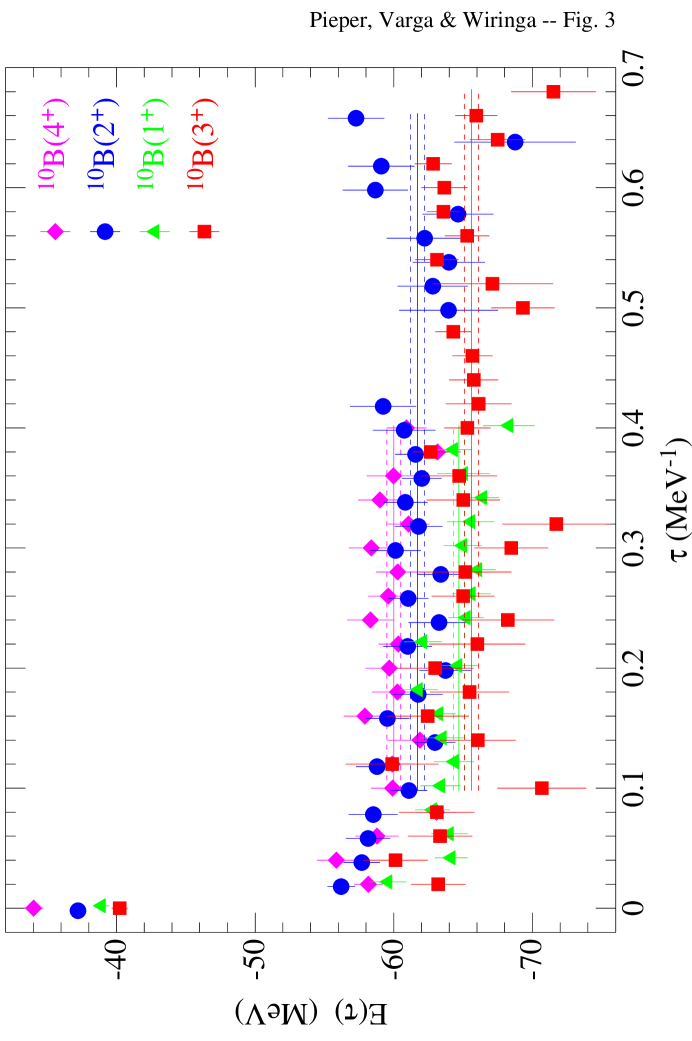
Figure 3: GFMC $E(\tau)$ for states of ¹⁰B calculated for the AV18/IL2 Hamiltonian. The solid lines show the averages that are reported in the text; the dashed lines show the corresponding statistical errors.

Figure 3 shows the progress with increasing $\tau$ of typical constrained GFMC calculations, in this case for various states of ¹⁰B using the AV18/IL2 Hamiltonian. The values shown at $\tau=0$ are the VMC values using $\Psi_{T}$. The GFMC very rapidly makes a large improvement on these energies; by $\tau=0.01$ MeV^-1, the $\Psi_{T}$ energies have been reduced by $\sim$20 MeV. This rapid improvement corresponds to the removal of small admixtures of states with excitation energies $\sim 1$ GeV from $\Psi_{T}$. Typically, averages over the $\tau\geq 0.1$ MeV^-1 values are used as the GFMC energy. The standard deviation, computed using block averaging, of all of the individual energies for these $\tau$ values is used to compute the corresponding statistical error. The solid lines show these averages; the corresponding dashed lines show the statistical errors.

V ENERGY RESULTS

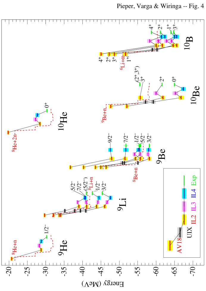
Figure 4: GFMC and experimental energies for $A=9,10$ nuclei. The light shading shows the Monte Carlo statistical errors or experimental widths.

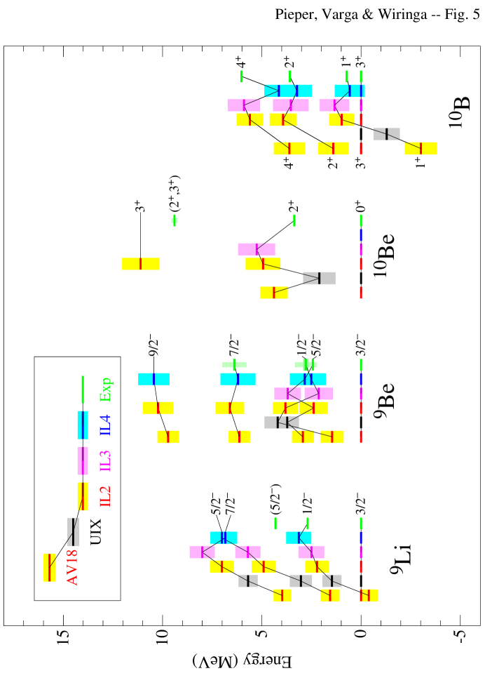
Figure 5: GFMC and experimental excitation energies for $A=9,10$ nuclei.

In this section we present GFMC energy results in $A=9,10$ nuclei for the simplified AV8^′ $N\!N$ Hamiltonian, the full AV18 interaction, and AV18 with each of the $N\!N\!N$ interactions UIX, IL2, IL3, and IL4. (Results for $A\leq 8$ nuclei may be found in Ref. PPWC01 .) The total energies for 18 states are shown in Table 6 and in Fig. 4; excitation spectra are shown in Fig. 5. Not all states have been calculated with all the Hamiltonians. Numbers in parentheses are the Monte Carlo statistical errors; in addition there may be systematic errors from the GFMC algorithm of the order of 1–2% percent as discussed above.

The energies of the particle-stable ground states calculated with just the $N\!N$ interactions are underbound by 8–12 MeV in $A=9$ and 12–16 MeV in $A=10$, with the AV8^′ being somewhat more attractive than AV18. Addition of the older UIX $N\!N\!N$ interaction to AV18 reduces this discrepancy significantly to 2–4 MeV in $A=9$ and 4–6 MeV in $A=10$. However, addition of the IL2-IL4 models to AV18 results in much better energies, some high and some low, but generally within 2 MeV. In particular, the AV18/IL2 and AV18/IL3 Hamiltonians come within $\pm 3\%$ of the experimental bindings for the ground states of ⁹Li, ⁹Be, ¹⁰Be, and ¹⁰B, which is about as good as can be expected, given the 1–2% total errors in the GFMC calculation.

Despite their systematic underbinding, the older Hamiltonians were able to give the correct ordering of excited states in the $A\leq 8$ nuclei, albeit usually with insufficient splitting between states that are spin-orbit partners PPWC01 . In the $A=9,10$ nuclei this no longer holds true. The most dramatic case is the question of the proper ground state for ¹⁰B: AV8^′, AV18, and AV18/UIX all clearly and wrongly predict the $(1^{+};0)$ state to be lower than the $(3^{+};0)$ state, while all the AV18/IL2-IL4 models correctly reproduce the experimental ordering. This result for the AV18 interaction was first obtained by Navrátil who also finds it for the CD-Bonn interaction navratil . This incorrect ordering of states by the two-body Hamiltonians also seems to be present in the case of the $(\frac{5}{2}^{-};\frac{1}{2})$ and $(\frac{1}{2}^{-};\frac{1}{2})$ excitations of ⁹Be, and may be a problem for the proper ground state of ⁹Li, although with the statistical errors of the calculation it is not so clear. The AV18/UIX and AV18/IL2-IL4 models obtain these states in the proper order, with one exception, and generally with fairly good spin-orbit splittings.

As noted in Sec. II, two narrow, particle-unstable states have been observed in ⁹Li without definite spin assignments. On the basis of the close agreement between the AV18/IL2 energies for the lowest $(\frac{5}{2}^{-};\frac{1}{2})$ and $(\frac{7}{2}^{-};\frac{1}{2})$ states and the observed excitations, as illustrated in Fig. 5, we think these are in fact the most likely assignments for these states. Also, our one calculation of the expected $(3^{+};1)$ state in ¹⁰Be lines up with the observed state at 9.4 MeV, suggesting that is its proper spin assignment.

The current calculations significantly underbind ^9,10He, even when the AV18/IL2-IL4 models are used. Because both these nuclei are particle unstable, they should properly be calculated as resonant states, so the current GFMC results may be somewhat less reliable than for the other ground states. However, the experimental widths of these states are not large, and our calculations for other comparably narrow states have generally been good. It may be that some significant admixture of $1s_{1/2}$ orbitals from the sd-shell should be introduced in the Jastrow trial function, as suggested by recent shell-model studies OFUBHM01 ; we have not yet attempted such a modification. In addition, as was discussed in the previous section, the constrained-path propagation may not be as reliable for these nuclei. If the present results for ^9,10He are correct, then there is a need for further tuning of the isospin dependence of the $N\!N\!N$ interactions.

In addition to the total energies discussed above, we have calculated the energy differences between isobaric analog states perturbatively by evaluating the expectation values of the electromagnetic and strong CSB and CD parts of the AV18 Hamiltonian in the wave function of the $T_{z}=-T$ nucleus. The CSB and CD terms can induce corresponding changes in the nuclear wave functions, leading to higher-order perturbative corrections to the splitting of isospin mass multiplets, but it is difficult for us to estimate these higher-order effects reliably in either VMC or GFMC calculations. The energies for a given isomultiplet of states can be expanded as

$$E_{A,T}(T_{z})=\sum_{n\leq 2T}a_{n}(A,T)Q_{n}(T,T_{z})\ ,$$ (26)

where $Q_{0}=1$, $Q_{1}=T_{z}$, and $Q_{2}=\frac{1}{2}(3T_{z}^{2}-T^{2})$ are isoscalar, isovector, and isotensor terms P60 . The isovector coefficients $a_{1}(A,T)$ are shown in Table 7, while the isotensor coefficients $a_{2}(A,T)$, are given in Table 8.

The dominant contribution in each case is from the regular Coulomb interaction between protons, but there are additional contributions of $\approx 5\%$ coming from the other electromagnetic and strong terms. Because the AV18 and AV18/UIX models underbind these nuclei, the density distributions tend to be more diffuse and the Coulomb interaction is reduced, leaving a sizable discrepancy with experiment for the isovector coefficients. The AV18/IL2-IL4 models give much better binding energies and consequently larger isovector coefficients which are within 5% of the experimental values. However, the isotensor coefficients come out a bit too large.

VI MOMENTS AND DENSITY DISTRIBUTIONS

Point proton and neutron rms radii are shown in Tables 9 and 10. The AV18/IL2-IL4 Hamiltonians give significantly smaller radii than the older models, presumably because of their greater binding. The experimentally measured charge radii rms-expt for the ⁹Be and ¹⁰B ground states are in good agreement with the calculations from the new models.

Quadrupole moments are shown in Table 11, as evaluated in impulse approximation. Experimental values are from Refs. AS88 ; Til01 . The contribution of two-body charge operators to the quadrupole moment are expected to be small, as in the deuteron and ⁶Li WSS95 ; WS98 , because both the isoscalar and isovector charge operators are relativistic corrections of order $(v/c)^{2}$. Expectation values of the quadrupole operator tend to have a much larger variance than radii because of the cancellations from the $Y_{20}$ operator. Given this caveat, the agreement with the measured quadrupole moments is reasonable.

The impulse approximation magnetic moments are shown in Table 12; experimental values are from Refs. AS88 ; Til01 ; 9CMM ; 9CMMb . Experience in lighter nuclei shows that there are significant two-body current contributions to the magnetic operators, particularly the isovector part. In the trinucleons, the isoscalar portion is boosted by $+0.034\mu_{N}$ or $\approx 8\%$, while the isovector portion is corrected by $-0.778\mu_{N}$ or $\approx 18\%$ MRS98 . However, in the isoscalar ⁶Li case, the correction is a tiny +0.003 $\mu_{N}$ WS98 . On this basis, we expect substantial improvement in the ⁹Li and ⁹C results shown in Table 12 when two-body contributions to the current operator are added, while the already good ¹⁰B results will not be significantly affected. However, the reasonable agreement between the IA calculations and experiment for ⁹Be may not survive.

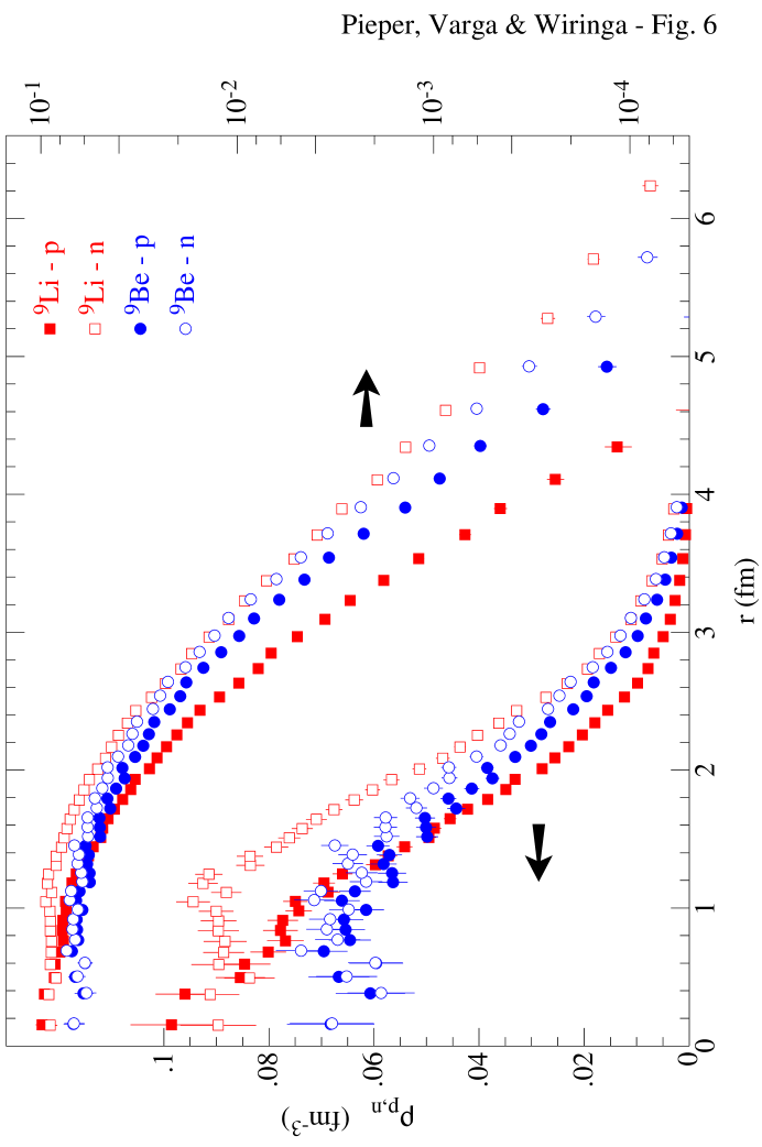
Figure 6: Proton and neutron densities for $A=9$ nuclei on both linear (left) and logarithmic (right) scales.

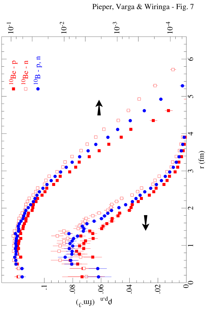
Figure 7: Proton and neutron densities for $A=10$ nuclei on both linear (left) and logarithmic (right) scales.

The nucleon densities for ⁹Li and ⁹Be are shown in Fig. 6, on both a linear (left) and logarithmic (right) scale. The densities are normalized such that the integrated value equals the appropriate total value of $N$ or $Z$. These densities are rather similar to those calculated earlier for ⁸Li and ⁸Be WPCP00 with the former more peaked at the origin, and the latter showing a broad flat interior. The protons in ⁹Li cluster at the origin because two out of three are confined to the $\alpha$ core, while the neutrons show a substantial skin with a hint of a p-shell peak around 1 fm. The low central densities for both protons and neutrons in ⁹Be are probably due to the large $2\alpha$ component in its ⁸Be core. The densities for ¹⁰Be and ¹⁰B are shown in Fig. 7. They have somewhat higher central values than in ⁹Be, but are also broader and flatter than ⁹Li, presumably due to the dominant ⁸Be core.

VII CONCLUSIONS

We have made quantum Monte Carlo calculations for the ground states and low-lying excited states of $A=9,10$ nuclei, based on realistic two- and three-nucleon potentials. The new Illinois $N\!N\!N$ models do a good job of explaining the binding energies of the ten best-known $A=9,10$ states of different quantum numbers, but the results for ^9,10He may indicate a deficiency in the models. If we also include the 17 narrow states to which these forces were fit in $A\leq 8$ nuclei PPWC01 , we find rms deviations from the experimental energies of 0.6 MeV for AV18/IL2, 0.8 MeV for AV18/IL3, and 1.0 MeV for AV18/IL4. This contrasts with rms deviations of 3.2 MeV for AV18/UIX and 9.9 MeV for AV18 alone. Thus AV18/IL2 becomes our preferred model Hamiltonian with AV18/IL3 almost as good, although AV18/IL4 will be somewhat deprecated.

We conclude that a fairly consistent picture of nuclear binding can be constructed for $A\leq 10$ nuclei using a single Hamiltonian and a single computational framework. This applies also to the energy differences among isobaric multiplets, which are well-reproduced. Electromagnetic moments, within the limitation of the impulse approximation, are in fairly good agreement with experimental data.

Significant challenges for the future will be the computation of second or higher excited states of the same quantum number, and intruder states of unnatural parity; both of these types of states first become particle-stable in the $A=10$ nuclei. We also need to evaluate electroweak transition rates in these nuclei, as has been done previously in the $A=6,7$ systems WS98 ; SW02 . The present calculations are at the limit of our current computer resources, both in CPU time and resident memory. However, the present codes are in principle capable of computing nuclei like ¹¹Be and ¹²C; such calculations may become feasible with the next generation of computers.

Table 1: Permutation symmetry terms for $LS$-coupling in $A=9,10$ nuclei and corresponding spin states.

$A$	$[n]$	$L$	$(T,S)$	highest symmetry states
$9$	$[41]$	$1,2,3,4$	$(\frac{1}{2},\frac{1}{2})$	9Be$(\frac{1}{2}^{-}$– $\frac{9}{2}^{-})$
	$[32]$	$1,2,3$	$(\frac{3}{2},\frac{1}{2})(\frac{1}{2},\frac{3}{2})(\frac{1}{2},\frac{1}{2})$	9Li$(\frac{1}{2}^{-}$– $\frac{7}{2}^{-})$
	$[311]$	$0,2$	$(\frac{3}{2},\frac{3}{2})(\frac{3}{2},\frac{1}{2})(\frac{1}{2},\frac{3}{2})(\frac{1}{2},\frac{1}{2})$
	$[221]$	$1$	$(\frac{5}{2},\frac{1}{2})(\frac{3}{2},\frac{3}{2})(\frac{3}{2},\frac{1}{2})(\frac{1}{2},\frac{5}{2})(\frac{1}{2},\frac{3}{2})(\frac{1}{2},\frac{1}{2})$	9He$(\frac{1}{2}^{-},\frac{3}{2}^{-})$
$10$	$[42]$	$0,2^{2},3,4$	$(1,0)(0,1)$	10Be$(0^{+},2^{+}$– $4^{+})$, 10B$(1^{+}$– $5^{+})$
	$[33]$	$1,3$	$(1,1)(0,0)$	10Be$(1^{+})$
	$[411]$	$1,3$	$(1,1)(0,0)$
	$[321]$	$1,2$	$(2,1)(2,0)(1,2)(1,1)^{2}(1,0)(0,2)(0,1)$	10Li$(0^{+}$– $3^{+})$, 10B$(0^{+})$
	$[222]$	$0$	$(3,0)(2,1)(1,2)(1,0)(0,3)(0,1)$	10He$(0^{+})$

Table 2: VMC diagonalization for $\beta_{LS[n]}$ components in ⁹Be.

$J^{\pi}$	2P[41]	2D[41]	2F[41]	2G[41]	4P[32]	4D[32]	4F[32]	2P[32]	2D[32]	2F[32]
$\frac{3}{2}^{-}$	0.936	–0.337			0.035	–0.024	0.047	–0.026	0.049
$\frac{5}{2}^{-}$		0.952	0.273		–0.064	–0.040	0.060		0.062	–0.041
$\frac{1}{2}^{-}$	0.990				0.117	–0.039		0.002
$\frac{7}{2}^{-}$			0.868	0.488		0.019	–0.064			0.034
$\frac{3}{2}^{-}$*	0.356	0.921			0.087	–0.098	0.052	–0.050	–0.003
$\frac{5}{2}^{-}$*		–0.248	0.925		0.273	0.007	0.045		0.037	–0.051
$\frac{9}{2}^{-}$				0.978			0.207
$\frac{1}{2}^{-}$*	–0.104				0.905	0.286		–0.153
$\frac{7}{2}^{-}$*			–0.474	0.836		–0.260	0.009			0.042
$J^{\pi}$	4S[311]	4D[311]	2S[311]	2D[311]	6P[221]	4P[221]	2P[221]
$\frac{3}{2}^{-}$	0.046	–0.025		0.011	0.029	–0.010	0.010
$\frac{5}{2}^{-}$		0.053		–0.005	–0.025	–0.015
$\frac{1}{2}^{-}$		–0.054	–0.023			–0.038	0.024
$\frac{7}{2}^{-}$		0.057			–0.015
$\frac{3}{2}^{-}$*	0.046	0.035		-0.000	–0.005	0.000	0.010
$\frac{5}{2}^{-}$*		0.003		–0.035	–0.017	0.021
$\frac{9}{2}^{-}$
$\frac{1}{2}^{-}$*		–0.112	0.216			–0.077	0.005
$\frac{7}{2}^{-}$*		–0.080			–0.015

Table 3: VMC diagonalization for $\beta_{LS[n]}$ components in ⁹Li.

$J^{\pi}$	2P[32]	2D[32]	2F[32]	4S[311]	4D[311]	2S[311]	2D[311]	4P[221]	2P[221]
$\frac{3}{2}^{-}$	0.859	–0.089		–0.446	–0.070		–0.198	0.107	–0.004
$\frac{1}{2}^{-}$	0.841				–0.487	0.219		0.028	0.085
$\frac{5}{2}^{-}$		0.968	–0.234		–0.045		–0.060	–0.042
$\frac{3}{2}^{-}$*	–0.130	0.844		–0.489	0.016		0.160	–0.017	–0.075
$\frac{7}{2}^{-}$			0.826		–0.563
$\frac{1}{2}^{-}$*	–0.029				0.333	0.934		–0.109	0.054
$\frac{5}{2}^{-}$*		–0.088	–0.518		0.821		0.163	–0.154

Table 4: VMC diagonalization for $\beta_{LS[n]}$ components in ¹⁰B.

$J^{\pi}$	3S[42]	3D[42]	3D[42]	3F[42]	3G[42]	1P[33]	1F[33]	1P[411]	1F[411]
$3^{+}$		0.036	0.995	–0.086	0.001		0.016		0.003
$1^{+}$	0.889	–0.225	0.368			0.068		–0.137
$1^{+}$*	0.179	0.922	0.024			–0.021		–0.342
$2^{+}$		0.467	0.884	0.023
$3^{+}$*		0.917	0.368	0.016	–0.047		0.021		0.142
$1^{+}$**	–0.042	–0.014	0.998			–0.025		–0.038
$2^{+}$*		–0.141	0.978	–0.154
$4^{+}$				0.901	0.433

Table 5: VMC diagonalization for $\beta_{LS[n]}$ components in ¹⁰Be.

$J^{\pi}$	1S[42]	1D[42]	1D[42]	1F[42]	1G[42]	3P[33]	3F[33]	3P[411]	3F[411]
$0^{+}$	0.812					0.109		0.573
$2^{+}$		0.944	–0.071			–0.050	0.005	0.288	–0.138
$2^{+}$*		–0.035	0.998			–0.030	0.019	0.032	0.017
$0^{+}$*	–0.462					–0.492		0.738
$3^{+}$				0.969			0.102		–0.225
$4^{+}$					0.867		–0.228		–0.443

Table 6: Total GFMC energies in MeV.

	AV8′	AV18	UIX	IL2	IL3	IL4	Expt
9He($\frac{1}{2}^{-}$)	$-$22.5(2)	$-$20.7(3)		$-$28.7(3)	$-$28.2(5)	$-$28.8(4)	$-$30.21(8)
9Li($\frac{3}{2}^{-}$)	$-$36.6(2)	$-$33.7(3)	$-$40.9(3)	$-$46.0(4)	$-$46.7(5)	$-$47.6(4)	$-$45.34
9Li($\frac{1}{2}^{-}$)	$-$36.8(2)	$-$34.0(3)	$-$39.4(3)	$-$43.8(4)	$-$44.2(4)	$-$44.5(5)	$-$42.65
9Li($\frac{5}{2}^{-}$)	$-$35.0(2)	$-$32.1(3)	$-$37.9(4)	$-$41.1(4)	$-$41.0(4)	$-$40.6(4)	$-$39.96(?)
9Li($\frac{7}{2}^{-}$)	$-$32.0(2)	$-$29.7(3)	$-$35.2(3)	$-$39.0(4)	$-$38.7(4)	$-$40.8(4)	$-$38.91(?)
9Be($\frac{3}{2}^{-}$)	$-$49.9(2)	$-$46.4(4)	$-$55.1(3)	$-$58.2(5)	$-$57.8(5)	$-$58.0(6)	$-$58.16
9Be($\frac{5}{2}^{-}$)	$-$47.8(2)	$-$43.5(3)	$-$51.3(5)	$-$55.8(5)	$-$54.1(4)	$-$55.1(5)	$-$55.73
9Be($\frac{1}{2}^{-}$)	$-$48.2(2)	$-$45.0(4)	$-$50.9(6)	$-$54.3(4)	$-$55.7(5)	$-$55.5(4)	$-$55.36
9Be($\frac{7}{2}^{-}$)	$-$43.5(2)	$-$40.3(3)		$-$51.5(5)		$-$51.8(7)	$-$51.78
9Be($\frac{9}{2}^{-}$)	$-$40.1(2)	$-$36.7(3)		$-$47.9(6)		$-$47.5(5)
10He(0+)	$-$21.2(2)	$-$19.8(3)		$-$28.4(3)	$-$27.2(6)	$-$27.7(5)	$-$30.34
10Be(0+)	$-$56.1(2)	$-$52.0(5)	$-$59.2(6)	$-$66.8(7)	$-$65.2(7)	$-$67.4(6)	$-$64.98
10Be(2+)	$-$51.9(2)	$-$47.7(5)	$-$57.1(6)	$-$61.8(5)	$-$59.9(6)	$-$61.1(6)	$-$61.61
10Be(3+)				$-$55.7(6)			$-$55.58
10B(3+)	$-$53.2(3)	$-$48.6(6)	$-$59.0(4)	$-$65.6(5)	$-$64.1(5)	$-$65.6(6)	$-$64.75
10B(1+)	$-$55.7(3)	$-$51.6(6)	$-$60.3(5)	$-$64.7(4)	$-$62.8(5)	$-$65.1(5)	$-$64.03
10B(2+)	$-$52.2(2)	$-$47.2(5)		$-$61.7(5)	$-$60.6(7)	$-$62.4(5)	$-$61.16
10B(4+)	$-$50.0(3)	$-$45.0(5)		$-$60.0(5)	$-$58.2(6)	$-$61.5(4)	$-$58.72

Table 7: Isovector energies in keV.

	AV18	UIX	IL2	IL3	IL4	EXPT
9Li($\frac{3}{2}^{-}$)	1900(8)	1860(7)	2000(7)	2041(7)	2113(7)	2104
9Li($\frac{1}{2}^{-}$)	1831(8)	1804(8)	2003(7)	1891(7)	2047(8)	1946
9Be($\frac{3}{2}^{-}$)	1751(10)	1738(9)	1857(10)	1833(10)	1878(14)	1851
9Be($\frac{5}{2}^{-}$)	1700(10)	1704(8)	1753(12)	1754(12)	1869(13)	1783
10Be(0+)	1970(10)	2115(12)	2235(12)	2140(13)	2307(11)	2329
10Be(2+)	2111(11)	1970(12)	2189(12)	2124(11)	2079(11)	2322

Table 8: Isotensor energies in keV.

	AV18	UIX	IL2	IL3	IL4	EXPT
9Li($\frac{3}{2}^{-}$)	182(9)	182(9)	197(8)	202(11)	204(9)	176
9Li($\frac{1}{2}^{-}$)	172(7)	181(8)	193(8)	181(8)	184(10)	160
10Be(0+)	257(25)	205(33)	250(24)	284(29)	314(27)	241
10Be(2+)	223(27)	196(35)	216(18)	183(23)	208(28)	199

Table 9: Proton rms radii in fm.

	AV8′	UIX	IL2	IL3	IL4	EXPT
9Li($\frac{3}{2}^{-}$)	2.19(1)	2.20(1)	2.04(1)	2.02(1)	1.94(1)
9Li($\frac{1}{2}^{-}$)	2.27(1)	2.23(1)	2.11(1)	2.29(1)	2.07(1)
9Be($\frac{3}{2}^{-}$)	2.41(1)	2.41(1)	2.38(1)	2.36(1)	2.33(1)	2.40(1)
9Be($\frac{5}{2}^{-}$)	2.41(1)	2.41(1)	2.38(1)	2.46(1)	2.27(1)
10Be(0+)	2.38(1)	2.30(1)	2.21(1)	2.32(1)	2.19(1)
10Be(2+)	2.33(1)	2.42(1)	2.26(1)	2.29(1)	2.28(1)
10B(3+)	2.40(1)	2.49(1)	2.33(1)	2.38(1)	2.27(1)	2.33(12)
10B(1+)	2.45(1)	2.48(1)	2.49(1)	2.52(1)	2.42(1)
10B(2+)	2.46(1)		2.38(1)	2.59(1)	2.29(1)
10B(4+)	2.42(1)		2.30(0)	2.41(1)	2.15(0)

Table 10: Neutron rms radii in fm.

	AV18	UIX	IL2	IL3	IL4
9Li($\frac{3}{2}^{-}$)	2.72(1)	2.76(1)	2.57(1)	2.52(1)	2.39(1)
9Li($\frac{1}{2}^{-}$)	2.84(1)	2.80(1)	2.56(1)	2.76(1)	2.53(1)
9Be($\frac{3}{2}^{-}$)	2.63(1)	2.63(1)	2.55(1)	2.56(1)	2.52(1)
9Be($\frac{5}{2}^{-}$)	2.67(1)	2.65(1)	2.62(1)	2.65(1)	2.48(1)
10Be(0+)	2.76(1)	2.56(1)	2.47(1)	2.59(1)	2.45(1)
10Be(2+)	2.66(1)	2.78(1)	2.55(1)	2.60(1)	2.62(1)
10B(3+)	2.40(1)	2.49(1)	2.33(1)	2.38(1)	2.27(1)
10B(1+)	2.45(1)	2.48(1)	2.49(1)	2.52(1)	2.42(1)
10B(2+)	2.46(1)		2.38(1)	2.59(1)	2.29(1)
10B(4+)	2.42(1)		2.30(0)	2.41(1)	2.15(0)

Table 11: Quadrupole moments in fm².

	AV8′	UIX	IL2	IL3	IL4	EXPT
9Li($\frac{3}{2}^{-}$)	$-$3.1(1)	$-$2.9(1)	$-$2.7(1)	$-$2.7(1)	$-$2.5(1)	$-$2.7(1)
9Be($\frac{3}{2}^{-}$)	5.0(3)	7.4(2)	8.5(3)	5.7(2)	6.8(3)	5.9(1)
9Be($\frac{5}{2}^{-}$)	$-$2.3(2)	$-$2.6(2)	$-$2.9(2)	$-$4.8(2)	$-$4.1(2)
9C($\frac{3}{2}^{-}$)	$-$3.7(3)	$-$5.5(3)	$-$5.1(3)	$-$4.4(3)	$-$5.3(3)
10Be(2+)	$-$10.1(3)	$-$8.0(4)	$-$5.0(4)	$-$9.6(4)	7.2(2)
10B(3+)	8.7(2)	12.0(2)	9.5(2)	9.4(2)	8.8(2)	8.5(1)
10B(1+)	1.2(1)	3.2(2)	3.1(1)	3.2(1)	2.1(1)
10B(2+)	$-$1.9(2)		$-$0.6(2)	$-$1.8(3)	$-$1.8(2)
10B(4+)	3.9(3)		3.8(2)	5.4(4)	3.8(2)

Table 12: Magnetic moments in $\mu_{N}$.

	AV8′	UIX	IL2	IL3	IL4	EXPT
9Li($\frac{3}{2}^{-}$)	2.91(1)	2.54(2)	2.47(2)	2.54(2)	2.54(2)	3.44(0)
9Li($\frac{1}{2}^{-}$)	$-$0.23(2)	$-$0.19(3)	$-$0.29(2)	$-$0.25(3)	$-$0.24(3)
9Be($\frac{3}{2}^{-}$)	$-$1.35(2)	$-$1.11(1)	$-$1.14(2)	$-$1.03(2)	$-$1.17(3)	$-$1.18(0)
9Be($\frac{5}{2}^{-}$)	$-$0.95(1)	$-$0.96(1)	$-$0.88(1)	$-$0.84(1)	$-$0.85(1)
9C($\frac{3}{2}^{-}$)	$-$1.08(3)	$-$0.71(5)	$-$0.63(4)	$-$0.72(4)	$-$0.70(4)	$-$1.39(0)
10B(3+)	1.82(1)		1.80(1)		1.80(1)	1.80(0)
10B(1+)	0.75(1)	0.78(1)	0.74(1)		0.77(1)	0.63(12)