Fragmentation of Nuclei at Intermediate and High Energies in Modified Cascade Model

Abstract

The process of nuclear multifragmentation has been implemented, together with evaporation and fission channels of the disintegration of excited remnants in nucleus-nucleus collisions using percolation theory and the intranuclear cascade model. Colliding nuclei are treated as face–centered–cubic lattices with nucleons occupying the nodes of the lattice. The site–bond percolation model is used. The code can be applied for calculation of the fragmentation of nuclei in spallation and multifragmentation reactions.

1 Introduction

The intranuclear cascade model is one of the basic tools for analyzing spallation and multifragmentation processes in nuclear collisions. In the traditional cascade model of hadron-nucleus and nucleus-nucleus interactions, particle production is treated in two stages. In the first fast stage, intranuclear cascade occurs inside the target and (or) the projectile nuclei and some nucleons from the target and projectile nuclei are knocked out, together with mesons. In the second stage, residual nuclei (generally, in an excited state) divide into two remnants in the fission channel or evaporate protons, neutrons and/or light nuclei, including helium isotopes. However, experimental data indicate that, at intermediate energies, a third competing process, multifragmentation, comes into play, in which excited remnants break up into intermediate mass fragments (IMF). There are two approaches for theoretical description of multifragmentation: dynamical and statistical. In statistical multifragmentation models, an excited remnant achieves thermal equilibrium state and then expands, eventually reaching the freeze–out volume. At this point it fragments into neutrons, light charged particles and IMFs. In dynamical models IMFs are formed at the fast stage of nuclear collision via dynamical forces between nucleons during the evolution of the total system of interacting projectile and target. In this case the whole system and its parts (projectile and target remnants) never pass through states of thermal equilibrium.

There is one more approach for description of the process of multifragmentation: percolation theory. Percolation models treat the nucleus as a lattice with nucleons located at nodes of the lattice. It has been found that results of percolation calculations depend significantly upon the details of the lattice structure. For reasons of computational convenience, the simple cubic lattice has been most frequently used in multifragmentation simulations[1], but several studies have found [2, 3] that the face-centered-cubic lattice more accurately reproduces the experimental distributions of fragment masses and their energy spectra.

Although lattice simulations have been found to reproduce multifragmentation data surprisingly well, there has been little examination of the role of the lattice arrangement of nucleons inside nuclei. That is, lattices were employed more as computational techniques, rather than as formal nuclear models. The appearance of solid state models of nuclear structure can be dated from the paper of Pauling in 1965 [4, 5, 6]. The most attractive lattice model is the face–centered–cubic (FCC) model proposed by Cook and Dallacasa[6] because it brings together shell, liquid-drop and cluster characteristics, as found in the conventional models, within a single theoretical framework. Unique among the lattice models, the FCC reproduces the entire sequence of allowed nucleon states as found in the shell model.

In the present paper we further develop the modified intranuclear cascade–evaporation code, (MCAS) elaborated by one of the authors [7], with the aim of inclusion of multifragmentation channels. The word ”modified” relates to the implementation of the concept of ”formation time” into traditional cascade calculations, as described in Section 3. The goodness of fit of the MCAS to experimental data has been reported in previous papers [7, 8] concerning multiparticle production in nucleus-nucleus collisions at intermediate and moderately high energies (up to 10–20 GeV/n). Since traditional cascade models consider nuclear structure as a dilute fermi gas, we reconstructed the model in the framework of the lattice nuclear model. For this purpose we implemented the FCC lattice arrangement of nucleons for the colliding nuclei according to the algorithm proposed in reference [9] (Section 2). Calculations of multifragmentation channels are performed on the basis of the bond-site model of percolation theory (Section 4). Comparisons with experimental data are given in Section 5.

2 FCC lattice model of nuclear structure

The FCC packing of nucleons, with protons and neutrons occupying lattice sites in alternating layers, can be seen as consisting of four interpenetrating cubes. A nearest-neighbor distance of about 2.0262 fm reproduces the known core density of nuclei (0.17 nucleons/fm³). The essence of the geometry of the FCC model can be shown using the quantum numbers that are assigned to each nucleon in the conventional shell model [9]. It is known that a nucleon’s distance from the center of the nucleus determines its principal quantum number n. The distance of the nucleon from the ”nuclear spin axis” determines its total angular momentum (quantum number j). Finally, the distance of each nucleon from the $y-z$ plane determines its magnetic quantum number m. The inherent simplicity of the FCC model is evident in the FCC definitions of the eigenvalues:

$${\bf n} = (\left|x\right|+\left|y\right|+\left|z\right|-3)/2,$$ (1)

$${\bf j} = (\left|x\right|+\left|y\right|-1)/2,$$ (2)

$$\left|{\bf m}\right| = \left|x\right|/2,$$ (3)

where the sign of the ${\bf m}$ value is determined by the intrinsic spin orientation of the nucleon in the antiferromagnetic lattice (spin up =$\frac{1}{2}$ and spin down =–$\frac{1}{2}$). Conversely, the coordinate values can be determined solely from the nucleon eigenvalues:

$$x = \left|2m\right|(-1)^{m+\frac{1}{2}},$$ (4)

$$y = (2j+1-\left|x\right|)(-1)^{i+j+m+\frac{1}{2}},$$ (5)

$$z = (2n+3-\left|x\right|-\left|y\right|)(-1)^{i+n-j-1},$$ (6)

where ${\bf i}$ is the isospin quantum number. Therefore, knowing the full set of eigenvalues for a given set of nucleons, the configuration of those nucleons in 3–D space relative to the nuclear center can be determined unambiguously. Using the fermi coordinates of each nucleon, the mean radius of the nucleus with A nucleons is defined as

$$R\left[A\right]=R_{nucleon}+\frac{1}{A}\stackrel{{\scriptstyle A}}{{\sum}}r_{j},$$ (7)

where $r$ is the Euclidean distance of each nucleon, $\sqrt{x_{j}^{2}+y_{j}^{2}+z_{j}^{2}},$ from the origin and $R_{nucleon}$ is the nucleon radius. The calculated charged radii for various nuclei are in good agreement with experiment.

3 Intranuclear Cascade with the Nuclear Lattice Model

Nucleon coordinates (4 – 6) for the target (projectile) nucleus are generated in accordance with the algorithm given in reference [10]. For each nuclear collision, lattices of target and projectile nuclei are oriented randomly in relation to the collision axes. This random orientation of the nuclear lattice in 3-D space mimics the Woods-Saxon distribution of nuclear density for medium and heavy nuclei. Nucleon momenta inside the nucleus, ${\bf p}$, are generated uniformly in the space $0\leq\left|{\bf p}\right|\leq p_{F}$. The bound Fermi momentum $p_{F}$ relates to the local nucleon density as

$$p_{F}=(3\pi^{2})^{1/3}h\rho^{1/3}(r).$$ (8)

An inelastic collision of two nuclei is an incoherent superposition of baryon–baryon, meson–baryon and meson–meson elastic and inelastic interactions. Elastic and inelastic cross sections and kinematical features of the elastic scattering are taken from experiments. Description of the inelastic event generator is given in Appendix. All interactions are arranged into four groups.
Group C – interactions of the nucleons of the projectile nucleus with those from the target nucleus. All secondary particles produced in any group of interactions are considered as cascade particles.
Group A – interactions of the cascade particles with the nucleons of the target nucleus;
Group B – interactions of the cascade particles with the nucleons of the incident nucleus;
Group D – so called ”cascade–cascade” interactions — interactions of cascade particles with each other.

The probability of interaction of particles $i$ and $j$ is defined by a black disk approximation:

$$P(b_{ij}^{2})=\Theta(b_{ij}^{2}-\sigma_{tot}/\pi),$$ (9)

where $b_{ij}$ is the impact parameter between hadrons $i$ and $j$, and $\sigma_{tot}$ is their total cross section. Cross sections of resonances in subsequent interactions are taken to be the same as for stable particles. The evolution of the interacting system is considered as follows. At some instant of time $t$ all possible interacting pairs in each group (A,B,C,D) are determined. Among all possible interactions that one is chosen to be the first if it occurs before others, i.e., $\Delta t=min\{t_{i}\}$; then the positions of both nuclei and all cascade particles are moved to new positions corresponding to a new instant of time $t_{i}\rightarrow t_{i}+\Delta t$. Since the formation of hadronic states of secondary particles takes some time, we apply the concept of formation time (zone) for consideration of their subsequent interactions. The formation time relates to the development of the cross section of the produced particle during its propagation inside the nuclear medium. We use the exponential form of the evolution of cross sections until the subsequent collision occurs

$$\sigma_{2}^{l}=\sigma_{1}^{I}(1-(1-x^{l})e^{-\tau/(\gamma\tau_{0})})$$ (10)

for the leading particle,

$$\sigma_{2}^{m}=\sigma_{1}^{m}-(\sigma_{1}^{m}-x^{m}\sigma_{1}^{I})e^{-\tau_{1}/(\gamma\tau_{0})}$$ (11)

for the $m$-th produced particle, where ${\sigma_{1}^{I}}$ is the normal cross section of the incident particle in the first collision, ${\sigma_{2}^{l}}$ is the cross section of the remnant of the projectile (leading particle) in the second collision, $\sigma_{2}^{m}$ is the cross section of the $m$-th produced particle, $\sigma_{1}^{m}$ is the cross section for this type of particle in the normal state, $\gamma$ is the Lorentz- factor and $\tau_{0}$ is an adjustable parameter corresponding to the mean value of the formation time in the rest frame of the particle. For ${r+1}$-th inelastic rescattering of the incident particle, the cross section is defined as

$$\sigma_{r+1}^{l}=\sigma_{1}^{I}\prod_{i=1}^{r}(1-(1-x_{i}^{l})e^{-\tau_{i}/(\gamma_{i}\tau_{0})})$$ (12)

Among secondaries, s–wave resonances (deltas, rho and omega mesons) can be produced. The hadronic event generator is briefly described in the Appendix. During the evolution of the system, the produced resonances may decay before their subsequent interactions. A check is made whether the Pauli principle is satisfied both for all interactions and for the decay of resonances. The cascade stage of particle generation is completed when all cascade particles have left both nuclei or have been partly absorbed by them. In this way, the first fast stage of multiparticle production of the nuclear collision has been completed. After replacing the fermi–gas nuclear model by the FCC lattice, we compared the results of simulations using both models on multiparticle production in intermediate and high energy nuclear collisions and have found that they are identical. The first measurable characteristic of nucleus-nucleus collisions is the reaction cross section. In intranuclear cascade models the cross section is defined by the ratio of the number of realized inelastic collisions, $N^{in}$, to the total number of trials, $N^{trial}$:

$$\sigma^{reac}=\frac{N^{in}}{N^{trial}}\pi(R_{A}+R_{B}+\Delta)^{2},$$ (13)

where $R_{A,B}$ is the radii of the colliding nuclei and $\Delta$ is the radius of the strong interaction. The fermi–gas and FCC lattice models are in agreement to within an accuracy of 5 percent.

4 Fragmentation of Excited Remnants

The number and total charge of the remaining nucleons in each remnant specify the mass and charge numbers of the residual nuclei. In general, remnants are in excited states and possess angular momentum. The excitation energy of each remnant nucleus is determined by the energy of the absorbed particles and the ”holes” remaining after nucleons have been knocked out during the intranuclear cascade process. The momentum and angular momentum of the residual nucleus are evaluated in light of the conservation of momentum and sequentially followed for each intranuclear interaction. Thus, there are three competing processes for the disintegration of the excited remnant nucleus: evaporation, fission and multifragmentation. In the standard intranuclear cascade model, only the first two processes are taken into account [11]. The purpose of the present study was to implement multifragmentation on the basis of percolation theory and to determine the relative weights of the above three competing processes. We have done this by applying the site-bond percolation model. We assume that nucleons occupying lattice sites are connected with their neighbors via bonds which schematically represent two body nuclear forces. In the fast stage, during the development of intranuclear cascade some nucleons occupying the sites of the FCC lattice of the target (projectile) nucleus are knocked out, leaving ”holes” at those sites. We say that these sites are broken. The ratio of the number of broken sites to the total number of sites (the mass number of the target or projectile) characterizes the degree of destruction of the target (projectile) nucleus after the cascade stage. This ratio depends on the collision energy, the mass numbers of colliding nuclei and, particularly, on the impact parameter of the collision. In peripheral collisions, mainly peripheral nucleons are knocked out, meaning that, with high probability, the remaining nucleons form one cluster in which all sites are occupied. In collisions with more centrality, corresponding to intermediate or small impact parameters, nucleons are knocked out mainly from the nuclear interior and the target (projectile) remnant represents the lattice with some sites broken. As mentioned above, remnants, in general, are in excited states. The larger the impact parameter, the smaller is the number of broken sites and the less is the excitation energy of the remnant. This initial condition is preferable for equilibration and thermalization of excited nuclear media and allows one to use evaporation and fission mechanisms for subsequent disintegration of the excited remnant. With increasing centrality of the collision, the number of broken sites increases (large destruction), leading to increasing excitation energy of the remnant nucleus. For this case, there is no conventional understanding of the mechanism of disintegration of an excited remnant (thermal break-up with statistical multifragmentation, liquid-gas phase transition, sequential evaporation, cold shattering break-up, etc.). However, it is obvious that when there is considerable destruction of the remnant, there is no possibility for equilibration and thermalization over the whole volume of the remnant.

For excited remnant disintegration we specify the bond breaking probability, as an input parameter $p_{bond},$ in the form of impact parameter dependence:

$$p_{bond}(b)=p_{bond}(0)\sqrt{1-\frac{b^{2}}{(R_{A}+R_{B})^{2}},}$$ (14)

where $R_{A}$ and $R_{B}$ are the radii of the colliding nuclei. This anzatz can be derived from considerations of the collision geometry. The cluster counting algorithm, developed by authors, looks for clusters (fragments): whether neighboring nucleons are connected via bonds or not. Only first–nearest and second–nearest neighbors are taken into account in the counting algorithm. In the initial FCC lattice each nucleon has 12 first–nearest neighbors at a distance of 2.0262 fm and 6 second–nearest neighbors at 2.8655 fm. As a result of this counting algorithm, we obtain the mass and charge distribution of the fragments. Although this approach is statistical and the probability of any bond to be broken does not depend on its position, the probability of disintegration of the remnant on multiple clusters (fragments) will be higher in the vicinity of regions with many broken sites. From this it follows that the process of multifragmentation is influenced by the dynamics of the collision, i.e., according to our scenario it is not purely a statistical process.

Next we specify the energetic characteristics of the radiated fragments. In general, in its proper frame the remnant possesses rotational energy,$E^{rot}$, and excitation energy, $E^{\ast}$, which are used in the summation of the rotational, $E_{fr}^{rot}$, and kinetic energies of fthe ragments, $E_{fr}^{kin}$, their excitation energies, $E_{fr}^{\ast}$, and the energy of the coulomb interactions of the fragments, $E_{fr}^{coul}$:

$$E^{rot}+E^{\ast}=E_{fr}^{rot}+E_{fr}^{kin}+E_{fr}^{\ast}+E_{fr}^{coul}=\\ \sum E_{i}^{rot}+\sum E^{kin}(A_{i},Z_{i})+\sum E^{\ast}(A_{i},Z_{i})+\frac{1}{2}\sum\frac{Z_{i}Z_{j}}{r_{ij}}.$$ (15)

In the standard intranuclear cascade model the contribution of rotational energy, $E_{fr}^{rot},$ is small compared with other terms, at least for light nuclei, as projectiles. Whether or not this is the case in reality is unknown. Large rotational energies could be realized in this approach if we included nuclear viscosity. In the current calculations we neglect the first term. Moreover, for computational convenience we make additional simplifications in Eq. (15). Since the coulomb repulsion of the charged fragments increases their kinetic energies, we define the resulting kinetic energies of the fragments as follows:

$$E_{fr}^{kin}+E_{fr}^{coul}=\sum E^{kin}(A_{i},Z_{i})+\frac{1}{2}\sum\frac{Z_{i}Z_{j}}{r_{ij}}=\sum\varepsilon_{i}(A_{i},Z_{i}).$$ (16)

Another simplification concerns the excitation of the fragments: we assume that only one fragment among others is excited, the mass number of which is maximal. It is justified, particularly, when comparing model with data obtained through inverse kinematics because the experimental setup registers a majority of radioactive fragments as well. Therefore, the excitation energy of the remnant, $E^{\ast}$, is converted into the kinetic energies of the fragments and the excitation energy of the fragment with maximal mass:

$$E^{\ast}=\sum\varepsilon_{i}(A_{i},Z_{i})+E^{\ast}(A_{\max},Z_{\max})$$ (17)

With these simplifications we generate the energy distribution of fragments applying considerations proposed in reference [12]. Before the collision the nucleons have a momentum distribution that is uniform inside the Fermi sphere of radius $p_{F}.$ After the collision the distribution in the vicinity of the beam propagation is wider because of intranuclear interactions accompanied by local excitation of the nuclear medium. This can be written in the form:

$$n(\varepsilon)\varpropto 1/\left\{1+\exp\left[\frac{\varepsilon-\varepsilon_{F}}{T_{eff}}\right]\right\},$$ (18)

where $\varepsilon=p^{2}/2m$, and $\varepsilon_{F}$ is the boundary Fermi energy. The ”effective temperature” is given by

$$T_{eff}=cE^{\ast}/N_{br},$$ (19)

where $c$ is an adjustable parameter and $N_{br}$ is the number of broken sites. Kinetic energies of nucleons composing the fragment are generated according to distribution (18), and, summing up all vector momenta directed randomly in 3-D space, we obtain the momentum of the fragment. In such a way, we generate momenta of all produced fragments. The remaining part of the remnant excitation energy, (17), is assigned to the fragment with maximal mass number. And, of course, we take into account the conservation of energy and momentum for the whole reaction.

5 Comparison with Experiment

Observation of residues emerging from spallation reactions in direct kinematics still remains a difficult task.

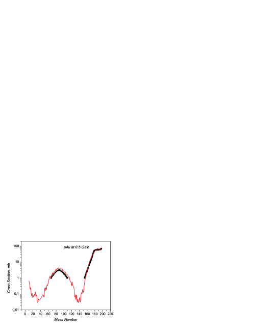
Figure 1: Mass distribution of residues produced in 0.5 GeV proton induced reaction on ¹⁹⁷Au; $p_{bond}=0.5$. Data are from paper[13].

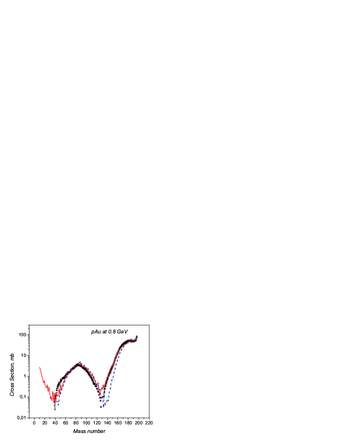
Figure 2: Mass distribution of residues in the reaction ¹⁹⁷Au + p at 800 A MeV; $p_{bond}=0.57$. Dashed curve is outcome of calculations without the contribution of multifragmentation channels . Data are taken from paper[14].

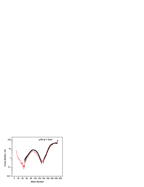
Figure 3: Mass distribution of residues in the reaction ²⁰⁸Pb + p at 1 A GeV; $p_{bond}=0.6$. Data are taken from paper[15].

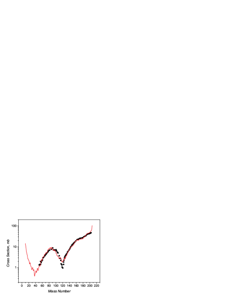
Figure 4: Mass distribution of residues in the reaction ²⁰⁸Pb + d at 1 A GeV; $p_{bond}=0.62$. Data are taken from paper[16].

Collisions of protons and light nuclei with heavy ions performed at GSI in inverse kinematics allows one to determine the production of residues prior to $\beta$ decay. This provides a good opportunity to compare the available data with theoretical models to achieve a better understanding of the mechanisms of reactions which is, today, far from satisfactory. Until now calculations have been performed by different versions of intranuclear cascade followed by the evaporation model.

Figure 5: Isotopic distribution of spallation residues in reaction ¹⁹⁷Au + p at 800 A MeV; $p_{bond}=0.57$. Data are taken from the paper[14].

Figure 6: Isotopic distribution of spallation residues in reaction ²⁰⁸Pb + p at 1 A GeV; $p_{bond}=0.6$. Data are from paper[15].

Figure 7: Isotopic distribution of spallation residues in reaction ²⁰⁸Pb + d at 1 A GeV; $p_{bond}=0.62$. Data are from the paper[16].

As seen from the previous section, our model also includes multifragmentation channels in the framework of the percolation approach. Here we define the values of the input parameters, which are the bond breaking probability, $p_{bond}(0)$, in Eq. (14) and the constant $c$ in Eq. (19). $p_{bond}(0)$ depends on the energy of the collision and the type of reaction. For a specific reaction, it is obvious that site and bond breaking probabilities are small at low energies and start growing with increasing energy, reaching constant values at the regime called ”limiting fragmentation”. Limiting fragmentation is reached at different energies for different reactions. Therefore, at low energies the dominating mechanisms of disintegration of excited remnants are evaporation and fission. As the energy of the collision grows, the contribution of multifragmentation processes increases, depending on the site and bond breaking probabilities. Since the number of broken sites is defined automatically during the development of the intranuclear cascade, only the bond breaking probability remains to be input as a parameter. For proton induced reactions, $p_{bond}(0)$ changes from 0, at an incident proton energy of a few tens of MeV, to 0.77 at the limiting fragmentation energy (3 – 4 GeV). With regard to the parameter $c$ in Eq. (19), its value is chosen to be 0.7, energy independent, for all types of reactions. Comparison of the model calculations for mass distributions in spallation reactions pAu at 0.5 and 0.8 GeV, pPb at 1 GeV, and dPb at 2 GeV are shown in Figs. 1 – 4. As seen from the figures, at energies lower than those corresponding to the limiting fragmentation regime, mass yield distributions of residues in proton-induced reactions have well-pronounced bell-shaped curves in the central part, corresponding to the contribution of fission channels. Evaporation channels give a dominating contribution in the right peak of the distribution with a plateau at high mass residues. The values of the level density parameters for evaporation and fission are taken to be 0.1A MeV^-1, the same for both and independent of the type of reaction and collision energy. Figures 5–7 show the isotopic distributions of residues produced in the following reactions: pAu at 0.8 GeV, pPb at 1 GeV and deuteron – Pb at 2 GeV. Calculated distributions are shifted toward neutron-rich isotopes for lighter residues. We think that underestimation of the proton–rich isotopes and overestimation of the neutron–rich isotopes could be corrected by better description of proton–neutron competition in fission–evaporation channels.

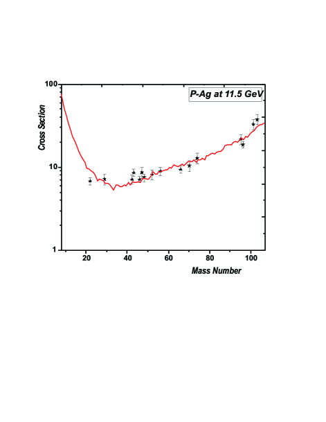
Figure 8: Mass distribution of fragments in the reaction p + ¹⁰⁸Ag at 11.5 GeV; $p_{bond}=0.77$. Data are taken from paper [17].

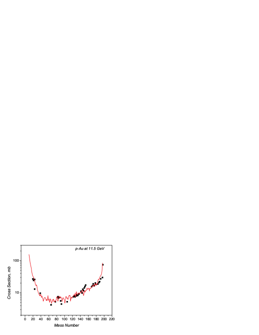
Figure 9: Mass distribution of fragments in the reaction p + ¹⁹⁷Au at 11.5 GeV; $p_{bond}=0.77$. Data are taken from paper [18].

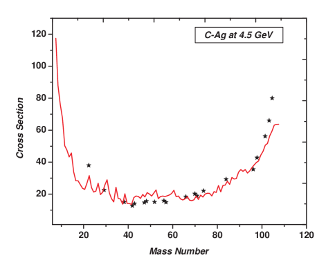
Figure 10: Mass distribution of fragments in the reaction ¹²C + ¹⁰⁸Ag at 4.5 A GeV; $p_{bond}=0.72$. Data are taken from paper [19].

As the bombarding energy increases, so does the contribution of multifragmentation channels and, correspondingly, the contribution of evaporation and fission channels decreases. This leads to filling of the dips at both sides of central bell-shaped curve and a decrease in the height of the right peak. As mentioned above, rising collision energy leads to an increasing number of broken sites and bonds in the nuclear lattices. This, in turn, results in increasing yield in multifragmentation channels. This tendency is already evident in reaction Au + p at 0.8 A GeV (Fig. 2). The mass distributions of fragments in proton- and carbon-induced reactions on Ag and Au at energies corresponding to the limiting fragmentation regime are shown in Figures 8 – 10.

6 Conclusions

A new version of the Modified Cascade Model for intermediate and high energy nucleus-nucleus collisions including multifragmentation channels has been developed. Colliding nuclei are represented as face–centered– cubic lattices. Multifragmentation is calculated in the framework of percolation theory with usage of a site–bond percolation model. This version is able to reproduce reasonably well both spallation and multifragmentation processes.

7 Appendix: Hadronic Event Generator

Monte Carlo simulation of inelastic events is performed in several steps. The first step in the generation of an exclusive event is the evaluation of the initial c.m. energy portion available for production of secondaries

$$W=\sum E_{i}=k\sqrt{s}$$ (20)

where $E_{i}$ is the energy of the i–th particle (excluding leading particles), $k$ is inelasticity. Fluctuation of the inelasticity from event to event leads to the distribution $P(k)$. There are no comparable theoretical methods for calculation of $P(k)$. It has been shown in Ref. [20] that one may fit the inelasticity distribution with a beta distribution

$$P(k,s)=k^{a-1}(1-k)^{b-1}/B(a,b)$$ (21)

$$B(a,b)=\Gamma(a)\Gamma(b)/\Gamma(a,b)$$ (22)

$$<k(s)>=a/(a+b)$$ (23)

where $\Gamma(a)$, $\Gamma(b)$ and $\Gamma(a,b)$ are gamma functions; $s$ is the dependence of $P(k,s)$ and $<k(s)>$ is enclosed in parameters $a$ and $b$. Up to the ISR energies one can neglect this $s$–dependence. In the second step the energy $W$ is distributed between secondary particles whose kinematical characteristics are generated in correspondence to a cylindrical phase space model. Parameters of the cylindrical phase space model are adjusted by comparing the results of simulation of pion–nucleon and nucleon–nucleon interactions with experimental data. The remaining part of c.m. energy $(1-k)\sqrt{s}$ is distributed between remnants of the interacting particles (so–called leading particles) according to the conservation of energy and momentum.

$$\overline{P}_{I}+\overline{P}_{II}=\sum\overline{P}_{i}$$ (24)

$$E_{I}+E_{II}=(1-k)\sqrt{s}$$ (25)

where $\overline{P}_{i}$ is the momentum of the $i$-th produced particle, and $\overline{P}_{I}$, $\overline{P}_{II}$ and $E_{I},E_{II}$, are momenta and energies of leading particles. Interacting nucleons (mesons) can transform into nucleons (mesons) and s – wave resonances ($\Delta$ – isobars and $\rho$, $\omega$ – mesons). Transition probabilities are calculated with the use of a one–pion-exchange (OPE) model.

References

- [1] W. Bauer et al., Nucl. Phys. A452 (1986) 699.
- [2] N.C. Chao and K. C. Chung, J.Phys. G: Nucl. Part. Phys. 17 (1991) 1851.
- [3] A.J. Santiago and K.C. Chung, J. Phys. G: Nucl. Part. Phys. 19 (1993) 349.
- [4] L. Pauling, Science 150 (1965) 297.
- [5] G. Anagnostatos, Can. J. Phys. 51 (1973) 998.
- [6] N.D. Cook, Atomkernenergie 28 (1976) 195; V. Dallacasa, Atomkernenergie 37 (1981) 143; V. Dallacasa and N.D. Cook, Nuovo Cim. A97 (1987) 157; ibid A97 (1987) 184; N.D. Cook and V. Dallacasa, Phys. Rev. C35 (1987) 1883.
- [7] G. Musulmanbekov, Proc.11th EMU01 Coll. Meeting, Dubna, May 11–13, 1992 (Ed. V. Bradnova), JINR, Dubna, 1992, p.288.
- [8] S.A. Krasnov et al., Czech. Jour. Phys., 46 (1996) 531.
- [9] N.D. Cook, Comp. in Phys. Mar/Apr, 1989, p.73.
- [10] N.D. Cook, J. Phys. G: Nucl. Part. Phys. 23 (1997) 1109.
- [11] V.S. Barashenkov and V.D. Toneev, Interactions of high energy particles and nulcei with atomic nuclei, Moscow, Atomizdat, 1972 (in russian).
- [12] X. Campi and J. Desbois, Proc. 23th Int. winter Meeting on Nucl. Phys., Bormio, 1985, p.707.
- [13] S. B. Kaufman et al., Phys. Rev., C22 (1980) 1897.
- [14] F. Rejmund et al., Nucl. Phys. A683 (2001) 540; J. Benlliure et al., Nucl. Phys. A683 (2001) 513.
- [15] W. Wlazlo et al., Phys. Rev. Lett. 84 (2000) 5736; T. Enqvist et al., Nucl. Phys., A686 (2001) 481.
- [16] J. Taïeb, PhD thesis, IPN Orsay, France, 2000.
- [17] G. English, N.T. Porile and E.P. Steinberg , Phys. Rev. C10 (1974) 2268.
- [18] S.B. Kaufman et al., Phys. Rev. C14 (1976) 1121.
- [19] P. Kozma et al., JINR–E2–94–380.
- [20] G.N. Fowler, R.M. Weiner and G. Wilk, Phys. Rev. Lett. 55 (1985) 173.