Local scale transformations and extended matter distributions in nuclei

Abstract

Local scale transformations are made to vary the long range properties of harmonic oscillator orbitals conventionally used in model structure calculations of nuclear systems. The transformations ensure that those oscillator states asymptotically have exponentially decaying forms consistent with chosen single nucleon binding energies, leaving the structure essentially unchanged within the body of the nucleus. Application has been made to the radioactive nuclei ^6,8He and ¹¹Li and the resulting wave functions are used to generate $g$-folding optical potentials for elastic scattering of those ions from hydrogen. As a consistency test, application has been made to form wave functions for ⁴⁰Ca and they have been used also to specify relevant proton-⁴⁰Ca optical potentials with which elastic scattering has been predicted. The need for appropriate specifications of single particle binding energies in exotic nuclei is discussed.

I Introduction

A topic of current interest is the description of the structures of exotic nuclei, especially as one approaches the drip lines. The light mass neutron/proton rich nuclei are particularly suited for study as a number of these nuclei can be formed as radioactive beams with which experiments to determine their scattering cross sections can be made. Their scattering from Hydrogen targets is of special interest as this is currently one of the best means by which the densities of such nuclei may be studied microscopically. That is achievable as predictions can be made of nucleon-nucleus ($NA$) scattering (elastic and low excitation inelastic) with a folding model scheme Amos et al. (2000); Karataglidis et al. (2002), in a manner consistent with that employed for electron scattering. Such allows for a sensitive assessment of the matter densities of nuclei, as was demonstrated in the case of ²⁰⁸Pb Karataglidis et al. (2002). That is the case also for the scattering of radioactive ions from Hydrogen, as inverse kinematics equates the process to the scattering of energetic protons from the ions as targets. However, to make such predictions Amos et al. (2000), three basic aspects of the system under investigation are required. Where possible, these properties must be determined independently of the proton-nucleus ($pA$) scattering system being studied.

One must start with a credible effective (in-medium) two-nucleon ($NN$) interaction. Numerous analyses (to 300 MeV) now suggest that such can be deduced from $NN$ $g$ matrices; solutions of Bruckner-Bethe-Goldstone (BBG) equations based upon any realistic (free) $NN$ potential. With such effective interactions, analyses of $NA$ scattering data become tests of the description of the target nucleus, namely of its proton and neutron densities.

The second ingredient is the set of those densities. In the procedure we adopt, they are determined from the folding of one-body density matrix elements (OBDME) and single particle (SP) wave functions, both of which should be obtained from credible models of structure. Such are normally large scale structure models which describe well the ground state properties (and low-lying excitation spectra if pertinent) of the nucleus in question.

The third ingredient is the specification of the SP wave functions and it is that with which this paper is concerned. For the moment let us presume that SP wave functions can be specified appropriately so that in making a $g$-folding optical potential Amos et al. (2000) there is nothing left to be parameterized as such. When all elements have been chosen with care, namely when appropriate modifications to the (free space) interactions between the projectile nucleon and each and every target nucleon caused by the nuclear medium are made, and when OBDME and SP wave functions which well describe the target are used (for stable nuclei that means spectra, electromagnetic moments and transition rates, and electron scattering form factors), then predictions of the scattering of nucleons from such nuclear targets can be, and have been, made of angular and integral observables Amos et al. (2000). That includes spin-dependent angular observables. Furthermore, analyses of data from the scattering of protons from ²⁰⁸Pb Karataglidis et al. (2002) clearly indicated a preferential model of the structure of that nucleus so that ²⁰⁸Pb should have a neutron skin thickness of 0.17 fm.

With radioactive nuclei, however, there are far less known static properties and no electron scattering data to complement, and to constrain analyses of, the existent limited hadron scattering data. Of course structure models for those nuclei are a major field of study currently and, of note for the studies we report, several groups have made shell model calculations of the light mass radioactive nuclei, ^6,8He and ¹¹Li. Of those, Navrátil and Barrett Navratil and Barrett (1996, 1998) have made large-space calculations (up to $6\hbar\omega$ in the model space) using interactions obtained directly from the $NN$ $G$ matrices which have the Reid93 $NN$ interaction as their base. Also Karataglidis et al. Karataglidis et al. (2000) calculated wave functions for ^6,8He within a complete $(0+2+4)\hbar\omega$ model space using the $G$ matrix interaction of Zheng et al. Zheng et al. (1995) based on the Nijmegen III $NN$ interaction. They Karataglidis et al. (1997a) also defined wave functions for ¹¹Li using a complete $(0+2)\hbar\omega$ model space and fitted potentials. From those wave functions the OBDME to use in the descriptions of both proton elastic scattering and of the ($\gamma,\pi^{+}$) reaction (in the case of ⁶He only Karataglidis et al. (2000)) were determined. Both elastic proton scattering and charged pion photoproduction reactions probe the microscopic structure of the nucleus in a way that initial states are preserved in the reaction so that the analyses of scattering or reaction data should not be complicated by the need to describe details of reaction products. With that assumption, the analyses Karataglidis et al. (2000) confirmed ¹¹Li to be a halo nucleus while both ⁸He and ⁹Li are not. The analysis of the (then) available data on ⁶He did not allow a conclusion on the halo structure in ⁶He to be made. But the subsequent measurement and analysis of $p$-⁶He scattering by Lagoyannis et al. Lagoyannis et al. (2001), and later by Stepantsov et al. Stepantsov et al. (2002), have confirmed that ⁶He has an extended neutron distribution consistent with a halo.

Frequently, in analyses of scattering data, harmonic oscillator (HO) wave functions have been chosen to describe single nucleon bound states in nuclei. A more realistic representation may be Woods-Saxon (WS) functions, as found for ¹²C Karataglidis et al. (1995) for example. With the OBDME determined from $(0+2)\hbar\omega$ shell model wave functions and the single nucleon bound states appropriately specified, electron scattering form factors from both the elastic and inelastic scattering of electrons from ¹²C then were well fit Karataglidis et al. (1995). To estimate effects of any halo attribute in the nucleus also requires variation of the SP wave functions from the HO set defined by (large-space) shell model calculations. Such has been attempted also using WS wave functions, as originally used in the analysis of the strong $E1$ transition in ¹¹Be by Millener et al. Millener et al. (1983). In such cases no constraining electron scattering data exist. Even if there were, electron scattering data primarily are a measure of the proton distribution of the nucleus. Little information is obtained directly about the neutron densities from such data.

In the case of a neutron halo, a specification of the optical potential requires the use of wave functions with the appropriate long range behavior. Normally, this is done with the use of WS functions, somewhat artificially. Indeed to force a halo structure on nuclei within the traditional (bound state) shell model, with no coupling to the continuum, requires bound state WS potentials to be adjusted so that certain shell model states are weakly bound. A halo structure was given to ⁶He Karataglidis et al. (2000), for example, by setting the neutron $0p$ shell binding at 2 MeV (near the single neutron separation energy of 1.8 MeV Tilley et al. (2000)) and the $sd$ shell and higher states at 0.5 MeV (as dictated within the spirit of the shell model single particle spectrum). No single WS potential parametrization can give all of those bound states having the relevant binding energies.

However, a procedure exists that ensures bound state wave functions will have asymptotically an appropriate exponential behavior Petkov and Stoitsov (1983); Stoitsov et al. (1998); Pittel and Stoitsov (2001) whatever its originating form and without sacrificing, too severely, bulk internal character of shell model structure. That involves making a local scale transformation (LST) of the coordinate variable of the bound state wave functions used in structure calculations (even if they have been so used only implicitly). Namely, given wave functions which adequately describe bulk properties, we modify the tails of HO SP wave functions, as specified by the requisite shell model, for example, in the least artificial way to ensure compatibility with whatever choice is made for single nucleon binding energies. This is of special interest for “halo” nuclei, or candidates as such.

Herein, Section II briefly recalls the properties of some such special nuclei. Then in Sections III and IV we explain the formalism of the scale transform and give its justification. The results of application of the LST wave functions to an analysis of proton-nucleus (nucleus-Hydrogen) scattering are presented in Section V. Concluding remarks follow thereafter.

II Some aspects of the nuclei ${}^{6,8}\text{He}$ and ${}^{11}\text{Li}$

Shell model calculations of ^6,8He and ¹¹Li have been made to determine the nucleon shell occupancies $n_{i}$ to be used in calculations of the optical potentials for the elastic scattering of beams of those ions from Hydrogen targets. By inverse kinematics that equates to proton scattering from the ions themselves. We have used the information from shell model calculations made for earlier studies Karataglidis et al. (1997a); Karataglidis et al. (2000); Amos et al. (2000); calculations in which all the nucleons of ^6,8He and ¹¹Li were taken as active (the so-called “no core” shell model). Specifically we use the structure information given from those calculations of ^6,8He made in a complete $(0+2+4)\hbar\omega$ model space, and for ¹¹Li made in the smaller $(0+2)\hbar\omega$ model space. The latter space limitation arose from the dimensionality increasing with mass for a given space. While the ^6,8He information came from calculations made using the $G$ matrix interaction of Zheng et al. Zheng et al. (1995), the WBP interaction Warburton and Brown (1992) was used for ¹¹Li.

To utilize the LST, we list, in Table 1, a set of estimated

Table 1: Estimated binding energies (in MeV) for single nucleon orbits in ^6,8He and ¹¹Li.

Orbit	6He		8He		11Li
	proton	neutron	proton	neutron	proton	neutron
$0s_{\frac{1}{2}}$	24	24	24	24	33	33
$0p_{\frac{3}{2}}$	16.5	4.0	16.5	14.5	15.7	7.7
$0p_{\frac{1}{2}}$	15.5	2.0	15.5	13.5	13.8	5.0
$0d_{\frac{5}{2}}$	7.0	2.0	7.0	5.0	2.0	0.8
$0d_{\frac{3}{2}}$	5.0	2.0	5.0	4.0	1.5	0.8
$1s_{\frac{1}{2}}$	7.0	2.0	7.0	5.0	2.8	0.8
$0f-1p$	2.0	2.0	2.0	2.0	0.8	0.8

binding energies for nucleons in the $0s$ to $0f$–$1p$ orbits of the exotic nuclei of interest. We stress that this set is used for illustration; it should not be taken as definitive. In defining this set we have been guided by the systematics of single particle energies Hodgson (1994), on what WS functions were needed to match form factors from electron scattering from ^6,7Li Karataglidis et al. (1997b), and from seeking rms values assessed from other data analyses. We were also guided by our previous work involving using WS functions in the descriptions of exotic nuclei Karataglidis et al. (1997a); Karataglidis et al. (2000). Note also that the choice is dictated by the ordering of the single particle states in the underlying shell model; this approach differs from that taken by Millener et al. Millener et al. (1983), where the factorization of the OBDME in terms of spectroscopic factors connecting to the spectrum of the $(A-1)$ nucleus make the binding energies change with the relevant component configurations of the wave function.

In Table 2 the orbit occupancies determined from our chosen shell model calculations, and up to the $sd$ shell, are listed. With those occupancies and with a set of SP (proton or neutron) radial wave functions $\varphi_{i}(r)$, we define a (proton or neutron) density profile by

$$\rho_{p/n}(r)=\sum_{i}n_{i}\int d\Omega\;\varphi_{i}^{\ast}(\bm{r})\varphi_{i}(\bm{r})$$ (1)

where these densities are normalized according to

$$\int_{0}^{\infty}\rho_{p}(r)r^{2}dr=Z\text{\ \ and\ \ }\int_{0}^{\infty}\rho_{n}(r)r^{2}dr=N\;.$$ (2)

Table 2: Shell occupancies and rms radii from shell model calculations.

Orbit	6He		8He		11Li
	proton	neutron	proton	neutron	proton	neutron
$0s_{\frac{1}{2}}$	1.821	1.886	1.836	1.915	1.994	1.998
$0p_{\frac{3}{2}}$	0.036	1.718	0.035	3.575	0.929	3.699
$0p_{\frac{1}{2}}$	0.036	0.262	0.038	0.329	0.037	1.474
$0d_{\frac{5}{2}}$	0.023	0.017	0.016	0.028	0.014	0.383
$0d_{\frac{3}{2}}$	0.029	0.024	0.018	0.027	0.019	0.068
$1s_{\frac{1}{2}}$	0.031	0.034	0.035	0.036	0.006	0.373
higher	0.024	0.059	0.022	0.090	0.001	0.005
$b$ (fm)	1.6	1.6	1.6	1.6	1.6	1.6
$r_{\text{rms}}$ (fm)	2.11 (2.27)	2.59 (3.58)	2.09 (2.20)	2.69 (2.79)	2.16 (2.37)	2.46 (4.45)
Mass $r_{\text{rms}}$ (fm)	2.44 (3.21)		2.55 (2.66)		2.38 (3.99)

Listed also are the oscillator lengths used in those shell model calculations and they lead to the rms radii given in the second last line of the table. The numbers given in brackets are the rms values found using the LST functions, that we define (and discuss) later, using the binding energies in Table 1. In the bottom line we list the rms radii for the entire nuclear mass, again with the values resulting from using the LST wave functions shown in the brackets. We consider first the shell model results here noting that the proton and neutron rms radii differ for each nuclei thereby naturally identifying a neutron skin for each. However the rms radii obtained for ⁶He and ¹¹Li do not define the neutron halo character that both are expected to have. (That will always be the case when HO functions are used.) The proton rms radius obtained from the LST calculation is consistent with the oscillator result in each case. The neutron rms radii for ⁶He and ¹¹Li as obtained from the LST model are higher than the oscillator result but are commensurate with those obtained from the WS and Glauber models Amos et al. (2000). There is agreement in the neutron radii obtained for ⁸He from both the oscillator and LST as consistent with this nucleus being a neutron skin Karataglidis et al. (2000). The reaction cross sections for each nucleus are listed in Table 3,

Table 3: Reaction cross sections (in mb) at the list energy (MeV) as obtained from the HO and LST ($m=8$) model calculations.

Nucleus	Energy	HO	LST
6He	40	321	441
8He	71	280	293
11Li	62	343	447

with the energies listed reflecting the results for the differential cross sections discussed later. In the case of ⁶He, there is an experimental value de Vismes et al. (2002) of $410\pm 21$ mb at 36.2 MeV. The (concocted halo) WS result at 40 MeV is 406 mb Lagoyannis et al. (2001). The LST result of 441 mb remains in better agreement with these values than the HO result (353 mb Lagoyannis et al. (2001)); the slight discrepancy is due to the larger rms radius compared to that found from a Glauber model analysis of the interaction cross section [$2.71\pm 0.04$ fm Al-Khalili et al. (1996)]. A similarly small overestimation in the rms radius is observed for ¹¹Li, for which the radius estimated from the interaction cross section is $3.53\pm 0.10$ fm Al-Khalili et al. (1996), and we expect that a measurement of that reaction cross section would fall below our prediction. Nevertheless, we are encouraged by the result for ⁸He where the reaction cross section from the LST model is similar to the HO result as consistent with ⁸He being a skin nucleus.

Thus it is clear that the choice of SP wave functions is crucial to explain observed scattering data and it seems that an important factor with that choice is the binding energy for each and every bound nucleon. For the halo orbits, that binding will be weak and the contributions from those orbits will be small, commensurate with the (usually) small occupation numbers associated with them. Some control is available by requiring that the rms radii be well predicted. Only with the ¹¹Li case is the $1s$ wave function of some importance but it is more significant to have a form for this that is extended noticeably from the Gaussian function than it is to have a precise binding energy — at least within the context of the present paper. As has been noted Amos et al. (2000); Lagoyannis et al. (2001); Stepantsov et al. (2002), it is the reduction of the neutron density within the core of the neutron halo nuclei that is significant in the analyses of proton scattering. Heavy ion scattering reflect longer range properties and so we look forward to use of the LST scheme to define density profiles, etc., that can be used in such (heavy ion) reaction studies. The tabulated values thus are a base input in a study of LSTs to see if the HO functions, used in the shell model calculations to give the OBDME, may be adapted to better describe the matter profiles and properties of these nuclei. The present study of the LST is exploratory and the calculated matter densities within this model are not given as “final” determinations.

III The local scale transformation

As given previously Stoitsov et al. (1998); Pittel and Stoitsov (2001), an LST Petkov and Stoitsov (1983) of the form, $r=f(s)$, replaces an original wave function $u(r)$ by a new one $v(r)$ defined by the isometric transform,

$$v(r)=\sqrt{\frac{df}{dr}}\,u\left[f(r)\right],$$ (3)

where $f(r)$ must be real and monotonically increasing when $r$ runs from 0 to $\infty$. Also, two boundary conditions are in order, namely $f(0)=0$ and $f(r)\rightarrow\infty$ as $r\rightarrow\infty$. The isometry of this mapping of wave functions $u$ into wave functions $v$ is obvious since scalar products are conserved. Indeed, let $u$ and $u^{\prime}$ be two initial wave functions and consider their respective images $v$ and $v^{\prime}$ under the transform. Then, trivially,

$$\int_{0}^{\infty}ds\,v(s)v^{\prime}(s)=\int_{0}^{\infty}ds\,\frac{df}{ds}u\left[f(s)\right]u^{\prime}\left[f(s)\right]=\int_{0}^{\infty}dr\,u(r)u^{\prime}(r),$$ (4)

under the obvious change of integration variable $r=f(s)$. With metrics for radial wave functions where one uses an integral $\int_{0}^{\infty}r^{2}dr$, the transform, Eq. (3), must be slightly modified to,

$$v(r)=\frac{f(r)}{r}\sqrt{\frac{df}{dr}}u\left[f(r)\right]=s(r)u\left[f(r)\right]\;,$$ (5)

where $s(r)$ is the wave function scale.

We are interested specifically in converting the usual shell model (HO) orbitals into ones that have a physical, exponential decrease. Let $b$ and $\mu$ denote the HO length and the (bare) nucleon mass respectively, and consider an orbital that is bound by an energy $\varepsilon$; the binding being counted as a positive number. If we neglect sub-dominant modulations brought by the polynomials present in the HO functions and, possibly, by the derivative $df/dr$, the choice of $f$ must induce the change in structure

$$\exp{\left(-\frac{r^{2}}{2b^{2}}\right)}\Rightarrow\exp{\left(-r\sqrt{\frac{2\mu\varepsilon}{\hbar^{2}}}\right)}\;.$$ (6)

Hence, when $r\rightarrow\infty,$ we must constrain $f$ by

$$f(r)\rightarrow\gamma\sqrt{r},\text{ with }\gamma=b\left[\frac{8\mu\varepsilon}{\hbar^{2}}\right]^{\frac{1}{4}}.$$ (7)

Simultaneously, it seems best to set $f(r)\rightarrow r$ when $r\rightarrow 0$. This choice leaves the interior of the orbitals essentially unchanged. Accordingly, the transition between the “inner, intact” regime, $f(r)=r$, and the “outer, tail compatibility” regime, $f(r)=\gamma\sqrt{r}$, must occur about the point $r=r_{t}=\gamma^{2}$, which we define as the transition radius. But a choice will need to be made between two solution conditions, namely

(i)

extension of the linear regime to respect the initial wave function as much as possible, and

(ii)

fix the transition according to the SP separation energies, as soon as $r$ is of the order $\gamma^{2}$ for each individual orbital.

Geometrically, condition (i) consists in keeping a straight line for $f(r)$, overshooting the $\gamma\sqrt{r}$ parabola, then bending the formerly straight line slowly to reach the parabola from upper values. The second choice consists of an unbiased interpolation between straight line and parabola, thus deviating earlier from the straight line. In that case $f(r)$ will always lie below both the line and the parabola limits and its derivative will remain positive definite and monotonically decreasing. Thus under under condition (ii) the normalization in Eq. (5) is always real and the transform gives a new function that gains the larger orbit probability amplitude at long range (exponential rather than Gaussian) at the expense primarily of the surface region Gaussian amplitudes. We believe that the condition (ii) features are sensible ones to have with the transform, especially as a negative gradient (and thereby indeterminate normalization) is not prevented with condition (i).

IV The harmonic mean form

Solution condition (ii) is met if we use a harmonic mean form for the LST, namely

$$f(r)=\left[\frac{1}{\left(\frac{1}{r}\right)^{m}+\left(\frac{1}{\gamma\sqrt{r}}\right)^{m}}\right]^{\frac{1}{m}}\ .$$ (8)

This form has the added attractive character in that it depends primarily upon the chosen SP binding energies. The order $m$ controls how sharply the transform alters the coordinate between the limits. We present, empirically, the results for $f(r)$, its derivative $\frac{df(r)}{dr}$ and of the wave function scale $s(r)$ for harmonic mean forms with $m=4$ and 8 in the next two figures. These test calculations were made using $b=1.6$ fm and a mass of 1. In both figures, the results shown by the solid and dashed curves respectively are for binding energies of 1 and 20 MeV. In the top segment of these figures, the dot-dash curves display the parabolas $f=\gamma\sqrt{r}$ for each orbital while the dotted line is the central limit of $f=r$. In the middle segment of each figure, the derivatives of the transformations are displayed. In the bottom panel the scaling function with which the transformed wave function $u\left[f(r)\right]$ is multiplied in Eq. (5) is shown.

For both the $m=4$ and $m=8$ harmonic mean cases, portrayed in Figs. 1 and 2 respectively, a weaker

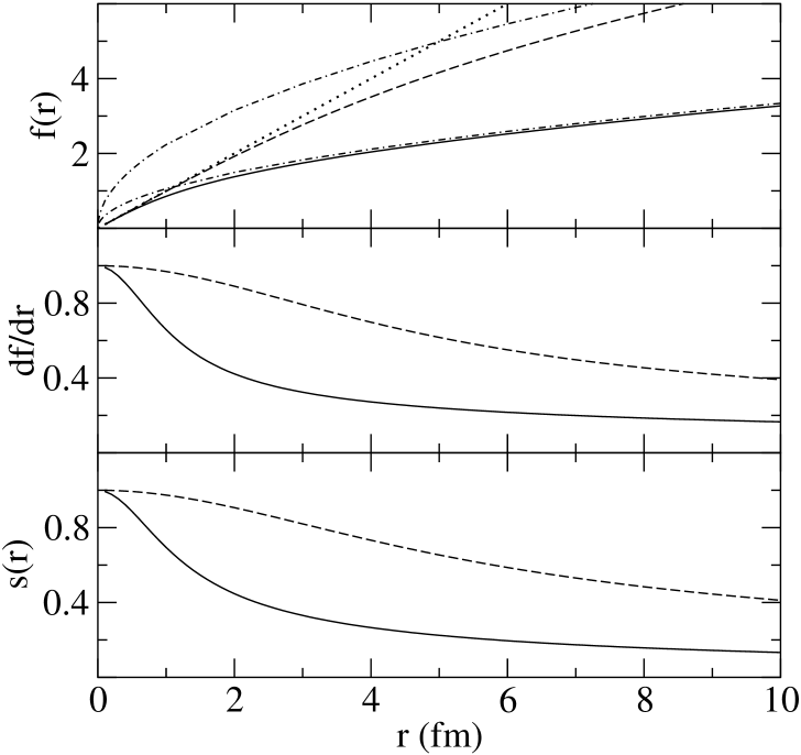
Figure 1: The $m=4$ harmonic mean transform results for binding energies of 1 MeV (solid curves) compared with those for a binding energy of 20 MeV (dashed curves). The limit transform functions also are shown in the top panel by the dotted curve [$f(r)=r$] and by the two dot-dashed curves [$f(r)=\gamma\sqrt{r}$].

Figure 2: The transform functions as given in Fig. 1, but now for $m=8$.

binding induces an earlier transition from the linear to the parabolic regime. The derivatives also vary monotonically to give scaling functions that do so as well. (For the sake of completeness, we investigated several values of $m$, of which $m=4$ and $m=8$ only were chosen for the figures.) Therein it is readily seen that with larger $m$ the interpolating curve follows initially the straight line limit from the origin before smoothly, but more quickly, varying as the parabola. Actually, if $m\rightarrow\infty$, then $f(r)$ becomes strictly linear until the intersection point between the two regimes and then strictly parabolic beyond. At this limit however, the continuity in the derivative of $f$ is lost. That loss would make our transformed wave function have a discontinuity as well, and was a reason for our choice of moderate values of $m$ for calculations of the nuclear wave functions to be used later.

The key role played by the binding energy in modulating the wave functions is apparent from these diagrams as well. Besides the transform effect of changing Gaussian radial distributions to exponentials with the appropriately defined exponents, the scaling functions depicted in the bottom segments show that, with deeper binding, the interior character of a shell model wave function would be retained more than those for weaker binding. Also the increase of power (from $m=4$ to 8) causes the variation to be more surface oriented. That is a consequence of the transform remaining closer to the linear limit until the break point, which increases in radius with binding energy (larger $\gamma$). It is important to note that the normalising scale function, $s(r)$, tends slowly to zero as $r$ increases which has a consequence for the densities obtained.

We show now the cases for three exotic nuclei, ^6,8He and ¹¹Li. The last, ¹¹Li, is a special case as we need to address with it a question of non-orthogonality. It, of the three exotic light mass nuclei considered, has a sizable $1s_{\frac{1}{2}}$ neutron shell occupancy, as consistent with its $s$-wave halo.

IV.1 The case of ⁶He

In Figs. 3, 4,

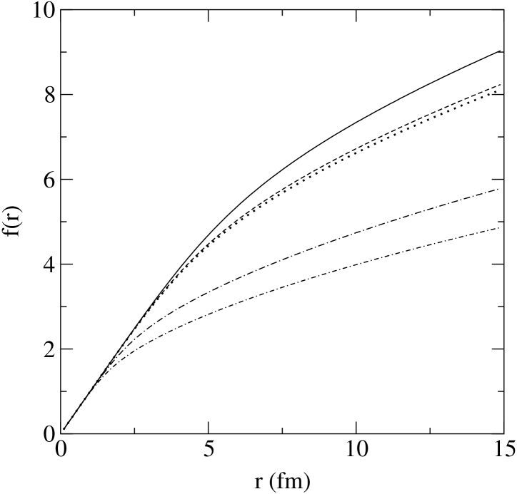
Figure 3: The $m=8$ harmonic mean coordinate transform functions for the orbits of ⁶He found using the binding energies listed in Table 1. The transforms for the $0s_{\frac{1}{2}}$, $0p_{\frac{3}{2}}$, and $0p_{\frac{1}{2}}$ protons are shown from the top by the solid, dashed, and dotted curves, while those of $0p$-shell neutrons bound by 4 and 2 MeV are depicted by the dot-dashed and double-dot-dashed lines respectively.

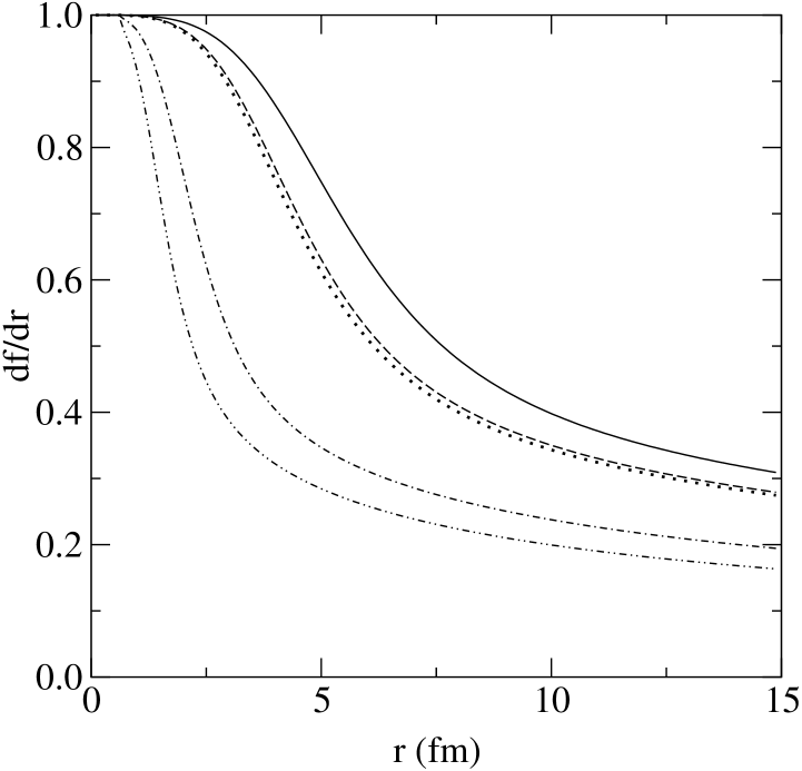
Figure 4: As for Fig. 3 but for the derivatives, $\frac{df(r)}{dr}$.

5, and 6, we show the

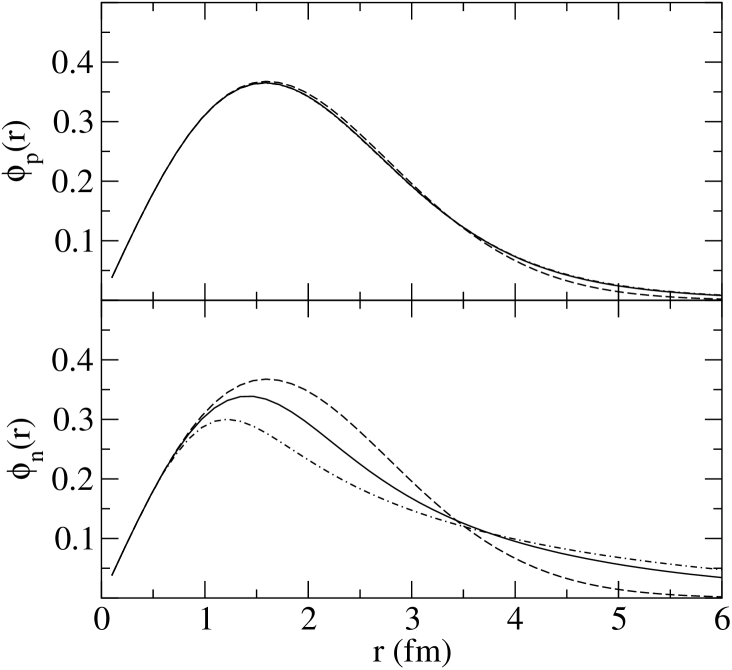
Figure 5: The $p$-wave orbit functions for ⁶He. The LST results are shown by the solid ($0p_{\frac{3}{2}}$) and dot-dashed ($0p_{\frac{1}{2}}$) curves for various binding energy values as stated in the text while the HO wave functions are shown by the dashed curves.

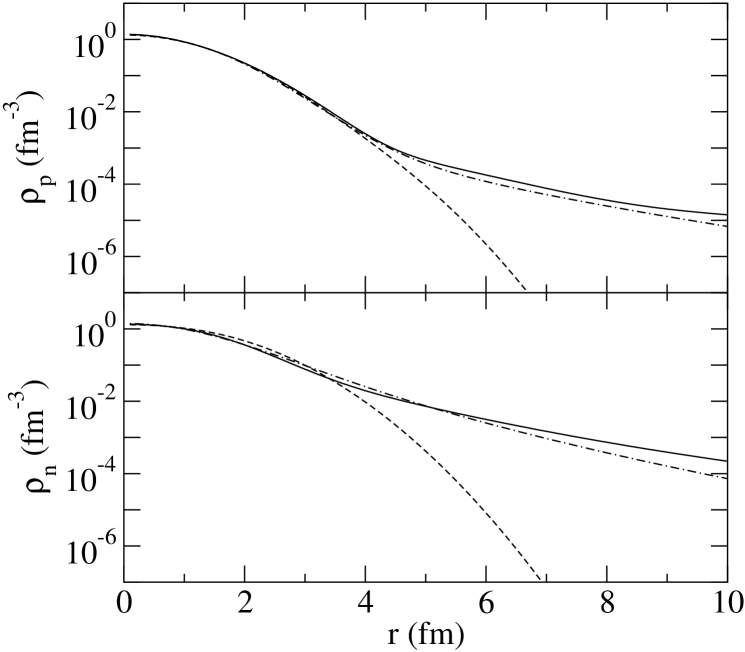
Figure 6: The proton (top) and neutron (bottom) densities for ⁶He. The HO, LST, and WS results are portrayed by the dashed, solid and dot-dashed curves, respectively.

harmonic mean ($m=8$) results for the transformation functions and their derivatives, the individual wave functions, and the densities for ⁶He. In Figs. 3 and 4, the coordinate transform functions $f(r)$ and their derivatives $\frac{df(r)}{dr}$ for the $0s_{\frac{1}{2}}$ through $0p_{\frac{1}{2}}$ wave functions for ⁶He with the binding energies listed in Table 1, are shown. The identification of the different orbit results is given in the figure caption. Since the scale factor is quite similar to the derivative functions for most radii of interest they are not shown. However, from the shapes of the derivatives, the $0s$ orbit will remain essentially unchanged inside the nuclear volume, such as it is for ⁶He, while the $0p$ orbits will be influenced more, especially the neutron orbits. The degree to which this is the case is shown in Fig. 5. The top panel gives two $0p$ wave functions generated from that oscillator function using the $m=8$ harmonic mean LSTs with binding energies of of Table 1. Note that for the protons (top panel) there is only a very slight change to effect the exponential forms with a reduction of the amplitudes for radii in the range 1 to 3 fm. The weaker bound (neutron) orbits in contrast are much varied from the starting HO form with a reduction through the nuclear interior to give the strong enhancement asymptotically. Thus an extended neutron (halo) distribution can be formed by summation over the orbit occupancies. The results are shown in Fig. 6 with proton and neutron matter densities in the top and bottom segments, respectively. The HO, WS, and LST results are portrayed by the dashed, dot-dashed and solid curves, respectively. The neutron halo is clearly established by both the WS and LST model results as compared to that from the HO model. Note that the asymptotic properties of the wave functions, and therefore densities, tend slowly towards an exponential form. From the LST, this is due to the behavior of the scaling function for each orbital, $s(r)$, tending to zero only as $r^{-3/4}$. The consequence of that extension in the neutron density is an extension also for the proton density, though not quite as strong. This stems from the addition of small contributions from the loose binding in the proton SP orbits folded with the small occupation numbers for the proton orbits above the $0p$ shell, all of which are of comparable size. That dilution of the proton density by an extensive neutron density, due to the effects of the $NN$ force, is expected in heavy, neutron-rich, nuclei. This is consistent with the slightly larger proton rms radius obtained from the LST model, as compared to the oscillator result.

IV.2 The case of ⁸He

We consider ⁸He a test case since it is reasonably well established that this nucleus does not have a neutron halo. Rather, the excess neutron number creates a skin, whose properties have been established in analyses of proton and heavy-ion scattering data (Karataglidis et al. (2000) and references cited therein). Starting with the shell model results (OBDME and SP wave functions) and an oscillator length of 1.6 fm, the density profiles for ⁸He given the binding energies listed in Table 1 are shown in Fig. 7. Proton (neutron) densities are shown in

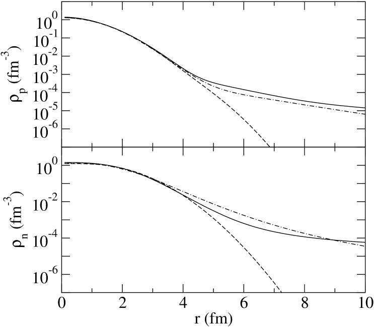
Figure 7: The proton (top) and neutron (bottom) densities for ⁸He. The HO, LST, and WS results are portrayed by the dashed, solid, and dot-dashed curves, respectively.

the top (bottom) segment with those found using the HO, WS, and LST functions displayed by the dashed, dot-dashed and solid lines respectively. As with the WS and LST densities in ⁶He, extensions of both the neutron and proton densities are observed, although the neutron densities are not as strong at 10 fm as with ⁶He. This is consistent with the understanding of ⁶He having a neutron halo and ⁸He having a neutron skin. Note also that the results for the rms radius and reaction cross section for ⁸He obtained from the LST model are also consistent with a neutron skin description of ⁸He.

IV.3 The case of ¹¹Li – a two $s$ orbit problem

For the case of ¹¹Li, the shell model calculations Karataglidis et al. (1995) give dominant occupancies for the orbitals as listed in Table 2 and the binding energies that were taken to calculate WS bound state functions with which a neutron halo was created Lagoyannis et al. (2001) are listed in Table 1. In this case there are two $s$ orbitals and the schemes used previously to define a “halo” did not retain orthogonality of those orbits, nor does the LST process set out above. But that can be rectified.

The case where there are several orbitals with the same $\{ljm\}$ quantum numbers can be handled as follows. Assume, for the sake of argument, that there are three $s_{1/2}$ orbitals, namely $0s_{1/2}$, $1s_{1/2}$, and $2s_{1/2}$, with respective (positive) binding energies $\varepsilon_{0}>\varepsilon_{1}>\varepsilon_{2}$, and corresponding parameters $\gamma_{0}>\gamma_{1}>\gamma_{2}$, according to Eq. (7). Then LSTs parameterized independently by $\gamma_{0}$, $\gamma_{1}$, and $\gamma_{2}$ convert the HO functions into orbitals $\left|0\right\rangle$, $\left|1\right\rangle$, and $\left|2\right\rangle$ which are normalized but are not orthogonal. It is a trivial matter to subtract from $\left|1\right\rangle$ that amount of $\left|0\right\rangle$ necessary to regain orthogonality, and to renormalize the resultant new orbit vector $\left|1^{\prime}\right\rangle$. Notice that this resultant state will have a long range aspect still driven by $\gamma_{1}$ since the subtraction of a component proportional to $\left|0\right\rangle$ contains a (much) shorter range tail driven by $\gamma_{0}.$ In turn, it is trivial to orthogonalize $\left|2\right\rangle$ to $\left|0\right\rangle$ and $\left|1^{\prime}\right\rangle$ and renormalize the result into an orbital $\left|2^{\prime}\right\rangle$; the tail of which is still governed by $\gamma_{2}$. This process is iterative.

The LST functions for the set of binding energies for ¹¹Li listed in Table 1, and for $m=8$, are shown in Fig. 8. For the $0s$ case the

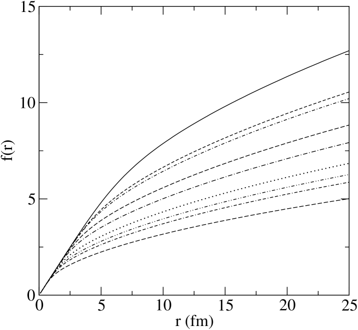
Figure 8: The LSTs for states in ¹¹Li obtained using the binding energies of Table 1. Curves are identified in the text.

proton and neutron transform function is identical and is the top (solid) curve in this figure. The transform functions for the $0p$-shell are different as indicated by the shallower binding for the neutrons. The functions for the $0p_{\frac{3}{2}}$ and $0p_{\frac{1}{2}}$ orbits are represented by the dashed and dot-dashed lines, respectively. The higher lying set are those for the protons. The remaining curves are the transforms for the proton: the $sd$ states as shown in descending sequence for the $1s_{\frac{1}{2}}$ (dotted), the $0d_{\frac{5}{2}}$ (double-dot-dashed), and the $0d_{\frac{3}{2}}$ (dot-double-dashed) proton states. The lowest (long-dashed) curve is the transform function for the three $1s-0d$ neutron states as each was chosen to have a binding energy of 0.8 MeV in these calculations.

The $s$-state wave functions that result after re-orthogonalization are shown in Fig. 9. Because the proton and

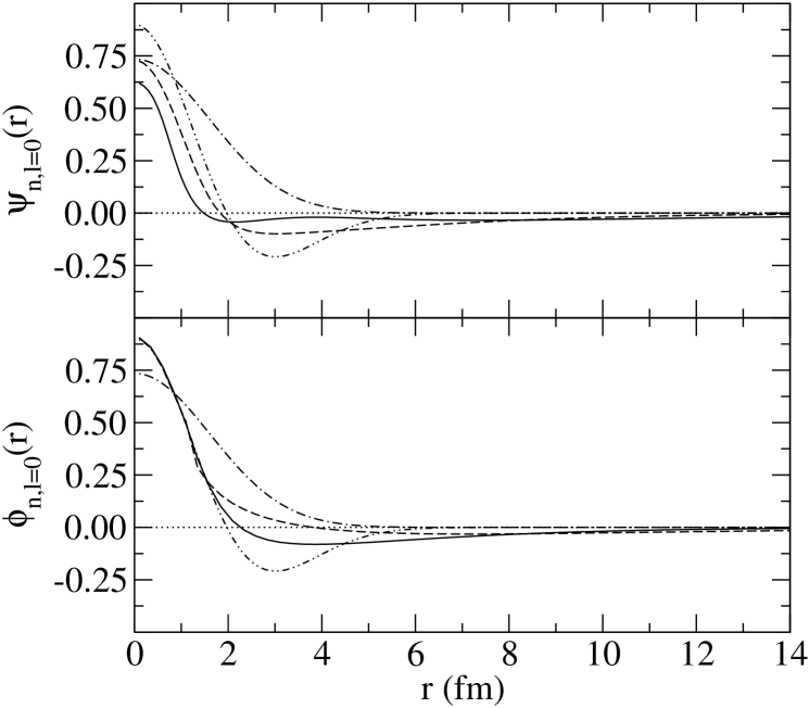
Figure 9: The $s$-wave functions for ¹¹Li. Harmonic oscillator functions are shown by the dot-dashed $(0s)$ and double-dot-dashed $(1s)$ curves in both segments. Proton and neutron LST-transformed $1s$ functions are given by the solid and dashed lines, respectively. The use of the LST alone gives the wave functions displayed in the bottom segment which, after orthogonalization, become those given in the upper segment.

neutron $0s$ orbits were both chosen to be bound by 33 MeV there is little change to their wave functions from that of the starting HO function. Of course the long range form differs: the transformed wave functions have an exponential character while the HO is Gaussian. But those differences cannot be discerned on the scales used in Fig 9. Those $0s$ HO wave functions are shown in both the upper and lower parts of this figure by the dot-dashed curve. The $1s$ states change markedly not only by virtue of the LST but also with re-orthogonalization. Due to the LST alone, wave functions shown in the bottom panel of Fig. 9 result. After orthogonalization, the wave functions displayed in the top panel result. In both panels the transformed $1s$ wave functions determined with a binding energy of 2.8 MeV (proton) and by 0.8 MeV (neutron) binding energy are shown by the solid and dashed curves respectively. Not only are the spatial variations of the transformed wave functions quite different from that of the initial $1s$ oscillator (bottom panel) as the transform varies the HO to get the relatively weak binding form of the exponentials, but also those changes are altered with the central radial values of the LST functions markedly reduced under the constraint that the $0s$ and $1s$ results be orthonormal. Indeed both the proton and neutron $1s$ orbit functions are extended, though by virtue of its weaker binding the neutron one is the more so. Then with the rather large occupancy of neutrons in the $1s$ orbit the neutron matter profile has the character of a neutron halo.

Diverse neutron matter densities are shown in Fig. 10.

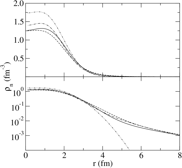
Figure 10: The neutron matter densities in ¹¹Li given by the HO (double-dot-dashed), the $m=8$ harmonic mean transformations (solid), the WS (dot-dashed) and the $m=4$ harmonic mean transformations (dashed) models.

They are the HO result (double-dot-dashed curve), the WS result (dot-dashed curve), and the two harmonic mean transform results; that for $m=8$ (solid curve) and for $m=4$ (dashed curve). The neutron densities are shown in a linear plot (top) and in a semi-logarithmic plot (bottom) to stress the short and long range properties differently. Clearly, the power used in the harmonic mean form of transform makes a significant difference. The $m=4$ transforms all vary from the linear limit condition at a rather small radius since the resulting wave functions are reduced to effect the quite small value of the central neutron density. As with the He isotopes, the LST densities are more similar to those obtained from the WS model. The main difference lies near the centre; the WS density is higher. That is compensated by a sharper fall-off compared to the LST up to 4 fm after which both the LST and WS results exhibit a somewhat similar extension compared to the HO density.

IV.4 A stable nucleus – ⁴⁰Ca

The LST scheme should be appropriate also in dealing with structure assumed for stable nuclei. Notably its use should not vitiate any success that has been achieved to date when basic model structures have been used as input in studies of proton elastic scattering Amos et al. (2000). As a test we consider the case of ⁴⁰Ca, the structure of which has been determined by both a standard shell model approach Karataglidis and Chadwick (2001) and by a Skyrme-Hartree-Fock (SHF) prescription Brown (1998). Within the oscillator model, while Karataglidis and Chadwick Karataglidis and Chadwick (2001) used an oscillator length of 2.0 fm, we found that better scattering results were obtained with the shell model wave functions by allowing a small reduction of that to 1.9 fm.

We applied the LST to the shell model wave functions to obtain a new set with exponential tails consistent with the binding energies listed in Table 4. In that table we also give the rms values for each occupied orbit.

Table 4: Adopted binding energies (MeV) for nucleon orbits in ⁴⁰Ca and their rms radii.

Orbit	B.E. (proton)	B.E. (neutron)	rmsHO ($b$ = 1.9 fm)	rms (proton)	rms (neutron)
$0s_{\frac{1}{2}}$	67.0	67.0	2.33	2.33	2.33
$0p_{\frac{3}{2}}$	39.2	39.2	3.00	3.01	3.01
$0p_{\frac{1}{2}}$	39.0	39.0	3.00	3.01	3.01
$0d_{\frac{5}{2}}$	21.7	15.3	3.55	3.61	3.59
$0d_{\frac{3}{2}}$	15.3	8.3	3.55	3.66	3.99
$1s_{\frac{1}{2}}$	17.9	11.4	3.55	3.66	3.81

Clearly, with regard to the rms radii of each orbit, the modulation of the long range character of the Gaussians is not severe as the binding energies are all reasonably large. In all cases the transform radius ($r_{t}$) is quite large as is evident in Fig. 11.

Figure 11: The $m=8$ harmonic mean coordinate transform functions for the orbits of ⁴⁰Ca found using the binding energies listed in Table 4. The transforms for the six orbits of the $0s$, $0p$, and $1s-0d$ shells are as identified in the legend.

From this figure, the linearity of all of the transform terms is well retained to near 4 fm, by which distance the matter density is less than 10% of its central value. Thus we do not expect any major difference in results obtained using the LST functions in calculations from those found when the Gaussians themselves are used. That expectation is heightened by a study of the matter density. Considering the proton distributions only, we compare in Fig. 12, the results obtained from the shell model ($b=1.9$ fm), from the LST functions deduced from that shell model, and by that given by the SHF/SKX description of the ground state of ⁴⁰Ca.

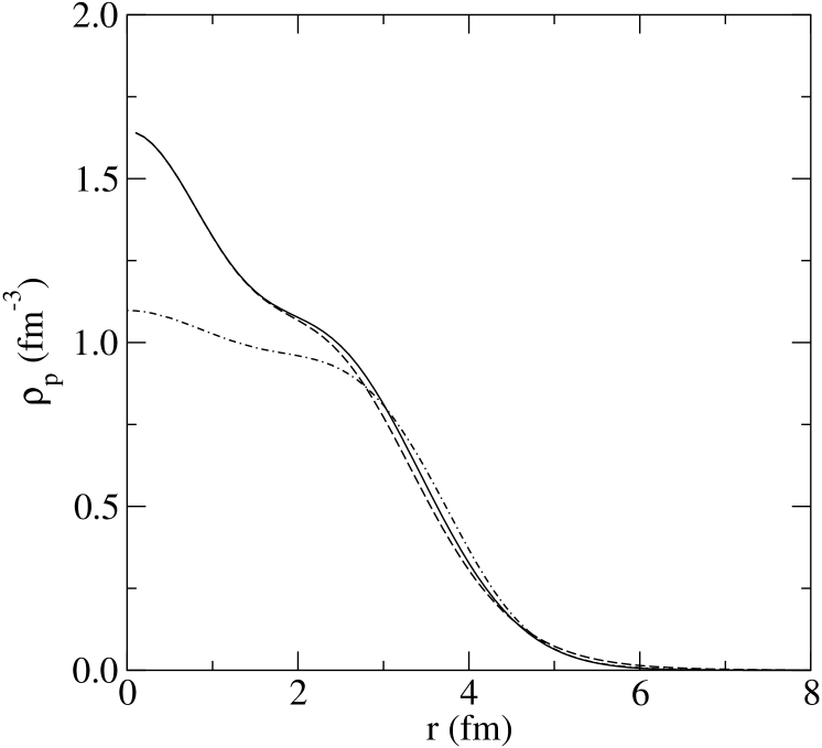
Figure 12: The proton matter densities in ⁴⁰Ca given by the HO (dashed), the $m=8$ harmonic mean transformations (solid), and the SHF/SKX (dot-dashed) models.

In this case, the LST density is similar to that of the input shell model function; the surface being slightly extended. Both differ most noticeably from the SHF/SKX in the nuclear interior, and the SHF/SKX model density extends further still. But the large interior difference is not very important in the analyses we make as the volume integral contribution of that region is not large. In use of these wave functions to define optical potentials that volume integration contribution as well as the inherent absorption makes the region inside about 2 fm of small import for most scattering. It is the surface differences that one may expect to most influence results.

V Applications in scattering analyses

The harmonic mean LST wave functions determined from the $m=8$ formulation have been used as input into calculations of elastic scattering of the radioactive ions from hydrogen targets as well as of proton scattering from the stable nucleus ⁴⁰Ca. A modified version of the code DWBA98 Raynal (1998) has been used with appropriate effective $NN$ interactions for each energy considered with OBDME obtained for each nucleus as outlined earlier.

V.1 Scattering of ^6,8He and ¹¹Li

Elastic scattering of $24.5A$, $40.9A$ and $70.5A$ MeV ⁶He ions from hydrogen has been measured and analyzed Lagoyannis et al. (2001); Stepantsov et al. (2002); Korsheninnikov et al. (1993, 1997) revealing that this nucleus has a neutron matter distribution more consistent with a neutron halo than a neutron skin, as the naive shell model predicts. That was definitely the case considering the $24.5A$ MeV elastic scattering data. At $40.9A$ MeV, the DWA analysis of the scattering data for excitation of the $2^{+}_{1}$ state was the prime evidence for a halo. The $70.5A$ MeV elastic scattering data do not extend to large enough momentum transfer to distinguish the halo aspect clearly but we include it to show a set of data for which the method used to predict the cross sections is reliable. In those previous studies the neutron halo was artificially created by choosing weak binding for the $0p$ neutron orbits and using WS potentials to define the radial wave functions.

Differential cross sections for the scattering of $24.5A$, $40.9A$, and $70.5A$ MeV ⁶He ions from Hydrogen, as obtained using the $m=8$ LST on the HO functions with binding energies listed in Table 1, are shown by the solid curves in Fig. 13. Therein the data are shown by the open circles

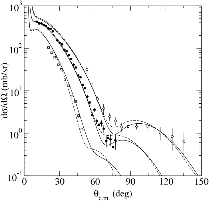
Figure 13: The elastic scattering differential cross sections for $24.5A$, $40.9A$, and $70.5A$ MeV ⁶He ions from hydrogen. For each energy the LST ($m=8$) result is portrayed by the solid line while that result obtained from the WS SP wave functions is given by the dashed line.

($24.5A$ MeV), the filled circles ($40.9A$ MeV), and the open squares ($70.5A$ MeV). The previous halo results Lagoyannis et al. (2001); Stepantsov et al. (2002); Karataglidis et al. (2000) are shown by the dashed curves for comparison. Our transformed wave functions serve to correct the description of these data as does the more ad hoc selection of disparate WS functions Lagoyannis et al. (2001) for the occupied orbits by being distinctively different from those obtained when no extension to neutron matter was considered. The data at $24.5A$ and $40.9A$ MeV extend beyond the first minimum into the region where one may distinguish between the halo and non-halo regions Lagoyannis et al. (2001); Stepantsov et al. (2002). Both the WS and LST results agree well with those data, indicating that our modifications to the HO wave functions with the LST make the necessary corrections to explain the data. This is consistent with our results concerning both the rms radius and the reaction cross section. Both the WS and LST results agree equally well with the available data at $70.5A$ MeV.

Previously the scattering data analyses confirmed what had been expected from heavy ion collision studies that ⁸He has a neutron skin but not the extended distribution one now identifies as a halo. The appropriate LST for SP wave functions for this nucleus, again predicated upon an oscillator length of 1.6 fm, retains a skin attribute and results in the differential cross section for $72A$ MeV ⁸He ions from hydrogen shown in Fig. 14 by the solid line. The data were taken from Refs. Korsheninnikov et al. (1993, 1997) and the dashed curve is the result that was obtained previously Karataglidis et al. (2000) when those SP wave functions were taken as the earlier published WS set.

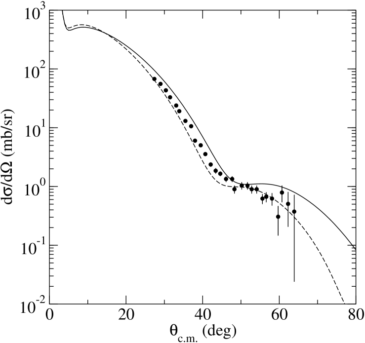
Figure 14: The elastic scattering differential cross sections for $72A$ MeV ⁸He ions from hydrogen. The results of the calculations made using the LST ($m=8$) and WS sets of SP wave functions are displayed by the solid and dashed lines, respectively.

Both results do well in describing the available data.

The nucleus ¹¹Li is known to have an extended neutron (halo) density. That was confirmed from the analyses of elastic scattering of ¹¹Li ions from hydrogen Karataglidis et al. (2000) and those results are displayed again in Fig. 15 along with our new results obtained by using the same approach, with the same effective force, but with the transformed HO wave functions.

Figure 15: Data from the elastic scattering of $62A$ MeV ¹¹Li ions from hydrogen compared to the predictions made using the basic shell model wave functions (dotted curve), with the WS (halo) functions (dot-dashed curve), and with the $m=4$ (dashed curve) and $m=8$ (solid curve) harmonic mean transformed wave functions.

As noted previously the difference between using WS wave functions with binding energies chosen to obtain a halo in the neutron matter density in this nucleus and those wave functions that set it to have only a skin, is striking. Only with the halo specification does a good prediction of the data result. That is true also for the transformed HO functions, with the $m=4$ LST providing excellent reproduction of the data. While the results obtained from the LST transformation with $m=8$ provides good reproduction up to $50^{\circ}$ it overestimates the larger angle data.

V.2 Scattering from ⁴⁰Ca

Finally we consider the use of the LST functions for ⁴⁰Ca in generating optical potentials. With those functions we have made predictions of the elastic scattering of 65 and of 200 MeV protons. Such data were analyzed recently Karataglidis et al. (2002) and very good differential cross-section results were obtained for both energies; especially when the SHF/SKX model wave functions were used. Those SHF/SKX results are shown again in Fig. 16 for both energies by the dot-dashed curves.

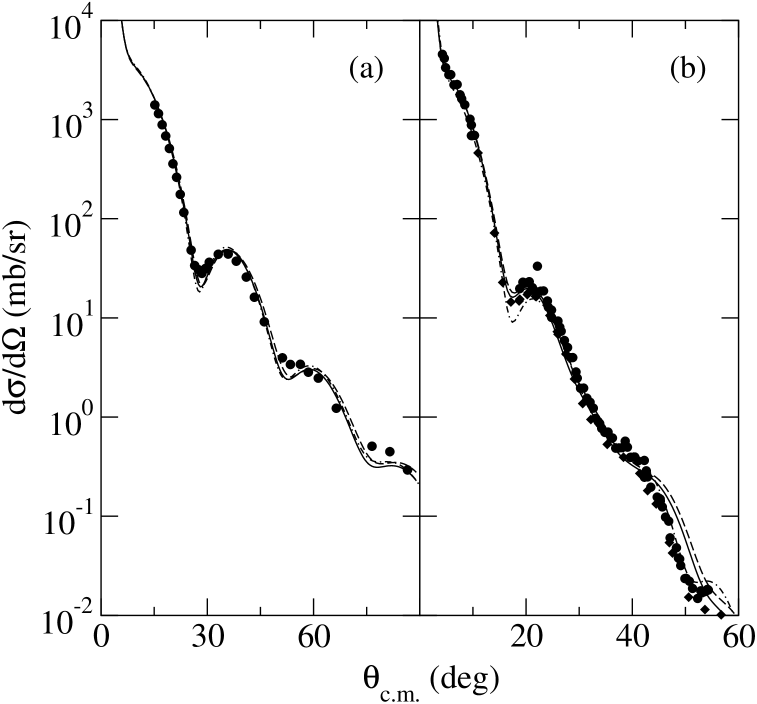
Figure 16: Data from the elastic scattering of 65 MeV (a) and of 200 MeV (b) protons from ⁴⁰Ca compared with predictions made using the basic shell model wave functions (dashed curve), with the SHF/SKX functions (dot-dashed curve), and with the $m=8$ (solid curve) harmonic mean transformed wave functions.

The shell model ($b=1.9$ fm) results are those portrayed by the dashed curves while the LST function results are given by the solid curves. Note that the shell model results are varied from those found earlier Karataglidis et al. (2002); the result of our changing the oscillator length slightly from that defined by Karataglidis and Chadwick Karataglidis et al. (2002). The adjustment was made specifically to obtain the best possible agreement with the data from the shell model. That allows for the most sensitivity to changes wrought by the LST. The changes are slight but they in fact improve agreement with observation. But neither our shell model or the LST built from it give results as good as the SHF/SKX model of structure. Clearly while the LST may give more reasonable matter profiles to a model of the ground state structure, it is not a panacea for a too limited initial guess. Use of the LST approach with “best model” structures of nuclei are in train.

VI Summary and conclusions

Using local scale transformations of the radial coordinate within the Gaussian wave functions assumed to describe bound nucleons in shell model studies, gives new descriptions of those nucleon functions that have exponentially decreasing forms consistent with selected values for their binding energies. Orthonormality of those transformed wave functions can be assured quite easily. Herein we have considered an harmonic mean form of local scale transforms.

As an empirical example, the harmonic mean LST (of rank 8) was used to specify a set of single nucleon bound state orbitals for use in defining optical potentials to describe the elastic scattering of light mass radioactive ions (^6,8He and ¹¹Li specifically) from hydrogen as well as for the scattering of protons from the stable nucleus ⁴⁰Ca. Those optical potentials were formed by $g$-folding: folding of complex effective $NN$ interactions in which medium modification due to both Pauli blocking and a background mean field had been taken into consideration with the LST generated single nucleon wave functions weighted by the OBDME given by shell model calculations. The resultant nonlocality of those optical potentials was treated exactly. The results for the elastic scattering of $24.5A$, $40.9A$ and of $70.5$ MeV ⁶He ions from hydrogen agreed well with both the data and previous calculations in which WS wave functions were used. With both the ad hoc WS and the LST formed wave functions, ⁶He has a neutron distribution so extended from that associated with the shell model (Gaussian functions) as to be consistent with a halo. Notably, the WS and LST densities are in good agreement. However, it is also of note that in order to obtain such agreement in the densities, the chosen sets of SP binding energies need not be the same, as the underlying potentials (WS and HO) are different. For ⁸He, the LST (and WS) functions involved also give good results in comparison with scattering data taken at $72A$ MeV. In this case the neutron extension is not as large as that for ⁶He resulting in this nucleus defined to have a neutron skin rather than a halo. Yet with both nuclei we find an extension of the proton density beyond the HO result. That dilution of the proton density is influenced by the extension of the neutron density, as expected for neutron-rich nuclei. Also, a good result in comparison to data is obtained when cross sections for the elastic scattering of $62A$ MeV ¹¹Li ions from hydrogen were considered. The LST wave functions again extend the neutron distribution for this nucleus so much that we deem it to be a neutron halo. In this case it was due mainly to the neutron occupancy of the $0p_{1/2}$ and $1s_{1/2}$ orbits and we took care to ensure that $1s_{1/2}$ orbit was orthogonal to the $0s_{1/2}$. In this case we noted that the rank of the harmonic mean has some import regarding the quality of the agreement of the results with data.

Finally, as a check case, we found that using the LST to vary the shell model single nucleon wave functions for a stable nucleus case did not vitiate the good results previously found for scattering cross sections with potentials formed by $g$-folding with the shell model wave functions themselves. The cross sections from 65 and 200 MeV protons elastically scattered from ⁴⁰Ca were considered. ⁴⁰Ca was considered also as there exist SHF wave functions to describe its ground state and whose use in $g$-folding gave potentials and scattering results also in very good agreement with the data. However, the densities formed by the shell and the SHF models are different, most noticeably in the central region and also in the surface. The LST modifications vary the shell model density most through the surface region and therefore does not give changes inside the nucleus to match the SHF results. Of course, as the SHF wave functions need not have appropriate exponential tails either, it is feasible to apply the LST scheme to those. That is under investigation.