Anisotropic multi–gap superfluid states
in nuclear matter

Abstract

It is shown that under changing density or temperature a nucleon Fermi superfluid can undergo a phase transition to an anisotropic superfluid state, characterized by nonvanishing gaps in pairing channels with singlet–singlet (SS) and triplet-singlet (TS) pairing of nucleons (in spin and isospin spaces). In the SS pairing channel nucleons are paired with nonzero orbital angular momentum. Such two–gap states can arise as a result of branching from the one-gap solution of the self-consistent equations, describing SS or TS pairing of nucleons, that depends on the relationship between SS and TS coupling constants at the branching point. The density/temperature dependence of the order parameters and the critical temperature for transition to the anisotropic two–gap state are determined in a model with the SkP effective interaction. It is shown that the anisotropic SS–TS superfluid phase corresponds to a metastable state in nuclear matter.

I Introduction

It is known that at sufficiently low temperatures a nucleon Fermi system becomes unstable with respect to formation of Cooper pairs due to the attractive component of the nucleon–nucleon (NN) potential. Basically in early articles on superfluidity isovector pairing of the same nucleons in nuclei and nuclear matter BM ; RS was studied. Later it was realized that isoscalar neutron–proton pairing plays an essential role in the description of superfluidity of finite nuclei with $N\simeq Z$ (see Refs. G ; RSSL and references therein) and nearly symmetric nuclear matter AFRS –SAL . Possible coexistence of isoscalar and isovector nucleon pairing in finite nuclei was studied in Ref. G1 . In addition to isovector pairing, isoscalar pairing modes have been investigated to explain the excitation energies in $N=Z$ nuclei SW . As was shown in Ref. AIP2 , at low densities of nuclear matter the coupling between isospin $T=0$ and $T=1$ pairing channels may be of importance, leading to the emergence of multi–gap superfluid states with nonvanishing gaps in both pairing channels. In Refs. AIP2 ; AAI the case of a multi–gap condensate was considered, when the energy gaps in ${}^{1}S_{0}$ and ${}^{3}S_{1}$ pairing channels are nonzero. For such a condensate the orbital angular momentum $L$ of a pair is equal to zero and, hence, the order parameters in both pairing channels are isotropic functions of the momentum. However, we can consider another possibility, when the pairing of nucleons in one (or both) pairing channels occurs in a state with nonzero orbital angular momentum. In this case an anisotropic multi–gap condensate will be realized, where the order parameter(s) will depend not only on the absolute value of momentum, but also on its direction. Further we will consider an isoscalar multi–gap superfluid state, corresponding to a superposition of pair states with spin $S=0$ and $S=1$. According to the Pauli principle, the orbital angular momentum in the first pairing channel ($S=0,T=0$) is odd and in the second one ($S=1,T=0$) it is even. Hence, such a multi–gap condensate will necessarily be anisotropic. Our main purpose will be the clarification of a mechanism for the appearance of anisotropic multi–gap superfluid states, finding the corresponding critical temperature and comparing the free energies for different superfluid phases. As a theoretical framework, we use the Fermi–liquid (FL) approach  AKP , in which normal and anomalous FL interaction amplitudes are treated on an equal footing. As a NN interaction we choose the density dependent Skyrme effective forces, used earlier in a number of contexts for calculations in finite nuclei DFT ; RDN and infinite nuclear matter SYK –AIPY . In specific calculations we use the SkP potential DFT , for which the strongest interaction in the state of a Cooper pair with nonzero orbital angular momentum is realized in the pairing channel $S=0,T=0$, and in the state with $L=0$ it is in the channel $S=1,T=0$.

II Basic Equations

Superfluid states of nuclear matter are described by the normal $f_{\kappa_{1}\kappa_{2}}=\mbox{Tr}\,\varrho a^{+}_{\kappa_{2}}a_{\kappa_{1}}$ and anomalous $g_{\kappa_{1}\kappa_{2}}=\mbox{Tr}\,\varrho a_{\kappa_{2}}a_{\kappa_{1}}$ distribution functions of nucleons ($\kappa\equiv({\bf{p}},\sigma,\tau)$, ${\bf p}$ is momentum, $\sigma(\tau)$ is the projection of spin (isospin) on the third axis, $\varrho$ is the density matrix of the system). The energy of the system is specified as a functional of the distribution functions $f$ and $g$, $E=E(f,g)$. It determines the quasiparticle energy $\varepsilon$ and the matrix order parameter $\Delta$ of the system

$$\varepsilon_{\kappa_{1}\kappa_{2}}=\frac{\partial{E}}{\partial{f_{\kappa_{2}\kappa_{1}}}},\quad\Delta_{\kappa_{1}\kappa_{2}}=2\frac{\partial{E}}{\partial{g_{\kappa_{2}\kappa_{1}}^{+}}}\,\,.$$ (1)

The self-consistent matrix equation for determining the distribution functions $f$ and $g$ follows from the minimum condition of the thermodynamic potential AKP and is

$$\hat{f}=\left\{\mbox{exp}(Y_{0}\hat{\varepsilon}+\hat{Y}_{4})+1\right\}^{-1}\equiv\left\{\mbox{exp}(Y_{0}\hat{\xi})+1\right\}^{-1},$$ (2)

$$\hat{f}=\left(\begin{array}[]{cc}f&g\\ g^{+}&1-f^{\mbox{\small T}}\end{array}\right),\;\hat{\varepsilon}=\left(\begin{array}[]{cc}\varepsilon&\Delta\\ \Delta^{+}&-\varepsilon^{\mbox{\small T}}\end{array}\right),\;$$

$$\hat{Y}_{4}=\left(\begin{array}[]{cc}Y_{4}&0\\ 0&-Y_{4}\end{array}\right)\,\,.$$

Here the quantities $\varepsilon,\Delta,Y_{4}$ are, in turn, matrices in the space of the $\kappa$ variables, with $Y_{4\kappa_{1}\kappa_{2}}=Y_{4\tau_{1}}\delta_{\kappa_{1}\kappa_{2}}$ $(\tau_{1}=p,n)$, $Y_{0}=1/T,\ Y_{4p}=-\mu_{p}/T$ and $Y_{4n}=-\mu_{n}/T$ are the Lagrange multipliers, $\mu_{p}$ and $\mu_{n}$ are the chemical potentials for protons and neutrons, $T$ is the temperature. We shall study two–gap superfluid states in symmetric nuclear matter, corresponding to a superposition of pair states with total spin $S$ and isospin $T$: $S=0$, $T=0$ (singlet–singlet (SS) pairing in spin and isospin spaces) and $S=1,T=0$ (triplet–singlet (TS) pairing) with the projections $S_{z}=T_{z}=0$ (SS–TS states). In this case the normal $f$ and anomalous $g$ distribution functions read AIP

$$f({\bf p}) =f_{00}({\bf p})\sigma_{0}\tau_{0},$$ (3)

$$g({\bf p}) =g_{00}({\bf p})\sigma_{2}\tau_{2}+g_{30}({\bf p})\sigma_{3}\sigma_{2}\tau_{2},$$

where $\sigma_{i}$ and $\tau_{k}$ are the Pauli matrices in spin and isospin spaces, respectively. The components of the anomalous distribution function in Eq. (3) possess different symmetry properties,

$$g_{00}(-{\bf p})=-g_{00}({\bf p}),\;g_{30}(-{\bf p})=g_{30}({\bf p}),$$ (4)

and, hence, considering this, the multi–gap condensate will be anisotropic. For the energy functional, which is invariant with respect to rotations in spin and isospin spaces, the structure of the single particle energy and the order parameter is similar to that of the distribution functions $f,g$:

$$\varepsilon({\bf p}) =\varepsilon_{00}({\bf p})\sigma_{0}\tau_{0},$$ (5)

$$\Delta({\bf p}) =\Delta_{00}({\bf p})\sigma_{2}\tau_{2}+\Delta_{30}({\bf p})\sigma_{3}\sigma_{2}\tau_{2},$$

where

$$\Delta_{00}(-{\bf p})=-\Delta_{00}({\bf p}),\;\Delta_{30}(-{\bf p})=\Delta_{30}({\bf p}).$$ (6)

Using the procedure of block diagonalization AKP , one can evidently express the distribution functions $f_{00},g_{00},g_{30}$ in terms of the quantities $\varepsilon$ and $\Delta$:

$$f_{00} =\frac{1}{2}\left[1-\frac{\xi}{2E_{+}}(1-2n_{+})-\frac{\xi}{2E_{-}}(1-2n_{-})\right],$$ (7)

$$g_{00} =-\frac{\Delta_{+}}{4E_{+}}(1-2n_{+})-\frac{\Delta_{-}}{4E_{-}}(1-2n_{-}),$$ (8)

$$g_{30} =-\frac{\Delta_{+}}{4E_{+}}(1-2n_{+})+\frac{\Delta_{-}}{4E_{-}}(1-2n_{-}).$$ (9)

Here

$$E_{\pm}=\sqrt{\xi^{2}+|\Delta_{\pm}|^{2}},\quad\Delta_{\pm}=\Delta_{00}\pm\Delta_{30},$$

$$\xi({\bf p})=\varepsilon_{00}({\bf p})-\mu_{0},\;n_{\pm}=\{\exp(Y_{0}E_{\pm})+1\}^{-1},$$

$\mu_{0}$ is the chemical potential, which should be determined from the normalization condition

$$\frac{4}{\cal V}\sum_{\bf p}f_{00}({\bf p})=\varrho,$$ (10)

$\varrho$ is density of symmetric nuclear matter. As follows from Eqs. (7)–(9), the nucleon superfluid is characterized by two types of fermion excitations with gaps $\Delta_{\pm}$ in the spectrum. In this case the spectrum is two–fold split due to coupling of SS and TS pairing channels ($\Delta_{00}\not=0,\Delta_{30}\not=0$).

To obtain the self–consistent equations for the quantities $\Delta$ and $\xi$, it is necessary to specify the energy functional of the system, which we write in the form

$$E(f,g)=E_{0}(f)+E_{int}(f)+E_{int}(g),$$ (11)

$${E}_{0}(f) =4\sum\limits_{\bf p}\varepsilon_{0}({\bf p})f_{00}({\bf p}),\;{E}_{int}(f)=2\sum\limits_{\bf p}\tilde{\varepsilon}_{00}({\bf p})f_{00}({\bf p}),$$

$$\varepsilon_{0}({\bf p}) =\frac{{\bf p}^{\,2}}{2m_{0}},\,\tilde{\varepsilon}_{00}({\bf p})=\frac{1}{2\cal V}\sum_{\bf q}U_{0}({\bf k})f_{00}({\bf q}),\,{\bf k}=\frac{{\bf p}-{\bf q}}{2},$$

$${E}_{int}(g) = \frac{2}{\cal V}\sum\limits_{{\bf p},{\bf q}}\Bigl{(}g_{00}^{*}({\bf p})V_{0}({\bf p},{\bf q})g_{00}({\bf q})$$

$$+ g_{30}^{*}({\bf p})V_{1}({\bf p},{\bf q})g_{30}({\bf q})\Bigr{)}.$$

Here $m_{0}$ is the bare mass of a nucleon, $U_{0}({\bf k})$ is the normal FL amplitude, $V_{0}({\bf p},{\bf q}),V_{1}({\bf p},{\bf q})$ are the anomalous FL amplitudes, describing interactions in the SS and TS pairing channels, respectively. With allowance for Eqs. (1), (11), we obtain self–consistent equations in the form

$$\xi({\bf p}) =\varepsilon_{0}({\bf p})-\mu_{0}+\tilde{\varepsilon}_{00}({\bf p}),\;$$ (12)

$$\Delta_{00}({\bf p}) =\frac{1}{\cal V}\sum_{\bf q}V_{0}({\bf p},{\bf q})g_{00}({\bf q}),\;$$ (13)

$$\Delta_{30}(\bf p) =\frac{1}{\cal V}\sum_{\bf q}V_{1}({\bf p},{\bf q})g_{30}({\bf q}).$$ (14)

Taking into account Eqs. (8), (9), we obtain equations for the energy gaps $\Delta_{00},\Delta_{30}$

$$\Delta_{00}({\bf p})=-\frac{1}{4\cal{V}}\sum\limits_{\bf q}V_{0}({\bf p},{\bf q})$$ (15)

$$\times\left\{\frac{\Delta_{+}({\bf q})}{E_{+}({\bf q)}}\tanh\frac{E_{+}({\bf q})}{2T}+\frac{\Delta_{-}({\bf q})}{E_{-}({\bf q)}}\tanh\frac{E_{-}({\bf q})}{2T}\right\},$$

$$\Delta_{30}({\bf p})=-\frac{1}{4\cal{V}}\sum\limits_{\bf q}V_{1}({\bf p},{\bf q})$$ (16)

$$\times\left\{\frac{\Delta_{+}({\bf q})}{E_{+}({\bf q)}}\tanh\frac{E_{+}({\bf q})}{2T}-\frac{\Delta_{-}({\bf q})}{E_{-}({\bf q)}}\tanh\frac{E_{-}({\bf q})}{2T}\right\}.$$

Eqs. (12), (15), (16) describe two–gap superfluid states of symmetric nuclear matter and contain one–gap solutions with $\Delta_{00}\not=0,\Delta_{30}\equiv 0$ (SS pairing) and $\Delta_{00}\equiv 0,\Delta_{30}\not=0$ (TS pairing) as some particular cases.

To obtain numerical results we will use the Skyrme effective interaction, for which the normal and anomalous FL amplitudes read AIP

$$U_{0}({\bf k}) =6t_{0}+t_{3}\varrho^{\beta}$$ (17)

$$\quad+\frac{2}{\hbar^{2}}[3t_{1}+t_{2}(5+4x_{2})]{\bf k}^{2},$$

$$V_{0}({\bf p},{\bf q}) =\frac{t_{2}}{\hbar^{2}}(1-x_{2}){\bf p}{\bf q}\equiv V_{0}(p,q){\bf p}^{0}{\bf q}^{0},$$ (18)

$$V_{1}({\bf p},{\bf q}) =t_{0}(1+x_{0})+\frac{1}{6}t_{3}\varrho^{\beta}(1+x_{3})$$ (19)

$$\quad+\frac{1}{2\hbar^{2}}t_{1}(1+x_{1})({\bf p}^{2}+{\bf q}^{2}),$$

where $t_{i},x_{i},\beta$ are phenomenological constants, characterizing the given parametrization of Skyrme forces. (We shall use the SkP DFT potential.) According to Eqs. (18), (19), pairing in the SS channel occurs with orbital angular momentum $L=1$ and in the TS channel with $L=0$. Note that in the case of the effective Skyrme interaction the normal FL amplitude $U_{0}$ is quadratic in momentum and hence describes a renormalization of free nucleon mass and chemical potential. The expression for the quantity $\xi$, given by Eq. (12), with regard for the explicit form of the amplitude $U_{0}$, reads

$$\xi=\frac{p^{2}}{2m}-\mu,$$

where the effective nucleon mass $m$ is defined by the formula

$$\frac{\hbar^{2}}{2m}=\frac{\hbar^{2}}{2m_{0}}+\frac{\varrho}{16}[3t_{1}+t_{2}(5+4x_{2})]$$

and the effective chemical potential $\mu$ should be determined from Eq. (10).

III Order parameters at zero temperature

Let us consider the case of zero temperature. We shall analyze Eqs. (15),(16), using the simplifying assumption, that FL amplitudes $V_{0},V_{1}$ are nonzero only in a narrow layer near the Fermi surface: $|\xi|\leq\theta,\,\theta\ll\varepsilon_{F}$ (we set $\theta=0.1\varepsilon_{F}$). Then the TS energy gap represents some constant quantity $\Delta_{30}\equiv\Delta_{30}(p=p_{F})$, while the SS energy gap is angular dependent, $\Delta_{00}=\Delta{\bf p}^{0}{\bf n}$, ${\bf n}$ being an arbitrary real unit vector. In addition, we shall neglect the influence of the finite size of the gaps on the chemical potential $\mu$ and set $\mu=\frac{\hbar^{2}k_{F}^{2}}{2m}$, $k_{F}=\left(\frac{3\pi^{2}\varrho}{2}\right)^{1/3}$. As a result of these assumptions, we arrive at equations for determining the quantities $\Delta,\Delta_{30}$:

$$\Delta =\frac{g_{0}}{2}\int_{0}^{\theta}\,d\xi\int_{0}^{1}\,dxx\Bigl{(}\frac{\Delta x+\Delta_{30}}{E_{+}}+\frac{\Delta x-\Delta_{30}}{E_{-}}\Bigr{)},$$ (20)

$$\Delta_{30} =\frac{g_{1}}{2}\int_{0}^{\theta}\,d\xi\int_{0}^{1}\,dx\Bigl{(}\frac{\Delta x+\Delta_{30}}{E_{+}}-\frac{\Delta x-\Delta_{30}}{E_{-}}\Bigr{)},$$ (21)

where

$$E_{\pm}=\sqrt{\xi^{2}+|\Delta x\pm\Delta_{30}|^{2}},\quad g_{0,1}=-\nu_{F}V_{0,1}(p_{F},p_{F})$$

and $\nu_{F}=\frac{mp_{F}}{2\pi^{2}\hbar^{3}}$ is the density of states at the Fermi surface for a nucleon with the given spin and isospin projections. Our main goal is to find two–gap solutions with $\Delta\not=0,\Delta_{30}\not=0$ and to clarify the mechanism of their appearance. To give some analytical consideration, we will assume that the conditions $\Delta,\Delta_{30}\ll\theta$ are fulfilled (logarithmic approximation). As will become apparent, this approximation works quite well just in the density region where the two–gap solutions exist. Introducing the ratio of the energy gaps $\alpha=\Delta_{30}/\Delta$ and performing integration in Eqs. (20),(21) in the logarithmic approximation, we arrive at equations for the quantities $\alpha$ and $\Delta$:

$$\frac{1}{g_{1}} =\frac{1}{2}+\ln\frac{2\theta}{|\Delta|}-\frac{1}{2}\ln|\alpha^{2}-1|-\frac{1}{4}(\alpha+\frac{1}{\alpha})\ln\left|\frac{\alpha+1}{\alpha-1}\right|,$$

$$\frac{3}{g_{0}} =\frac{1}{3}+\ln\frac{2\theta}{|\Delta|}-\frac{1}{2}\ln|\alpha^{2}-1|$$ (22)

$$\quad+\frac{\alpha}{4}(\alpha^{2}-3)\ln\left|\frac{\alpha+1}{\alpha-1}\right|-\frac{\alpha^{2}}{2}\,\,.$$

Excluding $\Delta$ from Eqs. (22), we obtain the equation

$$\frac{1}{g_{1}}-\frac{3}{g_{0}}=\varphi(\alpha),\;\varphi(\alpha)\equiv\frac{1}{2}(\alpha^{2}+\frac{1}{3})-\frac{(\alpha^{2}-1)^{2}}{4\alpha}\ln\left|\frac{1+\alpha}{1-\alpha}\right|$$ (23)

Since $\varphi_{min}=\varphi(0)=-1/3$ (the point $\alpha=0$ is the point of removable discontinuity) and $\varphi_{max}=\varphi(\pm\infty)=1$, then Eq. (23) has a solution for $\alpha$, if the coupling constants $g_{0}$ and $g_{1}$ satisfy the inequalities

$$-\frac{1}{3}<\frac{1}{g_{1}}-\frac{3}{g_{0}}<1.$$ (24)

These restrictions have to be fulfilled in the logarithmic approximation for the existence of the SS–TS mixed state. The sense of the restrictions (24) on SS and TS coupling constants is that the quantities $g_{1}$ and $g_{0}/3$ must be of the same order of magnitude. Clearly, similar restrictions exist in a general case, when the conditions of the logarithmic approximation are not fulfilled. Note that the constraints (24) are more strict than the corresponding ones for the existence of a TS–ST mixed state  AIP2  :$-1<1/g_{1}-1/g_{2}<1,\ g_{2}=-\nu_{F}V_{2}(p_{F},p_{F})$ (the constants $g_{1},g_{2}$, determined here, are four times as large as those in Ref. AIP2 ).

The results of a numerical determination of the energy gaps $\Delta(\varrho),\Delta_{30}(\varrho)$ as functions of density from Eqs. (20), (21) are presented in Fig. 1, where the part of the phase diagram corresponding to the mixed SS–TS states is shown.

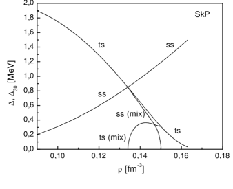
Figure 1: Order parameters $\Delta,\Delta_{30}$ vs. density at zero temperature for SkP force; $ss$(mix) and $ts$(mix) are notations for the dependencies of the energy gaps $\Delta$ and $\Delta_{30}$ in the mixed SS–TS solution.

One can see that SS–TS solutions exist in the finite density region $\varrho_{1}<\varrho<\varrho_{2}$. In the left critical point two–gap solutions appear as a result of branching from a one–gap SS solution (at the branching point $\Delta_{30}(\varrho_{1})=0,\,\,\Delta(\varrho_{1})=\Delta^{{ss}}(\varrho_{1})$, $\Delta^{{ss}}$ being a one–gap SS solution). At $\varrho=\varrho_{1}$ the coupling constants are related by the formula

$$\frac{1}{g_{1}(\varrho_{1})}-\frac{3}{g_{0}(\varrho_{1})}=-\frac{1}{3}.$$ (25)

In the logarithmic approximation the one–gap SS and TS order parameters have the form

$$\Delta^{ss}=2\theta\exp\Bigl{(}-\frac{3}{g_{0}}+\frac{1}{3}\Bigr{)},\;\Delta_{30}^{ts}=2\theta\exp\Bigl{(}-\frac{1}{g_{1}}\Bigr{)}.$$

From here and Eq. (25) it follows that at zero temperature at the left branching point the energy gaps in the SS and TS pairing channels are equal, $\Delta^{ss}(\varrho_{1})=\Delta^{ts}(\varrho_{1})$. This peculiarity is preserved for finite temperatures, as will be seen in Section IV.

In the right critical point the two–gap solutions branch off from a one–gap TS solution (at the branching point $\Delta(\varrho_{2})=0,\Delta_{30}(\varrho_{2})=\Delta_{30}^{ts}(\varrho_{2})$). At $\varrho=\varrho_{2}$

$$\frac{1}{g_{1}(\varrho_{2})}-\frac{3}{g_{0}(\varrho_{2})}=1.$$ (26)

Note that the conditions of the logarithmic approximation, $\Delta\ll\theta,\Delta_{30}\ll\theta$, are fulfilled quite satisfactorily in the density domain where the two–gap solutions exist: the maximum value of the ratios $\Delta/\theta,\Delta_{30}/\theta$ does not exceed $0.26$.

From Fig. 1 it is seen that SS–TS mixed states exist in a density interval that is much closer to nuclear matter saturation density than that for TS–ST multi–gap states AIP2 , which exist in the region $\varrho<\varrho^{\prime}$, where $\varrho^{\prime}\approx 0.05\div 0.06\ \mbox{fm}^{-3}$. Hence, there is no competition between SS–TS and TS–ST superfluid states, which exist in quite different density domains.

IV Critical temperature, Order parameters at nonzero temperature

The analysis given in the previous section relates to the case of zero temperature. It is clear that if SS–TS states exist at T=0, then such states appear first at some critical temperature. To determine the critical temperature we use the following considerations. Obviously, SS–TS solutions arise as a result of branching from SS or TS one–gap solutions of Eqs. (15),(16). If branching occurs from a TS solution then at the critical point $\Delta(T_{c})=0,\Delta_{30}(T_{c})=\Delta_{30}^{ts}(T_{c})$. Considering the limit $\Delta\rightarrow 0$ in Eqs. (15),(16), we obtain equations for determining $T_{c}$

$$1 =g_{1}\int_{0}^{\theta}\frac{d\xi}{E}\tanh\frac{E}{2T_{c}},\quad E=\sqrt{\xi^{2}+\Delta_{30}^{2}},$$ (27)

$$1 =\frac{g_{0}}{3}\int_{0}^{\theta}d\xi\,\Bigl{\{}\frac{\xi^{2}}{E^{3}}\tanh\frac{E}{2T_{c}}+\frac{\Delta_{30}^{2}}{2E^{2}T_{c}}\frac{1}{\cosh^{2}\frac{E}{2T_{c}}}\Bigr{\}}.$$ (28)

The first of these equations determines the temperature behavior of TS energy gap, the second one determines the critical temperature $T_{c}$ at which the mixed SS–TS solution branches from the one–gap TS solution. If SS–TS states appear from a SS solution, then $\Delta_{30}(T_{c})=0,\Delta(T_{c})=\Delta^{ss}(T_{c})$. Considering the limit $\Delta_{30}\rightarrow 0$ in Eqs. (15),(16), we obtain

$$1 =g_{0}\int_{0}^{\theta}d\xi\,\int_{0}^{1}dx\,\frac{x^{2}}{E}\tanh\frac{E}{2T_{c}},\;E=\sqrt{\xi^{2}+\Delta^{2}x^{2}},$$ (29)

$$1 =g_{1}\int_{0}^{\theta}d\xi\,\int_{0}^{1}dx\Bigl{\{}\frac{\xi^{2}}{E^{3}}\tanh\frac{E}{2T_{c}}$$

$$\quad+\frac{\Delta^{2}x^{2}}{2E^{2}T_{c}}\frac{1}{\cosh^{2}\frac{E}{2T_{c}}}\Bigr{\}}\,\,.$$ (30)

Here the first equation determines the temperature behavior of the SS energy gap, the second one determines the critical temperature $T_{c}$ at which the mixed SS–TS solution branches from the one–gap SS solution.

The results of a numerical solution of Eqs. (27),(28) and Eqs. (29),(30) are presented in Fig. 2.

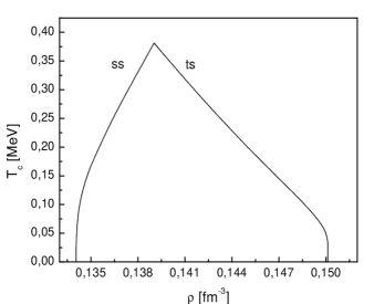
Figure 2: Critical temperature of SS–TS superfluid state vs. density for SkP force; notations $ss$ and $ts$ correspond to branching of SS–TS solutions from SS and TS one–gap solutions, respectively.

One can see that the curve $T_{c}(\varrho)$ consists of two branches. The left branch corresponds to the appearance at a critical temperature $T_{c}$ of a SS–TS solution from the SS one–gap solution, the right one corresponds to the appearance of a SS–TS solution from the TS one–gap solution. The maximum value of $T_{c}$ is approximately equal to $0.38$ MeV at density $\varrho_{m}\approx 0.139\;\mbox{fm}^{-3}$. In the limit $T_{c}\rightarrow 0$, from Eqs. (27),(28), we obtain Eq. (26) for the right critical point $\varrho=\varrho_{2}$ ($\varrho_{2}\approx 0.15\;\mbox{fm}^{-3}$) and from Eqs. (29),(30) we obtain Eq. (25) for the left critical point $\varrho=\varrho_{1}$ ($\varrho_{1}\approx 0.134\;\mbox{fm}^{-3}$). Thus, in the density interval $(\varrho_{1},\varrho_{m})$ SS–TS solutions appear as a result of a phase transition in temperature from a one–gap SS solution, and in the interval $(\varrho_{m},\varrho_{2})$ they appear from a one–gap TS solution. If $\varrho_{1}<\varrho<\varrho_{m}$, the coupling constants satisfy the inequality $g_{1}>g_{0}/3$, and for $\varrho_{m}<\varrho<\varrho_{2}$ it is $g_{1}<g_{0}/3$.

To determine the temperature behavior of the order parameters, one should consider Eqs. (15), (16). According to our analysis we can consider two possibilities, when branching occurs at density $\varrho$ such that (1) $\varrho_{1}<\varrho<\varrho_{m}$ and (2) $\varrho_{m}<\varrho<\varrho_{2}$. The results of numerical calculations are shown in Fig. 3.

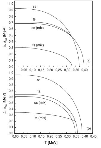
Figure 3: Order parameters $\Delta,\Delta_{30}$ vs. temperature at density (a) $\varrho=0.138\ \mbox{fm}^{-3}$ and (b) $\varrho=0.140\ \mbox{fm}^{-3}$. Other notations are the same as in Fig. 1.

In the first case (Fig. 3(a)) we have $\Delta_{30}(T_{c})=0,\Delta(T_{c})=\Delta^{ss}(T_{c})$, and, as in the case of zero temperature, the one–gap order parameters in the SS and TS pairing channels are also equal, $\Delta^{ss}(T_{c})=\Delta^{ts}_{30}(T_{c})$. In the second case (Fig. 3(b)) $\Delta(T_{c})=0,\Delta_{30}(T_{c})=\Delta^{ts}_{30}(T_{c})$. Thus, the temperature region $T<T_{c}$ corresponds to anisotropic multi–gap superfluidity when, together with one–gap solutions, we have two–gap solutions with nonzero SS and TS order parameters in both pairing channels.

V Thermodynamic Stability

Since we have a few solutions of the self–consistent equations it is necessary to check which solution is thermodynamically favorable. For this purpose it is necessary to determine the free energy of the corresponding states. It consists of two terms, $F=E(f,g)-TS(f,g)$, where $S$ is entropy of the system. Taking into account (7)–(9), the energy functional (11) is

$$E(f,g) =2\sum_{\bf{p}}\varepsilon({\bf{p}})(1-\frac{\xi}{2E_{+}}\tanh{\frac{E_{+}}{2T}}-\frac{\xi}{2E_{-}}\tanh{\frac{E_{-}}{2T}})$$ (31)

$$-\frac{1}{2}\sum_{\bf{p}}\Bigl{\{}\frac{|\Delta_{+}|^{2}}{E_{+}}\tanh{\frac{E_{+}}{2T}}+\frac{|\Delta_{-}|^{2}}{E_{-}}\tanh{\frac{E_{-}}{2T}}\Bigr{\}},$$

$$\varepsilon({\bf p}) =\frac{{\bf p}^{2}}{2m},\;E_{\pm}=\sqrt{\xi^{2}+|\Delta_{\pm}|^{2}},\;\Delta_{\pm}=\Delta_{00}\pm\Delta_{30}.$$

The entropy of the system, given in a general theory of superfluid FL by the expression $S=-\mbox{Tr}\hat{f}\ln\hat{f}$ AKP , can be represented in the form

$$S =-2\sum_{\bf{p}}\Bigl{(}n_{+}\ln\,n_{+}+(1-n_{+})\ln(1-n_{+})$$

$$\quad+n_{-}\ln\,n_{-}+(1-n_{-})\ln(1-n_{-})\Bigr{)},$$

where $n_{\pm}=\{\exp(E_{\pm}/T)+1\}^{-1}$. The results of a numerical calculation of the free energy density, measured from that of the normal state, for the case of zero temperature, are given in Fig. 4.

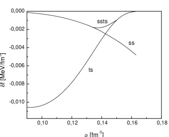
Figure 4: Free energy density, measured from that of the normal state, for SS, TS and SS–TS superfluid states at zero temperature.

One can see that in the density interval $\varrho_{1}<\varrho<\varrho_{m}$ the TS superfluid phase is thermodynamically most preferable as compared with other phases, and at $\varrho_{m}<\varrho<\varrho_{2}$ the SS superfluid state wins competition for thermodynamic stability. In both cases the mixed SS–TS state appears as a result of a phase transition in density from a thermodynamically less favorable one–gap superfluid state (SS state, if $\varrho_{1}<\varrho<\varrho_{m}$, and TS state, if $\varrho_{m}<\varrho<\varrho_{2}$) and corresponds to a metastable state in superfluid nuclear matter. In Fig. 5 we show the difference between the free energy densities of superfluid and normal states as a function of temperature. Fig. 5(a) corresponds to the branching of the SS–TS mixed state from the one–gap SS solution at fixed density in the range $\varrho_{1}<\varrho<\varrho_{m}$, and Fig. 5(b) depicts branching from the one–gap TS solution at a density in the interval $\varrho_{m}<\varrho<\varrho_{2}$.

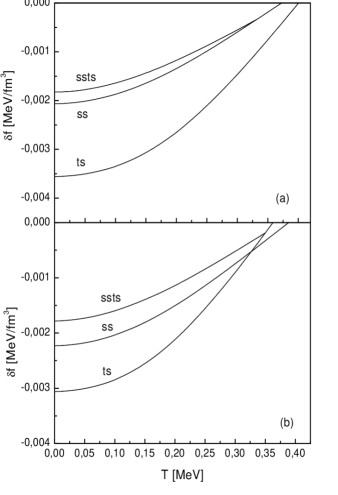
Figure 5: Difference between free energy densities of superfluid and normal states vs. temperature at density (a) $\varrho=0.138\ \mbox{fm}^{-3}$ and (b) $\varrho=0.140\ \mbox{fm}^{-3}$.

As seen, for all temperatures $T<T_{c}$, the SS–TS superfluid phase corresponds to a metastable state in superfluid nuclear matter.

CONCLUSION

We have considered the possibility of the formation of an anisotropic multi–gap condensate in superfluid symmetric nuclear matter, corresponding to the superposition of states with SS and TS pairing of nucleons. In the SS channel, pairing occurs with nonzero orbital angular momentum and hence the energy gap is an anisotropic function of momentum. The self-consistent equations for such two–gap states differ essentially from the equations of BCS theory and contain one-gap solutions (SS and TS) as particular cases. The analysis of the self-consistent equations at zero temperature in the logarithmic approximation shows that anisotropic multi–gap superfluid states can exist only under quite specific restrictions on the coupling constants $g_{0}$ and $g_{1}$, describing interaction of nucleons in the SS and TS pairing channels. Since the constants of the effective interaction depend on density, there are density domains, where one-gap or anisotropic two-gap solutions exist. Calculations with the effective SkP interaction, chosen as the model of the NN interaction, indicate that two-gap SS–TS states can arise in nuclear matter as a result of a phase transition in density from a one–gap SS or TS state. In the first case at critical density $g_{1}>g_{0}/3$, in the second, the opposite inequality is valid. Comparing free energies, branching occurs from thermodynamically less favorable one–gap solution and hence the anisotropic two–gap superfluid state corresponds to a metastable state in nuclear matter. Determination of the critical temperature $T_{c}$ of the transition to the SS–TS state as a function of density shows that the corresponding curve consists of two branches. One of them is related to the appearance of a SS–TS anisotropic state as a result of branching at $T_{c}$ from the one–gap SS solution, another is related to branching from the one–gap TS solution. Studying the temperature behavior of the order parameters shows that mixed two–gap solutions exist for temperatures $T<T_{c}$. Comparison of free energies leads to the conclusion that the anisotropic SS–TS phase represents a metastable state for the whole temperature interval $T<T_{c}$. Calculations show that mixed SS–TS states exist in a density domain, that is close to nuclear matter saturation density, in contrast to TS–ST mixed states, which only exist in the low density domain of nuclear matter.

Acknowledgement. A.I. is grateful for the hospitality and support of Rostock University, where a significant part of this work was completed. Discussions with S. Peletminsky and A. Yatsenko are gratefully appreciated. A.I. acknowledges the financial support of STCU (grant No. 1480).

References

- (1) A. Bohr and B.R. Mottelson, Nuclear structure (Benjamin, New York, 1969), Vol. 1.
- (2) P. Ring and P. Schuck, The Nuclear Many–Body Problem (Springer, New York, 1980).
- (3) A. Goodman, Nucl. Phys. A352, 30 (1981); A352, 45 (1981); A369, 365 (1981).
- (4) G. Röpke, A. Schnell, P. Schuck, and U. Lombardo, Phys. Rev. C 61, 024306 (2000).
- (5) Th. Alm, B.L. Friman, G. Röpke, and H. Schulz, Nucl. Phys. A551, 45 (1993).
- (6) M. Baldo, U. Lombardo, and P. Schuck, Phys. Rev. C 52, 975 (1995).
- (7) Th. Alm, G. Röpke, A. Sedrakian, and H. Schulz, Nucl. Phys. A604, 491 (1996).
- (8) A. Sedrakian, T. Alm, and U. Lombardo, Phys. Rev. C 55, R582 (1997).
- (9) A. Goodman, Phys. Rev. C 60, 014311 (1999).
- (10) W. Satula and R. Wyss, Phys. Rev. Lett. 86, 4488 (2001); 87, 052504 (2001).
- (11) A.I. Akhiezer, A.A. Isayev, S.V. Peletminsky, and A.A. Yatsenko, Phys. Lett. B 451, 430 (1999).
- (12) A.A. Isayev, Phys. Rev. C 65, 031302(R) (2002).
- (13) A.I. Akhiezer, V.V. Krasil’nikov, S.V. Peletminsky, and A.A. Yatsenko, Phys. Rep. 245, 1 (1994).
- (14) J. Dobaczewski, H. Flocard, and J. Treiner, Nucl. Phys. A422, 103 (1984).
- (15) P.-G. Reinhard, D.J. Dean, W. Nazarewicz, J. Dobaczewski, J.A. Maruhn, and M.R. Strayer, Phys. Rev. C 60, 014316 (1999).
- (16) R.K. Su, S.D. Yang, and T.T.S. Kuo, Phys. Rev. C 35, 1539 (1987).
- (17) M.F. Jiang and T.T.S. Kuo, Nucl. Phys. A481, 294 (1988).
- (18) A.I. Akhiezer, A.A. Isayev, S.V. Peletminsky, A.P. Rekalo, and A.A. Yatsenko, Zh. Eksp. Teor. Fiz. 112, 3 (1997) [Sov. Phys. JETP 85, 1 (1997)].
- (19) A.I. Akhiezer, A.A. Isayev, S.V. Peletminsky, and A.A. Yatsenko, Phys. Rev. C 63, 021304(R) (2001).