Quantum effects with an X-ray free electron laser

Abstract

A quantum kinetic equation coupled with Maxwell’s equation is used to estimate the laser power required at an XFEL facility to expose intrinsically quantum effects in the process of QED vacuum decay via spontaneous pair production. A $9\,$TW-peak XFEL laser with photon energy $8.3\,$keV could be sufficient to initiate particle accumulation and the consequent formation of a plasma of spontaneously produced pairs. The evolution of the particle number in the plasma will exhibit non-Markovian aspects of the strong-field pair production process and the plasma’s internal currents will generate an electric field whose interference with that of the laser leads to plasma oscillations.

X-ray free electron laser (XFEL) facilities are planned at SLAC slac : namely the Linac Coherent Light Source (LCLS), and as part of the $e^{-}\,e^{+}$ linear collider project (TESLA) at DESY desy . They propose to provide narrow bandwidth, high power, short-length laser X-ray pulses, with good spatial coherence and tunable energy. It is anticipated that the realisable values of these parameters will enable studies of completely new fields in X-ray science, with applications in atomic and molecular physics, plasma physics, and many other fields desy .

A unique ability of these facilities is to provide very high peak power densities. For example, a $P=0.2\,$TW-peak laser at a wavelength of $\lambda=0.4\,$nm, values which are reckoned achievable with current technology desy , can conceivably produce a peak electric field strength

$$E_{a}=\sqrt{\mu_{0}c\,P/(\pi\lambda^{2})}\approx 1.2\times 10^{16}\,{\rm V/m}\,.$$ (1)

Boosting $P$ to $1\,$TW and reducing $\lambda$ to $0.1\,$nm, which is theoretically possible Chen , would yield an order-of-magnitude increase: $E_{g}=1.1\times 10^{17}\,$V/m. Electric fields of this strength are sufficient for an experimental verification of the spontaneous decay of the QED vacuum Fried ; Ringwald ; popov ; bastiprl .

It is a long standing prediction that the QED vacuum is unstable in the presence of a strong, constant electric field, decaying via the production of $e^{-}\,e^{+}$ pairs Schwinger . In such fields, appreciable particle production is certain if the strength exceeds $E_{\rm cr}:=m_{e}^{2}/e=1.3\times 10^{18}\,{\rm V/m}$. (We subsequently use $\hbar=c=1$.) The proposed XFEL facilities could generate $E\approx 0.1\,E_{\rm cr}$. (NB. Here “constant” means that the field must be uniform over time- and length-scales much greater than the electron’s Compton wavelength: $1/m_{e}\approx 0.4\,$pm.)

A single laser beam cannot produce pairs Troup . (For a light-like field $F_{\mu\nu}F^{\mu\nu}=0$ and hence the vacuum survival probability is equal to one.) Nevertheless, if two or more coherent beams are crossed and form a standing wave at their intersection, one can hypothetically produce a region in which there is a strong electric field but no magnetic field. The radius of this spot volume is diffraction limited to be larger than the laser beams’ wavelength: $r_{\sigma}\gtrsim\lambda$, and the interior electric field could be approximately constant on length-scales approaching this magnitude. The period of the electric field is also determined by $\lambda$. Hence at an XFEL facility one might satisfy the length-scale uniformity conditions noted above.

However, the planned laser pulse duration: $\tau_{\rm coh}\sim 100\,$fs, is large compared to the laser period: $\tau_{\gamma}\sim 1\,$as, and thus the time-dependence of the electric field in the standing wave may materially affect the pattern of observed pair production; i.e., vacuum decay might be expressed via time-dependent pair production. This possibility can only be explored using methods of non-equilibrium quantum field theory BrezinPopov or an equivalent quantum kinetic theory basti ; kme ; sms . The latter procedure was employed in Ref. bastiprl , wherein it was shown that pair production occurs in cycles that proceed in tune with the laser frequency. While that does not lead to significant particle accumulation, the peak density of produced pairs is frequency independent, with the consequence that several hundred pairs could be produced per laser period.

The proposed XFEL facilities offer a first real chance of observing the decay of QED’s vacuum, a profound and nonperturbative quantum field theoretical effect. Nevertheless, with a quantum Vlasov equation, one can ask for more. This equation yields the time-dependence of the single particle distribution function: $f(\vec{p},t):=\langle a^{\dagger}_{\vec{p}}(t)\,a_{\vec{p}}(t)\rangle$, and hence can be used to estimate the laser power required to achieve an accumulation of $e^{-}\,e^{+}$ pairs via vacuum decay. Furthermore, in quantum field theory the particle production process is necessarily non-local in time; i.e., non-Markovian, and dependent on the particles’ statistics. These features are preserved by the source term in the Vlasov equation. (The Schwinger source term is recovered in a carefully controlled weak-field limit kme .) Consequently, one can identify the laser parameters necessary to expose negative energy elements in the particle wave packets. The system exhibits this core quantum field theoretical feature when the time between production events is commensurate with the electron’s Compton wavelength. Along with accumulation comes the possibility of plasma oscillations, generated by feedback between the laser-produced electric field and the field associated with the production and motion of the $e^{-}\,e^{+}$ pairs; and also collisions. (These features are reviewed in Ref. bastirev .)

We model an “ideal experiment,” and assume $r_{\sigma}=\lambda$ and a nonzero electric field constant throughout this volume while the magnetic field vanishes identically. This is impossible to achieve in practice and therefore the field strengths actually achievable will be weaker than we suppose. Hence our estimates of the laser parameters will be lower bounds. Our model is represented by

$${\vec{E}}_{\rm ext}(t)=(0,0,E_{0}\,\sin\Omega t\,)\,,\;\Omega=2\pi/\lambda\,.$$ (2)

Particle production occurs throughout the coherence spike length, $\tau_{\rm coh}$. However, collisions and radiation may become important as time progresses and therefore, to simplify our analysis, we focus on the first $100$ laser periods; i.e., the first $\sim 0.1$% of the laser pulse.

In spatially homogeneous fields the kinetic equation has the form

$$\frac{d\,f({\vec{p}},t)}{dt}=S({\vec{p}},t)+C({\vec{p}},t)\,,$$ (3)

where $S({\vec{p}},t)$ is a source term describing particle production and $C({\vec{p}},t)$ is a collision term, which properly includes annihilation. The form is intuitive: the rate of change in the single particle distribution function, $f(\vec{p},t)$, is determined by competition between particle production, and collisions and annihilation. The source term can be calculated directly using quantum mean field theory basti ; kme . The collision term, however, is more complicated and not directly accessible in the mean field approximation. It only becomes important, though, in dense plasmas and because we deliberately avoid that situation, we proceed by setting $C\equiv 0$.

The distribution of particles is described by $f(\vec{p},t)$. These particles are accelerated by $E_{\rm ext}(t)$, and the associated currents generate an opposing electric field, $E_{\rm int}(t)$. It is the sum: $E(t)=E_{\rm ext}(t)+E_{\rm int}(t)$, which is finally responsible for particle production. Thus, to properly represent the system’s evolution, one must solve a Vlasov equation coupled with Maxwell’s equation epjc :

$$\frac{df(\vec{p},t)}{dt} = \frac{eE(t)\varepsilon_{\perp}^{2}}{2\omega^{2}({\vec{p}},t)}\int_{0}^{t}dt^{\prime}\frac{eE(t^{\prime})\big{[}1-2f({\vec{p}},t^{\prime})\big{]}}{\omega^{2}({\vec{p}},t^{\prime})}$$ (4)

$$\qquad\qquad\times\cos\left[2\int_{t^{\prime}}^{t}d\tau~{}\omega({\vec{p}},\tau)\right],$$

$${\dot{E}}_{int}(t) = -4e\int\!\frac{d^{3}p}{(2\pi)^{3}}\,\frac{1}{\omega({\vec{p}},t)}\Biggl{[}p_{\|}f({\vec{p}},t)$$ (5)

$$+\frac{\omega^{2}({\vec{p}},t)}{eE(t)}\frac{d\,f({\vec{p}},t)}{d\,t}-\,\frac{e\dot{E}(t)\,\varepsilon_{\perp}^{2}}{8\,\omega^{4}({\vec{p}},t)}\Biggr{]},$$

with: ${\vec{p}}=({\vec{p}}_{\perp},p_{3})$; $\varepsilon_{\perp}^{2}=m_{e}^{2}+p_{\perp}^{2}$; $\omega^{2}({\vec{p}},t)=\varepsilon_{\perp}^{2}+p_{\|}^{2}(t)$, $p_{\|}(t)=p_{3}-e\,A(t)$.

Quantum statistics affect the production rate through the term “$[1-2\,f]$” in Eq. (4), which ensures that no momentum state has more than one spin-up and one spin-down fermion. In addition, both this factor and the “$\cos$” term introduce non-Markovian character to the system: the first couples in the history of the distribution function’s time evolution; the second, that of the field.

There are two control parameters in Eq. (4): the laser field strength, $E_{0}$, and the wavelength, $\lambda$. We fix $\lambda=0.15\,$nm, which is achievable at the proposed XFELs. (NB. By assumption, the volume in which particles are produced increases with $\lambda^{3}$ whereas the field strength decreases with $1/\lambda$: there is merit in optimising $\lambda$.) Our study will expose additional phenomena that become observable with increasing $E_{0}$.

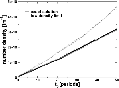
Figure 1: Number density calculated with $E_{0}=0.5\,E_{cr}$. Solid line: solution of Eqs. (4), (5); dotted line: solution obtained using a low density approximation to $S({\vec{p}},t)$, Eq. (11). The oscillations are tied to the laser frequency, see Eq. (7).

The particle number density:

$$n(t)=2\int\frac{d^{3}p}{(2\pi)^{3}}\,f(\vec{p},t)\,,$$ (6)

is plotted in Fig. 1 for $E=0.5\,E_{cr}$. Our results for $T=t/\lambda\lesssim 100$ are accurately fitted by

$$n(T;E_{0}) = a_{0}(E_{0})\,\sin^{2}2\pi T\,+\rho(T,E_{0})\,T\,,$$ (7)

$$\rho(T,E_{0}) = \rho(E_{0})+\rho^{\prime}(E_{0})\,T\,.$$ (8)

We can therefore use $\rho(T,E_{0})$ to quantify the rate of particle accumulation. This rate is very small for $E_{0}\lesssim 0.2\,E_{\rm cr}$ bastiprl and, while noise in $n(t)$ prevents a reliable numerical determination of $\rho$, $\rho^{\prime}$, it is nevertheless clear that in this case lengthening $\tau_{\rm coh}$ will not materially increase the number of particles produced.

It is apparent from Fig. 1, however, that the situation is very different for $E_{0}=0.5\,E_{\rm cr}$. The solid curve is described by Eq. (7), with $a_{0}=1.2\times 10^{-11}\,$fm^-3, $\rho=5.4\times 10^{-12}\,$fm${}^{-3}\,$period${}^{-1}\!$, $\rho^{\prime}/\rho=0.0033/$period. Clearly, the accumulation rate is approximately constant.

Solving the coupled system of Eqs. (4), (5) numerically is straightforward but time consuming. We have repeated the procedure for a range of values of $E_{0}$ and plotted the calculated values of $\rho(E_{0})$ in Fig. 2. These results can be used to obtain a rough estimate of the accumulated number density via: $n(T,E_{0})\approx\rho(E_{0})\,T$. We also plot:

$$\rho_{\rm S}=a_{S}\,\frac{m_{e}^{4}\lambda}{4\pi^{3}}\left[\frac{E_{0}}{E_{\rm cr}}\right]^{2}\,{\rm e}^{-b_{S}\,\pi E_{\rm cr}/E_{0}},\;a_{S}=1,\,b_{S}=1\,;$$ (9)

i.e., the Schwinger rate. As can be anticipated from the energy budget, the constant-field Schwinger rate bounds our results from above. This comparison provides a context for the estimates in Ref. Ringwald .

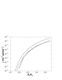
Figure 2: Solid line: accumulation rate, $\rho(0,E_{0})$, Eq. (8); dashed line: Schwinger rate, Eq. (9); dot-dashed line: Eq. (9) with $a_{S}\to a=0.305$, $b_{S}\to b=1.06$.

In Fig. 3 we plot the peak particle number density, $n(t_{k}^{>})$, where $t_{k}^{>}=(4k-3)\lambda/4$ is the time at which $E(t)$ is maximal during laser period no. $k$. The figure displays a qualitative change in the rate of particle production with increasing laser field strength. [$n(k\lambda)\approx n(t_{k}^{>})$ if and only if there is significant particle accumulation, otherwise $n(k\lambda)\ll n(t_{k}^{>})$.]

That change is emphasised by Table 1, which reports

$$N(t_{k}^{>},E_{0}):=\sigma\,n(t_{k}^{>},E_{0})\,;$$ (10)

i.e., the peak particle number.

Table 1: Peak particle number, Eq. (10), at selected values of the laser field strength, $E_{0}$ in Eq. (2), with $k=50$.

$\displaystyle E_{0}/E_{cr}$	0.1	0.2	0.3	0.4	0.5
$\displaystyle N_{\sigma}\,(\times 10^{3})$	1.3	5.4	17.9	148	1110

For $E_{0}\lesssim 0.25\,E_{\rm cr}$ there is no significant accumulation of particles: $N(t_{0}^{>},E_{0})\approx N(t_{10}^{>},E_{0})$, etc., just as observed in Ref. bastiprl . However, for $E_{0}>0.25\,E_{\rm cr}$ there are more particle pairs after each successive laser period; e.g., $E_{0}=0.35\,E_{\rm cr}$ brings an order of magnitude increase in $N$ over the first $100$ laser periods. At such values of $E_{0}$ one is in a domain where numerous electrons and positrons produced in a single period are accelerated to relative longitudinal momenta that are sufficient to materially inhibit annihilation. This ensures that many pairs remain when the next burst of production occurs. Consequently $N(t_{k}^{>},E_{0})$ grows considerably with increasing $k$. (NB. Accumulation means collisions can become important and should be included in the kinetic equation if quantitatively reliable results are required. As we neglect these effects we do not follow the system’s evolution into the high density regime.)

In the low density limit: $f(\vec{p},t)\ll 1$, the distribution function disappears from the right hand side of Eq. (4), which then yields an algebraic solution:

$$f^{\rm ld}({\vec{p}},t) = \int_{0}^{t}d\tau\frac{eE(\tau)\varepsilon_{\perp}^{2}}{2\omega^{2}({\vec{p}},t)}\int_{0}^{\tau}dt^{\prime}\frac{eE(t^{\prime})}{\omega^{2}({\vec{p}},t^{\prime})}$$ (11)

$$\qquad\times\cos\left[2\int_{t^{\prime}}^{t}d\tau^{\prime}~{}\omega({\vec{p}},\tau^{\prime})\right].$$

We anticipated this in Fig. 1, which contrasts the low-density result with the complete solution for $E_{0}=0.5\,E_{\rm cr}$, which we now know generates significant particle accumulation. The comparison emphasises that, with particle accumulation, quantum statistical effects in the source term are observable. These effects are essentially non-Markovian. The difference grows with increasing field strength because Pauli blocking becomes more important with increasing fermion density.

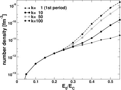
Figure 3: Peak particle number density versus laser field strength. There is a striking qualitative change at $E_{0}\approx 0.25\,E_{\rm cr}$, which marks the onset of particle accumulation.

We now return to Eq. (5); i.e., Maxwell’s equation: $\dot{E}=-j$. The right hand side has two components: the first term, proportional to $f(\vec{p},t)$, is a conduction current tied to the particles’ motion; and the last two terms express a polarisation current that is tied to the pair production rate bloch . While these terms remain small the total electric field is determined solely by the applied laser beams. However, in the domain of particle accumulation the internal currents can modify the electric field in the system, so that the coupling between Eqs. (4) and (5) becomes important. This marks the onset of field-current feedback, which can lead to plasma oscillations.

Figure 4 depicts the ratio of the internal and external currents. Evidently, with the field strengths realisable at proposed XFELs, the internal current is negligible. However, with the onset of particle accumulation the ratio grows with the number of elapsed laser periods and, since there are roughly $10^{5}$ periods in a given pulse, feedback will necessarily come to affect the plasma’s behaviour at some stage in its evolution. Notably, for $E_{0}=0.5\,E_{\rm cr}$ that happens very early; i.e., after only $0.1\,$% of the lifetime of the pulse, and feedback will have observable consequences. (NB. Our full calculations incorporate this effect but the result is a signal that less complete estimates will become more unreliable in the domain of particle accumulation.) A proper analysis of the observable effects of feedback must also include an accurate description of collisions, which can act to damp plasma oscillations epjc .

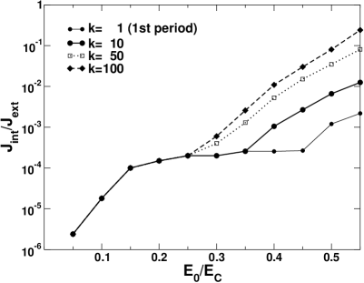
Figure 4: Ratio of the peak internal and external currents, plotted as function of $E_{0}/E_{cr}$. Field-current feedback becomes important for $E_{0}\gtrsim 0.25\,E_{cr}$.

We have explored the possibility of $e^{-}\,e^{+}$ pair production using XFEL beams as a parameter-free application of nonequilibrium quantum mean-field theory. An idealised model of the laser electric field was used as input to a quantum Vlasov equation coupled with Maxwell’s equation. Decay of the QED vacuum is likely to be observed at proposed XFEL facilities. However, we showed that additional phenomena become observable if the peak power is increased by a factor of $\sim 9$. Then the particles produced from the QED vacuum accumulate to form a plasma, which is not achieved at the DESY and SLAC facilities. That plasma’s behaviour will expose essential quantum field theoretical aspects of the pair production process, which are absent from the Schwinger formula. While this power is insufficient to expose negative energy components in the electron wave packets, it can reveal the non-Markovian nature of pair production; i.e., the feature that the appearance of a new pair is not independent of the production of the preceding pairs nor the evolution of the plasma before this new pair is produced. With this peak power the accumulated charged pairs are also likely to generate internal currents that interfere with the applied laser field so that the plasma exhibits charge-density fluctuations; i.e., plasma oscillations. An accurate prediction of this effect’s observable consequences requires a realistic collision term in addition to the proper source.

We thank R. Alkofer and A. Ringwald for discussions. This work was supported by the Deutsche Forschungsgemeinschaft, under contract nos. Ro 1146/3-1 and SCHM 1342/3-1; the US Department of Energy, Nuclear Physics Division, under contract no. W-31-109-ENG-38; the US National Science Foundation under grant no. INT-0129236; and benefited from the resources of the US National Energy Research Scientific Computing Center.

References

- (1) J. Arthur, et al. [LCLS Design Study Group Collaboration], “Linac coherent light source (LCLS) design study report,” SLAC-R-0521 (1998).
- (2) TESLA Technical Design Report, Part V: The X-Ray Free Electron Laser, edited by G. Materlik and Th. Tschentscher, available at http://tesla.desy.de/new_pages/TDR_CD/start.html
- (3) P. Chen and C. Pellegrini, in Proceedings of the 15th Advanced ICFA Beam Dynamics Workshop on Quantum Aspects of Beam Physics, Monterey, CA, 1998, edited by P. Chen (World Scientific, Singapore, 1999) pp. 571-576.
- (4) H.M. Fried, Y. Gabellini, B.H.J. McKellar and J. Avan, Phys. Rev. D 63, 125001 (2001).
- (5) A. Ringwald, Phys. Lett. B 510, 107 (2001); A. Ringwald, hep-ph/0112254.
- (6) V.S. Popov, JETP Lett. 74, 133 (2001) [Pisma Zh. Eksp. Teor. Fiz. 74, 151 (2001)].
- (7) R. Alkofer, et al., Phys. Rev. Lett. 87, 193902 (2001).
- (8) J. Schwinger, Phys. Rev. 82, 664 (1951).
- (9) G.J. Troup and H.S. Perlman, Phys. Rev. D 6, 2299 (1972).
- (10) E. Brezin and C. Itzykson, Phys. Rev. D 2, 1191 (1970); V.S. Popov and M.S. Marinov, Yad. Fiz. 16, 809 (1972) [Sov. J. Nucl. Phys. 16, 449 (1973)]; N.B. Narozhnyi and A.I. Nikishov, Zh. Eksp. Teor. Fiz. 65, 862 (1973) [Sov. Phys. JETP 38, 427 (1974)].
- (11) S.M. Schmidt, et al., Int. J. Mod. Phys. E 7, 709 (1998); S.A. Smolyansky, et al., hep-ph/9712377; S.M. Schmidt, A.V. Prozorkevich and S.A. Smolyansky, hep-ph/9809233.
- (12) Y. Kluger, E. Mottola, and J.M. Eisenberg, Phys. Rev. D 58, 125015 (1998).
- (13) J.C.R. Bloch, C.D. Roberts and S.M. Schmidt, Phys. Rev. D 61, 117502 (2000); D.V. Vinnik, et al., nucl-th/0202034.
- (14) C.D. Roberts and S.M. Schmidt, Prog. Part. Nucl. Phys. 45, S1 (2000).
- (15) D.V. Vinnik, et al., Eur. Phys. J. C 22, 341 (2001).
- (16) J.C.R. Bloch, et al., Phys. Rev. D 60, 116011 (1999).