Path-integral hadronization for the nucleon and its interactions

Abstract

Nucleon structure and the origin and nature of the nuclear force are investigated in the context of a QCD-based effective field theory and the path-integral method of hadronization. We start from a microscopic model of quarks and diquarks where the gluons have been integrated out. In particular, we use the chiral Nambu-Jona-Lasinio model to describe quark dynamics and assume that the nucleon can be conceived as a quark-diquark relativistic bound state. The hadronization method is then used to rewrite the problem in terms of the physical meson and nucleon degrees of freedom. Next, by employing a loop and derivative expansion of the resulting quark/diquark determinants, we arrive at an effective chiral meson-nucleon Lagrangian. Nucleon properties such as mass, coupling constants, electromagnetic radii, anomalous magnetic moments, and form factors are derived using a theory of at most two free parameters.

I Introduction

The central problem in nuclear physics remains to understand the origin and nature of the nuclear force. In spite of the belief that we have attained the fundamental theory for the strong interactions– Quantum chromodynamics (QCD), this theory still eludes a satisfactory and complete description. The basic problem of QCD is that its natural and fundamental degrees of freedom, quarks and gluons, are not the observable baryon and meson states of the strong interaction. Thus bridging the missing link between the fundamental and observable degrees of freedom stands as one of the stark challenges of nuclear/elementary particle physics today. Although we do have an ab initio approach to solve this problem, that is lattice QCD, this endeavor is still miles away from achieving such a goal. This naturally motivates us to resort to non-perturbative QCD-based approaches of which this study is one.

In the present paper, we address this lingering missing link by deriving a chiral meson-nucleon Lagrangian from a microscopic model of quarks and diquarks using path-integral methods. Chiral symmetry and its spontaneous breaking have consistently proven to be key concepts in understanding meson and baryon structure and many features of the nuclear force Weinberg (1967); S. Coleman and Zumino (1969); C. Callan and Zumino (1969); Ebert and Volkov (1981). The gist of this paper is as following: We start from a QCD-based effective field theory to describe quark dynamics where the gluons have been integrated out. This is the SU(2)${}_{L}\;\times$ SU(2)_R Nambu-Jona-Lasinio (NJL) model that accommodates most of QCD symmetries Nambu and Jona-Lasinio (1961); Ebert and Reinhardt (1986). Guided by general principles, we then assume that the nucleon can be described as quark-diquark correlations and introduce diquarks Ida and Kobayashi (1966); Lichtenberg et al. (1968) as elementary fields in the problem. This assumption hinges upon the dynamical fact that two quarks can combine to form a color anti-triplet leading with the third quark to the formation of a color-singlet bound state, a baryon. Moreover, this assertion is vindicated by a mounting experimental evidence that diquarks play a dynamical role in hadrons Vogl and Weise (1991); Anselmino et al. (1993); Anselmino and Predazzi (1989); Donnachie and Landshoff (1980); Close and Roberts (1981); Fredriksson et al. (1982); Kroll et al. (1991); Stech (1987); Neubert and Stech (1991).

We verify that only two kinds of diquarks are relevant for nucleons: the scalar isoscalar and the axial-vector isovector. By introducing composite meson and nucleon fields through the method of path-integral hadronization and then using a loop and derivative expansion of the resulting quark/diquark determinants, we arrive at an effective chiral meson-nucleon Lagrangian. The path-integral hadronization used here consists of two steps: bosonization to produce mesons as quark-antiquark correlations and what we label as “fermionization” which generates baryons as quark-diquark correlations. In our model, mass, coupling constants, electromagnetic radii, anomalous magnetic moments, and form factors of the composite nucleon are calculated in terms of at most two free parameters.

In this fashion, our treatment parallels, in the sense of calculating nucleon physical observables, the approach of using the Faddeev equation Faddeev (1961a, b) for three quark states Alkofer et al. (1992); Ishii et al. (1993a, b); Meyer (1994), or the approach of using static quark exchange Hellstern and Weiss (1995), the Salpeter equation Salpeter (1952); Keiner (1996a, b) or the fully relativistic Bethe-Salpeter equation Salpeter and Bethe (1951); Hellstern et al. (1997); Oettel et al. (1998) for a quark-diquark system. Nonetheless, our formalism yields, in addition to nucleon observables, a Lagrangian of the quantum hadrodynamics (QHD) type Walecka (1974); Serot and Walecka (1986) that describes the rich meson-nucleon interactions in a fully covariant and chirally symmetric formalism.

While this program is applied to the case of deriving an effective Lagrangian for nucleons and mesons, it is certainly of general nature and can possibly be applied alternatively to yield prolifically other baryons and their interactions such as the $\Delta$ particle. Moreover, the idea of using path-integral techniques to transform a Lagrangian from its fundamental to its composite degrees of freedom is a powerful concept in physics of immense impact and utility. As a matter of fact, the authors of Ref. Ichinose et al. (2001) have recently invoked such path-integral techniques in their study of high-temperature superconductivity. They succeeded in doing so by converting a model of strongly-correlated electrons into an effective U(1) gauge field theory in terms of composite fields.

The use of path-integral hadronization to derive a meson-baryon Lagrangian has been introduced in Ref. Cahill (1989); Reinhardt (1990); Ebert and Kaschluhn (1992) and applied to baryons with heavy quarks Ebert et al. (1996, 1998). Based on these ideas, the authors of Ref. Ebert and Jurke (1998) attempted to construct such an effective Lagrangian for the nucleon using only scalar diquarks. They derived correctly the structure of the meson-nucleon Lagrangian, proved the Goldberger-Treiman relation and attempted to evaluate the axial-vector coupling constant $g_{A}$ as an application of their formalism. Their analysis and numerics for $g_{A}$ contain, however, few problems as well as an uncertainty due to the lack of a proper gauge-invariant regularization scheme. In the present paper, we extend their work by deriving the structure of the corresponding Lagrangian using both axial-vector and scalar diquarks, employ a gauge-invariant regularization scheme throughout our analysis, and verify the Ward-Takahashi identity and the Goldberger-Treiman relation. Furthermore, we present a full numerical study of various nucleon observables for the case of scalar diquarks drawing special attention to the role of an intrinsic diquark form factor. We concentrate our analysis first on the scalar-diquark case for simplicity and due to the predicted dominance of this type of diquark in the nucleon Cahill et al. (1987); Reinhardt (1990); Vogl (1990); Mineo et al. (2002). Thus after more than ten years since the introduction of the idea of path-integral hadronization, this formalism is finally used to speak itself in calculating nucleon structure and its observables.

The paper has been organized as follows. In Sec. II a microscopic model for quarks, diquarks, and their interactions is developed and meson and nucleon fields are introduced as auxiliary fields in the problem. The hadronization method is then invoked in Sec. III to rewrite the microscopic Lagrangian in terms of composite meson and nucleon fields. Next, a loop and derivative expansion is employed to calculate several terms in the Lagrangian including the nucleon self-energy and electromagnetic vertex. The issue of regularization is also examined and the Ward-Takahashi identity and the Goldberger-Treiman relation are verified. In Sec. IV a full numerical study for the nucleon is presented. Finally a summary and conclusions are provided in Sec. V as well as a discussion of some of the challenges and opportunities that remain.

II A microscopic model of quarks, diquarks and their interactions

II.1 Nambu-Jona-Lasinio Model

In our model we treat the quarks using the NJL model which is a successful effective field theory where quarks interact through a four-point local fermion-fermion coupling. The highlights of the model are its incorporation of all global symmetries of QCD as well as its prediction of many features of QCD such as dynamical chiral symmetry breaking and its restoration  Ebert and Reinhardt (1986); Vogl and Weise (1991); Hatsuda and Kunihiro (1994); Ebert et al. (1994). Moreover, this model has been motivated, if also not derived, using lattice QCD Kawamoto and Smit (1981), continuum QCD  Hatsuda and Kunihiro (1994); Ebert et al. (1994); Andrianov et al. (1987); Ball (1990); Reinhardt (1991); Bijnens et al. (1993), and Yang-Mills theories Schaden et al. (1990). The locality assumption of the model has been justified for low energy QCD  Schaden et al. (1990), and inspired by strong-coupling lattice quantum electrodynamics (QED) Gockeler et al. (1990); Vogl and Weise (1991). The main problem of the NJL model continues to be the absence of confinement. Therefore, the success of the model rests on observables that are insensitive to the details of confinement. It is noteworthy here that there exists various attempts to include the effects of confinement within the NJL model Belkov et al. (1993); Hatsuda and Kunihiro (1994).

We start from an NJL Lagrangian satisfying SU(2)${}_{L}\;\times$ SU(2)_R chiral symmetry:

$${\cal L_{\text{NJL}}}={\bar{q}}(i\hbox to0.0pt{/\hss}\partial-m_{0})q+\frac{G}{2}\left[({\bar{q}}q)^{2}+({\bar{q}}i\gamma_{5}\vec{\tau}q)^{2}\right]\;.$$ (1)

Here $q$ is the current quark field, $\vec{\tau}$ are the isospin (flavor) Pauli matrices, $G$ is the NJL coupling constant, and $m_{0}$ is the current quark mass which explicitly breaks chiral symmetry. The color and flavor indices are suppressed in this expression and assumed to be so for the rest of the paper unless explicitly shown. Starting from this Lagrangian, we construct the corresponding vacuum partition function as

$${\cal Z}={\mathcal{N}_{1}}\int{\mathcal{D}}q{\mathcal{D}}\bar{q}\;{\exp}\;i\int{\rm d}^{4}x\;\left[{\cal L_{\text{NJL}}}\right]\;,$$ (2)

where ${\mathcal{N}_{1}}$ is a normalization constant.

II.2 Introduction of meson fields

Composite scalar ($\sigma\sim\bar{q}q$) and pseudoscalar ($\vec{\pi}\sim\bar{q}i\gamma_{5}\vec{\tau}q$) meson fields are introduced as auxiliary fields in the problem. This is done by multiplying the NJL partition function of Eq. (2) by the term (with ${\mathcal{N}_{2}}$ being another normalization constant)

$${\mathcal{N}_{2}}\int{\mathcal{D}}\sigma{\mathcal{D}}\vec{\pi}\;{\exp}\;i\int{\rm d}^{4}x\;\left[-\frac{1}{2G}(\sigma^{2}+\vec{\pi}^{2})\right]\;.$$ (3)

At this stage, no modifications have been made to the underlying dynamics of the Lagrangian as this multiplicative factor is merely an overall constant in the partition function. We impose the following transformation:

$$\sigma \longrightarrow \sigma+G\bar{q}q\;,$$

$$\pi^{i} \longrightarrow \pi^{i}+G\bar{q}i\gamma^{5}\tau^{i}q\;,$$ (4)

in order to eliminate the quadratic terms ($\sim(\bar{q}q)^{2}$) of the NJL Lagrangian. Using translational invariance of the integration measure ${\mathcal{D}}\sigma{\mathcal{D}}\vec{\pi}$, this results in the expression:

$${\mathcal{N}_{3}}\int{\mathcal{D}}\sigma{\mathcal{D}}\vec{\pi}{\mathcal{D}}q{\mathcal{D}}\bar{q}\;{\exp}\;{i\int{\rm d}^{4}x\;\left[\bar{q}\left(i\hbox to0.0pt{/\hss}\partial-m_{0}-\sigma-i\gamma_{5}\vec{\tau}\cdot\vec{\pi}\right)q-\frac{1}{2G}(\sigma^{2}+\vec{\pi}^{2})\right]}\;.$$ (5)

The prescribed change in field variables is nothing but the Hubbard-Stratonovich transformation Stratonovich (1958); Hubbard (1959). We label the resulting Lagrangian as the “semi-bosonized” one since we have already introduced the boson (meson) fields but have not yet integrated over the quark ones. The current quark mass $m_{0}$ is then absorbed into the definition of the field $\sigma$ and the meson fields are further transformed according to the non-linear parameterization $\left[\sigma,\pi\right]\rightarrow\left[\sigma^{\prime},\Phi\right]$

$$\sigma+i\gamma_{5}\vec{\tau}\cdot\vec{\pi} = \left(m_{q}+\sigma^{\prime}\right){\exp}{\left(-\frac{i}{F_{\pi}}\gamma_{5}\vec{\tau}\cdot\vec{\Phi}\right)}\;,$$ (6)

where $F_{\pi}=93$ MeV is the pion decay constant and $m_{q}\equiv\langle\sigma\rangle_{0}$ is the constituent quark mass which is fixed through a gap equation in the meson sector  Ebert and Reinhardt (1986); Hatsuda and Kunihiro (1994); Ebert et al. (1994). Accordingly, the NJL Lagrangian is converted to

$${\cal L_{\text{NJL}}}=\delta{\cal L}_{\rm sb}\;-\;\frac{1}{2G}\left(\sigma^{\prime}+m_{q}\right)^{2}\;+\;{\bar{q}}\left[i\hbox to0.0pt{/\hss}\partial-\left(m_{q}+\sigma^{\prime}\right){\exp}\left({-\frac{\rm i}{F_{\pi}}\gamma_{5}\vec{\tau}\cdot\vec{\Phi}}\right)\right]q\;.$$ (7)

Here, the $\delta{\cal L}_{\rm sb}=\mathcal{O}(m_{0})$ is the symmetry-breaking mass term given by

$$\delta{\cal L}_{\rm sb}=\frac{m_{q}+\sigma^{\prime}}{16\kern 1.42262ptG}m_{0}\kern 2.84526pt{\rm tr}\left[{\exp}\left({-\frac{i}{F_{\pi}}\gamma_{5}{\vec{\tau}\cdot\vec{\Phi}}}\right)+{\rm h.c.}\right]\;,$$ (8)

where the trace is taken over flavor and Dirac indices.

II.3 Diquarks

In studying the Lorentz and flavor structure of the $qq$ correlations, we find five possible types: the scalar $\tilde{q}q$, pseudo-scalar $\tilde{q}i\gamma_{5}q$, vector $\tilde{q}\gamma_{\mu}q$, axial-vector $\tilde{q}\gamma_{\mu}\gamma_{5}q$, and tensor $\tilde{q}\sigma_{\mu\nu}q$ diquarks. Here $\tilde{q}\equiv q^{\rm T}C^{-1}\gamma_{5}i\tau_{2}$ where T stands for transpose and $C^{-1}=i\gamma_{2}\gamma_{0}$ is the inverse charge-conjugation matrix. Moreover, we identify two isospin structures for each of these five Lorentz $qq$ formations. Explicitly, we have an isoscalar and isovector diquarks by inserting $\openone$ and $\vec{\tau}$ between $\tilde{q}$ and ${q}$. It has to be noted here that the $\tilde{q}$ spinor has the same transformation properties as $\bar{q}$ in the Lorentz and isospin groups.

A question arises concerning how many of these ten diquarks are needed to form the nucleon. Using permutation symmetry and Fierz transformation, we have verified an earlier assertion Espriu et al. (1983) that only two diquark formations are independent for the nucleon if the nucleon field is to be written as a local operator of three quarks. This result is consistent with the fact that in constituent quark models Greiner and Schaefer (1994), the nucleon wave function is constructed using only scalar and axial-vector diquarks. Hence, we introduce two diquarks as elementary complex fields: ${\vec{D}}^{\mu}$ as an axial-vector isovector field with electric charge = {4/3, 1/3, -2/3} and $D$ as a scalar isoscalar field with a charge = {1/3}.

II.4 Quark-diquark interaction terms

Quark-diquark interaction terms are introduced to form the nucleon as a relativistic bound state of quarks and diquarks. We consider such an interaction in a local form. This is essentially the static approximation of solving the three-body equations for baryons within the NJL model Ishii et al. (1993b); Mineo et al. (2002). It is more convenient here, in terms of forming a chirally invariant quark-diquark couplings, to work with the chirally rotated “constituent” quark field $\chi$ defined by 

$$\chi\equiv\exp\left({-\frac{i}{F_{\pi}}\gamma^{5}\frac{\vec{\tau}}{2}\cdot\vec{\Phi}}\right)q\;.$$ (9)

The range of possible symmetry preserving interaction terms is limited . This provides a highly welcomed dynamical constraint in our treatment. Discarding for a moment interaction terms describing a possible scalar-axial-vector mixing (see Eq. (13) below), we may choose the following term for the quark-scalar-diquark interaction:

$${\cal{L}}_{qD}\sim\tilde{G}\;\left(\bar{\chi}D^{\dagger}\right)\left(D\chi\right)\;,$$ (10)

while we may select

$${\cal{L}}_{q{\vec{D}}^{\mu}}\sim\tilde{G}\;(\bar{\chi}\gamma^{\mu}\gamma^{5}\>\vec{\tau}\cdot{\vec{D}}^{\dagger}_{\mu})\;({\vec{D}}_{\nu}\cdot\vec{\tau}\>\gamma^{\nu}\gamma^{5}\chi)\;,$$ (11)

for the quark-axial-vector-diquark coupling. Our choice for the full interaction term is dictated by the need to produce the nucleon as a linear combination of axial-vector and scalar diquarks according to

$$B\;\;\sim\tilde{G}\;\left(\sin{\theta}\;{\vec{D}}_{\mu}\cdot\vec{\tau}\;\gamma^{\mu}\gamma^{5}\;\chi\;+\;\cos{\theta}\;D\;\chi\right)\;.$$ (12)

In the above expressions $\tilde{G}$ is the quark-diquark coupling constant with mass dimension $[\tilde{G}]=m^{-1}$, while $\theta$ is a mixing angle for the two diquark contributions. These are, as we shall discuss below (see Sub-Sec. IV.1), the only free parameters in our model.

II.5 Microscopic Lagrangian

Electromagnetic interactions are introduced in our model through the canonical method of covariant derivatives in the quark and diquark Lagrangians. We proceed to form the microscopic Lagrangian by batching the diquark contributions, the quark-diquark interaction terms including mixing, and the semi-bosonized NJL Lagrangian of Eq. (7) after the field transformations of Eq. (9), to obtain the following Lagrangian as our input model:

$${\cal L} = \bar{\chi}\;S^{-1}\;\chi\;-\;\frac{1}{2G}(\sigma^{\prime}+m_{q})^{2}\;+\;\delta{\cal L}_{\rm sb}\;+\;D^{\dagger}\;\Delta^{-1}\;D\;+\;{\vec{D}^{{\dagger}\;\mu}}\;{\tilde{\Delta}}^{-1}_{\mu\nu}\;\vec{D}^{\nu}\;+\;$$ (13)

$$\tilde{G}\left(\sin{\theta}\;\bar{\chi}\gamma^{\mu}\gamma^{5}\>\vec{\tau}\cdot{\vec{D}}^{\dagger}_{\mu}\;+\;\cos{\theta}\;\bar{\chi}D^{\dagger}\right)\;\left(\sin{\theta}\;{\vec{D}}_{\nu}\cdot\vec{\tau}\>\gamma^{\nu}\gamma^{5}\chi\;+\;\cos{\theta}\;D\chi\right)\;,$$

where

$$S^{-1} = S_{0}^{-1}\;+\;{\cal M}\;,$$ (14a)

$${\cal M} = -\left[\gamma^{\mu}\frac{\vec{\tau}}{2}\cdot\vec{\mathcal{V}}^{\pi}_{\mu}\;+\;\gamma^{\mu}\gamma^{5}\frac{\vec{\tau}}{2}\cdot\vec{\mathcal{A}}^{\pi}_{\mu}\;+\;\sigma^{\prime}\;+\;\gamma^{\mu}Q_{q}A^{\rm EM}_{\mu}\right]\;.$$ (14b)

Here $S^{-1}$ is the modified inverse propagator that includes the free inverse propagator $S_{0}^{-1}=(i\hbox to0.0pt{/\hss}\partial-m_{q})$ for the quark field and the interaction matrix ${\cal M}$. Note that $Q_{q}=\text{diag}\left(2/3,-1/3\right)$ is the quark charge. The ${\cal M}$ matrix contains all interaction vertices of the quark with meson and electromagnetic fields. The quark interacts with the pion through vector $\vec{\mathcal{V}}^{\pi}_{\mu}$ and axial-vector $\vec{\mathcal{A}}^{\pi}_{\mu}$ functions of the pion field. These arise from the derivative term $i\hbox to0.0pt{/\hss}\partial$ following the transformation of Eq. (9). Precisely, these functions are defined through the Cartan decomposition ($\vec{\xi}\equiv\frac{\vec{\Phi}}{F_{\pi}}$):

$${\exp}\left({-\frac{i}{2}\gamma^{5}{\vec{\tau}\cdot\vec{\xi}}}\right)\;\partial_{\mu}\ {\exp}\left({\frac{i}{2}\gamma^{5}{\vec{\tau}\cdot\vec{\xi}}}\right)\;=\;{\textstyle\frac{i}{2}\;\gamma^{5}\;{\vec{\tau}}}\cdot\vec{\mathcal{A}}^{\pi}_{\mu}(\xi)\;+\;{\textstyle\frac{i}{2}\;{\vec{\tau}}}\cdot\vec{\mathcal{V}}^{\pi}_{\mu}(\xi)\;.$$ (15)

The ${\cal M}$ matrix also encompass pion-photon and weak gauge boson vertices which are not shown for brevity.

In the above Lagrangian, we use the modified scalar diquark inverse propagator

$$\Delta^{-1}=\Delta_{0}^{-1}+iQ_{S}A^{\rm EM}_{\mu}(\overrightarrow{\partial^{\mu}}-\overleftarrow{\partial^{\mu}})\;,$$ (16)

and the modified axial-vector diquark inverse propagator

$${\tilde{\Delta}}^{-1}_{\mu\nu}={{\tilde{\Delta}}_{0}\;}^{-1}_{\mu\nu}\;+\;iQ_{A}\left[(A^{\rm EM}_{\mu}\overleftarrow{\partial_{\nu}}-A^{\rm EM}_{\nu}\overrightarrow{\partial_{\mu}})\;-\;g_{\mu\nu}A^{\rm EM}_{\alpha}(\overleftarrow{\partial^{\alpha}}-\overrightarrow{\partial^{\alpha}})\right]\;,$$ (17)

where we have omitted ${\cal O}(Q_{S}^{2})$ and ${\cal O}(Q_{A}^{2})$ terms for brevity. Each of these expressions includes the free inverse propagator as the kinetic and mass term, and the electromagnetic interaction vertex. Explicitly, the free inverse propagator for the scalar diquark is

$$\Delta_{0}^{-1}=-(\partial^{2}+M_{S}^{2})\;,$$ (18)

while the one for the axial-vector diquark is

$${\tilde{\Delta}}^{-1}_{\mu\nu}=\openone\otimes[g_{\mu\nu}(\partial^{2}+M_{A}^{2})-\partial_{\mu}\partial_{\nu}]\;,$$ (19)

where $\openone$ is the unit matrix in the three-dimensional isospace. Here $Q_{S}=1/3$ and $Q_{A}=\text{diag}\left(4/3,1/3,-2/3\right)$ are the charges of the scalar and axial-vector diquarks respectively. The modified axial-vector diquark propagator encompasses (not shown) weak interaction terms.

II.6 Introduction of nucleon fields

There is still one missing component in our microscopic model: collective nucleon fields. Therefore, a nucleon field $B$ is introduced as an auxiliary one by multiplying the partition function of the Lagrangian of Eq. (13) by the term

$${\mathcal{N}_{4}}\int{\mathcal{D}}B{\mathcal{D}}\bar{B}\;{\exp}\;i\int{\rm d}^{4}x\;\left[-\frac{1}{\tilde{G}}\bar{B}B\right]\;,$$ (20)

where ${\mathcal{N}_{4}}$ is a normalization constant. In a similar fashion to Eq. (3), (4) and (5), we transform the field configuration according to:

$$B \longrightarrow B+\tilde{G}\left(\sin{\theta}\;{\vec{D}}_{\nu}\cdot\vec{\tau}\>\gamma^{\nu}\gamma^{5}\chi\;+\;\cos{\theta}\;D\chi\right)\;,$$

$$\bar{B} \longrightarrow \bar{B}+\tilde{G}\left(\sin{\theta}\;\bar{\chi}\gamma^{\mu}\gamma^{5}\>\vec{\tau}\cdot{\vec{D}}^{\dagger}_{\mu}\;+\;\cos{\theta}\;\bar{\chi}D^{\dagger}\right)\;.$$ (21)

As a result, the quark-diquark interaction term in Eq. (13) is rewritten as:

$$\exp\;i\int{\rm d}^{4}x\;\tilde{G}\left(\sin{\theta}\;\bar{\chi}\gamma^{\mu}\gamma^{5}\>\vec{\tau}\cdot{\vec{D}}^{\dagger}_{\mu}\;+\;\cos{\theta}\;\bar{\chi}D^{\dagger}\right)\;\left(\sin{\theta}\;{\vec{D}}_{\nu}\cdot\vec{\tau}\>\gamma^{\nu}\gamma^{5}\chi\;+\;\cos{\theta}\;D\chi\right)$$

$$=\;\mathcal{N}_{4}\int{\mathcal{D}}B{\mathcal{D}}\bar{B}\;\exp\;\bigg{\{}\;i\int{\rm d}^{4}x\;\bigg{[}\;\frac{-1}{\tilde{G}}\;\bar{B}B\;-\;\bar{B}\;\left(\sin{\theta}\;{\vec{D}}_{\nu}\cdot\vec{\tau}\>\gamma^{\nu}\gamma^{5}\chi\;+\;\cos{\theta}\;D\chi\right)$$

$$-\;\left(\sin{\theta}\;\bar{\chi}\gamma^{\mu}\gamma^{5}\>\vec{\tau}\cdot{\vec{D}}^{\dagger}_{\mu}\;+\;\cos{\theta}\;\bar{\chi}D^{\dagger}\right)\;B\;\bigg{]}\;\bigg{\}}\;.$$ (22)

This procedure completes the introduction of composite meson and nucleon fields into the problem and wrap up the construction of the microscopic model.

III Derivation of a meson-nucleon Lagrangian

III.1 Hadronization of the microscopic model

At this point we have a Lagrangian that involves only quarks and diquarks as dynamical fields with kinetic and mass terms while the meson and nucleon fields are merely auxiliary ones. Additionally, the quark and diquark fields appear in bilinear forms appropriate for integration as a consequence of eliminating the interaction terms. Thus, we rearrange the expressions involving the quark fields into the form $\bar{\chi}\;S^{-1}\chi-\bar{\eta}\chi-\bar{\chi}\eta$, and use the fermion path-integral identity (Det stands for determinant):

$$\int{\mathcal{D}}\chi{\mathcal{D}}\bar{\chi}\;{\exp}\;i\;\int\;\left(\bar{\chi}S^{-1}\chi-\bar{\eta}\chi-\bar{\chi}\eta\right)=\text{Det}\left(S^{-1}\right)\exp\left(-i\;\int\;\bar{\eta}\>S\>\eta\right)\;,$$ (23)

to integrate over the quark fields. In doing so, we would have accomplished the path-integral bosonization that delivers to mesons their full dynamical character Ebert and Reinhardt (1986); Ebert et al. (1994). We still need to integrate over the axial-vector and scalar diquark fields in order to achieve a meson-nucleon Lagrangian. Thus, we cast the terms that involve the diquark fields into the form $\varphi^{\dagger}{\cal K}\varphi$ where $\varphi=\left(\vec{D}^{\mu},D\right)^{\rm T}$, and use the boson path-integral identity:

$$\int{\mathcal{D}}\varphi^{\dagger}{\mathcal{D}}\varphi\;{\exp}\;i\int\;\left(\varphi{\cal K}\varphi^{\dagger}\right)=\left[\text{Det}({\cal K})\right]^{-1}\;.$$ (24)

This final integration procedure is what we label as fermionization as it produces fermions from boson-fermion correlations. The quark-diquark dynamics has been absorbed by the composite meson and nucleon fields. We have at last fully “hadronized” the quark and diquark Lagrangian. The microscopic model of quarks and diquarks has been converted into a “macroscopic” model of mesons and nucleons possessing the same (approximate) chiral symmetry as the original microscopic fields. Notice that the quarks and diquarks do now appear only as virtual particles in loops and are described by corresponding propagators and interaction vertices.

Next, we use the relation $\text{Det}(M)=\exp\text{tr}\ln\left(M\right)$, to rewrite the determinants as Lagrangian terms of meson and nucleon fields. Thereupon, we arrive at a compact chiral meson-nucleon Lagrangian given by

$${\cal L}_{\rm eff} = \delta{\cal L}_{\rm sb}\;-\;\frac{1}{2G}(\sigma^{\prime}+m_{q})^{2}\;-\;i\;{\rm tr\;ln}S^{-1}\;-\;\frac{1}{\tilde{G}}\;\bar{B}B\;+\;i\;{\rm tr\;ln}(1\;-\;\Box)\;+\;$$ (25)

$$i\;{\rm\;tr\;ln}(1\;-\;\Delta_{0}\;{\rm EM}\;{\rm Int})\;+\;i\;{\rm tr\;ln}(1\;-\;\tilde{\Delta}_{0}\;{\rm EM}\;{\rm Int})\;.$$

Here the trace is over color, flavor, and Lorentz indices while the “EM Int” label stands for the electromagnetic interaction terms of each of the diquarks as given in Eq. (16) and Eq. (17). Furthermore,

$$\Box = \begin{pmatrix}{\mathcal{A}}&{{\cal{F}}_{2}}\\ {{\cal{F}}_{1}}&{\mathcal{S}}\end{pmatrix},$$ (26a)

where

$${\mathcal{A}}^{\mu i,\,\nu j} = {\sin}^{2}\theta\ \bar{B}\;\gamma_{\rho}\gamma^{5}\;{\tau}_{k}\;\tilde{\Delta}^{\rho k,\,\mu i}\;S\;{\tau}^{j}\;\gamma^{\nu}\gamma^{5}\;B\;,$$ (26b)

$${\mathcal{S}} = {\cos}^{2}\theta\;\bar{B}\;\Delta\;S\;B\;,\;\;\;\;\;\;$$ (26c)

$$({{\mathcal{F}}}_{1})^{\nu j} = \sin{\theta}\cos{\theta}\;\bar{B}\;\Delta\;S\;{\tau^{j}}\;\gamma^{\nu}\gamma^{5}\;B\;,$$ (26d)

$$({{\mathcal{F}}}_{2})^{\mu i} = \sin{\theta}\cos{\theta}\;\;\bar{B}\;\tilde{\Delta}^{\rho k,\,\mu i}\;\gamma_{\rho}\gamma^{5}\;{\tau_{k}}\;S\;B\;.$$ (26e)

The configuration and color indices have been omitted for simplicity. The effective hadron Lagrangian of Eq. (25) contains plenty of rich physics. It encompasses, through the loop and derivative expansion in the ${\rm tr\;ln}$ terms, kinetic and mass terms for nucleons and mesons together with a multitude of possible interaction terms of mesons, nucleons, and electroweak gauge bosons. It comprises terms describing the various electroweak interactions of mesons and nucleons such as meson photoproduction (the Kroll-Ruderman terms Hosaka and Toki (2001)), and in addition, it includes terms for meson-meson and nucleon-nucleon scattering. Nonetheless, the most desired part of the Lagrangian is the prized meson-nucleon interaction and nucleon-nucleon vertices which delineate the nuclear force.

III.2 Self-energy diagram and kinetic terms

The physics in the Lagrangian becomes manifest in terms of loop and derivative expansions of the resulting quark-diquark determinants. We concentrate here on the nucleon sector which is contained in the terms $i\;{\rm tr\;\rm ln}(1-\Box)-\frac{1}{\tilde{G}}\;\bar{B}B$. Nicely, the expansion

$${\rm tr\;\rm ln}(1-\Box)=-\rm tr\left(\Box+\frac{\Box^{2}}{2}+\frac{\Box^{3}}{3}+\cdots\;\right),$$ (27)

is an expansion in the number of nucleon fields. Moreover, since

$$S=(1\;+\;S_{0}{\mathcal{M}})^{-1}S_{0}=S_{0}-S_{0}\>{\mathcal{M}}\>S_{0}\;+\;S_{0}\>{\mathcal{M}}\>S_{0}\>{\mathcal{M}}\>S_{0}\;+\;\cdots\;,$$ (28)

each term in the logarithmic series leads to an expansion in terms of the number of interaction vertices : $0,1,2,3,\cdots$.

We take the first term in the two expansions (Eq. (27) and (28)) which is up to integrations (see Fig. 1)

Figure 1: The Feynman diagram for the nucleon self-energy which generates the nucleon kinetic and mass terms and produces the mass equation that determines the nucleon mass.

$$-\bar{B}(x)\;\left[\Sigma(x,y)\;+\;\frac{1}{\tilde{G}}\delta(x-y)\right]\;B(y)\;,$$ (29)

where $\Sigma(x,y)$ is the nucleon self-energy:

$$\Sigma(x,y) = -N_{c}\;i\;\gamma^{\mu}\gamma^{5}\;{\tau_{i}}\;i\tilde{\Delta}_{0\;\mu\nu}^{ij}(x,y)\;iS_{0}(x,y)\;{\tau_{j}}\;\gamma^{\nu}\gamma^{5}\;\rm{sin}^{2}\theta$$ (30)

$$-N_{c}\;i{\Delta_{0}}(x,y)\;iS_{0}(x,y)\;\rm{cos}^{2}\theta\;.$$

Here $N_{c}=3$ is the number of colors (resulting from the trace over color), and summation over repeated indices is to be understood. The Fourier transform $\Sigma(p)$ of the self-energy is decomposed according to

$$\Sigma(p) = \Sigma_{s}(p^{2})\;+\;\hbox to0.0pt{/\hss}p\;\Sigma_{v}(p^{2})\;.$$ (31)

The nucleon mass $M_{B}$ is then given by the vanishing of the inverse nucleon propagator:

$$\frac{1}{\tilde{G}}\;+\;\Sigma_{s}(M_{B}^{2})\;+\;M_{B}\;\Sigma_{v}(M_{B}^{2})=0\;.$$ (32)

This condition generates dynamically the nucleon mass (one of the predictions of the model) in terms of the theory parameters, and it is similar in structure to the mass equations that determine the masses in the meson sector Ebert and Reinhardt (1986); Ebert et al. (1994). Near the mass shell, the inverse nucleon propagator takes then the form:

$$\left[\Sigma(p)\;+\;\frac{1}{\tilde{G}}\right] \sim (\hbox to0.0pt{/\hss}p-M_{B})\;Z^{-1}\;.$$ (33)

Evidently, the nucleon has now acquired the desired status as a dynamical degree of freedom in the problem. Here $Z$ is the wave-function renormalization constant (see Sec. A.1) which prompts us to renormalize the nucleon field according to $B=\sqrt{Z}\;B_{\rm ren}$.

III.3 Regularization of divergent integrals and Ward identity

Now we are in a place to discuss regularization. The self-energy and the various Feynman diagrams in the problem involve the evaluation of divergent integrals. Consequently, we are confronted with the question of how to regularize these integrals. This issue emerged as a decisive one in our analysis as we have attempted several regularization schemes. We started by adopting the method of four-momentum sharp cut-off, but found it unsatisfactory as it yielded a violation of the Ward-Takahashi identity. Guided by “experience”, one can remove by fiat the terms that violate gauge invariance, and thus conforms to this identity Ebert and Jurke (1998). However, a more rigorous and solid method is certainly desirable. Accordingly, we sought to regularize the integrals using both the three-momentum sharp cut-off and the Pauli-Villars methods. The former is motivated by dispersion theory Hatsuda and Kunihiro (1994) and leads, as we verified, to compliance with the Ward identity. Yet, we found that the most suitable regularization scheme, in terms of rigor and convenience, is the Pauli-Villars technique which we have established in this work as the standard method for regularizing all divergent integrals. This method consists of introducing a fictitious propagator with some mass $M$ to cancel the divergent contribution in the integral at large momentum values (see the Appendix A). As a matter of principle, the Pauli-Villars mass which appears in the nucleon sector can be different from the NJL cut-off $\Lambda$ arising in the meson sector. Nonetheless, to minimize the number of free parameters, we elected to equate them, $M=\Lambda$. It is noteworthy here that all observables (see Sec. IV below) were found to be insensitive to the value of the Pauli-Villars mass upholding the futility of using it as a free parameter.

In the process of testing gauge invariance (the Ward-Takahashi identity), we have to determine the electromagnetic vertex of the nucleon. This implies evaluating two kinds of diagrams depicted in Fig. 2 where the nucleon can couple to the

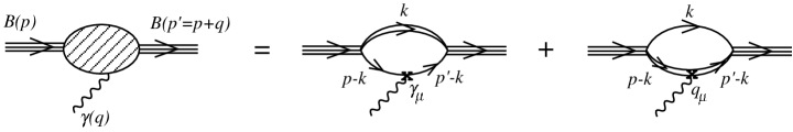
Figure 2: The Feynman diagrams for the electromagnetic coupling which generate the nucleon electromagnetic vertex.

electromagnetic field through either the quark or the diquark propagators. For the Ward-Takahashi identity to be satisfied, the wave-function renormalization $Z$ must be equal to $Z_{1}$ where $Z_{1}$ is the electromagnetic vertex renormalization constant at $q^{2}=0$. Here, $q=p^{\prime}-p$ (incoming photon) is the momentum transfer. This condition is indeed satisfied for both the Pauli-Villars and the three-momentum cut-off methods. By calculating these diagrams at an arbitrary value of momentum transfer, we derive the nucleon form factors from which we can extract the electromagnetic radii and anomalous magnetic moments.

III.4 Nucleon axial-vector vertex and the Goldberger-Treiman relation

We are in a position to calculate the weak-interaction axial-vector vertex (Fig. 3) to

Figure 3: The Feynman diagram for the axial-vector coupling which generates the quark contribution to the nucleon weak-interaction vertex.

determine the axial-vector form factors from which we can extract the axial-vector coupling constant $g_{A}$. The $g_{A}$ is defined as the coefficient of the $\gamma^{\mu}\gamma^{5}$ term of the axial-vector vertex at vanishing momentum transfer. This vertex leads naturally to the Goldberger-Treiman relation as can be seen by noticing that

$$\vec{\mathcal{A}}^{\pi}_{\mu}(\Phi)=\frac{1}{F_{\pi}}\;\partial_{\mu}\vec{\Phi}\;+\;{\cal O}(\Phi^{3})\;.$$ (34)

Thus we obtain the following term for the pion-nucleon coupling:

$$g_{A}\;\bar{B}\;\gamma^{\mu}\gamma^{5}\frac{\vec{\tau}}{2}\cdot\vec{\mathcal{A}}^{\pi}_{\mu}\;B\;\longrightarrow\;\frac{g_{A}}{F_{\pi}}\;\bar{B}\;\gamma^{\mu}\gamma^{5}\frac{\vec{\tau}}{2}\cdot\partial_{\mu}\vec{\Phi}\;B\;.$$ (35)

But this term has to be identified with the pseudovector form of the Yukawa pion-nucleon coupling Serot and Walecka (1986): $\frac{g_{\Phi NN}}{2M_{B}}\;\bar{B}\>\gamma^{\mu}\gamma^{5}{\vec{\tau}}\cdot\partial_{\mu}\vec{\Phi}\;B$, which prompts us to conclude that

$$g_{\Phi NN} = \frac{M_{B}}{F_{\pi}}g_{A}\;.$$ (36)

This is nothing but the Goldberger-Treiman relation at the composite hadron level. Note that this relation appears intact with no effort in our treatment as opposed to large violations of up to 30% in the Bethe-Salpeter equation approach Hellstern et al. (1997).

Finally, one must mention that in addition to the weak-gauge-boson coupling through the quark line (Fig. 3), there is, only for the case of the axial-vector diquark, a weak coupling through the diquark line. The quantitative contribution of this diquark to the Goldberger-Treiman relation remains to be investigated in a future work.

IV Numerical study

Having thus far derived the structure of the problem, we proceed to generate numerical results for our model using the simpler case of only scalar diquarks, thereby admitting the possibility of an intrinsic diquark form factor. Including only scalar diquarks is not out of place. Indeed, recent studies using scalar diquarks have reported good results for most of the nucleon observables Hellstern and Weiss (1995); Keiner (1996a); Hellstern et al. (1997). Moreover, there are indications of scalar diquark dominance in the nucleon Cahill et al. (1987); Reinhardt (1990); Vogl (1990). As a matter of fact, a very recent calculation using the Faddeev equation for three quark states has concluded that axial-vector correlations, while still important for magnetic properties, contribute at most no more than 10% to the structure of the nucleon Mineo et al. (2002).

IV.1 Free parameters and basic quantities

Tab. 1 provides the basic quantities in our model.

Table 1: Basic quantities in our model: The basic quantities in the microscopic model are the constituent quark mass ($m_{q}$), the scalar diquark mass ($M_{S}$), the cut-off $\Lambda$, and the quark-diquark coupling constant $\tilde{G}$.

$m_{q}$	$M_{S}$	$\Lambda$	$\tilde{G}$
$.390$ GeV	$.600$ GeV	$.630$ GeV	$271.0$ GeV-1

As for free parameters, we have first the NJL coupling constant $G$ and the NJL cut-off $\Lambda$ which are fixed to yield the constituent quark mass (quark condensate) through the NJL gap equation in the meson sector Ebert and Reinhardt (1986); Hatsuda and Kunihiro (1994); Ebert et al. (1994). In this fashion, the $G$ constant decouples completely from the nucleon sector, the sector of our interest. The two diquark masses are also determined, in a consistent manner, using the NJL model and the Bethe-Salpeter equation in the diquark channelsVogl and Weise (1991); Cahill et al. (1987). In this context, the diquark masses are simply poles, just as mesons, but in the quark-quark $T$ matrix. This leaves us with only one new free parameter in our model: the quark-diquark coupling constant $\tilde{G}$. As can be discerned, this model is well-constrained and yields a powerful predictive strength. It has to be remarked here that in principle there is another free parameter in the model : $\theta$ as the mixing angle for the two diquark contributions. But this angle has no effect in the present analysis as we consider only scalar diquarks ($\theta=0$). Moreover, one must mention that while the quark and diquark masses and the cut-off $\Lambda$ are in principle fixed through the NJL model, small variations in their values are permissible as they still lead to consistent results within the NJL model. This adds a margin of freedom to these masses.

IV.2 Nucleon static properties

Tab. 2 displays our predictions for some of the static properties of the nucleon. Experimental values are taken from Ref. Dumbrajs et al. (1983); Groom et al. (2000). A mass of 0.94 GeV is obtained for the nucleon through the mass equation Eq. (32). By fixing the nucleon mass at this value, we would have eliminated the $\tilde{G}$ coupling constant from the problem and reached a theory with no more free parameters. As for the binding energy of the nucleon, it is estimated ($m_{q}=0.390$ GeV and $M_{S}=0.600$ GeV) as $\Delta E_{\text{bin}}\equiv m_{q}+M_{S}-M_{B}=50$ MeV, suggesting that the nucleon is a loosely bound state of a quark and a diquark. This prediction is consistent with other approaches of the NJL model Hellstern and Weiss (1995) or using the Faddeev equation Ishii et al. (1993b).

Table 2: Model predictions: Some of the nucleon static properties as predicted in the present calculation using the intrinsic diquark form factor (IDFF) or without it. Experimental values are taken from Ref. Dumbrajs et al. (1983); Groom et al. (2000).

	$\mu_{p}$	$\mu_{n}$	$g_{A}$	$<r^{2}>^{p}_{E}$	$<r^{2}>^{n}_{E}$	$<r^{2}>^{p}_{M}$	$<r^{2}>^{n}_{M}$
				(fm2)	(fm2)	(fm2)	(fm2)
Theory with IDFF	1.57	-.75	.87	.77	-.11	.82	.84
Theory without IDFF	1.57	-.75	.87	.68	-.19	.82	.85
Experiment	2.79	-1.91	1.26	.74	-.12	.74	.77

In the same table, we show the magnetic moments of the proton and the neutron. Our treatment predicts a number that is two-third of the experimental value for the proton and about one-half of that for the neutron. This is not a surprising result considering that we have not included the axial-vector diquark in the present calculation. Constituent quark models and other more sophisticated approaches predict precisely that the axial-vector diquark inclusion should add the missing one-third strength to the proton and the missing one-half one to the neutron Hellstern and Weiss (1995); Keiner (1996a). So in this context, this result is exactly what one should have expected from our current analysis. For the same reason, the predicted value for the axial-vector coupling $g_{A}$ of $0.87$ is significantly less than the experimental one of $1.26$. While the scalar diquark cannot couple to the weak interaction, the axial-vector one indeed does couple to the weak gauge bosons adding strength to the interaction. The magnetic moments and the axial-vector coupling constant display a rather small sensitivity to the coupling constant $\tilde{G}$. In fact the calculated values for the magnetic moments are not that different from the predictions based on simple additive models Hellstern and Weiss (1995) suggesting a rather independence from the details of the dynamics or the nucleon size.

Speaking of the nucleon size, it is nicely well-produced by our model: the electric and magnetic radii for the proton and the neutron are close to the experimental measurements. The negative charge radius of the neutron has been suggested as an indication of a scalar diquark clustering in the nucleon Dziembowski et al. (1981), and our treatment manifests this conjecture in a dynamical model. These numbers point to a physical picture of a “heavy” diquark at the center with a quark rotating around it. By comparing the radii as calculated with and without the intrinsic diquark form factor, we find that the extended size of the diquark contributes a positive value of about $0.10~{}\text{fm}^{2}$ for each of the proton and neutron electric radii. Note that the scalar diquark has a positive charge and thus the contribution is positive adding about $0.10~{}\text{fm}^{2}$ to the proton radius and reducing the absolute value of the neutron one by the same amount. We conclude here that the size of the diquark contributes about 10% of the proton radius and 40% of the neutron one. This confirms an earlier calculation using a static quark-exchange approximation Hellstern and Weiss (1995). As anticipated, the intrinsic form factor has virtually no effect on the magnetic radii as the scalar diquark, as we shall see below, has a negligible contribution to the magnetic form factors. Moreover, we have found the electromagnetic radii to be very sensitive to the binding energy as well as, although implicitly through the mass equation (Eq.( 32)), the coupling constant $\tilde{G}$. This indicates, as easily expected, the importance of the details of the dynamics for the nucleon size. We should remark here that the quantities calculated here do not contain the pion contribution which becomes significant for some physical quantities. It is estimated that for $m_{\pi}=138$ MeV, typical values for the pion corrections are of order of 30%.

IV.3 Nucleon electric and magnetic form factors

Next we calculate the nucleon form factors. Fig. 4 displays the proton electric form factor in comparison with experimental data taken from Ref. Höhler et al. (1976). The figure shows the quark contribution, the diquark contribution in addition to the full form factor (the sum of the two contributions), with no intrinsic diquark form factor.

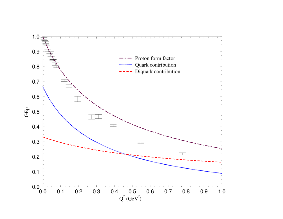
Figure 4: The proton electric form factor in comparison with experimental data. The figure shows the quark contribution (dotted line), the diquark contribution (dashed line) as well as the full form factor (dotted-dashed line) as the sum of the two contributions. Intrinsic structure of the scalar diquark is not included here. Experimental data from Ref. Höhler et al. (1976) are included.

It is evident that our treatment reproduces beautifully the form factor at low values of momentum transfer ($Q^{2}\equiv-q^{2}$ where $q$ is the momentum transfer). The discrepancy at higher values of $Q^{2}$ begs for an understanding. The figure suggests an explanation: the diquark contribution is almost constant implying a rather localized diquark inside the proton. Although treated as an elementary field in our theory, the diquark is a composite object and does have a finite size. Our treatment needs to be adjusted to reflect the true nature of the diquark by incorporating an intrinsic diquark form factor. Fortunately, diquark form factors have been calculated recently and in fact in the framework of the NJL model Weiss et al. (1993). Thus we readily add the intrinsic diquark form factor to our treatment and produce the proton form factor shown in Fig. 5. Impressively, the calculations matches very well with the experimental data.

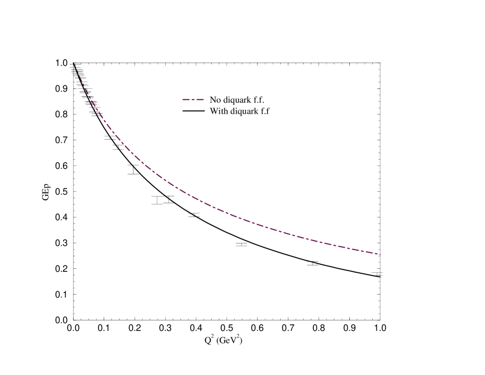
Figure 5: The proton electric form factor, with intrinsic diquark form factor (diquark f.f.), in comparison with experimental data. The figure shows the form factor with no intrinsic diquark form factor (dotted-dashed line), and with the intrinsic form factor (solid line). Experimental data from Ref. Höhler et al. (1976) are included.

The neutron electric form factor tells a similar story. In the left panel of Fig. 6, just as in Fig. 4, we display the neutron

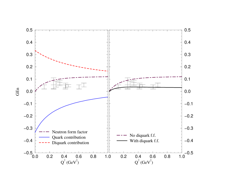
Figure 6: The neutron electric form factor in comparison with experimental data. The left panel shows the quark contribution (dotted line), the diquark contribution (dashed line) as well as the full form factor (dotted-dashed line) as the sum of the two contributions. The right panel displays the neutron form factor with no intrinsic diquark form factor (dotted-dashed line), and with the intrinsic form factor (solid line). Experimental data from Ref. Eden et al. (1994); Bruins et al. (1995); Ostrick et al. (1999); Rohe et al. (1999); Zhu et al. (2001) are included.

form factor with its quark and diquark contributions. Clearly, the quark contribution is negative in value (d-quark) and thus cancels much of the diquark contribution leading to a small form factor. There is once more a discrepancy compared to experimental data that is largely eliminated once we include the intrinsic form factor as exhibited in the right panel of the same figure. It is noteworthy here that the neutron form factor is a potent test of any treatment as it is a delicate cancellation of two large contributions Keiner (1996a, b). Saliently, the cancellation is naturally produced in our study. The experimental data are obtained from Ref. Eden et al. (1994); Bruins et al. (1995); Ostrick et al. (1999); Rohe et al. (1999); Zhu et al. (2001).

In Fig. 7, we present the proton magnetic form factor as calculated with or without the intrinsic diquark form factor. The figure also contains the quark and diquark contributions. Unmistakably, the scalar diquark contribution is virtually vanishing due to the lack of an intrinsic spin. Nevertheless, there is a very small contribution due to a small orbital angular-momentum effect in the bound quark-diquark system. Since the diquark contribution is negligible, the inclusion of the intrinsic diquark form factor does not alter our prediction and the form factor is determined to be almost purely from a quark origin. This suggests the need for the axial-vector diquark, which does have an intrinsic spin, to supplement the quark contribution and to provide the missing one-third strength compared to the experimental data Höhler et al. (1976). The figure also indicates a convergence of our calculation, mainly from a quark origin, and the experimental data at large values of $Q^{2}$. Such result suggests that this form factor is almost purely from a quark origin in this regime. This is anticipated due to the finite size of the axial-vector diquark which probably can have a significant contribution but only for smaller values of $Q^{2}$.

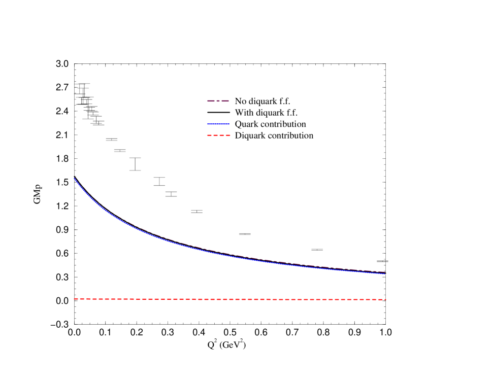
Figure 7: The proton magnetic form factor in comparison with experimental data. The figure shows the proton magnetic form factor as calculated with (solid line) or without (dotted-dashed line) the intrinsic diquark form factor. The figure also includes the quark (dotted line) and the diquark (dashed line) contributions to this form factor. Note that the three curves (apart form the diquark contribution) are very similar. Experimental data from Ref. Höhler et al. (1976) are included.

The neutron magnetic form factor describes a similar narrative to that of the proton but here the missing strength (one-half) is larger as can be seen in Fig. 8. As stated earlier, these specific missing strengths are predicted due to the absence of the axial-vector diquark in the present analysis. The experimental data in Fig. 8 are obtained from Ref. Anklin et al. (1994); Bruins et al. (1995); Anklin et al. (1998); Golak et al. (2001); Xu et al. (2000); Kubon et al. (2002).

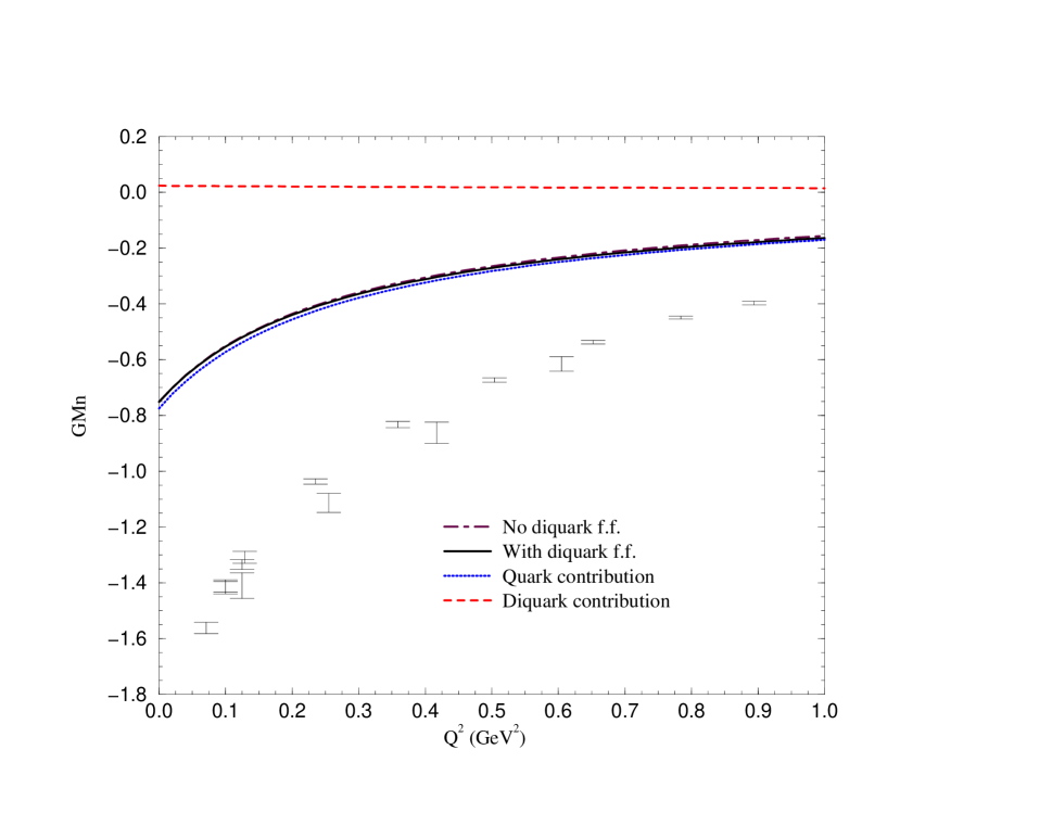
Figure 8: The neutron magnetic form factor in comparison with experimental data. The figure shows the neutron magnetic form factor as calculated with (solid line) or without (dotted-dashed line) the intrinsic diquark form factor. The figure also includes the quark (dotted line) and the diquark (dashed line) contributions to this form factor. Note that the three curves (apart form the diquark contribution) are very similar. Experimental data from Ref. Anklin et al. (1994); Bruins et al. (1995); Anklin et al. (1998); Golak et al. (2001); Xu et al. (2000); Kubon et al. (2002) are included.

V Conclusions

In this paper we tackled the nucleon structure and the challenging problem of understanding the origin and nature of the nuclear force by deriving a meson-nucleon Lagrangian using the path-integral method of hadronization. We started from a microscopic model of quarks and diquarks where the gluonic degrees of freedom have been integrated out. The nucleon was conceived as quark-diquark correlations and only two kinds of diquarks were found relevant for its structure. These are the scalar isoscalar and the axial-vector isovector diquarks. Composite meson and nucleon fields were introduced by the methods of path-integral bosonization and fermionization to rewrite the problem in terms of the physical meson and nucleon degrees of freedom. This yielded an effective chiral meson-nucleon Lagrangian after using a loop and derivative expansions of the resulting quark/diquark determinants. The divergent loop diagrams were regularized using gauge-invariant regularization schemes and the Ward-Takahashi identity and the Goldberger-Treiman relation were verified.

An extensive set of nucleon observables were calculated for the first time on the basis of the path-integral hadronization approach. Indeed, many of the nucleon physical properties such as mass, coupling constants, electromagnetic radii, anomalous magnetic moments, and form factors have been determined from a model of essentially one free parameter. By taking into account the intrinsic diquark form factor, we established a remarkable agreement with the experimental data for the nucleon size and the electric form factors, while our calculations show missing strengths for the magnetic form factors and the axial-vector coupling constant. The discrepancy is likely due to the absence of the axial-vector diquark in the present numerical study.

This work is part of an ambitious program of using path-integral techniques and QCD-based effective field theories to study baryon structure and to derive a full-fledged nuclear force. The final goal of the program is a derivation of an effective field theory for the nuclear force, namely, quantum hydrodynamics (QHD) from quark dynamics. As for the future, we plan to attain a numerical study using both the scalar and axial-vector diquarks including their intrinsic form factors . This is a challenging and rather difficult task due to the axial-vector diquark intricate structure as a particle of one unit spin and isospin. Some of the ensuing complications are the axial-vector diquark direct coupling to the weak interaction and the electroweak scalar-axial-vector transitions. At a later stage, we plan to generalize our approach to chiral SU(3) symmetry to study the structure of the baryon octet.

*

Appendix A Analytical expressions using the Pauli-Villars regularization method

We include here analytical expressions for some of the principal formulae in our treatment.

A.1 Self-energy and wave-function renormalization

The self-energy is depicted by the Feynman diagram of Fig. 1 and is given by the expression:

$$\Sigma(p) = N_{c}\;(-i)\int\frac{d^{4}k}{(2\pi)^{4}}\;\frac{i\left(\hbox to0.0pt{/\hss}p-\hbox to0.0pt{/\hss}k+m_{q}\right)}{(p-k)^{2}-m_{q}^{2}}\;\left[\frac{i}{k^{2}-M_{S}^{2}}-\frac{i}{k^{2}-\Lambda^{2}}\right]\;,$$ (37)

$$= N_{c}\;\frac{1}{(4\pi)^{2}}\int^{1}_{0}dx\;\left[\hbox to0.0pt{/\hss}p(1-x)+m_{q}\right]\;\ln\left[\frac{\Delta(\Lambda,q^{2}=0)}{\Delta(M_{S},q^{2}=0)}\right]\;.$$

Here $p^{\mu}$ is the momentum of the nucleon taken to be on the mass shell, $N_{c}=3$ is the number of colors, and

$$\Delta(M,q^{2})\equiv m_{q}^{2}x+M^{2}(1-x)-p^{2}x(1-x)+q^{2}x^{2}y(y-1)\;.$$ (38)

Note that we have used the Pauli Villars method for regularizing the divergent integral by incorporating the propagator $\frac{i}{k^{2}-\Lambda^{2}}$ of a fictitious scalar particle with mass $\Lambda$ in the above expression.

The wave-function renormalization $Z$ is obtained through the derivative $\frac{\partial\Sigma(p)}{\partial p_{\mu}}{\bigg{|}}_{\hbox to0.0pt{/\hss}p\rightarrow M_{B}}$, leading to the expression:

$$Z^{-1} = N_{c}\;\frac{1}{(4\pi)^{2}}\int^{1}_{0}dx\;\bigg{\{}\;(1-x)\ln\left[\frac{\Delta(\Lambda,q^{2}=0)}{\Delta(M_{S},q^{2}=0)}\right]-$$ (39)

$$2x(1-x)\>M_{B}\>\left[M_{B}(1-x)+m_{q}\right]\;\left[\frac{1}{\Delta(\Lambda,q^{2}=0)}-\frac{1}{\Delta(M_{S},q^{2}=0)}\right]\;\bigg{\}}\;.$$

A.2 Electromagnetic interaction

The photon couples to both the quark and the diquark lines leading to two contributions to the nucleon electromagnetic vertex.

A.2.1 Quark contribution

This is the contribution represented by the left part of Fig. 2 and is given by:

$$-\Lambda^{\mu}_{\gamma q} = -\;N_{c}\;Q_{q}\;\int\frac{d^{4}k}{(2\pi)^{4}}\;\left[\frac{i}{k^{2}-M_{S}^{2}}-\frac{i}{k^{2}-\Lambda^{2}}\right]\frac{i\left(\hbox to0.0pt{/\hss}p^{\prime}-\hbox to0.0pt{/\hss}k+m_{q}\right)}{(p^{\prime}-k)^{2}-m_{q}^{2}}\;\gamma^{\mu}\;\frac{i\left(\hbox to0.0pt{/\hss}p-\hbox to0.0pt{/\hss}k+m_{q}\right)}{(p-k)^{2}-m_{q}^{2}}\;,$$ (40)

$$= F_{1}^{q}(q^{2})\;\gamma^{\mu}+F_{2}^{q}(q^{2})\;\frac{i\sigma^{\mu\nu}\>q_{\nu}}{2M_{B}}\;,$$

where $F_{1}^{q}(q^{2})$ and $F_{2}^{q}(q^{2})$ are the quark contributions to the nucleon form factor and are given by:

$$F_{1}^{q}(q^{2}) = Z\;N_{c}\;Q_{q}\;\frac{1}{(4\pi)^{2}}\;\int^{1}_{0}dx\int^{1}_{0}dy\;\;\bigg{\{}\;(1-x)\ln\left[\frac{\Delta(\Lambda,q)}{\Delta(M_{S},q)}\right]-$$

$$\bigg{[}2x(1-x)M_{B}\>\left[M_{B}(1-x)+m_{q}\right]+q^{2}x^{2}(1-y)\bigg{]}\left[\frac{1}{\Delta(\Lambda,q)}-\frac{1}{\Delta(M_{S},q)}\right]\;\bigg{\}}\;,$$

$$F_{2}^{q}(q^{2}) = Z\;N_{c}\;Q_{q}\;\frac{1}{(4\pi)^{2}}\;\int^{1}_{0}dx\int^{1}_{0}dy\;\;$$

$$\hskip 71.13188pt\;\times\;2x^{2}M_{B}\>\left[M_{B}(1-x)+m_{q}\right]\;\left[\frac{1}{\Delta(\Lambda,q)}-\frac{1}{\Delta(M_{S},q)}\right]\;\;.$$ (42)

In the above expressions, $p^{\mu}$ ($p^{\prime\mu}$) is the momentum of the incoming (outgoing) nucleon, $q^{\mu}=p^{\prime\mu}-p^{\mu}$ is the momentum transfer, and $Q_{q}=\text{diag}\left(2/3,-1/3\right)$ is the quark charge. Note that we have included the wave-function renormalization constant $Z$ in the above expressions.

A.2.2 Scalar diquark contribution

This is the contribution represented by the right part of Fig. 2 and is given by:

$$-\Lambda^{\mu}_{\gamma D} = -\;N_{c}\;Q_{S}\;\int\frac{d^{4}k}{(2\pi)^{4}}\;\bigg{\{}\frac{i}{(p-k)^{2}-M_{S}^{2}}\;\frac{i\left(\hbox to0.0pt{/\hss}k+m_{q}\right)}{k^{2}-m_{q}^{2}}\;\frac{i}{(p^{\prime}-k)^{2}-M_{S}^{2}}-$$ (43)

$$\hskip 56.9055pt\frac{i}{(p-k)^{2}-\Lambda^{2}}\;\frac{i\left(\hbox to0.0pt{/\hss}k+m_{q}\right)}{k^{2}-m_{q}^{2}}\;\frac{i}{(p^{\prime}-k)^{2}-\Lambda^{2}}\;\bigg{\}}\;\left(p^{\mu}-p^{\prime\;\mu}-2k^{\mu}\right)\;,$$

$$= F_{1}^{D}(q^{2})\;\gamma^{\mu}+F_{2}^{D}(q^{2})\;\frac{i\sigma^{\mu\nu}\>q_{\nu}}{2M_{B}}\;,$$

where

$$F_{1}^{D}(q^{2}) = ZN_{c}\;Q_{S}\;\frac{1}{(4\pi)^{2}}\;\int^{1}_{0}dx\int^{1}_{0}dy\;\;\bigg{\{}\;(1-x)\ln\left[\frac{\Delta(\Lambda,q)}{\Delta(M_{S},q)}\right]-$$ (44)

$$\bigg{[}2x(1-x)M_{B}\>\left[M_{B}(1-x)+m_{q}\right]\bigg{]}\left[\frac{1}{\Delta(\Lambda,q)}-\frac{1}{\Delta(M_{S},q)}\right]\;\bigg{\}}\;,$$

$$F_{2}^{D}(q^{2}) = ZN_{c}\;Q_{S}\;\frac{1}{(4\pi)^{2}}\;\int^{1}_{0}dx\int^{1}_{0}dy\;\;\bigg{\{}$$

$$\hskip 28.45274pt\;2x(1-x)M_{B}\>\left[M_{B}(1-x)+m_{q}\right]\;\left[\frac{1}{\Delta(\Lambda,q)}-\frac{1}{\Delta(M_{S},q)}\right]\;\bigg{\}}\;.$$ (45)

Here $Q_{S}=1/3$ is the diquark charge.

A.2.3 Form factor and Ward-Takahashi identity

The full nucleon electromagnetic form factor is the sum of the quark and diquark contributions. Note that at $q^{2}=0$, the sum of these two pieces conforms to the Ward-Takahashi identity as it yields $Z\>\left(Q_{q}+Q_{S}\right)\>\frac{1}{Z}=\text{diag}\left(1,0\right)=Q_{N}$ with the correct normalization for the nucleon electric charge.

A.3 Axial-vector coupling constant $g_{A}$

The axial-vector coupling constant $g_{A}$ (with only scalar diquarks) is determined from the axial-vector vertex as represented by Fig 3. Note that since the scalar diquark cannot couple to the weak interaction, there is no contribution to $g_{A}$ from a direct coupling to the diquark line. The full axial-vector vertex is given by:

$${\mathcal{A}}^{\mu}_{\text{axial}} = -\;N_{c}\;\int\frac{d^{4}k}{(2\pi)^{4}}\;i\left[\frac{i}{k^{2}-M_{S}^{2}}-\frac{i}{k^{2}-\Lambda^{2}}\right]\frac{i\left(\hbox to0.0pt{/\hss}p^{\prime}-\hbox to0.0pt{/\hss}k+m_{q}\right)}{(p^{\prime}-k)^{2}-m_{q}^{2}}\;\gamma^{\mu}\gamma^{5}\;\frac{i\left(\hbox to0.0pt{/\hss}p-\hbox to0.0pt{/\hss}k+m_{q}\right)}{(p-k)^{2}-m_{q}^{2}}\;.$$

The $g_{A}$ is defined as the coefficient of the $\gamma^{\mu}\gamma^{5}$ term of the axial-vector vertex at $q^{2}=0$. This yields after evaluating this vertex

$$g_{A} = -Z\;N_{c}\;\frac{1}{(4\pi)^{2}}\;\int^{1}_{0}dx\int^{1}_{0}dy\;\;\bigg{\{}\;x\ln\left[\frac{\Delta(\Lambda,q^{2}=0)}{\Delta(M_{S},q^{2}=0)}\right]-$$ (47)

$$\hskip 59.75095ptx\>\left[M_{B}(1-x)+m_{q}\right]^{2}\left[\frac{1}{\Delta(\Lambda,q^{2}=0)}-\frac{1}{\Delta(M_{S},q^{2}=0)}\right]\;\bigg{\}}\;.$$