Unitarity and the Bethe-Salpeter Equation

Abstract

We investigate the relation between different three-dimensional reductions of the Bethe-Salpeter equation and the analytic structure of the resultant amplitudes in the energy plane. This correlation is studied for both the $\phi^{2}\sigma$ interaction Lagrangian and the $\pi N$ system with $s$-, $u$-, and $t$-channel pole diagrams as driving terms. We observe that the equal-time equation, which includes some of the three-body unitarity cuts, gives the best agreement with the Bethe-Salpeter result. This is followed by other 3-D approximations that have less of the analytic structure.

I Introduction

The interest in pion-nucleon ($\pi N$) scattering has shifted in recent years from low energies to energies near and above the pion production threshold. This has been motivated by the growing importance of the low energy baryon spectrum, and in particular the $N^{*}(1440)$ and $N^{*}(1535)$ in the study of QCD models. At these energies one needs to make use of a relativistic formulation of $\pi N$ scattering, with the Bethe-Salpeter (BS) equation Salpeter and Bethe (1951) being a prime candidate. The problem here is that the BS equation is four-dimensional, with a kernel that has a complex analytic structure. This has inspired a number of three-dimensional reductions to the BS equation that have been employed in meson-exchange models of $\pi N$ and nucleon-nucleon ($NN$) scattering. In fact, it has been established that one can generate an infinity of such equations that satisfy two-body unitarity Klein and Lee (1974). The question that is often raised is which of these equations is the optimum one to be used for a given problem. To define such an optimum equation one needs criteria for the definition of optimum.

One such criterion proposed by Gross Gross (1982) stated that any relativistic two-body equation should have the correct one-body limit, i.e., in the limit as one of the masses goes to infinity the equation reduces to either the Dirac or Klein-Gordon equation. The Gross equation Gross (1982) achieves this limit by placing one of the particles on-mass-shell. This effectively reduces the BS equation to a 3-D equation, and in the ladder approximation has the correct one-body limit. The full BS equation does satisfy the one-body limit, but the ladder BS equation fails to satisfy this condition. This could be partly remedied in $NN$ scattering by including the crossed as well as the ladder graphs in the kernel of the BS equation Mandelzweig and Wallace (1987); Wallace and Mandelzweig (1989); Phillips and Wallace (1996). For $\pi N$ scattering it is not clear as to how one may impose the one-body limit short of resorting to the inclusion of the crossed-ladder diagrams. Placing the pion on-shell Gross and Surya (1993) may be the optimal solution for iterating the $u$-channel pole diagrams, but is not as good for the $t$-channel pole diagrams Pascalutsa (1995); Pascalutsa and Tjon (1999).

An alternative scheme for developing relativistic 3-D equations that avoids the above ambiguities of the 3-D reductions, and is a natural extension of the non-relativistic two-body scattering problem, is based on a formulation of scattering theory using the generators of the Poincaré group Bakamjian and Thomas (1953); Keister and Polyzou (1991). This formulation, which introduces the interaction through one of the generators of the group, satisfies two-body unitarity and can be extended to include three-body unitarity. Recently, Fuda Fuda (1995); Elmessiri and Fuda (1998) has adapted this approach to the $\pi N$ system within the framework of the coupled channel approach satisfying two-body unitarity only. To establish the connection with meson exchange models Elmessiri and Fuda (1999), the mass operator $M$ in the interacting system is related to the mass operator in the free system ($M_{0}$) by the linear relation $M=M_{0}+U$ in which $U$ is the interaction. This interaction is defined on the Hilbert space of baryon ($B$) and meson-baryon ($mB$) states, allowing for the coupling between the two channels. To remove the energy dependence of the meson exchange potentials they resort to Okuba’s Ohkuba (1954) unitary transformation. The source of ambiguities in this approach are: (i) the choice for the Poincaré generator in which the interaction is introduced, and (ii) the method by which the energy dependence is removed from the interaction.

In the present analysis we propose to examine a third alternative to the reduction of the BS equation from a four-dimensional to a three-dimensional integral equation. Here we are motivated by trying to preserve as much as possible the unitarity content of the BS equation while preserving the two-body nature of the integral equation. This is partly a result of the observation that the low energy resonances observed in $\pi N$ scattering are near the three-body threshold, and one may need more than just two-body unitarity. It also could form the starting point of a three-body formulation of $\pi N$ scattering without the complexity of the three-particle BS equation.

To examine the importance of the role of unitarity in the reduction of the BS equation, we examine a small class of three-dimensional equations that preserve some of the unitarity cuts in the BS equation. In particular, we consider the the Klein Klein (1953) or “equal-time” (ET) equation Phillips and Wallace (1996); Lahiff and Afnan (1997), the Cohen (C) approximation Cohen (1970), the instantaneous (I) approximation Salpeter (1952); Mandelzweig and Wallace (1987); Wallace and Mandelzweig (1989); Pascalutsa and Tjon (2000) used recently by Pascalutsa and Tjon for $\pi N$ scattering Pascalutsa and Tjon (2000), and the Blankenbecler-Sugar (BbS) equation Blankenbecler and Sugar (1966). Since there are an infinite number of possible 3-D equations, there are many other equations that we could compare to the BS equation. However, we have chosen to consider only a small set of equations which differ in the analytic structure of the resultant amplitude in the energy or $\sqrt{s}$-plane.

In Sec. II we first examine the analytic structure of the BS amplitude for $\phi\phi$ scattering in the $\phi^{2}\sigma$ model by performing a pinch analysis Pagnamenta and Taylor (1966) on the relative energy integration in the kernel of the integral equation. We will find in this simple model that as we proceed from the BS equation to the ET, Cohen, and finally to the instantaneous equation and the BbS equation, we are including less and less of the analytic structure present in the original BS amplitude. We then in Sec. III proceed to present the results of the same analysis for $\pi N$ scattering, within the framework of $s$-, $u$- and $t$-channel exchange potentials. To illustrate the magnitude and effect of these thresholds for both $\phi\phi$ and $\pi N$ scattering, we present in Sec. IV numerical results for both models over the region covering the lowest three-body thresholds. Finally, in Sec. V we give some concluding remarks regarding the 3-D approximations to the BS equation.

II Analytic Structure of the Scattering Amplitude

Unlike two-body equations in three dimensions, the BS equation generates unitarity thresholds by the pinching of relative energy integration contour by the poles and branch points of the integrand of the integral equation. To illustrate this, we consider a simple model in which the interaction Lagrangian is $g\phi^{2}\sigma$, where $g$ is the strength of the interaction, while $\phi$ and $\sigma$ are the two scalar fields in the model. We will further assume that the kernel of the BS equation for $\phi\phi$ scattering is approximated by one $\sigma$-exchange. The motivation for this approximation is to simplify the analysis while maintaining the main features of $NN$ scattering in terms of $t$-channel exchange, and $\pi N$ scattering in terms of $s$-, $u$- and $t$-channel exchanges.

The BS equation for $\phi\phi$ scattering, after partial wave expansion, is a two-dimensional integral equation of the form

$$T_{\ell}(\hat{q},\hat{q}^{\prime};s)=V_{\ell}(\hat{q},\hat{q}^{\prime};s)-i\int_{-\infty}^{\infty}dq^{\prime\prime}_{0}\ \int_{0}^{\infty}dq^{\prime\prime}V_{\ell}(\hat{q},\hat{q}^{\prime\prime};s)\,G(\hat{q}^{\prime\prime},s)\,T_{\ell}(\hat{q}^{\prime\prime},\hat{q}^{\prime};s)\ ,$$ (1)

where $\hat{q}=(q_{0},q)$ is the zero component and magnitude of the space component of the relative momentum, while $P=k_{1}+k_{2}=(\sqrt{s},\textbf{0})$ is the total four-momentum in the center of mass. Although there are several definitions for the relative four-momentum Pearce and Jennings (1991), the most convenient, from the point of view of the Wick rotation Wick (1954), is $q=\frac{1}{2}(k_{1}-k_{2})$. For scalar particles, the two-body propagator in the center of mass is

$$G(\hat{q},s)=\left[\left(\frac{1}{2}\sqrt{s}+q_{0}\right)^{2}-E^{2}_{q}+i\epsilon\right]^{-1}\ \left[\left(\frac{1}{2}\sqrt{s}-q_{0}\right)^{2}-E^{2}_{q}+i\epsilon\right]^{-1}\ ,$$ (2)

where $E_{q}=\sqrt{q^{2}+m^{2}}$, with $m$ the mass of the $\phi$ particle. The partial wave potential due to the exchange of a $\sigma$ particle of mass $\mu$ is given by

$$V_{\ell}(\hat{q},\hat{q}^{\prime};s)=\frac{g^{2}}{(2\pi)^{3}}\,Q_{\ell}\left(\frac{(q_{0}-q^{\prime}_{0})^{2}-q^{2}-{q^{\prime}}^{2}-\mu^{2}+i\epsilon}{-2qq^{\prime}}\right)\ .$$ (3)

Here $Q_{\ell}$ is the Legendre function of the second kind, and for $\ell=0$ this potential takes the form

$$V_{0}(\hat{q},\hat{q}^{\prime};s)=\frac{g^{2}}{2(2\pi)^{3}}\ \log\left(\frac{(q_{0}-q^{\prime}_{0})^{2}-\omega^{2}_{q+q^{\prime}}+i\epsilon}{(q_{0}-q^{\prime}_{0})^{2}-\omega^{2}_{q-q^{\prime}}+i\epsilon}\right)\ ,$$ (4)

where $\omega_{p}=\sqrt{p^{2}+\mu^{2}}$. This form exhibits the logarithmic branch points of the potential. We observe that the potential is independent of the total energy squared, $s$.

The analytic structure of the partial wave amplitude in the energy ($\sqrt{s}$) plane is determined by the pinching of the $q^{\prime\prime}_{0}$ integration contour by the singularities of the integrand Eden (1952, 1962). These singularities arise from the potential $V_{\ell}(\hat{q},\hat{q}^{\prime\prime};s)$, the two-body propagator $G(\hat{q}^{\prime\prime},s)$, and the scattering amplitude $T_{\ell}(\hat{q}^{\prime\prime},\hat{q}^{\prime};s)$. The two-body propagator has four poles in the $q^{\prime\prime}_{0}$-plane. These poles, labelled $1)\dots 4)$, are located at

$$1)\quad q^{\prime\prime}_{0} = -\frac{1}{2}\sqrt{s}-E_{q^{\prime\prime}}+i\epsilon\quad;\quad 2)\quad q^{\prime\prime}_{0}=\frac{1}{2}\sqrt{s}-E_{q^{\prime\prime}}+i\epsilon\ ;$$

$$3)\quad q^{\prime\prime}_{0} = -\frac{1}{2}\sqrt{s}+E_{q^{\prime\prime}}-i\epsilon\quad;\quad 4)\quad q^{\prime\prime}_{0}=\frac{1}{2}\sqrt{s}+E_{q^{\prime\prime}}-i\epsilon\ ,$$ (5)

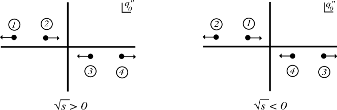
Figure 1: The poles of the two-body propagator in the $q^{\prime\prime}_{0}$-plane.

and are illustrated in Fig. 1. As we increase $\sqrt{s}>0$ the poles $1)$ and $3)$ move to the left in the $q^{\prime\prime}_{0}$-plane, while poles $2)$ and $4)$ move to the right.

To examine the conditions under which the $q^{\prime\prime}_{0}$ integration contour gets pinched by the poles in the propagator, we consider Fig. 1. Here we have to ensure that the two poles that pinch the contour of integration come from the Feynman propagators of two different particles. As a result poles $1)$ and $4)$ ( or $2)$ and $3)$ ) can pinch the contour, while $1)$ and $3)$ ( or $2)$ and $4)$ ) cannot pinch the contour as they belong to the same particle propagator. This results from the fact that while the Feynman propagator for a single particle can be decomposed into a positive and a negative energy component, these components cannot pinch the contour of integration as they cannot generate any new thresholds. We therefore have, for $\sqrt{s}>0$, the condition for the poles $2)$ and $3)$ to pinch the contour to be

$$\frac{1}{2}\sqrt{s}-E_{q^{\prime\prime}}+i\epsilon=-\frac{1}{2}\sqrt{s}+E_{q^{\prime\prime}}-i\epsilon$$ (6)

or

$$\sqrt{s}=2\,E_{q^{\prime\prime}}-2i\epsilon\ .$$ (7)

Here we note that if we deform the $q^{\prime\prime}$ contour of integration in Eq. (1), e.g. $q^{\prime\prime}\rightarrow q^{\prime\prime}\,e^{-i\phi}$, then $E_{q^{\prime\prime}}$ will acquire a negative imaginary part and as a result the $q_{0}^{\prime\prime}$ integration contour will not get pinched. This is true for all values of $q^{\prime\prime}$ except $q^{\prime\prime}=0$. Therefore we may conclude that the pinching of the $q^{\prime\prime}_{0}$ contour generates a branch point at $\sqrt{s}=2m$, which is the threshold for two-body scattering.

The same analysis can be carried through for $\sqrt{s}<0$. In this case the contour of integration in the $q^{\prime\prime}_{0}$ variable is pinched by the poles 1) and 4), with the condition for the pinch being

$$\sqrt{s}=-2\,E_{q^{\prime\prime}}+2i\epsilon\ .$$ (8)

This will generate a branch point at $\sqrt{s}=-2m$. This result establishes the fact that if we take both branch points resulting from the pinching of the integration contour by the poles of the two-body propagator, we get an amplitude that is analytic in $s$. In this way charge conjugation symmetry is preserved Pascalutsa and Tjon (1998). However, if we only include the branch point at $\sqrt{s}=2m$, then we have only a right hand cut in the $\sqrt{s}$-plane and the resultant amplitude is a function of $\sqrt{s}$, i.e., it satisfies two-body unitarity, but violates charge conjugation symmetry.

The potential $V_{\ell}(\hat{q},\hat{q}^{\prime\prime};s)$ gives rise to two pairs of logarithmic branch points in the $q^{\prime\prime}_{0}$-plane. These branch points, labelled $5)\dots 8)$, are located at

$$5)\quad q^{\prime\prime}_{0}=q_{0}-\omega_{q+q^{\prime\prime}}+i\epsilon\quad; \quad 6)\quad q^{\prime\prime}_{0}=q_{0}-\omega_{q-q^{\prime\prime}}+i\epsilon\ ;$$

$$7)\quad q^{\prime\prime}_{0}=q_{0}+\omega_{q+q^{\prime\prime}}-i\epsilon\quad; \quad 8)\quad q^{\prime\prime}_{0}=q_{0}+\omega_{q-q^{\prime\prime}}-i\epsilon\ ,$$ (9)

with branch points $5)$ and $6)$ ( $7)$ and $8)$ ) being connected by a logarithmic branch cut. These are illustrated in Fig. 2. Since the potential is due to the exchange of a scalar particle, the potential, before partial wave expansion, is proportional to the Feynman propagator for that scalar. Here again the decomposition of the propagator into positive and negative energy components gives rise to the two logarithmic cuts in Fig. 2, and each will give rise to a separate term in the multiple scattering series.

We now can examine the pinching of the contour of integration in the $q^{\prime\prime}_{0}$-plane by a combination of a propagator pole and a potential branch point. Take for example the pole 2) with the branch point 8). The condition for the pinch is

$$\frac{1}{2}\sqrt{s}-E_{q^{\prime\prime}}+i\epsilon=q_{0}+\omega_{q-q^{\prime\prime}}-i\epsilon$$ (10)

or

$$\frac{1}{2}\sqrt{s}=q_{0}+E_{q^{\prime\prime}}+\omega_{q-q^{\prime\prime}}-2i\epsilon\equiv p_{0}\ .$$ (11)

Here again contour deformation, e.g. $q^{\prime\prime}\rightarrow q^{\prime\prime}e^{-i\phi}$, will stop us from pinching the contour since both $E_{q^{\prime\prime}}$ and $\omega_{q-q^{\prime\prime}}$ acquire a finite imaginary part. The exception again is the point $q^{\prime\prime}=0$. In this case the value of $q^{\prime\prime}$ for which we get the pinching of the contour depends on $\hat{q}$. To determine the position of the branch point in the $\sqrt{s}$-plane, we need to find the minimum value of $p_{0}$ or $\sqrt{s}$ with respect to $q^{\prime\prime}$ for which we have a pinch, i.e.,

$$\frac{\partial p_{0}}{\partial q^{\prime\prime}}=\frac{q^{\prime\prime}}{E_{q^{\prime\prime}}}-\frac{(q-q^{\prime\prime})}{\omega_{q-q^{\prime\prime}}}=0\ .$$

This equation is used to determine $q^{\prime\prime}$ in terms of $q$, and gives

$$q^{\prime\prime}=\frac{m}{m+\mu}\,q\ .$$

We now can establish that the off-mass-shell scattering amplitude has a branch cut in the $q_{0}$-plane at Pagnamenta and Taylor (1966)

$$q_{0}=\frac{1}{2}\sqrt{s}-\sqrt{q^{2}+(m+\mu)^{2}}+2i\epsilon\ .$$ (12)

This gives the singularity in the relative energy $q^{\prime\prime}_{0}$ for the off-mass-shell amplitude that is being integrated over in Eq. (1).

Following the same procedure, we examine the pinching of the contour by the singularities $3)$ and $6)$ for $\sqrt{s}>0$, while for $\sqrt{s}<0$ the contour is pinched by either $1)$ and $8)$, or $4)$ and $6)$. As a result the off-mass-shell amplitude in the integral has four possible branch cuts in the $q^{\prime\prime}_{0}$-plane. These are at

$$9)\quad q^{\prime\prime}_{0}=\frac{1}{2}\sqrt{s}-{\cal E}_{q^{\prime\prime}}+2i\epsilon\ ;\quad 10)\quad q^{\prime\prime}_{0}=-\frac{1}{2}\sqrt{s}+{\cal E}_{q^{\prime\prime}}-2i\epsilon$$ (13)

for $\sqrt{s}>0$, and for $\sqrt{s}<0$ the branch cuts are given by

$$11)\quad q^{\prime\prime}_{0}=\frac{1}{2}\sqrt{s}+{\cal E}_{q^{\prime\prime}}-2i\epsilon\ ;\quad 12)\quad q^{\prime\prime}_{0}=-\frac{1}{2}\sqrt{s}-{\cal E}_{q^{\prime\prime}}+2i\epsilon\ ,$$ (14)

where ${\cal E}_{q}=\sqrt{q^{2}+(m+\mu)^{2}}$. In Fig. 3 we illustrate the positions of the corresponding branch points in the $q^{\prime\prime}_{0}$-plane. At this stage we should recall that the singularities $9)$ and $10)$ are in different terms in the multiple scattering series, and therefore cannot pinch the contour of integration as may be inferred from Fig. 3.

Since the singularities $9)\dots 12)$ are in the off-mass-shell BS amplitude, they are present in the integrand of the integral equation, Eq. (1). These singularities in the amplitude can, in conjunction with the propagator poles or potential branch points, pinch the $q^{\prime\prime}_{0}$ integration contour and generate further singularities in the amplitude on the left hand side of Eq. (1).

Let us first consider the pinching of the contour by the amplitude singularities and the propagator poles. For $\sqrt{s}>0$ we now can have the integration contour pinched by the singularities $2)$ and $10)$ ( or $3)$ and $9)$ ). The condition for the pinching between the pole $2)$ and the singularity $10)$ is

$$\frac{1}{2}\sqrt{s}-E_{q^{\prime\prime}}+i\epsilon=-\frac{1}{2}\sqrt{s}+{\cal E}_{q^{\prime\prime}}-2i\epsilon$$ (15)

or

$$\sqrt{s}=E_{q^{\prime\prime}}+{\cal E}_{q^{\prime\prime}}-3i\epsilon\ .$$ (16)

This pinching of the contour generates a singularity for $q^{\prime\prime}=0$ at $\sqrt{s}=2m+\mu$. This is the three-body threshold for $\sigma$ production. We can proceed in the same manner to examine the other possible pinching of the contour in the $q^{\prime\prime}_{0}$-plane by the poles of the propagator and the singularities of the off-mass-shell amplitude. These will generate thresholds in the $\sqrt{s}$-plane at

$$\sqrt{s}=\pm(2m+\mu)\ .$$ (17)

This gives us one of the thresholds needed for the equation to satisfy three-body unitarity. At this stage our amplitude is a function of $s$ and therefore satisfies the requirement of charge conjugation symmetry Pascalutsa and Tjon (2000).

We can also pinch the $q^{\prime\prime}_{0}$ integration contour by a singularity of the amplitude and a branch point of the potential. For example, if we pinch the contour of integration with singularities $6)$ and $10)$, we get a branch cut in the off-shell amplitude at $q_{0}=\frac{1}{2}\sqrt{s}+\sqrt{q^{2}+(m+2\mu)^{2}}-3i\epsilon$. This in turn gives rise to a branch point in the off-mass-shell amplitude in the integral part of Eq. (1), and with the help of the propagator pole $2)$, will pinch the integration contour to generate the four-body threshold at $\sqrt{s}=2m+2\mu$.

One can continue to include higher singularities into the off-mass-shell amplitude by considering the pinching of the contour of integration by singularities of the amplitude and those of the potential. These off-mass-shell singularities when included in the integral part of Eq. (1) can, with the help of the propagator pole, pinch the contour in $q^{\prime\prime}_{0}$, and generate further thresholds in the $\sqrt{s}$-plane. These thresholds are for two-, three-, … $\sigma$ production and are located at

$$s=(2m+n\mu)^{2}\quad\mbox{for}\quad n=1,2,\dots\ .$$ (18)

In this way we have demonstrated that the BS amplitude has not only the two-body threshold, but all $n$-body thresholds. Unfortunately, in the ladder approximation with undressed propagators and vertices, the Bethe-Salpeter amplitude does not give the full contribution to $n$-body unitarity.

We now turn to three-dimensional reductions of the BS equation (also known as quasi-potential equations), and illustrate how they have a smaller subset of the thresholds and/or off-mass-shell singularities than the BS amplitude. As a first approximation we consider the equal-time equation. This was originally suggested by Klein Klein (1953) and has more recently been revisited for the $\phi^{2}\sigma$ model Lahiff and Afnan (1997) and the nucleon-nucleon interaction Phillips and Wallace (1996), where the problem has been restated in a more formal manner which allows one to consistently improve upon the 3-D results to ultimately achieve the BS result. In this case the 3-D equation is given by Lahiff and Afnan (1997)

$$T_{1}=K_{1}+K_{1}\langle\,G\,\rangle T_{1}\ ,$$ (19)

where the 3-D amplitude $T_{1}$ and potential $K_{1}$ are defined in terms of integrals over the relative energy $q_{0}$, i.e.,

$$T_{1} = \langle\,G\,\rangle^{-1}\langle\,G\,T\,G\,\rangle\ \langle\,G\,\rangle^{-1}$$

$$K_{1} = \langle\,G\,\rangle^{-1}\langle\,G\,V\,G\,\rangle\ \langle\,G\,\rangle^{-1}\ ,$$ (20)

where the brackets in the above expressions are defined as

$$\langle\,A\,\rangle=\int dq_{0}\,dq^{\prime}_{0}\ A(q_{0},\textbf{q};q^{\prime}_{0},\textbf{q}^{\prime};s)\ .$$ (21)

In this case the thresholds are generated by the double integral over the relative energies $q_{0}$ and $q^{\prime}_{0}$ in the initial and final state in $\langle\,G\,V\,G\,\rangle$. Here, (see Appendix A) for $\sqrt{s}>0$ the $q^{\prime}_{0}$ integration will generate: (i) the elastic threshold at $\sqrt{s}=\pm 2m$ by the pinching of the two poles of the propagator to the right of $V$ in Eq. (20); (ii) the pinching of the propagator poles with the potential branch points will generate the off-mass-shell singularities $9)$ and $10)$ in the $q_{0}$-plane for $\sqrt{s}>0$. For $\sqrt{s}<0$, the singularities $11)$ and $12)$ are generated in the $q_{0}$-plane. These singularities, with the help of the poles from the propagator on the left of $V$ in Eq. (20), will generate branch points at $\sqrt{s}=\pm(2m+\mu)$ (see Appendix A).

Thus the ET equation includes, in addition to two-particle unitarity, the contribution to three-body unitarity from the $\sigma$-exchange diagram. Unfortunately, as was the case with the BS equation, these thresholds are only part of the three-body unitarity cuts that should be present. Additional contributions to three-body unitarity come from the dressing of the $\phi$ propagators, the $\phi^{2}\sigma$ vertex and from higher-order contributions to the potential such as the crossed box diagram.

In the Cohen Cohen (1970) approximation it is assumed that the amplitude in Eq. (1) does not depend on the relative energy $q^{\prime\prime}_{0}$. As a result, we can perform the $q^{\prime\prime}_{0}$ integration, i.e.,

$$\int_{-\infty}^{\infty}dq^{\prime\prime}_{0}\ V_{\ell}(\hat{q},\hat{q}^{\prime\prime};s)\ G(\hat{q}^{\prime\prime},s)\ .$$ (22)

In this case the only pinching of the $q^{\prime\prime}_{0}$ integration contour is: (i) between two propagator poles, and (ii) between a propagator pole and a potential branch point. Here, in addition to the two-body threshold at $\sqrt{s}=\pm 2m$ generated by the pinching of the contour by the propagator poles, we have singularities in the off-mass-shell amplitude resulting from the pinching of the propagator poles and the potential branch points. These correspond to the singularities $9)$ and $10)$, $11)$ and $12)$. This introduces an inconsistency in the equation to the extent that the analytic properties of the amplitude as predicted by the integral part of the integral equation are not consistent with those assumed in the reduction of the dimensionality of the equation from four to three. To resolve this inconsistency it is assumed that the relative energy in the amplitude takes on its on-mass-shell value, i.e., $q_{0}=0$. In that case the amplitude has, in addition to the two-body threshold, a branch cut at $\sqrt{s}=2{\cal E}_{q}\pm 4i\epsilon$ and as a result a threshold in $\sqrt{s}$, at $\sqrt{s}=\pm 2(m+\mu)$. This indicates that the Cohen amplitude has one of the four-particle thresholds, but no three-body thresholds.

In the instantaneous approximation, the inconsistency has been removed by assuming a static potential and therefore fixing the value of the relative energy in the potential Pascalutsa and Tjon (2000) (e.g. $q_{0}=q^{\prime\prime}_{0}=0$). As a result the only singularity generated by the pinching of the $q^{\prime\prime}_{0}$ contour is by the poles of the two-body propagator. These generate the thresholds at $\sqrt{s}=\pm 2m$. We should point out that for $\phi\phi$ scattering the Blankenbecler-Sugar equation is identical to the instantaneous approximation.

III Analytic structure of the $\pi N$ amplitude

We now turn to the analytic structure of the $\pi N$ amplitude. Here we have three classes of diagrams that can contribute to the potential at the one particle exchange level: the $s$-, $u$-, and $t$-channel pole diagrams. The $s$-channel pole diagrams do not contribute any singularities to the integral part of the BS equation, Eq. (1). As a result, the only thresholds generated by the $s$-channel pole diagrams in the potential are those resulting from the pinching of the integration contour by the $\pi N$ propagator and amplitude singularities. These singularities are also present when the potential is due to $u$- and $t$-channel pole diagrams, and need not be considered until we examine the $u$- and $t$-channel pole diagrams.

For the $u$- and $t$-channel pole diagrams, the potential takes the form

$$V(q,q^{\prime};P)=\frac{F(q,q^{\prime};P)}{(q+\zeta q^{\prime})^{2}-m_{H}^{2}+i\epsilon}\ ,$$ (23)

where $\zeta=1$ for the $u$-channel pole diagrams, and $-1$ for the $t$-channel pole diagrams. Here $m_{H}$ is the mass of the exchanged particle. Thus for $u$-channel pole diagrams $m_{H}=m_{N},m_{\Delta},\cdots$, while for $t$-channel diagrams $m_{H}\rightarrow\mu_{H}=\mu_{\rho},\mu_{\sigma},\cdots$. The function $F(q,q^{\prime};P)$ depends on the spin of the exchanged hadron and the form of the coupling at the two vertices in the diagrams. Since the function $F$ has no singularities that could take part in the pinching of the integration contour, we could assume $F=1$ if we are willing to neglect form factors associated with the vertices, and we do not consider the values of the discontinuities across any cuts in the amplitude. This is equivalent to assuming all particles are scalars, and all physical thresholds are independent of the spin and isospin of the particles involved. Consequently, the BS equation maintains the form given in Eq. (1) with the contribution to the partial wave potential for $u$- and $t$-channel pole diagrams given for $\ell=0$ by

$$V_{0}(\hat{q},\hat{q}^{\prime})=\zeta\frac{g^{2}}{2(2\pi)^{3}}\log\left\{\frac{(q_{0}+\zeta q_{0}^{\prime})^{2}-(q+\zeta q^{\prime})^{2}-m_{H}^{2}+i\epsilon}{(q_{0}+\zeta q_{0}^{\prime})^{2}-(q-\zeta q^{\prime})^{2}-m_{H}^{2}+i\epsilon}\right\}\ .$$ (24)

The $\pi N$ propagator can be divided into two contributions, one from the positive energy component of the nucleon propagator, and the second from the negative energy component. We have in the center of mass

$$G_{\pi N}(q_{0},\textbf{q};s)=G^{\bar{u}u}_{\pi N}(\hat{q},s)\Lambda^{+}(\textbf{q})-G^{\bar{v}v}_{\pi N}(\hat{q},s)\Lambda^{-}(-\textbf{q})\ ,$$ (25)

where the energy projection operators are written in terms of Dirac spinors as

$$\Lambda^{+}(\textbf{q}) = \sum_{r}u_{r}(\textbf{q})\bar{u}_{r}(\textbf{q})\ ,$$ (26a)

$$\Lambda^{-}(\textbf{q}) = -\sum_{r}v_{r}(\textbf{q})\bar{v}_{r}(\textbf{q})\ .$$ (26b)

Also

$$G^{\bar{u}u}_{\pi N}(\hat{q},s) = \frac{m_{N}}{E_{q}}\frac{1}{\alpha_{N}\sqrt{s}+q_{0}-E_{q}+i\epsilon}\,\frac{1}{(\alpha_{\pi}\sqrt{s}-q_{0})^{2}-\omega^{2}_{q}+i\epsilon}\ ,$$ (27a)

$$G^{\bar{v}v}_{\pi N}(\hat{q},s) = \frac{m_{N}}{E_{q}}\frac{1}{\alpha_{N}\sqrt{s}+q_{0}+E_{q}-i\epsilon}\,\frac{1}{(\alpha_{\pi}\sqrt{s}-q_{0})^{2}-\omega^{2}_{q}+i\epsilon}\ ,$$ (27b)

with $E_{q}=\sqrt{\textbf{q}^{2}+m^{2}_{N}}$ and $\omega_{q}=\sqrt{\textbf{q}^{2}+\mu_{\pi}^{2}}$. In addition $\alpha_{N}$ and $\alpha_{\pi}$ are functions of $s$ such that $\alpha_{N}+\alpha_{\pi}=1$. The solution of the BS equation does not depend on the choice of $\alpha_{N}(s)$ and $\alpha_{\pi}(s)$, so for convenience, in our discussion of thresholds generated by the BS equation, we use the simplest possibility: $\alpha_{N}=\alpha_{\pi}=1/2$.

We note that for $G_{\pi N}$ the number of poles is still four, and the pinching of the integration contour by the propagator poles generate the elastic thresholds at $\sqrt{s}=\pm(m_{N}+\mu_{\pi})$. Therefore it is only the pinching between the propagator poles and the potential branch points that needs to be considered.

III.1 $\mathbf{t}$-channel pole diagrams

We first examine the thresholds generated by the $t$-channel pole diagrams. These are the result of pinching of the contour of integration in the $q_{0}^{\prime\prime}$ plane by the poles of the propagator and the branch points of the potential. Here we follow the same procedure adopted in the last section for $\phi\phi$ scattering in the $\phi^{2}\sigma$ model, and state the results. For $\sqrt{s}>0$, the pinching of the potential singularity with the propagator pole generates two branch points in the off-mass-shell amplitude at the relative energy

$$q_{0}=\mp\frac{1}{2}\sqrt{s}\pm\sqrt{q^{2}+(m_{N}+\mu_{H})^{2}}\mp 2\,i\,\epsilon\ .$$ (28)

These two branch points are also present in the off-mass-shell amplitude in the integral part of the integral equation Eq. (1), and with the help of either the propagator poles or the potential branch point, can pinch the integration contour to generate further branch points. In conjunction with the propagator poles the branch points in Eq. (28) generate the threshold at

$$\sqrt{s}=(m_{N}+\mu_{\pi}+\mu_{H})\ .$$ (29)

These are thresholds for $\rho$ and $\sigma$ production in a model in which the $t$-channel poles are represented by $\rho$ and $\sigma$ exchanges.

The pinching of the amplitude singularities in Eq. (28) and the potential branch points will, for $\sqrt{s}>0$, generate branch points in the off-mass-shell amplitude

$$q_{0}=\mp\frac{1}{2}\sqrt{s}\pm\sqrt{q^{2}+(m_{N}+\mu_{H}+\mu_{H^{\prime}})^{2}}\mp 2\,i\,\epsilon\ .$$ (30)

Here, as in the case of scalar particles considered in Sec. II, the Bethe-Salpeter equation has all the thresholds for the production of the mesons present as $t$-channel pole diagrams in the potential. Thus the amplitude branch point in Eq. (30) with the help of the propagator pole will generate the four-body threshold at

$$\sqrt{s}=(m_{N}+\mu_{\pi}+\mu_{H}+\mu_{H^{\prime}})\ ,$$ (31)

which is present in the off-mass-shell box diagrams given by $G\,V_{t}\,G\,V_{t}\,G$.

III.2 $\mathbf{u}$-channel pole diagrams

Turning to the $u$-channel pole diagrams, the branch points of the potential with the help of the propagator poles generate two off-mass-shell branch points at

$$q_{0}=\mp\frac{1}{2}\sqrt{s}\pm\sqrt{q^{2}+(m_{N}+m_{H})^{2}}\mp 2\,i\,\epsilon\ .$$ (32)

These amplitude branch points in conjunction with the propagator pole generate three-body thresholds at

$$\sqrt{s}=2m_{N}+m_{H}\quad\mbox{and}\quad\sqrt{s}=2\mu_{\pi}+m_{H}\ .$$ (33)

To generate the four-body threshold we have to examine the three classes of off-mass-shell box diagrams corresponding to $G\,V_{u}\,G\,V_{u}\,G$, $G\,V_{t}\,G\,V_{u}\,G$ and $G\,V_{u}\,G\,V_{t}\,G$. The first class gives rise to the threshold at

$$\sqrt{s}=(m_{N}+\mu_{\pi}+m_{H}+m_{H^{\prime}})\ .$$ (34)

This corresponds to first pinching the integration contour by the singularities in Eq. (32) and the branch point of the $u$-channel pole potential. This is to be followed by the pinching of the integration contour by the resultant branch point and the propagator pole. The second class of box diagrams $G\,V_{t}\,G\,V_{u}\,G$ will generate thresholds at

$$\sqrt{s}=(2\,m_{N}+m_{H}+\mu_{H^{\prime}})\quad\mbox{and}\quad\sqrt{s}=(2\,\mu_{\pi}+m_{H}+\mu_{H^{\prime}})\ .$$ (35)

Finally the third class of box diagram $G\,V_{u}\,G\,V_{t}\,G$ gives four-body thresholds at

$$\sqrt{s}=(2m_{N}+m_{H}+\mu_{H^{\prime}})\quad\mbox{and}\quad\sqrt{s}=(2\mu_{\pi}+m_{H}+\mu_{H^{\prime}})\ ,$$ (36)

which are identical to those in $G\,V_{t}\,G\,V_{u}\,G$ as expected. In the above $m_{H}=m_{N},m_{\Delta},\cdots$ and $\mu_{H}=\mu_{\rho},\mu_{\sigma},\cdots$. We could continue this procedure to generate all the higher order thresholds in the Bethe-Salpeter equations as we did in Sec. II.

The above analysis is for $\sqrt{s}>0$, and similarly we could generate the mirror thresholds by examining the case $\sqrt{s}<0$. In this way we establish that the amplitude is a function of $s$ rather than $\sqrt{s}$.

The point to be emphasised in establishing the positions of the thresholds in the $s$-plane is that these thresholds, included in the ladder BS equation, are not sufficient for the amplitude to satisfy three-, four- and higher-body unitarity. This means that we have some three-body thresholds, but we don’t have three-body unitarity. Only two-body unitarity is included completely. To include three-body unitarity we would need to carry through a Faddeev decomposition of the amplitude, which would result in a set of coupled equations that are significantly more complex to solve Phillips and Afnan (1996).

III.3 Thresholds in the 3-D equations

We now turn to the three-dimensional reduction of the BS equation for the $\pi N$ system. We consider the equal-time, Cohen, instantaneous, and the Blankenbecler-Sugar equations, each of which has different unitarity structure in the $s$-plane. The BbS equation is just one example of an infinite number of 3-D equations that are derived from the BS equation by replacing the $\pi N$ propagator $G_{\pi N}$ with a new propagator containing a $\delta$-function which fixes the relative energy. As a result, the only threshold included is the two-body unitarity cut. For more information about the 3-D equations, see Appendix B.

The instantaneous and BbS equations generate thresholds at $\sqrt{s}=\pm(m_{N}+\mu_{\pi})$, however, the coupling to negative energy states is neglected in the BbS equation. The equal-time or Klein equation has, in addition to the two-body thresholds at $\sqrt{s}=\pm(m_{N}+\mu_{\pi})$, the three-body thresholds as presented above for the ladder BS equation. This includes

$$\sqrt{s}=m_{N}+\mu_{\pi}+\mu_{H}\ ,\quad\sqrt{s}=2m_{N}+m_{H}\ ,\quad\mbox{and}\quad\sqrt{s}=2\mu_{\pi}+m_{H}\ .$$ (37)

The Cohen approximation, in addition to the two-body thresholds at $\sqrt{s}=\pm(m_{N}+\mu_{\pi})$, has thresholds resulting from the pinching of the contour of integration by the propagator poles and the potential branch points with $q_{0}$ on-mass-shell, i.e., $q_{0}=(m_{N}^{2}-\mu_{\pi}^{2})/(2\sqrt{s})$. For the $t$-channel pole diagram, we get for $\sqrt{s}>0$ the branch point at

$$\sqrt{s}=m_{N}+\mu_{\pi}+2\mu_{H}\ .$$ (38)

On the other hand, the $u$-channel pole diagram gives thresholds at

$$\sqrt{s}=-\mu_{\pi}+3m_{N}+2m_{H}\quad\mbox{and}\quad\sqrt{s}=-m_{N}+3\mu_{\pi}+2m_{H}\ .$$ (39)

These are basically the four-body thresholds the Cohen approximation had in the scalar case considered in Sec. II. Here again the analysis is for $\sqrt{s}>0$, and can be extended to get the mirror thresholds for $\sqrt{s}<0$.

IV Numerical Results

To examine the importance of the higher unitarity cuts as we proceed from the BS equation to the various 3-D reductions, we will present numerical results for the two models ($\phi^{2}\sigma$ and $\pi N$) under consideration. Since thresholds do not depend on the spin and isospin of the fields involved, we have chosen the $\phi^{2}\sigma$ model as an approximation to the nucleon-nucleon interaction with one pion exchange in the deuteron channel. There are no resonances in the system, and we expect the higher unitarity cuts to be of no great importance as is the case for the ${}^{3}S_{1}$ $NN$ channel. On the other hand, for the $\pi N$ system the dominance of the $\Delta(1232)$ will allow us to examine the effect of the higher unitarity cuts on the width and position of a resonance.

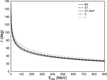
Figure 4: The $S$-wave phase shifts for $\phi\phi$ scattering with one $\sigma$-exchange as the potential using the BS, ET, ET-NAP, C, and I equations.

To emulate the $NN$ system in the $\phi^{2}\sigma$ model with $\sigma$ exchange as the potential, we have chosen the mass of the $\phi$ ($N)$ to be 1 GeV, while the $\sigma$ ($\pi$) has a mass of $0.15$ GeV. For $S$-wave scattering we have adjusted the coupling constant so that the $\phi\phi$ system has a bound state with a binding energy $2.2$ MeV corresponding to the deuteron. In Fig. 4 we present the phase shifts resulting from the solution of the BS equation as well as the equal-time, Cohen, and the instantaneous 3-D equations. Also included are the phase shifts resulting from the equal-time equation after excluding the negative energy component of the propagator (ET-NAP), i.e., we have excluded the left hand cut and hence violated charge conjugation symmetry. This situation corresponds to time-ordered perturbation theory Lahiff and Afnan (1997), which has been used frequently in models of $NN$ scattering (see, e.g., Ref. Machleidt (1989)) and $\pi N$ scattering (see, e.g., Ref. Durso et al. (1994)). From the results in Fig. 4 we find, as expected, no great variation as one excludes higher unitarity cuts. On the other hand, the differences are consistent with the unitarity analysis of the last section in that the best approximation is the ET equation, followed by C, ET-NAP, and finally I. It is interesting to note that the inclusion of the three-body unitarity cut in the ET-NAP equation is more important than satisfying charge conjugation which is included in the I equation.

A better test of the role of higher unitarity cuts is to examine the inelasticity for the different approximations to the BS equation, the results of which are shown in Fig. 5. In this case results for the I equation have not been included since the inelasticity is always unity, as this equations include the two-body unitarity cuts only. The agreement between the BS and ET equations is a result of the fact that both equations have the same three-body unitarity cuts. The Cohen equation does not have a three-body unitarity cut, and as a result, the inelasticity for this equation is less than one only for energies above the four-body unitarity threshold. At this stage the results for the BS and ET equations start to deviate as the latter does not include the four-body thresholds. Although we can observe differences between the equations in the inelasticity, in all cases the inelasticity is very small for this problem.

From the above analysis we may conclude that for energies close to the $\sigma$ production threshold, the ET equation handles the inelasticity much better than any of the other 3-D equations as it includes the same three-body unitarity cuts that the BS equation has.

We now turn to the $\pi N$ system, and consider a model in which the potential includes $N$ and $\Delta$ $s$- and $u$-channel pole diagrams as well as $\sigma$ and $\rho$ $t$-channel pole diagrams. To solve the BS equation or one of the 3-D equations for the $\pi N$ system we need to introduce some form of regularization. This has been achieved by introducing two types Lahiff and Afnan (1999) of form factors for each of the vertices in the diagrams that constitute the potential.

• Type I: Since the vertices in the potentials have three legs, we can write a form factor for each vertex as the product of three functions of the four-momenta of the three legs, i.e.,

  $$f_{\alpha\beta\gamma}(p_{\alpha}^{2},p_{\beta}^{2},p_{\gamma}^{2})=f_{\alpha}(p_{\alpha}^{2})\,f_{\beta}(p_{\beta}^{2})\,f_{\gamma}(p_{\gamma}^{2})\ ,$$ (40)

  where $\alpha$, $\beta$, and $\gamma$ refer to the three legs of the vertex. The function $f_{\alpha}(p_{\alpha}^{2})$ is taken to be

  $$f_{\alpha}(p_{\alpha}^{2})=\left(\frac{\Lambda_{\alpha}^{2}-m_{\alpha}^{2}}{\Lambda_{\alpha}^{2}-p_{\alpha}^{2}}\right)^{n_{\alpha}}\ ,$$ (41)

  with $n_{\alpha}=1$. Here $m_{\alpha}$ is the mass of the particle, while $\Lambda_{\alpha}$ is the cutoff mass that is a parameter of the potential. Since such form factors have poles, they can generate unphysical thresholds. To minimize the effect of these unphysical thresholds, we have constrained the cutoff masses $\Lambda_{\alpha}$ to ensure that these thresholds are at much higher energies than any of the physical thresholds we are examining.

• Type II: To reduce the number of cutoff masses, and at the same time employ a form factor that is more commonly used, we have taken the form factor to depend on the four-momentum of the pion only, i.e.,

  $$f_{\alpha\beta\gamma}(p_{\alpha}^{2},p_{\beta}^{2},p_{\gamma}^{2})=f_{\pi}(p_{\pi}^{2})\ .$$ (42)

  Here we present results for $n=4$ only.

The parameters of the BS potential and form factors have been adjusted to fit the $\pi N$ data up to a laboratory energy of 360 MeV Lahiff and Afnan (1999). We use the BS parameters in the different 3-D equations, i.e., we do not refit the parameters using each of the scattering equations. This is so that the effects of the different 3-D reductions can be easily compared to the BS equation.

In Fig. 6 we present the $S_{11}$ and $S_{31}$ phase shifts for the two types of form factors and the different 3-D approximations to the BS equation. Also included are the results of the VPI SM95 Arndt et al. (1995) partial wave analysis. In this case it is not clear as to which 3-D equation gives the best approximation to the BS equation. This is partly due to the fact that the final amplitude is not dominated by any single one of the diagrams that contribute to the potential. In both the $S_{11}$ and $S_{31}$ partial waves there are large cancellations between the various diagrams that contribute to the potential.

To see a more pronounced difference between the different equations, we turn next to the $P_{11}$ partial wave. In this case the amplitude is dominated by the $s$-channel pole diagram, which is repulsive, as well as the $u$-channel $\Delta$ pole, which is attractive. In Fig. 7 we present our results for the two different types of form factor. Here it is clear that ET equation gives the best approximation to the BS equation, but the variation between the different equations is not significant provided we restrict our regularization to type II form factors that depend on the four-momentum of the pion only. For the type I form factor the BbS equation gives very poor results. At this stage we note that the BbS equation gives additional attraction when compared to the BS equation.

We finally turn to the $P_{33}$ partial wave which is dominated by just one term in the potential: the $s$-channel $\Delta$ pole diagram. Here (see Fig. 8) there is a dramatic change as one goes from the BS equation to the ET equation to the Cohen equation, and finally to the equations with just the two-body unitarity thresholds. The trend in the phase shifts suggests that the additional attraction generated by neglecting the higher unitarity cuts is slowly converting the resonance pole to a bound state pole. If it is the higher unitarity cuts that are the source of this difference, then these cuts would be even more important for higher-energy resonances in the $\pi N$ system. This is a question that would require further investigation.

For the case of type I form factors, tables of the numerical results are presented in Appendix C.

We do not present results for the inelasticities in the $\pi N$ system, because the inelasticity generated by the BS equation and the different 3-D equations is negligible for the energy range considered here.

V Conclusion

In the preceding analysis we have demonstrated that the Bethe-Salpeter equation in the ladder approximation has in addition to the two-body unitarity cut, a selected set of $n$-body unitarity cuts. In reducing the dimensionality of the BS equation from four to three it is possible to preserve some of the three- or four-body unitarity cuts and in this way preserve some of the features of the original equation. This could be important at energies close to the three-body threshold, as is the case for the $\pi N$ system in the region of the lowest resonances. From the numerical results presented for the two models considered, we may conclude that the preservation of these higher unitarity cuts do in general result in an equation that is a better approximation to the BS equation. In particular, for the $\Delta$ resonance, the inclusion of these higher thresholds are of considerable importance.

It is always possible to readjust the parameters of the potential within the framework of any one of these equations to fit the experimental data. This procedure will result in the coupling constants in the Lagrangian being different from those resulting from the use of the BS equation. As long as those coupling constants have little physical meaning one may justify using any scattering equation that preserves two-body unitarity. However, if we would like some consistency, e.g. between the $\pi N$ and $NN$ systems, then it may be important to reduce the approximations in the starting equation. More significant is the possibility of missing some physical mechanisms such as the contribution of three-body thresholds to resonances just above the pion production threshold.

Although three-body unitarity is not completely included in the ladder approximation to the BS equation, one could add further contributions to three-body unitarity by dressing the nucleon in the $\pi N$ propagator. That will play an important role if the BS equation is to include coupling to other channels such as the $\pi\Delta$ channel.

Appendix A Thresholds in the Equal-Time Equation

To illustrate the thresholds generated in the equal-time formalism Klein (1953); Phillips and Wallace (1996); Lahiff and Afnan (1997), we consider the singularities of

$$\langle G\,V\,G\rangle = \int\limits_{-\infty}^{+\infty}\,dq_{0}\ \frac{1}{\left(\frac{\sqrt{s}}{2}-q_{0}\right)^{2}-E_{q}^{2}+i\epsilon}\,\frac{1}{\left(\frac{\sqrt{s}}{2}+q_{0}\right)^{2}-E_{q}^{2}+i\epsilon}$$

$$\times\int\limits_{-\infty}^{+\infty}dq^{\prime}_{0}\ \frac{1}{\left(q_{0}-q^{\prime}_{0}\right)^{2}-\omega^{2}_{q-q^{\prime}}+i\epsilon}\,\frac{1}{\left(\frac{\sqrt{s}}{2}-q^{\prime}_{0}\right)^{2}-E_{q^{\prime}}^{2}+i\epsilon}\,\frac{1}{\left(\frac{\sqrt{s}}{2}+q^{\prime}_{0}\right)^{2}-E_{q^{\prime}}^{2}+i\epsilon}\ .$$

The singularity structure of $\langle G\,V\,G\rangle$ is determined by the pinching of the $q_{0}$ and $q^{\prime}_{0}$ contours by the poles in the integrand. For the $q^{\prime}_{0}$ integration, we have poles from both the propagators and the potential. As we have not partial wave expanded the potential we have at this stage only poles. However, upon partial wave expansion these poles will generate logarithmic branch points which we will enumerate.

In the $q^{\prime}_{0}$ plane we have the four propagator poles:

$$1)\quad q^{\prime}_{0} = -\frac{1}{2}\sqrt{s}-E_{q^{\prime}}+i\epsilon\ ;\quad\quad 2)\quad q^{\prime}_{0}=\frac{1}{2}\sqrt{s}-E_{q^{\prime}}+i\epsilon\ ;$$

$$3)\quad q^{\prime}_{0} = -\frac{1}{2}\sqrt{s}+E_{q^{\prime}}-i\epsilon\ ;\quad\quad 4)\quad q^{\prime}_{0}=\frac{1}{2}\sqrt{s}+E_{q^{\prime}}-i\epsilon\ .$$ (44)

On the other hand the potential branch points in the $q^{\prime}_{0}$-plane are at

$$5)\quad q^{\prime}_{0} = q_{0}-\omega_{q+q^{\prime}}+i\epsilon\ ;\quad\quad 6)\quad q^{\prime}_{0}=q_{0}-\omega_{q-q^{\prime}}+i\epsilon\ ;$$

$$7)\quad q^{\prime}_{0} = q_{0}+\omega_{q+q^{\prime}}-i\epsilon\ ;\quad\quad 8)\quad q^{\prime}_{0}=q_{0}+\omega_{q-q^{\prime}}-i\epsilon\ .$$ (45)

For $\sqrt{s}>0$, the pinching of the $q^{\prime}_{0}$ contour of integration is between the following singularities:

• Between two of the poles of the propagator, and in particular for $\sqrt{s}>0$, poles $2)$ and $3)$ pinch the contour provided

  $$\sqrt{s}=2E_{q^{\prime}}-2i\epsilon\ .$$ (46)

  In a similar manner for $\sqrt{s}<0$, poles $1)$ and $4)$ pinch the contour to generate a branch cut at $\sqrt{s}=-2E_{q}+2i\epsilon$. These will generate thresholds at $\sqrt{s}=\pm 2m$.

• Between one of the poles of the propagator and a branch point of the potential. In particular singularities 3) and 6) pinch the contour if

  $$9)\quad q_{0}=-\frac{1}{2}\sqrt{s}+E_{q^{\prime}}+\omega_{q-q^{\prime}}-2i\epsilon\ .$$ (47)

  This branch point is going to be involved in the pinching of the $q_{0}$ integration contour, and to that extent will not at this stage generate a threshold in the final amplitude. Although the $q_{0}$ integration includes the on-shell point $q_{0}=0$, we do not expect this singularity to generate a threshold in the amplitude, since we can deform the $q_{0}$ contour of integration to avoid the point $q_{0}=0$.

  Similarly the propagator pole $2)$ and the branch point $8)$ pinch the $q^{\prime}_{0}$ contour provided

  $$10)\quad q_{0}=\frac{1}{2}\sqrt{s}-E_{q^{\prime}}-\omega_{q-q^{\prime}}+2i\epsilon\ .$$ (48)

A similar set of branch points are generated for $\sqrt{s}<0$. In this case the propagator poles $1)$ and $4)$ (see Fig. 1) pinch the $q_{0}^{\prime}$ integration contour to produce a branch point at $\sqrt{s}=-2m$. On the other hand the pinching of the $q^{\prime}_{0}$ by the propagator pole $1)$ and the potential branch point $8)$ generates a branch point in the $q_{0}$ plane at the point $q_{0}=-\frac{1}{2}\sqrt{s}-E_{q^{\prime}}-\omega_{q-q^{\prime}}+2i\epsilon$. This is a reflection of the branch point in Eq. (48) in the $\sqrt{s}$-plane. In a similar manner, we get a reflection in the $\sqrt{s}$-plane of the branch point in Eq. (47) when the pole $4)$ and the branch point $6)$ pinch the $q^{\prime}_{0}$ contour. In this way the ET formulation maintains analyticity in $s$.

We now turn to the $q_{0}$ integration. In this case the singularities of the integrand arise from the propagator poles and those generated by the $q^{\prime}_{0}$ integration. The propagator poles are at:

$$11)\quad q_{0} = -\frac{1}{2}\sqrt{s}-E_{q}+i\epsilon\ ;\quad 12)\quad q_{0}=\frac{1}{2}\sqrt{s}-E_{q}+i\epsilon\ ;$$

$$13)\quad q_{0} = -\frac{1}{2}\sqrt{s}+E_{q}-i\epsilon\ ;\quad 14)\quad q_{0}=\frac{1}{2}\sqrt{s}+E_{q}-i\epsilon\ .$$ (49)

In this case the $q_{0}$ contour can be pinched by the following singularities:

• For $\sqrt{s}>0$, propagator poles $12)$ and $13)$ pinch the $q_{0}$ contour to give the branch cut

  $$\sqrt{s}=2E_{q}-2i\epsilon\ ,$$ (50)

  while for $\sqrt{s}<0$ the poles $11)$ and $14)$ pinch the contour to generate a branch cut at $\sqrt{s}=-2E_{q}+2i\epsilon$. These will generate the two-body threshold $\sqrt{s}=\pm 2m$.

• The propagator pole 12) and the branch cut generated by the $q^{\prime}_{0}$ integration 9) can pinch the $q_{0}$ contour. The condition for this pinch is

  $$\sqrt{s}=E_{q}+E_{q}^{\prime}+\omega_{q-q^{\prime}}-3i\epsilon\ .$$ (51)

  Since this is in the kernel of the three-dimensional integral equation, the actual pinch takes place at $q^{\prime}=0$. As a result this will generate a branch point at $\sqrt{s}=2m+\mu$.

  In a similar manner the propagator pole 13) and the branch cut generated by the $q^{\prime}_{0}$ integration 10) can pinch the $q_{0}$ contour. In this case the pinch takes place if

  $$\sqrt{s}=E_{q}+E_{q}^{\prime}+\omega_{q-q^{\prime}}-3i\epsilon\ ,$$ (52)

  which is identical to that in Eq. (51), and will generate the three-body threshold at $\sqrt{s}=2m+\mu$. A similar set of pinchings of the $q_{0}$ contour takes place between the poles of the propagators and the branch points generated by the $q^{\prime}_{0}$ integration for $\sqrt{s}<0$ to generate the three-body threshold at $\sqrt{s}=-(2m+\mu)$.

In this way we have established that the equal time equation generates an amplitude that has two- and three-body thresholds and is analytic in $s$. Unfortunately, not all possible three-body thresholds are included, and therefore the resultant equation does not satisfy three-body unitarity.

Appendix B 3-D equations for $\pi N$ Scattering

For completeness, in this appendix we give explicit forms for the different 3-D equations discussed in the present work. Since some 3-D equations violate Lorentz invariance, for example the BbS equation, the solutions of such equations depend on the choice of the relative four-momentum. Here we use the commonly-used choice

$$\alpha_{N}(s)=\frac{s+m_{N}^{2}-\mu_{\pi}^{2}}{2s},\hskip 28.45274pt\alpha_{\pi}(s)=\frac{s+\mu_{\pi}^{2}-m_{N}^{2}}{2s}.$$ (53)

In this section we make use of $\pi N\rightarrow\pi N$ amplitudes sandwiched between Dirac spinors. We use the following notation for the amplitudes:

$$T^{\bar{u}u}(q^{\prime},q;s) = \bar{u}(\textbf{q}^{\prime})T(q^{\prime},q;s)u(\textbf{q}),$$ (54a)

$$T^{\bar{v}u}(q^{\prime},q;s) = \bar{v}(-\textbf{q}^{\prime})T(q^{\prime},q;s)u(\textbf{q}),$$ (54b)

and similarly for the potentials. With this notation, the BS equation has the form of two coupled equations for $T^{\bar{u}u}$ and $T^{\bar{v}u}$ Lahiff and Afnan (1999):

$$T^{\bar{w}u}(q^{\prime},q;P)=V^{\bar{w}u}(q^{\prime},q;P)-{i\over(2\pi)^{4}}\sum_{w^{\prime\prime}=u,v}\int d^{4}q^{\prime\prime}\,V^{\bar{w}w^{\prime\prime}}(q^{\prime},q^{\prime\prime};P)G^{\bar{w}^{\prime\prime}w^{\prime\prime}}_{\pi N}(q^{\prime\prime};P)T^{\bar{w}^{\prime\prime}u}(q^{\prime\prime},q;P),$$ (55)

with $w=u\mbox{, }v$. The $\pi N$ propagators $G^{\bar{w}^{\prime\prime}w^{\prime\prime}}_{\pi N}$ are defined in Eq. (27).

Firstly we consider the Cohen equation, which has the form (before partial wave expansion)

$$T^{\bar{w}u}(\textbf{q}^{\prime},\textbf{q};s)=V^{\bar{w}u}(0,\textbf{q}^{\prime};0,\textbf{q};s)-{i\over(2\pi)^{4}}\sum_{w^{\prime\prime}=u,v}\int d\textbf{q}^{\prime\prime}\,\tilde{K}^{\bar{w}w^{\prime\prime}}(\textbf{q}^{\prime},\textbf{q}^{\prime\prime};s)T^{\bar{w}^{\prime\prime}u}(\textbf{q}^{\prime\prime},\textbf{q};s),$$ (56)

with the kernel given by

$$\tilde{K}^{\bar{w}^{\prime}w}(\textbf{q}^{\prime},\textbf{q};s)=\int_{-\infty}^{\infty}dq_{0}V^{\bar{w}^{\prime}w}(0,\textbf{q}^{\prime};q_{0},\textbf{q};s)G_{\pi N}^{\bar{w}w}(q_{0},q;s).$$ (57)

The relative energy integration can be carried out by making use of the Wick rotation Wick (1954).

The remaining 3-D equations for $\pi N$ scattering have the form

$$T^{\bar{w}u}(\textbf{q}^{\prime},\textbf{q};s)=K^{\bar{w}u}(\textbf{q}^{\prime},\textbf{q};s)-{i\over(2\pi)^{4}}\sum_{w^{\prime\prime}=u,v}\int d\textbf{q}^{\prime\prime}\,K^{\bar{w}w^{\prime\prime}}(\textbf{q}^{\prime},\textbf{q}^{\prime\prime};s)g^{\bar{w}^{\prime\prime}w^{\prime\prime}}_{\pi N}(q^{\prime\prime};s)T^{\bar{w}^{\prime\prime}u}(\textbf{q}^{\prime\prime},\textbf{q};s).$$ (58)

The two-body $\pi N$ propagators are denoted as $g^{\bar{u}u}_{\pi N}$ and $g^{\bar{v}v}_{\pi N}$, which contain the positive and negative energy components of the nucleon propagator, respectively. The 3-D potentials are denoted as $K^{\bar{w}^{\prime}w}$.

To our knowledge the ET equation for $\pi N$ scattering has not been previously discussed in the literature. The two-body $\pi N$ propagator appearing in the ET equation is obtained from the propagator in the BS equation by integrating out the relative energy, i.e.,

$$g_{\pi N}(\textbf{q};s) = \int_{-\infty}^{\infty}dq_{0}G_{\pi N}(q_{0},\textbf{q};s)$$ (59)

$$= 2\pi i{m_{N}\over 2E_{q}\omega_{q}}\left({\Lambda^{+}(\textbf{q})\over\sqrt{s}-E_{q}-\omega_{q}+i\epsilon}+{\Lambda^{-}(-\textbf{q})\over\sqrt{s}+E_{q}+\omega_{q}-i\epsilon}\right)$$

$$\equiv g_{\pi N}^{\bar{u}u}(q;s)\Lambda^{+}(\textbf{q})+g_{\pi N}^{\bar{v}v}(q;s)\Lambda^{-}(-\textbf{q}).$$

For the calculation of the ET potential, we will also need the inverse of $g_{\pi N}$, which is given by

$$g_{\pi N}(\textbf{q};s)^{-1}={1\over 2\pi i}{2m_{N}\omega_{q}\over E_{q}}\Biggl{(}[\sqrt{s}-E_{q}-\omega_{q}]\Lambda^{+}(-\textbf{q})+[\sqrt{s}+E_{q}+\omega_{q}]\Lambda^{-}(\textbf{q})\Biggr{)}\ .$$ (60)

The potential for the ET equation is then

$$K(\textbf{q}^{\prime},\textbf{q};s) = g_{\pi N}(\textbf{q}^{\prime};s)^{-1}\int_{-\infty}^{\infty}dq^{\prime}_{0}\int_{-\infty}^{\infty}dq_{0}G_{\pi N}(q^{\prime}_{0},\textbf{q}^{\prime};s)V(q^{\prime}_{0},\textbf{q}^{\prime};q_{0},\textbf{q};s)G_{\pi N}(q_{0},\textbf{q};s)$$ (61)

$$\times g_{\pi N}(\textbf{q};s)^{-1}.$$

Multiplying Eq. (61) from the left and right by Dirac spinors, and making use of the orthonormality of Dirac spinors, we find

$$K^{\bar{w}^{\prime}w}(\textbf{q}^{\prime},\textbf{q};s) = -{1\over(2\pi)^{2}}{2E_{q^{\prime}}\omega_{q^{\prime}}\over m_{N}}{2E_{q}\omega_{q}\over m_{N}}\left(\sqrt{s}-\xi^{\prime}E_{q^{\prime}}-\xi^{\prime}\omega_{q^{\prime}}\right)\left(\sqrt{s}-\xi E_{q}-\xi\omega_{q}\right)$$ (62)

$$\times\int_{-\infty}^{\infty}dq^{\prime}_{0}\int_{-\infty}^{\infty}dq_{0}G_{\pi N}^{\bar{w}^{\prime}w^{\prime}}(q^{\prime}_{0},q^{\prime};s)V^{\bar{w}^{\prime}w}(q^{\prime}_{0},\textbf{q}^{\prime};q_{0},\textbf{q};s)G_{\pi N}^{\bar{w}w}(q_{0},q;s).$$

Here $\xi^{\prime}=+1$ ($-1$) for $w^{\prime}=u$ ($v$), and $\xi=+1$ ($-1$) for $w=u$ ($v$). Again, the relative energy integrations above can be performed numerically by making use of the Wick rotation Wick (1954), which can be applied in the same way as it is used in solving the BS equation Lahiff and Afnan (1999).

For the instantaneous equation, the $g^{\bar{w}w}_{\pi N}$ are obtained by integrating out the relative energy of the $\pi N$ propagator appearing in the BS equation, and so we have

$$g^{\bar{u}u}_{\pi N}(q;s) = {\pi im_{N}\over E_{q}\omega_{q}[\sqrt{s}-E_{q}-\omega_{q}+i\epsilon]},$$ (63a)

$$g^{\bar{v}v}_{\pi N}(q;s) = {\pi im_{N}\over E_{q}\omega_{q}[\sqrt{s}+E_{q}+\omega_{q}-i\epsilon]}.$$ (63b)

It is clear that the ET and I equations make use of the same $\pi N$ propagator.

The BbS equation is obtained by replacing $G_{\pi N}$ in the BS equation with the following two-body propagator

$$G^{\rm BbS}_{\pi N}(q;P)=2\pi i\int_{s_{th}}^{\infty}\frac{ds^{\prime}}{s^{\prime}-s-i\epsilon}[\alpha_{N}P/\,^{\prime}+q/+m_{N}]\delta^{(+)}[(\alpha_{N}P^{\prime}+q)^{2}-m_{N}^{2}]\delta^{(+)}[(\alpha_{\pi}P^{\prime}-q)^{2}-\mu_{\pi}^{2}],$$ (64)

where $s_{th}=(m_{N}+\mu_{\pi})^{2}$, and $P^{\prime}=(\sqrt{s^{\prime}}/\sqrt{s})P$. This results in the BS equation being reduced to a 3-D equation of the form of Eq. (58), with the $\pi N$ propagators given by

$$g^{\bar{u}u}_{\pi N}(q;s) = {2\pi im_{N}\over E_{q}\omega_{q}[s-(E_{q}+\omega_{q})^{2}+i\epsilon]},$$ (65a)

$$g^{\bar{v}v}_{\pi N}(q;s) = 0.$$ (65b)

Notice that the coupling to negative energy states is neglected, but $g^{\bar{u}u}_{\pi N}$ has poles at both $\sqrt{s}=E_{q}+\omega_{q}$ and $\sqrt{s}=-E_{q}-\omega_{q}$.

In the I equation the potential is assumed to be static, while for the BbS equation the relative energy is fixed at its on-shell value. Therefore the potentials for these two equations are given by

$$K^{\bar{w}^{\prime}w}(\textbf{q}^{\prime},\textbf{q};s)=V^{\bar{w}^{\prime}w}(0,\textbf{q}^{\prime};0,\textbf{q};s).$$ (66)

The differences between the I and BbS equations lie in the form used for the $\pi N$ propagator.

Appendix C Tabulated Results

Tables 1 to 4 show the numerical values of the $\pi N$ phase shifts when type I form factors are used.

$E_{\mbox{\scriptsize lab}}$	BS	ET	C	I	BbS
$50$	$6.78$	$6.30$	$6.34$	$7.34$	$9.33$
$100$	$9.17$	$7.84$	$7.96$	$9.18$	$12.9$
$150$	$10.2$	$8.05$	$8.12$	$8.76$	$13.0$
$200$	$10.3$	$7.42$	$7.35$	$7.39$	$12.3$
$250$	$9.76$	$6.21$	$5.92$	$5.40$	$11.0$
$300$	$8.72$	$4.62$	$4.06$	$2.95$	$9.13$
$350$	$7.18$	$2.74$	$1.90$	$0.191$	$6.85$

Table 1: The $S_{11}$ phase shifts using the type I form factors as calculated by the BS equation and the different 3-D quasipotential equations.

$E_{\mbox{\scriptsize lab}}$	BS	ET	C	I	BbS
$50$	$-5.46$	$-3.73$	$-5.93$	$-5.52$	$-5.21$
$100$	$-8.73$	$-5.96$	$-9.24$	$-9.34$	$-8.45$
$150$	$-11.9$	$-8.02$	$-12.3$	$-13.0$	$-11.4$
$200$	$-15.0$	$-9.96$	$-15.1$	$-16.5$	$-14.4$
$250$	$-18.2$	$-11.8$	$-18.0$	$-20.2$	$-17.4$
$300$	$-21.4$	$-13.6$	$-20.7$	$-24.3$	$-20.5$
$350$	$-24.9$	$-15.3$	$-23.5$	$-28.7$	$-23.7$

Table 2: The $S_{31}$ phase shifts using the type I form factors as calculated by the BS equation and the different 3-D quasipotential equations.

$E_{\mbox{\scriptsize lab}}$	BS	ET	C	I	BbS
$50$	$-1.09$	$-1.21$	$-1.50$	$-1.07$	$0.266$
$100$	$-1.53$	$-1.40$	$-2.46$	$-2.34$	$1.65$
$150$	$-0.50$	$0.159$	$-1.36$	$-1.52$	$4.60$
$200$	$2.45$	$3.793$	$2.03$	$1.62$	$10.9$
$250$	$7.75$	$9.78$	$8.26$	$7.95$	$23.6$
$300$	$15.7$	$18.1$	$17.7$	$18.4$	$45.2$
$350$	$25.9$	$28.10$	$20.7$	$32.7$	$70.9$

Table 3: The $P_{11}$ phase shifts using the type I form factors as calculated by the BS equation and the different 3-D quasipotential equations.

$E_{\mbox{\scriptsize lab}}$	BS	ET	C	I	BbS
$50$	$4.85$	$4.61$	$8.23$	$174.0$	$180.0$
$100$	$18.7$	$16.7$	$45.4$	$171.0$	$181.0$
$150$	$51.6$	$42.2$	$111.0$	$169.0$	$182.0$
$200$	$96.0$	$80.5$	$133.0$	$167.0$	$183.0$
$250$	$120.0$	$108.0$	$141.0$	$165.0$	$183.0$
$300$	$131.0$	$121.0$	$144.0$	$164.0$	$183.0$
$350$	$138.0$	$131.0$	$147.0$	$163.0$	$183.0$

Table 4: The $P_{33}$ phase shifts using the type I form factors as calculated by the BS equation and the different 3-D quasipotential equations.

Figure 2: The branch points of the potential in the $q^{\prime\prime}_{0}$-plane.

Figure 3: The branch points of the amplitude resulting from the pinching of the integration contour by the propagator poles and potential branch points in the $q^{\prime\prime}_{0}$-plane. The arrows indicate the direction in which the branch points move with increasing $s$.

Figure 5: The inelasticity $\eta$ for the BS, ET, ET-NAP, and C equations.

Figure 6: The $S_{11}$ and $S_{31}$ phase shifts for the type II (a) and type I (b) form factors. The data points are from Arndt et al. (1995).

Figure 7: The $P_{11}$ phase shifts for the type II (a) and type I (b) form factors. The data points are from Arndt et al. (1995).

Figure 8: The $P_{33}$ phase shifts for the type II (a) and type I (b) form factors. The data points are from Arndt et al. (1995).

References

- Salpeter and Bethe (1951) E. E. Salpeter and H. A. Bethe, Phys. Rev. 84, 1232 (1951).
- Klein and Lee (1974) A. Klein and T.-S. H. Lee, Phys. Rev. D 10, 4308 (1974).
- Gross (1982) F. Gross, Phys. Rev. C 26, 2203 (1982).
- Mandelzweig and Wallace (1987) V. B. Mandelzweig and S. J. Wallace, Phys. Lett. B197, 469 (1987).
- Wallace and Mandelzweig (1989) S. J. Wallace and V. B. Mandelzweig, Nucl. Phys. A503, 673 (1989).
- Phillips and Wallace (1996) D. R. Phillips and S. J. Wallace, Phys. Rev. C 54, 507 (1996).
- Gross and Surya (1993) F. Gross and Y. Surya, Phys. Rev. C 47, 703 (1993).
- Pascalutsa (1995) V. Pascalutsa, Ph.D. thesis, University of Utrecht (1995).
- Pascalutsa and Tjon (1999) V. Pascalutsa and J. A. Tjon, Phys. Rev. C 60, 034005 (1999).
- Bakamjian and Thomas (1953) B. Bakamjian and L. Thomas, Phys. Rev. 92, 1300 (1953).
- Keister and Polyzou (1991) B. Keister and W. N. Polyzou, Adv. Nucl. Phys. 20, 225 (1991).
- Fuda (1995) M. Fuda, Phys. Rec. C 52, 2875 (1995).
- Elmessiri and Fuda (1998) Y. Elmessiri and M. Fuda, Phys. Rec. C 57, 2149 (1998).
- Elmessiri and Fuda (1999) Y. Elmessiri and M. Fuda, Phys. Rec. C 60, 044001 (1999).
- Ohkuba (1954) S. Ohkuba, Prog. Theor. Phys. 12, 603 (1954).
- Lahiff and Afnan (1999) A. D. Lahiff and I. R. Afnan, Phys. Rev. C 60, 024608 (1999).
- Klein (1953) A. Klein, Phys. Rev. 90, 1101 (1953).
- Lahiff and Afnan (1997) A. D. Lahiff and I. R. Afnan, Phys. Rev. C 56, 2387 (1997).
- Cohen (1970) H. Cohen, Phys. Rev. D 2, 1738 (1970).
- Salpeter (1952) E. E. Salpeter, Phys. Rev. 87, 328 (1952).
- Pascalutsa and Tjon (2000) V. Pascalutsa and J. A. Tjon, Phys. Rev. C 61, 054003 (2000).
- Blankenbecler and Sugar (1966) R. Blankenbecler and R. Sugar, Phys. Rev. 142, 1051 (1966).
- Pagnamenta and Taylor (1966) A. Pagnamenta and J. G. Taylor, Phys. Rev. Lett. 17, 218 (1966).
- Pearce and Jennings (1991) B. C. Pearce and B. K. Jennings, Nucl. Phys. A528, 655 (1991).
- Wick (1954) G. C. Wick, Phys. Rev. 96, 1124 (1954).
- Eden (1952) R. J. Eden, Proc. Roy. Soc. A 210, 388 (1952).
- Eden (1962) R. J. Eden, Lectures in Theoretical Physics (W. A. Benjamin, New York, 1962).
- Pascalutsa and Tjon (1998) V. Pascalutsa and J. A. Tjon, Phys. Lett. B435, 245 (1998).
- Phillips and Afnan (1996) D. R. Phillips and I. R. Afnan, Phys. Rev. C 54, 1542 (1996).
- Machleidt (1989) R. Machleidt, Adv. Nucl. Phys. 19, 189 (1989).
- Durso et al. (1994) J. W. Durso, K. Holinde, and J. Speth, Phys. Rev. C 49, 2671 (1994).
- Arndt et al. (1995) R. A. Arndt, I. I. Strakovsky, R. L. Workman, and M. M. Pavan, Phys. Rev. C 52, 2120 (1995).