Effective Field Theory for Halo Nuclei: Shallow $p$-Wave States

Abstract

Halo nuclei are a promising new arena for studies based on effective field theory (EFT). We develop an EFT for shallow $p$-wave states and discuss the application to elastic $n\alpha$ scattering. In contrast to the $s$-wave case, both the scattering length and effective range enter at leading order. We also discuss the prospects of using EFT in the description of other halos, such as the three-body halo nucleus ⁶He.

I Introduction

Nuclear halo states have been found in a number of light nuclei close to the nucleon drip lines. They are characterized by a very low separation energy of the valence nucleon (or cluster of nucleons). As a consequence, the nuclear radius is very large compared to the size of the tightly bound core. The large size of halo nuclei leads to threshold phenomena with important general consequences for low-energy reaction rates in nuclear astrophysics. One example is the reaction $p+\mbox{${}^{7}$Be}\to\mbox{${}^{8}$B}+\gamma$ which is important for solar neutrino production. The nucleus ⁸B is believed to be a two-body proton halo, consisting of a ⁷Be core and a proton BCS96 . Somewhat more complicated are three-body halos consisting of a core and two slightly bound nucleons. Particularly interesting are Borromean three-body halos, where no two-body subsystem is bound. Typical examples are ⁶He and ¹¹Li, which consist of a ⁴He and ⁹Li core, respectively, and two neutrons. For reviews of halo nuclei, see Ref. ZDF93 . The physics of halo nuclei is an important part of the physics program at RIA RIA00 . A thorough discussion of reactions with rare isotopes can be found in Ref. BHM02 .

The physics of halo nuclei is a promising new arena for Effective Field Theory (EFT). EFTs provide a powerful framework to explore separation of scales in physical systems in order to perform systematic, model-independent calculations EFT . If, for example, the relative momentum $k$ of two particles is much smaller than the inverse range of their interaction $1/R$, observables can be expanded in powers of $kR$. All short-distance effects are systematically absorbed into a few low-energy constants using renormalization. The EFT approach allows for systematically improvable calculations of low-energy processes with well-defined error estimates. The long-distance physics is included explicitly, while the corrections from short-distance physics are calculated in an expansion in the ratio of these two scales. The inherent separation of length scales in halo nuclei makes them an ideal playing ground for EFT.

In recent years, there has been much interest in applying EFT methods to nuclear systems Birareview ; NN99 . Up to now, nuclear EFT has mainly been applied to two-, three-, and four-nucleon systems starting from a fundamental nucleon-nucleon interaction. The original motivation was to understand the gross features of nuclear systems from a QCD perspective by deriving the nuclear potential and currents relevant for momenta comparable to the pion mass ($p\sim m_{\pi}$) Weinberg . More recently, it has been realized that it is possible to carry out very precise calculations for fundamental physics processes at lower energies. For very low momenta ($p\hskip 1.99997pt\raisebox{2.15277pt}{$<$}\raisebox{-3.00003pt}{$\sim$}\hskip 1.99997ptm_{\pi}$), even pion exchange can be considered “short-distance” physics. In this case, one can use an effective Lagrangian including only contact interactions. The large $s$-wave scattering lengths require that the leading two-body contact interaction be treated nonperturbatively vKo99 ; KSW98 . In the two-nucleon system, this program has been very successful (see, e.g., Refs. CRS99 ; Birareview and references therein).

Using EFT, one can relate low-energy measurements in one reaction to observables in a similar (but unmeasured) reaction in a controlled expansion with reliable error estimates. This is in contrast to standard potential model calculations where errors can only be estimated by comparing different potentials. An example of a precise calculation in the “pionless” EFT is the reaction $n+p\to d+\gamma$ ChS99 , which is relevant to big-bang nucleosynthesis (BBN). As for many other reactions of astrophysical interest, the uncertainty in the cross section is difficult to determine due to the lack of data at low energies and the lack of information about theoretical estimates. In the energy of relevance to BBN, both $E1$ and $M1$ capture are important. They have been calculated to fifth and third order, respectively, where two new counterterms appear. Using the measured cold-capture rate and data for the deuteron photodisintegration reaction to fix the counterterms, the $n+p\to d+\gamma$ cross section was computed to 1% for center-of-mass energies $E\hskip 1.99997pt\raisebox{2.15277pt}{$<$}\raisebox{-3.00003pt}{$\sim$}\hskip 1.99997pt1$ MeV.

Much of the strength of EFT lies in the fact that it can be applied without off-shell ambiguities to systems with more nucleons. The crucial issue of the relative size of three-body forces has been investigated in the three-body system BHK99 . Nucleon-deuteron scattering in all channels except the $s_{1/2}$ wave can be calculated to high orders using two-nucleon input only, with results in striking agreement with data and potential-model calculations BeK98 . For example, to third order, the $s_{3/2}$ scattering length is found to be $a_{3/2}^{(EFT)}=6.33\pm 0.10$ fm, to be compared to the measured $a_{3/2}^{(expt)}=6.35\pm 0.02$ fm. In contrast, in the $s_{1/2}$-wave channel, the non-perturbative running of the renormalization group requires a momentum-independent three-body force in leading order BHK00 . Once the new parameter is fitted to (say) the scattering length, the energy dependence is predicted. The triton binding energy, for example, is found to be $B_{3}^{(EFT)}=8.0$ MeV in leading order, already pretty close to the experimental $B_{3}^{(expt)}=8.5$ MeV. Recently, this approach was also applied to $\Lambda d$ scattering and the hypertriton Ham01 . Using the hypertriton binding energy to fix the three-body force, the low-energy $\Lambda d$ scattering observables can be predicted. The results are very insensitive to the poorly known $\Lambda N$ low-energy parameters. In a related study, the $\Lambda d$ Phillips line was established fedorovjensen .

However, in an EFT it is by no means necessary to start from a fundamental nucleon-nucleon interaction. If, as in halo nuclei, the core is much more tightly bound than the remaining nucleons, it can be treated as an explicit degree of freedom. One can write an EFT for the contact interactions of the nucleons with the core and include the substructure of the core perturbatively in a controlled expansion. This approach is appropriate for energies smaller than the excitation energy of the core. In other words, one can account for the spatial extension of the core by treating it as a point particle with corrections from its finite size entering in a derivative expansion of the interaction. This is a consequence of the limited resolution of a long wavelength probe which cannot distinguish between a point and an extended particle of size $R$ if the wavelength $\lambda\gg R$.

In this paper, we consider the virtual $p$-wave state in $n\alpha$ scattering as a test case. Even though there is no bound state in this channel, it has all the characteristics of a two-body halo nucleus. Furthermore it is relevant for the study of the Borromean three-body halo ⁶He, which will be addressed in a forthcoming publication ref6he . Elastic $n\alpha$ scattering is relatively well known experimentally. Since the nucleon has $j=1/2$ and the $\alpha$ particle has $j=0$, there are contributions from an $s$ wave ($s_{1/2}$), two $p$ waves ($p_{1/2}$ and $p_{3/2}$), etc.. Arndt, Long, and Roper performed a phase-shift analysis of low-energy data and extracted the effective range parameters in the $s$ and $p$ waves ALR73 . The $p_{3/2}$ partial wave displays a resonance at $E\sim 1$ MeV corresponding to a shallow virtual bound state, while the $s_{1/2}$ and $p_{1/2}$ partial waves are nonresonant at low energies. We will show that this $p$-wave resonance leads to a power counting different from the one for $s$-wave bound states vKo99 ; KSW98 that has been discussed extensively in the literature because of its relevance for the no-core EFT. In particular, proper renormalization requires two low-energy parameters at leading order, namely the scattering length and the effective range. The extension to higher-orders is straightforward. As we will see, the EFT describes the low-energy data very well.

The organization of this paper is as follows: In the next Section, we work out renormalization and power counting for a $p$-wave resonance in the simpler context of spinless fermions. In Section III, we include the spin and isospin of the nucleon and apply our formalism to elastic $n\alpha$ scattering. In Section IV, we summarize our results and present an outlook. In particular, we discuss the extension to the Borromean three-body halo ⁶He and the reaction $p+\mbox{${}^{7}$Be}\to\mbox{${}^{8}$B}+\gamma$.

II EFT for Shallow $P$-Wave States

In this section, we develop the power counting for shallow $p$-wave states (bound states or virtual states) in the particularly simple case of a hypothetical system of two spinless fermions of common mass $m$. Our arguments are a generalization of those in Ref. vKo99 .

In order to have a shallow bound state, we need at least two momentum scales: the breakdown scale of the EFT, $M_{hi}$, and a second scale, $M_{lo}\ll M_{hi}$, that characterizes the shallow bound state. The scale $M_{hi}$ is set by the degrees of freedom that have been integrated out. In the case of an EFT without explicit pions and core excitations, $M_{hi}$ is the smallest between the pion mass $m_{\pi}$ and the momentum corresponding to the energy of the first excited state. The scale $M_{lo}$ is not a fundamental scale of the underlying theory. It can be understood as arising from a fine tuning of the parameters in the underlying theory. If the values of these parameters were changed slightly, the scale $M_{lo}$ would disappear. We seek an ordering of contributions at the scale $M_{lo}$ in powers of $M_{lo}/M_{hi}$. Due to the presence of fine-tuning, naive dimensional analysis cannot be applied.

For simplicity we neglect relativistic corrections. They are generically small because they are suppressed by powers of the particle mass $m$, and in the cases of interest here $m\gg M_{hi}$. They can be included along the lines detailed in Ref. vKo99 .

II.1 Natural Case

First, we will consider the natural case without any fine-tuning. The scale of all low-energy parameters is then set by $M_{hi}$ and naive dimensional analysis can be applied.

The $T$-matrix for the non-relativistic scattering of two spinless fermions with mass $m$ in the center-of-mass frame can be expanded in partial waves as

$$T(k,\cos\theta)=\sum_{l\geq 0}T_{l}(k,\cos\theta)=\frac{4\pi}{m}\sum_{l\geq 0}\frac{2l+1}{k\cot\delta_{l}-ik}P_{l}(\cos\theta)\,,$$ (1)

where $k$ is the center-of-mass momentum, $\theta$ the scattering angle, and $P_{l}(\cos\theta)$ is a Legendre polynomial. The generalized effective range expansion for arbitrary angular momentum $l$ reads:

$$k^{2l+1}\cot\delta_{l}=-\frac{1}{a_{l}}+\frac{r_{l}}{2}k^{2}-\frac{{\cal P}_{l}}{4}k^{4}+\ldots\,,$$ (2)

where $a_{l}$, $r_{l}$, and ${\cal P}_{l}$ are the scattering length, effective range, and shape parameter in the $l$-th partial wave, respectively. For $l=0$, Eq. (2) reproduces the familiar effective range expansion for $s$ waves. Note that the dimension of the effective-range parameters depends on the partial wave. In the $s$ wave, $a_{0}$ and $r_{0}$ have dimensions of length, while ${\cal P}_{0}$ has dimensions of (length)³. For $p$ waves, $a_{1}$ has dimension of (length)³ (it is a scattering “volume”), $r_{1}$ has dimension 1/(length) (it is an “effective momentum”), and ${\cal P}_{1}$ has dimension of length.

The $s$-wave contribution $T_{0}$ has been discussed in detail in the literature vKo99 ; KSW98 . Our goal here is to set up an EFT that reproduces the $p$-wave contribution $T_{1}$ in a low-momentum expansion,

$$T_{1}(k,\cos\theta)=-\frac{12\pi a_{1}}{m}k^{2}\cos\theta\left(1+\frac{a_{1}r_{1}}{2}k^{2}-ia_{1}k^{3}+\frac{a_{1}}{4}(a_{1}r_{1}^{2}-{\cal P}_{1})k^{4}+\ldots\right)\,.$$ (3)

We start with the most general Lagrangian for spinless fermions with $p$-wave interactions:

$${\cal L}=\psi^{\dagger}\biggl{[}i\partial_{0}+\frac{\overrightarrow{\nabla}^{\,2}}{2m}\biggr{]}\psi+\frac{C_{2}^{p}}{8}(\psi\tensor{\nabla}_{i}\psi)^{\dagger}(\psi\tensor{\nabla}_{i}\psi)-\frac{C_{4}^{p}}{64}\left[(\psi\tensor{\nabla}^{\,2}\,\tensor{\nabla}_{i}\psi)^{\dagger}(\psi\tensor{\nabla}_{i}\psi)+{\rm H.c.}\right]+\ldots\,,$$ (4)

where $\tensor{\nabla}=\overleftarrow{\nabla}-\overrightarrow{\nabla}$ is the Galilean invariant derivative, H.c. denotes the Hermitian conjugate, and the dots denote higher-derivative interactions that are suppressed at low energies. The fermion propagator is simply

$$iS(p_{0},{\mathbf{p}})=\frac{i}{p_{0}-{\mathbf{p}}^{2}/2m+i\epsilon}\,,$$ (5)

and the Feynman rules for the vertices can be read off Eq. (4). Around the non-relativistic limit, all interaction coefficients contain a common factor of $1/m$ that follows from Galilean invariance. ¿From dimensional analysis, we have $C_{2}^{p}\sim 12\pi/mM_{hi}^{3}$ and $C_{4}^{p}\sim 12\pi/mM_{hi}^{5}$. The exact relation of $C_{2}^{p}$ and $C_{4}^{p}$ to the scattering length and effective range will be obtained in the end from matching to Eq. (3).

We work in the center-of-mass frame and assign the momenta $\pm{\mathbf{k}}$ and $\pm{\mathbf{k}}^{\prime}$ to the incoming and outgoing particles, respectively. The total energy is $E=k^{2}/m=k^{\prime 2}/m$. The EFT expansion is in powers of $k/M_{hi}$. The leading contribution to $T_{1}$ is of order $12\pi k^{2}/mM_{hi}^{3}$. It is given by the tree-level diagram with the $C_{2}^{p}$ interaction shown in Fig. 1(a).

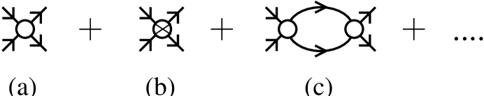
Figure 1: Lowest-order diagrams for the perturbative expansion of $T_{1}$. Particle propagators are represented by solid lines. The $C_{2}^{p}\,(C_{4}^{p})$ vertex is indicated by the open circle (crossed circle).

The result is simply

$$iT_{1(a)}=-iC_{2}^{p}\,{\mathbf{k}}\cdot{\mathbf{k}}^{\prime}\,.$$ (6)

The second term in the low-momentum expansion is suppressed by $k^{2}/M_{hi}^{2}$ compared to the leading order. It is given by the tree-level diagram with the $C_{4}^{p}$ interaction shown in Fig. 1(b):

$$iT_{1(b)}=-iC_{4}^{p}k^{2}\,{\mathbf{k}}\cdot{\mathbf{k}}^{\prime}\,.$$ (7)

At order $12\pi k^{5}/mM_{hi}^{6}$, we have the one-loop diagram with two $C_{2}^{p}$ interactions shown in Fig. 1(c). The contribution of this diagram is

$$iT_{1(c)} = (-iC_{2}^{p})^{2}\int\frac{d^{4}q}{(2\pi)^{4}}\frac{i\,{\mathbf{q}}\cdot{\mathbf{k}}}{\frac{E}{2}+q_{0}-\frac{{\mathbf{q}}^{2}}{2m}+i\epsilon}\frac{i\,{\mathbf{q}}\cdot{\mathbf{k}}^{\prime}}{\frac{E}{2}-q_{0}-\frac{{\mathbf{q}}^{2}}{2m}+i\epsilon}$$ (8)

$$= (C_{2}^{p})^{2}imk^{\prime}_{i}k_{j}\int\frac{d^{3}q}{(2\pi)^{3}}\frac{q_{i}q_{j}}{q^{2}-k^{2}-i\epsilon}\,.$$

where the $dq_{0}$ integral was performed via contour integration. The remaining integral must be proportional to $\delta_{ij}$ since no other vectors are available. Adding and subtracting $k^{2}$ in the numerator, we find

$$iT_{1(c)} = (C_{2}^{p})^{2}\frac{im}{6\pi^{2}}\,{\mathbf{k}}\cdot{\mathbf{k}}^{\prime}\,\left\{\int dq\,q^{2}+k^{2}\int dq+k^{4}\int dq\frac{1}{q^{2}-k^{2}-i\epsilon}\right\}\,,$$ (9)

$$= (C_{2}^{p})^{2}\frac{im}{6\pi^{2}}\,{\mathbf{k}}\cdot{\mathbf{k}}^{\prime}\,\left\{L_{3}+k^{2}L_{1}+\frac{\pi}{2}ik^{3}\right\}\,,$$

where $L_{3}$ and $L_{1}$ are infinite constants. These two ultraviolet divergent terms can be absorbed by redefining the low-energy constants $C_{2}^{p}$ and $C_{4}^{p}$, respectively, which are already present in $T_{1(a)}$ and $T_{1(b)}$. No new parameter enters at this order. The series proceeds in an obvious way.

We can now match to Eq. (3) to relate the renormalized coefficients to the effective-range parameters. We find from Eq. (6) that $C_{2}^{p}=12\pi a_{1}/m$, and from Eq. (7) that $C_{4}^{p}=C_{2}^{p}r_{1}a_{1}/2$. After renormalization, $T_{1(c)}$ reproduces the third term in the low-momentum expansion of Eq. (3). Note that diagram 1(c) cannot be renormalized by $C_{2}^{p}$ alone even though it does not contain a $C_{4}^{p}$ vertex. This observation has important consequences in the unnatural case with fine-tuning.

II.2 Unnatural Case

Now we turn to the more interesting case with a shallow $p$-wave state. In Refs. vKo99 ; KSW98 , it was shown that for a shallow $s$-wave state the leading-order contact interaction $C_{0}$ has to be treated nonperturbatively. In this case, $C_{0}$ is enhanced by a factor $M_{hi}/M_{lo}$ over the expectation $C_{0}\sim 4\pi/mM_{hi}$ from naive dimensional analysis. Adding a new rung in the ladder forming the amplitude means adding an intermediate state ($\sim mk/4\pi$) and a $C_{0}$ ($\sim 4\pi/mM_{lo}$). Since the physics of the bound state is determined by $k\sim M_{lo}$, $C_{0}$ has to be summed to all orders.

For $p$ waves matters are slightly more complicated. We have seen above that the renormalization of the one-loop diagram with two $C_{2}^{p}$ interactions requires tree-level counterterms corresponding to both the leading $C_{2}^{p}$ and subleading $C_{4}^{p}$ interaction. As consequence, at least the $C_{2}^{p}$ and $C_{4}^{p}$ interactions have to be treated nonperturbatively if a shallow $p$-wave state is present.

Bound (virtual) states are associated with poles in the $S$-matrix on the upper (lower) half of the complex momentum plane. The characteristic momentum $\gamma$ of the bound/virtual state is given by position of the pole, $|k|\equiv\gamma$. For a shallow $p$-wave state with $\gamma\sim M_{lo}$, the magnitude of both the effective range and the scattering length must be set by $M_{lo}$. This is a consequence of the renormalization argument from the previous subsection. Either $C_{2}^{p}$ and $C_{4}^{p}$ are both enhanced or they are both natural. Assuming that the higher terms in the effective range expansion are natural, the order of magnitude of the first three terms in the expansion is

$$k^{3}\cot\delta_{1}\sim M_{lo}^{3}+M_{lo}k^{2}+\frac{1}{M_{hi}}k^{4}+\ldots\,,$$ (10)

and the effective-range parameters scale as

$$\frac{1}{a_{1}}\sim M_{lo}^{3}\,,\quad\frac{r_{1}}{2}\sim M_{lo}\,,\quad\mbox{ and }\quad\frac{{\cal P}_{1}}{4}\sim\frac{1}{M_{hi}}\,.$$ (11)

Both $C_{2}^{p}$ and $C_{4}^{p}$ are enhanced over the expectation from naive dimensional analysis and scale as

$$C_{2}^{p}\sim\frac{12\pi}{mM_{lo}^{3}}\qquad\mbox{and}\qquad C_{4}^{p}\sim\frac{12\pi}{mM_{lo}^{5}}\,.$$ (12)

Consequently, for momenta of order $M_{lo}$ neither interaction can be treated perturbatively. The shape parameter ${\cal P}_{1}$, however, is of order $1/M_{hi}$ and its contribution is suppressed by $M_{lo}/M_{hi}$ compared to the leading order.

In the following, we will demonstrate that treating the $C_{2}^{p}$ and $C_{4}^{p}$ interactions to all orders is indeed sufficient for proper renormalization and, moreover, required to reproduce the physics of the shallow $p$-wave state. We will also work out the leading-order description of a shallow $p$-wave state.

For convenience, we will not use the Lagrangian (4) but follow Ref. Kap97 and introduce an auxiliary field (the dimeron) for the two-particle state. The corresponding Lagrangian is,

$${\cal L} = \psi^{\dagger}\biggl{[}i\partial_{0}+\frac{\overrightarrow{\nabla}^{\,2}}{2m}\bigg{]}\psi+\eta_{1}d^{\dagger}_{i}\bigg{(}i\partial_{0}+\frac{\overrightarrow{\nabla}^{\,2}}{4m}-\Delta_{1}\bigg{)}d_{i}+\frac{g_{1}}{4}\left(d^{\dagger}_{i}(\psi\tensor{\nabla}_{i}\psi)+{\rm H.c.}\right)+\ldots\,,$$ (13)

where the sign $\eta_{1}=\pm 1$ and the parameters $g_{1}$ and $\Delta_{1}$ will be fixed from matching. This Lagrangian contains exactly the same number of parameters as the original Lagrangian (4). Up to higher order terms, Eq. (13) is equivalent to Eq. (4), as can be seen by performing the Gaussian path integral over $d_{i}$.

The bare dimeron propagator is given by

$$iD_{1}^{0}(p_{0},{\mathbf{p}})_{ij}=\frac{i\eta_{1}\delta_{ij}}{p_{0}-{\mathbf{p}}^{2}/4m-\Delta_{1}+i\epsilon}\,.$$ (14)

Summing the $C_{2}^{p}$ and $C_{4}^{p}$ interactions to all orders in the theory without the dimeron corresponds to dressing the bare dimeron propagator with particle bubbles to all orders. This summation is shown diagrammatically in Fig. 2.

Figure 2: The full dimeron propagator (thick shaded line) is obtained by dressing the bare dimeron propagator (double solid line) with particle bubbles (solid lines) to all orders.

The full dimeron propagator is most easily calculated by first computing the self-energy from the particle bubble $-i\Sigma_{1}$ which up to overall factors is given by the one-loop diagram from Fig. 1(c). We have

$$-i\Sigma_{1}(p_{0},{\mathbf{p}})_{ij} = g_{1}^{2}\int\frac{d^{4}q}{(2\pi)^{4}}\frac{q_{i}q_{j}}{\left(\frac{p_{0}}{2}+q_{0}-\frac{({\mathbf{p}}/2+{\mathbf{q}})^{2}}{2m}+i\epsilon\right)\left(\frac{p_{0}}{2}-q_{0}-\frac{({\mathbf{p}}/2-{\mathbf{q}})^{2}}{2m}+i\epsilon\right)}$$ (15)

$$= i\delta_{ij}\frac{mg_{1}^{2}}{12\pi}\left\{\frac{2}{\pi}L_{3}+\frac{2}{\pi}L_{1}\left(mp_{0}-{\mathbf{p}}^{2}/4\right)+i\left(mp_{0}-{\mathbf{p}}^{2}/4\right)^{3/2}\right\},$$

where $L_{3}$ and $L_{1}$ are infinite constants as in Eq. (9). The full dimeron propagator now simply follows from the geometric series

$$iD_{1}(p_{0},{\mathbf{p}}) = iD_{1}^{0}(p_{0},{\mathbf{p}})+iD_{1}^{0}(p_{0},{\mathbf{p}})(-i\Sigma_{1}(p_{0},{\mathbf{p}}))iD_{1}^{0}(p_{0},{\mathbf{p}})+\ldots$$ (16)

$$= iD_{1}^{0}(p_{0},{\mathbf{p}})\left(1-\Sigma_{1}(p_{0},{\mathbf{p}})D_{1}^{0}(p_{0},{\mathbf{p}})\right)^{-1}\,,$$

where the vector indices have been suppressed. Using Eqs. (14, 15), we find

$$iD_{1}(p_{0},{\mathbf{p}})_{ij} = -i\delta_{ij}\frac{12\pi}{mg_{1}^{2}}\left(\frac{12\pi\Delta_{1}}{\eta_{1}mg_{1}^{2}}-\frac{12\pi}{\eta_{1}m^{2}g_{1}^{2}}\left(mp_{0}-{\mathbf{p}}^{2}/4\right)\right.$$

$$\qquad\qquad\left.-\frac{2}{\pi}L_{3}-\frac{2}{\pi}L_{1}\left(mp_{0}-{\mathbf{p}}^{2}/4\right)-i\left(mp_{0}-{\mathbf{p}}^{2}/4\right)^{3/2}\right)^{-1}\,,$$

$$= -i\delta_{ij}\frac{12\pi}{mg_{1}^{2}}\left(\eta_{1}\frac{12\pi\Delta_{1}^{R}}{m(g_{1}^{R})^{2}}-\eta_{1}\frac{12\pi}{m^{2}(g_{1}^{R})^{2}}\left(mp_{0}-{\mathbf{p}}^{2}/4\right)-i\left(mp_{0}-{\mathbf{p}}^{2}/4\right)^{3/2}\right)^{-1}\,,$$

where the last line defines the renormalized parameters $\Delta_{1}^{R}$ and $g_{1}^{R}$.

The $p$-wave scattering amplitude is obtained by attaching external particles lines to the full dimeron propagator. In the center-of-mass system, $(p_{0},{\mathbf{p}})=(k^{2}/m,{\mathbf{0}})$, this leads to

$$T_{1}(k,\cos\theta) = \frac{12\pi}{m}k^{2}\cos\theta\left(\eta_{1}\frac{12\pi\Delta_{1}}{m(g_{1}^{R})^{2}}-\eta_{1}\frac{12\pi}{m^{2}(g_{1}^{R})^{2}}k^{2}-ik^{3}\right)^{-1}$$ (18)

$$\equiv \frac{12\pi}{m}k^{2}\cos\theta\left(-\frac{1}{a_{1}}+\frac{r_{1}}{2}k^{2}-ik^{3}\right)^{-1}\,,$$

from which the matching conditions can be read off easily. We see that, as advertised, two coefficients are necessary and sufficient to remove any significant cutoff dependence.

II.3 Pole Structure

In this subsection, we discuss the pole structure of the $S$-matrix in the unnatural case. Neglecting terms suppressed by $M_{lo}/M_{hi}$, the equation determining the poles is, from the amplitude (18),

$$-\frac{1}{a_{1}}+\frac{r_{1}}{2}\kappa^{2}-i\kappa^{3}=0\,.$$ (19)

For definiteness, we concentrate on the case $a_{1},r_{1}<0$ that is relevant to $n\alpha$ scattering. Other cases can be examined as easily. The solutions are one pole $\kappa_{1}$ on the positive imaginary axis and two complex-conjugated poles in the lower half-plane. They have the structure

$$\kappa_{1}=i\gamma_{1}\qquad\mbox{and}\qquad\kappa_{\pm}=i(\gamma\pm i\tilde{\gamma})\,,$$ (20)

where

$$\gamma_{1} = \frac{1}{6}\left(|r_{1}|+\frac{|a_{1}|^{1/3}|r_{1}|^{2}}{v}+\frac{v}{|a_{1}|^{1/3}}\right)\,,$$

$$\gamma = \frac{1}{6}\left(|r_{1}|-\frac{|a_{1}|^{1/3}|r_{1}|^{2}}{2v}-\frac{v}{2|a_{1}|^{1/3}}\right)\,,$$

$$\tilde{\gamma} = -\frac{\sqrt{3}}{12}\left(\frac{|a_{1}|^{1/3}|r_{1}|^{2}}{v}-\frac{v}{|a_{1}|^{1/3}}\right)\,,$$

$$v = \left(108+|a_{1}||r_{1}|^{3}+108\sqrt{1+|a_{1}||r_{1}|^{3}/54}\right)^{1/3}\,.$$ (21)

This pole structure is illustrated in Fig. 3.

Figure 3: The pole structure of the $S$-matrix for a $p$-wave resonance.

This general structure remains qualitatively unchanged in the limit $|r_{1}|\to 0$.

The $p$-wave contribution to the $S$-matrix can be written as

$$S_{1}=e^{2i\delta_{1}}=-\frac{k+\kappa_{1}}{k-\kappa_{1}}\,\frac{k+\kappa_{+}}{k-\kappa_{+}}\,\frac{k+\kappa_{-}}{k-\kappa_{-}}=-\frac{k+i\gamma_{1}}{k-i\gamma_{1}}\,\frac{E-E_{0}-\frac{i}{2}\Gamma(E)}{E-E_{0}+\frac{i}{2}\Gamma(E)}\,,$$ (22)

where we have defined

$$E=\frac{k^{2}}{2\mu}\,,\qquad E_{0}=\frac{\gamma^{2}+\tilde{\gamma}^{2}}{2\mu}\qquad\mbox{and}\qquad\Gamma(E)=-4\gamma\sqrt{\frac{E}{2\mu}}\,,$$ (23)

with $\mu$ the reduced mass of the system. The phase shift can therefore be written as

$$\delta_{1}=\frac{1}{2i}\ln S_{1}=\delta_{s}(E)-\arctan\left(\frac{\Gamma(E)}{2(E-E_{0})}\right)\,.$$ (24)

Here

$$\delta_{s}(E)=\frac{1}{2}\arctan\left(\frac{2\sqrt{EB}}{E-B}\right)$$ (25)

is the contribution from the bound state with binding energy $B=\gamma_{1}^{2}/2\mu$. It changes by $\pi/2$ as the energy varies across $B$. $\delta_{s}(E)$ is a relatively smooth function of the energy $E$. The two complex-conjugated poles $\kappa_{\pm}$ generate the resonance that is given by the second term in Eq. (24). This term changes by $\pi$ as the energy varies across $E_{0}$.

In the case of $s$ waves, the EFT determines in leading order the position of a shallow real or virtual bound state. In the $p$ waves the physics is richer: the two leading-order parameters provide the position and width of a resonance (in addition to the position of a bound state).

III Application to Elastic $n\alpha$ Scattering

We are now in position to extend the EFT for shallow $p$-wave states from the previous section to the $n$-⁴He system, including the spin of the nucleon. We calculate the leading- and next-to-leading-order contributions to low-energy elastic $n\alpha$ scattering. First, we briefly review the structure of the cross section and scattering amplitude.

III.1 Cross Section and Scattering Amplitude

The differential cross section for elastic $n\alpha$ scattering in the center-of-mass frame can be written as

$$\frac{d\sigma}{d\Omega}=|F(k,\theta)|^{2}+|G(k,\theta)|^{2}\,,$$ (26)

where $k$ and $\theta$ are the magnitude of the momentum and the scattering angle, respectively. The so-called spin-no-flip and spin-flip amplitudes $F$ and $G$ can be expanded in partial waves as

$$F(k,\theta) = \sum_{l\geq 0}\left[(l+1)f_{l+}(k)+lf_{l-}(k)\right]P_{l}(\cos\theta)\,,$$ (27)

$$G(k,\theta) = \sum_{l\geq 1}\left[f_{l+}(k)-f_{l-}(k)\right]P^{1}_{l}(\cos\theta)\,,$$ (28)

where $P_{l}$ is a Legendre polynomial and

$$P_{l}^{1}(x)=(1-x^{2})^{1/2}\frac{d}{dx}P_{l}(x)\,.$$ (29)

The partial wave amplitudes $f_{l\pm}$ are related to the phase shifts $\delta_{l\pm}$ via

$$f_{l\pm}(k)=\frac{1}{2ik}\left[e^{2i\delta_{\pm}}-1\right]=\frac{1}{k\cot\delta_{l\pm}-ik}\,.$$ (30)

The total cross section can be obtained from the optical theorem,

$$\sigma_{T}=\frac{4\pi}{k}\,{\rm Im}\,F(k,0)\,.$$ (31)

The $T$-matrix calculated in EFT is related to the amplitudes $F$ and $G$ via

$$T=\frac{2\pi}{\mu}\left(F+i\mbox{\boldmath$\sigma$}\cdot\hat{{\mathbf{n}}}G\right)\,,$$ (32)

where $\mu=m_{\alpha}m_{N}/(m_{\alpha}+m_{N})$ is the reduced mass, $\hat{{\mathbf{n}}}={\mathbf{k}}\times{\mathbf{k}}^{\prime}/|{\mathbf{k}}\times{\mathbf{k}}^{\prime}|$ with ${\mathbf{k}}$ and ${\mathbf{k}}^{\prime}$ the initial and final momenta in the center-of-mass frame, and $\mbox{\boldmath$\sigma$}=(\sigma_{1},\sigma_{2},\sigma_{3})$ is a three-vector of the usual Pauli matrices.

For $n\alpha$ scattering at low energies only the $s$ and $p$ waves are important. There is one $s$ wave: $l\pm=0+$ with $l_{j}=s_{1/2}$, and two $p$ waves: $l\pm=1+$ and $1-$ corresponding to $l_{j}=p_{3/2}$ and $p_{1/2}$, respectively. In the remainder of the paper, we use the $l\pm$ notation for the partial waves. In Ref. ALR73 , a phase-shift analysis including the $0+$, $1-$, and $1+$ partial waves was performed and the effective-range parameters were extracted. The effective range expansion for a partial wave with orbital angular momentum $l$ was given in Eq. (2). The effective-range parameters extracted in Ref. ALR73 are listed in Table 1.

Partial wave $l_{\pm}$	$a_{l\pm}$ [fm1+2l]	$r_{l\pm}$ [fm1-2l]	${\cal P}_{l\pm}$ [fm3-2l]
$0+$	$2.4641(37)$	$1.385(41)$	$-$
$1-$	$-13.821(68)$	$-0.419(16)$	$-$
$1+$	$-62.951(3)$	$-0.8819(11)$	$-3.002(62)$

Table 1: The values of the scattering length $a_{l\pm}$, the effective range $r_{l\pm}$, and the shape parameter ${\cal P}_{l\pm}$ in elastic $n\alpha$ scattering for the $0+$, $1-$, and $1+$ partial waves from Ref. ALR73 . The numbers in parenthesis indicate the error in the last quoted digits. All values are given in units of the appropriate powers of fm as determined by the orbital angular momentum $l$ of the partial wave.

The $1+$ partial wave has a large scattering length and somewhat small effective range, as expected from Eq. (11). Indeed, the phase shift in this wave has a resonance corresponding to a shallow $p$-wave state ALR73 . As a consequence, the $1+$ partial wave has to be treated nonperturbatively using the formalism for shallow $p$-wave states developed in the previous section. In the $0+$ wave, on the other hand, the scattering length and effective range are clearly of natural size. The $0+$ partial wave can be treated in perturbation theory. The situation is less clear in the $1-$ wave. Although the pattern is similar to the $1+$ wave, the phase shifts in the $0+$ and $1-$ partial waves show no resonant behavior at low energies ALR73 . We therefore expect that perturbation theory can be applied to the $1-$ partial wave as well.

These points can be made slightly more precise. We can estimate the scales $M_{lo}$ and $M_{hi}$ from the effective-range parameters. Using the parameters for the $1+$ partial wave from Table 1, we find for $M_{lo}$ 50 MeV from the scattering length and 90 MeV from the effective range. The average value is $M_{lo}\approx 70$ MeV. From the shape parameter, we extract $M_{hi}\approx 260$ MeV. This is consistent with the hierarchy $M_{lo}\ll M_{hi}\sim m_{\pi}\sim\sqrt{m_{N}E_{\alpha}}$, where $E_{\alpha}=20.21$ MeV is the excitation energy of the $\alpha$ core tunl , and suggests that our power counting is appropriate for the $1+$ partial wave. We would expect that the scale of all effective-range parameters in the remaining channels is set by $M_{hi}$. Extracting the numbers, however, we find for $M_{hi}$ the scales 80 MeV from $a_{0+}$, 280 MeV from $r_{0+}$, 80 MeV from $a_{1-}$, and 40 MeV from $r_{1-}$. While some spread is not surprising given the qualitative nature of the argument, these numbers suggest that, even though the $1-$ phase shift is small, this partial wave might also be dominated by $M_{lo}$. For the moment we will assume this is not the case and treat the $1-$ wave in perturbation theory. We can certainly improve convergence by resumming $1-$ contributions. We return to this point in Sect. III.4.

III.2 Scattering Amplitude in the EFT

A real test of the power counting comes only by calculating the amplitude at various orders and comparing the results among themselves and with data. In the following, we will compute $n\alpha$ scattering to next-to-leading order in the EFT. For characteristic momenta $k\sim M_{lo}$, the leading-order contribution to the $T$-matrix is of order $12\pi/mM_{lo}$. The EFT expansion is in $M_{lo}/M_{hi}$ and the NLO and N²LO contributions are suppressed by powers of $M_{lo}/M_{hi}$ and $M_{lo}^{2}/M_{hi}^{2}$, respectively. The parameters in the effective Lagrangian will be determined from matching to effective-range parameters. We then compare our results with the phase-shift analysis ALR73 and also directly with low-energy data.

We represent the nucleon and the ⁴He core by a spinor/isospinor $N$ field and a scalar/isoscalar $\phi$ field, respectively. We also introduce isospinor dimeron fields that can be thought of as bare fields for the various $N\alpha$ channels. In the following we will employ $s$, $d$, and $t$, which are spinor, spinor and four-spinor fields associated with the $s_{1/2}$, $p_{1/2}$, and $p_{3/2}$ channels, respectively.

The parity- and time-reversal-invariant Lagrangians for LO and NLO are

$${\cal L}_{\rm LO} = \phi^{\dagger}\biggl{[}i\partial_{0}+\frac{\overrightarrow{\nabla}^{\,2}}{2m_{\alpha}}\bigg{]}\phi+N^{\dagger}\biggl{[}i\partial_{0}+\frac{\overrightarrow{\nabla}^{\,2}}{2m_{N}}\bigg{]}N+\eta_{1+}t^{\dagger}\bigg{[}i\partial_{0}+\frac{\overrightarrow{\nabla}^{\,2}}{2(m_{\alpha}+m_{N})}-\Delta_{1+}\bigg{]}t$$ (33)

$$+\frac{g_{1+}}{2}\bigg{\{}t^{\dagger}{\mathbf{S}}^{\dagger}\cdot\bigg{[}N\overrightarrow{\nabla}\phi-(\overrightarrow{\nabla}N)\phi\bigg{]}+{\rm H.c.}-r\bigg{[}t^{\dagger}{\mathbf{S}}^{\dagger}\cdot\overrightarrow{\nabla}(N\phi)+{\rm H.c.}\bigg{]}\bigg{\}}\,,$$

$${\cal L}_{\rm NLO} = \eta_{0+}s^{\dagger}\bigg{[}-\Delta_{0+}\bigg{]}s+g_{0+}\bigg{[}s^{\dagger}N\phi+\phi^{\dagger}N^{\dagger}s\bigg{]}+g_{1+}^{\prime}t^{\dagger}\bigg{[}i\partial_{0}+\frac{\overrightarrow{\nabla}^{\,2}}{2(m_{\alpha}+m_{N})}\bigg{]}^{2}t\,,$$ (34)

where $r=(m_{\alpha}-m_{N})/(m_{\alpha}+m_{N})$. The notation is analogous to that in Eq. (13). The $S_{i}$’s are the $2\times 4$ spin-transition matrices connecting states with total angular momentum $j=1/2$ and $j=3/2$. They satisfy the relations

$$S_{i}S_{j}^{\dagger}=\frac{2}{3}\delta_{ij}-\frac{i}{3}\epsilon_{ijk}\sigma_{k}$$

$$S_{i}^{\dagger}S_{j}=\frac{3}{4}\delta_{ij}-\frac{1}{6}\bigg{\{}J_{i}^{3/2},J_{j}^{3/2}\bigg{\}}+\frac{i}{3}\epsilon_{ijk}J_{k}^{3/2}\,,$$ (35)

where the $J_{i}^{3/2}$ are the generators of the $J=3/2$ representation of the rotation group, with

$$\bigg{[}J_{i}^{3/2},J_{j}^{3/2}\bigg{]}=i\epsilon_{ijk}J_{k}^{3/2}\,.$$ (36)

These Lagrangians generate contributions in the $1+$ and $0+$ partial waves. There are no contributions in N²LO, and the $1-$ partial wave enters first at N³LO.

The propagator for the $\phi$ field is

$$iS_{\phi}(p_{0},{\mathbf{p}})=\frac{i}{p_{0}-{\mathbf{p}}^{\,2}/2m_{\alpha}+i\epsilon}\,,$$ (37)

while the nucleon propagator is

$$iS_{N}(p_{0},{\mathbf{p}})_{\alpha\beta}^{ab}=\frac{i\delta_{\alpha\beta}\delta_{ab}}{p_{0}-{\mathbf{p}}^{\,2}/2m_{N}+i\epsilon}\,.$$ (38)

In Eq. (38), $\alpha$ and $\beta$ ($a$ and $b$) are the incoming and outgoing spin (isospin) indices of the nucleon, respectively. The bare propagator for the $1+$ dimeron is

$$iD^{0}_{1+}(p_{0},{\mathbf{p}})_{\alpha\beta}^{ab}=\frac{i\eta_{1+}\delta_{\alpha\beta}\delta_{ab}}{p_{0}-{\mathbf{p}}^{\,2}/2(m_{\alpha}+m_{N})-\Delta_{1+}+i\epsilon}\,,$$ (39)

with $\alpha$ and $\beta$ ($a$ and $b$) the incoming and outgoing spin (isospin) indices of the dimeron, respectively. Note that $\delta_{\alpha\beta}$ is a $4\times 4$ unit matrix, since the dimeron carries $j=3/2$. The bare propagator for the $0+$ is slightly different because its kinetic terms do not appear until higher order:

$$iD^{0}_{0+}(0,{\mathbf{0}})_{\alpha\beta}^{ab}=-\frac{i\eta_{0+}\delta_{\alpha\beta}\delta_{ab}}{\Delta_{0+}}\,,$$ (40)

with $\delta_{\alpha\beta}$ now a $2\times 2$ unit matrix. The bare propagator for the $1-$ dimeron is the same as for the $0+$ dimeron, with the index $0+$ replaced by $1-$ where appropriate.

The leading contribution to the $n\alpha$ scattering amplitude for $k\sim M_{lo}$ is of order $12\pi/mM_{lo}$ and comes solely from the $1+$ partial wave with the scattering-length and effective-range terms included to all orders. The next-to-leading order correction is suppressed by $M_{lo}/M_{hi}$ and fully perturbative. It consists of the correction from the shape parameter ${\cal P}_{1+}$ in the $1+$ partial wave and the tree-level contribution of the scattering length $a_{0+}$ in the $0+$ partial wave. The $1-$ partial wave still vanishes at next-to-leading order.

First, we calculate the leading-order $T$-matrix element $T^{\rm LO}$. As demonstrated for spinless fermions in the previous section, this is most easily achieved by first calculating the full dimeron propagator for the $1+$ dimeron and attaching the external particle lines in the end. Apart from the spin/isospin algebra, the calculation is equivalent to the one for spinless fermions that was discussed in detail in the previous section. The proper self energy is given by

$$-i\Sigma_{1+}(p_{0},{\mathbf{p}})_{\alpha\beta}^{ab} = g_{1+}^{2}\int\frac{d^{d}l}{(2\pi)^{d}}\frac{({\mathbf{l}}-r{\mathbf{p}}/2)_{i}(S_{i}^{\dagger})_{\beta\gamma}({\mathbf{l}}-r{\mathbf{p}}/2)_{j}(S_{j})_{\gamma\alpha}\delta_{ab}}{\left(\frac{p_{0}}{2}+l_{0}-\frac{({\mathbf{p}}/2+{\mathbf{l}})^{2}}{2m_{\alpha}}+i\epsilon\right)\left(\frac{p_{0}}{2}-l_{0}-\frac{({\mathbf{p}}/2-{\mathbf{l}})^{2}}{2m_{N}}+i\epsilon\right)}$$ (41)

$$= -ig_{1+}^{2}(S_{i}^{\dagger}S_{j})_{\beta\alpha}\delta_{ba}\int\frac{d^{d-1}l}{(2\pi)^{d-1}}\frac{({\mathbf{l}}-r{\mathbf{p}}/2)_{i}({\mathbf{l}}-r{\mathbf{p}}/2)_{j}}{p_{0}-(p^{2}/4+l^{2}-r{\mathbf{p}}\cdot{\mathbf{l}})/2\mu+i\epsilon}\,,$$

where we have performed the $dl_{0}$ integral via contour integration. Evaluating the remaining integral using dimensional regularization with minimal subtraction for simplicity, we obtain

$$\Sigma_{1+}(p_{0},{\mathbf{p}})_{\alpha\beta}^{ab}=-\delta_{\alpha\beta}\delta_{ab}\frac{g_{1+}^{2}\mu}{6\pi}\left[2\mu\left(-p_{0}+\frac{{\mathbf{p}}^{\,2}}{2(m_{\alpha}+m_{N})}-i\epsilon\right)\right]^{3/2}\,.$$ (42)

Using Eq. (16), the full dimeron propagator is then given by

$$iD_{1+}(p_{0},{\mathbf{p}})_{\alpha\beta}^{ab} = {i\eta_{1+}\delta_{\alpha\beta}\delta_{ab}}\left(p_{0}-\frac{{\mathbf{p}}^{\,2}}{2(m_{\alpha}+m_{N})}-\Delta_{1+}\right.$$ (43)

$$\qquad\left.+\frac{\eta_{1+}\mu g_{1+}^{2}}{6\pi}(2\mu)^{3/2}\left[-p_{0}+\frac{{\mathbf{p}}^{\,2}}{2(m_{\alpha}+m_{N})}-i\epsilon\right]^{3/2}+i\epsilon\right)^{-1}\,.$$

The leading-order $T$-matrix element in the center-of-mass system is obtained by setting $(p_{0},{\mathbf{p}})=(k^{2}/2\mu,{\mathbf{0}})$ and attaching external particles lines to the full dimeron propagator. This leads to

$$T^{\rm LO}(k,\cos\theta) = \frac{2\pi}{\mu}k^{2}(2\cos\theta+i\mbox{\boldmath$\sigma$}\cdot\hat{{\mathbf{n}}}\sin\theta)\left(\eta_{1+}\frac{6\pi\Delta_{1+}}{\mu g_{1+}^{2}}-\eta_{1+}\frac{6\pi}{\mu^{2}g_{1+}^{2}}\frac{k^{2}}{2}-ik^{3}\right)^{-1}\,.$$ (44)

Using Eqs. (2) and (27) to (32), we find the matching conditions

$$a_{1+}=-\eta_{1+}\frac{\mu g_{1+}^{2}}{6\pi\Delta_{1+}}\qquad\mbox{ and }\qquad{r_{1+}}=-\eta_{1+}\frac{6\pi}{\mu^{2}g_{1+}^{2}}\,,$$ (45)

which determine the parameters $g_{1+}$, $\Delta_{1+}$, and the sign $\eta_{1+}$ in terms of the effective-range parameters $a_{1+}$ and $r_{1+}$. Then,

$$F^{\rm LO}(k,\theta) = \frac{2k^{2}\cos\theta}{-1/a_{1+}+r_{1+}k^{2}/2-ik^{3}}\,,$$

$$G^{\rm LO}(k,\theta) = \frac{k^{2}\sin\theta}{-1/a_{1+}+r_{1+}k^{2}/2-ik^{3}}\,.$$ (46)

At next-to-leading order, we include all contributions that are suppressed by $M_{lo}/M_{hi}$ compared to the leading order. These contributions come from the shape parameter ${\cal P}_{1+}$ and the $s$-wave scattering length $a_{0+}$. Using the Lagrangian (33) and (34), we find for the $T$-matrix element:

$$T^{\rm NLO} = \frac{\eta_{0+}g_{0+}^{2}}{\Delta_{0+}}+\frac{3\pi g_{1+}^{\prime}}{2\mu^{3}g_{1+}^{2}}\frac{2\pi}{\mu}\frac{k^{6}(2\cos\theta+i\mbox{\boldmath$\sigma$}\cdot\hat{{\mathbf{n}}}\sin\theta)}{(-1/a_{1+}+r_{1+}k^{2}/2-ik^{3})^{2}}\,.$$ (47)

The first term in Eq. (47) corresponds to the scattering length in the $0+$ wave, while the second term corresponds to the $1+$ amplitude with the shape parameter treated as a perturbation. Using Eqs. (2) and (27) to (32), we find

$$a_{0+}=-\frac{\eta_{0+}g_{0+}^{2}\mu}{2\pi\Delta_{0+}}\qquad\mbox{ and }\quad{\cal P}_{1+}=\frac{6\pi g_{1+}^{\prime}}{\mu^{3}g_{1+}^{2}}\,.$$ (48)

Note that to this order $\eta_{0+}$, $g_{0+}$, and $\Delta_{0+}$ are not independent and only the combination appearing in Eq. (48) is determined. The next-to-leading-order pieces of $F$ and $G$ are then

$$F^{\rm NLO}(k,\theta) = -a_{0+}+\frac{{\cal P}_{1+}}{4}\frac{2k^{6}\cos\theta}{(-1/a_{1+}+r_{1+}k^{2}/2-ik^{3})^{2}}\,,$$

$$G^{\rm NLO}(k,\theta) = \frac{{\cal P}_{1+}}{4}\frac{k^{6}\sin\theta}{(-1/a_{1+}+r_{1+}k^{2}/2-ik^{3})^{2}}\,.$$ (49)

III.3 Phase Shifts and Cross Sections in the EFT

In order to see how good our expansion is, we need to fix our parameters. In principle we could determine the parameters by matching our EFT to the underlying EFT whose degrees of freedom are nucleons (and possibly pions and delta isobars), but no core. Unfortunately, calculations with the latter EFT have not yet reached systems of five nucleons Birareview . For the time being, we need to determine the parameters from data. For simplicity, we use the effective-range parameters from Table 1 together with Eqs. (45,48).

In Fig. 4, we show the phase shifts for elastic $n\alpha$ scattering in the $1+$ partial wave as a function of the neutron kinetic energy in the $\alpha$ rest frame.

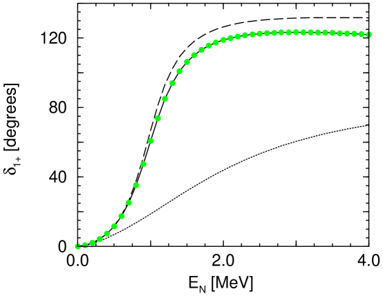
Figure 4: The phase shift for $n\alpha$ scattering in the $1+$ partial wave as a function of the neutron kinetic energy in the $\alpha$ rest frame. The dashed (solid) line shows the EFT result at LO (NLO). The filled circles show the phase-shift analysis ALR73 which the EFT at NLO reproduces exactly. The dotted line shows the contribution of the scattering length alone.

The filled circles show the phase-shift analysis of Ref. ALR73 . The dashed line shows the EFT result at leading order. The LO result already shows a good agreement with the full phase-shift analysis. As expected, the agreement deteriorates with energy. NLO corrections improve the agreement: the EFT result at NLO shown by the solid line reproduces the phase-shift analysis exactly. If better data were available and a more complete phase-shift analysis were performed, some small discrepancies would survive, to be remedied by higher orders.

The sharp rise in the $1+$ phase shift past $\pi/2$ denotes the presence of a resonance. To LO, the pole structure of the $S$-matrix is given in Sect. II.3. We find $\gamma_{1}=99$ MeV, $\gamma=-6$ MeV, and $\tilde{\gamma}=34$ MeV. Using Eq. (23), the position and width of the resonance are $E_{0}=0.8$ MeV and $\Gamma(E_{0})=0.6$ MeV, respectively. The two virtual states that produce the resonance are indeed at $|k|\sim M_{lo}$. The real bound state, for reasons that cannot be understood from the EFT itself, turns out numerically to be at considerably higher momentum, where the EFT can no longer be trusted. This is consistent with the known absence of a real ⁵He bound state.

We also illustrate in Fig. 4 an important aspect of the power counting. The dotted line shows the result from iterating $C_{2}^{p}$ alone. In other words, it is the contribution of the scattering length only. This curve, which would come from a naive application of the power counting for $s$ waves vKo99 ; KSW98 , does not correspond to any order in the power counting developed here, and clearly fails to describe the resonance near $E_{n}=1$ MeV.

In Fig. 5, we show the phase shifts for elastic $n\alpha$ scattering in the $0+$ partial wave as a function of the neutron kinetic energy in the $\alpha$ rest frame.

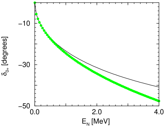
Figure 5: The phase shift for $n\alpha$ scattering in the $0+$ partial wave as a function of the neutron kinetic energy in the $\alpha$ rest frame. The solid line shows the EFT result at NLO; at LO this phase shift is zero. The filled circles show the result of the phase-shift analysis ALR73 .

In LO the phase shift is zero. The solid line shows the EFT result at next-to-leading order. The NLO result already shows good agreement with the full phase-shift analysis ALR73 , depicted by the filled circles.

The phase shifts in the $1-$ and all other partial waves are identically zero to NLO. The first non-zero contribution appears at N³LO in the $1-$ channel. All other waves appear at even higher orders. That they are indeed very small one can conclude from their absence in the phase-shift analysis ALR73 .

Obviously, not all partial waves are treated equally in our power counting. In order to further assess if the power counting is appropriate, we compare the EFT predictions directly to some observables. In Fig. 6, we compare the EFT predictions with data for the total cross section as a function of the neutron kinetic energy in the $\alpha$ rest frame.

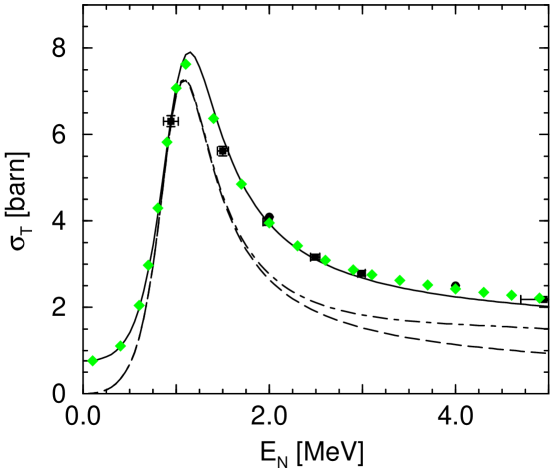
Figure 6: The total cross section for $n\alpha$ scattering in barns as a function of the neutron kinetic energy in the $\alpha$ rest frame. The diamonds are evaluated data from Ref. BNL , and the black squares are experimental data from Ref. data . The dashed and solid lines show the EFT results at LO and NLO, respectively. The dash-dotted line shows the LO result in the modified power counting where the $1-$ partial wave is promoted to leading order.

The diamonds are “evaluated data points” from Ref. BNL . In order to have an idea of the error bars from individual experiments we also show data from Ref. data as the black squares. The dashed line shows the EFT result at LO which already gives a fair description of the resonance region but underestimates the cross section at threshold. The NLO result given by the solid curve gives a good description of the cross section from threshold up to energies of about 4 MeV.

We can also calculate other observables. As another example, we show in Fig. 7 the center-of-mass differential cross section at a momentum $k_{CM}=49.6$ MeV. (This corresponds to a neutron kinetic energy $E_{n}=2.05$ MeV in the $\alpha$ rest frame.)

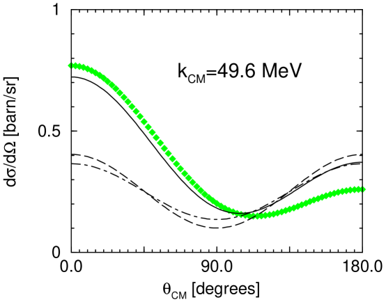
Figure 7: The differential cross section for $n\alpha$ scattering in the center-of-mass frame in barns/sr as a function of the scattering angle $\theta_{CM}$ at a momentum $k_{CM}=49.6$ MeV. The diamonds are evaluated data from Ref. BNL . The dashed and solid lines show the EFT results at LO and NLO, respectively. The dash-dotted line shows the LO result in the modified power counting where the $1-$ partial wave is promoted to leading order.

The diamonds are evaluated data from Ref. BNL . The dashed line show the EFT results at LO, which is pure $p$ wave. At NLO, shown as a solid line, interference with the $s$-wave term gives essentially the correct shape.

If we carry out the EFT to a sufficiently high order, we will have included all terms used in the phase-shift analysis ALR73 , and more. At this order, the high quality of our fit is purely a consequence of the high quality of that fit. Note, however, that this is by no means true at the lower orders explicitly displayed above. In particular, it is perhaps surprising that our $1-$ wave does not appear until relatively high order. The fact that the EFT converges fast to data shows that the power counting developed here is reasonable. The $1-$ wave is further discussed in the next section.

III.4 Further Discussion of the Power Counting

As we have shown, the EFT describes the data pretty well at least up to $E_{n}=4$ MeV or so. One way to improve the convergence at higher energies is to take the scale of non-perturbative phenomena in the $1-$ wave as a low scale. We can modify the power counting and count the $1-$ parameters the same as the $1+$ parameters. The LO Lagrangian from Eq. (33) then has an additional term

$${\cal L}_{\rm ALO} = \eta_{1-}d^{\dagger}\bigg{[}i\partial_{0}+\frac{\overrightarrow{\nabla}^{\,2}}{2(m_{\alpha}+m_{N})}-\Delta_{1-}\bigg{]}d$$ (50)

$$+ \frac{g_{1-}}{2}\bigg{\{}d^{\dagger}\mbox{\boldmath$\sigma$}^{\dagger}\cdot\bigg{[}N\overrightarrow{\nabla}\phi-(\overrightarrow{\nabla}N)\phi\bigg{]}+{\rm H.c.}-r\bigg{[}d^{\dagger}\mbox{\boldmath$\sigma$}^{\dagger}\cdot\overrightarrow{\nabla}(N\phi)+{\rm H.c.}\bigg{]}\bigg{\}}\,.$$

The calculation of the $T$-matrix for the $1-$ partial wave proceeds exactly as for the $1+$ partial wave. The amplitudes $F$ and $G$ acquire the following additional contributions at leading order

$$F^{\rm ALO}(k,\theta) = \frac{k^{2}\cos\theta}{-1/a_{1-}+r_{1-}k^{2}/2-ik^{3}}\,,$$

$$G^{\rm ALO}(k,\theta) = -\frac{k^{2}\sin\theta}{-1/a_{1-}+r_{1-}k^{2}/2-ik^{3}}\,.$$ (51)

In Fig. 8, we show the phase shifts for $n\alpha$ scattering in the $1-$ partial wave obtained in this alternative power counting.

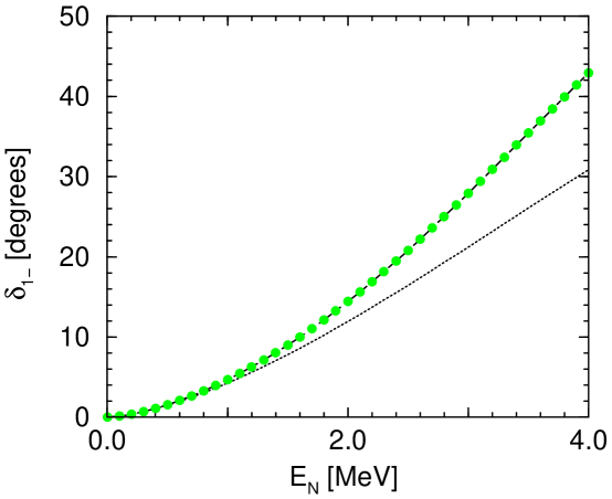
Figure 8: The phase shift for $n\alpha$ scattering in the $1-$ partial wave as a function of the neutron kinetic energy in the $\alpha$ rest frame. The filled circles show the result of the phase-shift analysis ALR73 which is exactly reproduced by leading-order EFT with the modified power counting given by the dash-dotted line. The dotted line shows the contribution of the scattering length only.

The filled circles show the result of the partial-wave analysis of Ref. ALR73 which is exactly reproduced by the leading-order EFT with the modified power counting given by the dash-dotted line. The dotted line shows the contribution of the scattering length only. The next-to-leading order in the modified counting cannot be easily computed at present because ${\cal P}_{1-}$ is not known.

The cross sections corresponding to the leading order in the modified power counting are shown by the dash-dotted curve in Figs. 6 and 7. In the total cross section, promoting the $1-$ partial wave to leading order gives almost no improvement compared to the original counting except at higher energies, but even there the NLO result in the original counting gives better results. In the differential cross section at $k_{CM}=49.6$ MeV (corresponding to $E_{n}=2.05$ MeV in the $\alpha$ rest frame), the alternative power counting gives no improvement over the LO result (compare the dashed and dash-dotted lines in Fig. 7). We did not find a significant improvement in the differential cross section over the leading order by promoting the $1-$ partial wave for neutron energies up to $E_{n}\approx 4$ MeV. For reproducing the differential cross section, the interference between $s_{1/2}$ and $p_{3/2}$ waves is much more important than the additional $p_{1/2}$ contribution. As a consequence, we deem the original power counting most appropriate for elastic $n\alpha$ scattering at $k\sim M_{lo}$.

Finally, note that for $k\ll M_{lo}$ the power counting has to discriminate between momentum $k$ and the low-energy scale $M_{lo}$. The $p$ waves, for example, die faster than the $s$ waves. That is the reason our results for the cross section in this region are not good until we get to NLO. It is easy to adapt the power counting for $k\ll M_{lo}$: in fact, the full amplitude —all waves, that is— can be treated in perturbation theory, as in Sect. II.1. For more details, see Ref. vKo99 .

IV Conclusion and Outlook

In this paper we have examined the problem of the interaction between a neutron and an $\alpha$ particle at low energies. We showed that a power counting can be formulated that leads to consistent renormalization. In leading order, two interactions have to be fully iterated. These two interactions generate a shallow $p_{3/2}$-wave resonance near the observed energy and width. In subleading orders the phase shifts in all waves can be systematically improved. Observables calculated directly are very well reproduced.

The crucial ingredient for the applicability of the EFT to bound states and resonances of halo type is their low characteristic energies. In this sense, the deuteron can be thought of as the simplest halo nucleus whose core is a nucleon. $n\alpha$ scattering plays an analogous role here as $np$ plays in the nucleons-only EFT. It is clear now how to extend the EFT to more complicated cores: one simply introduces an appropriate field for the core under consideration, extends the power counting to the relevant channels, and determines the strength of interactions order-by-order from data.

With the parameters of the nucleon-core interaction fixed in lowest orders, we can proceed to more-body halos. The simplest example is ⁶He. In addition to the $n\alpha$ interaction, the $nn$ interaction has also been determined from data. ⁶He, like the triton, can be described as a three-body system of a core and two neutrons. The role of a three-body interaction can be addressed by renormalization group techniques BHK99 ; ref6he .

Note that the EFT approach is by no means restricted to neutron halos. The Coulomb interaction can be included in the same way as in the nucleons-only sector em , allowing for the analysis of nuclei such as ⁸B. Radiative capture on halo nuclei, such as $p+\mbox{${}^{7}$Be}\to\mbox{${}^{8}$B}+\gamma$, can then be calculated much like $n+p\to d+\gamma$.

Our approach is not unrelated to traditional single-particle models. In the latter, the nucleon-core interaction is frequently parametrized by a simple potential with central and spin-orbit components potrev . The parameters of the potential are adjusted to reproduce whatever information is accessible experimentally. In the EFT, we make the equivalent to a multipole expansion of the underlying interaction. The spin-orbit splitting, in particular, results from the different parameters of the dimeron fields with different spins. In the EFT the nucleon-nucleon interaction is treated in the same way as the nucleon-core interaction, mutatis mutandis. Contact $NN$ interactions have in fact already been used in the study of Borromean halos george . It was found that density dependence, representing three-body effects, needed to be added in order to reproduce results from more sophisticated parametrizations of the $NN$ interaction. In the EFT, the need for an explicit three-body force can be decided on the basis of the renormalization group before experiment is confronted. A zero-range model with purely $s$-wave $NN$ and nucleon-core interactions was examined in Ref. tobiaselauro .

The EFT unifies single-particle approaches in a model-independent framework, with the added power counting that allows for an a priori estimate of errors. It also casts halo nuclei within the same framework now used to describe few-nucleon systems consistently with QCD Weinberg ; Birareview . Therefore, the EFT with a core can in principle be matched to the underlying, nucleons-only EFT. Nuclei near the drip lines open an exciting new field for the application of EFT ideas. It remains to be seen, however, whether these developments will prove to be a significant improvement over more traditional approaches.

References

- (1) B.A. Brown, A. Csótó, and R. Sherr, Nucl. Phys. A 597, 66 (1996); H. Esbensen and G.F. Bertsch, Nucl. Phys. A 600, 37 (1996).
- (2) M.V. Zhukov, B.V. Danilin, D.V. Fedorov, J.M. Bang, I.J. Thompson, and J.S. Vaagen, Phys. Rep. 231, 151 (1993); K. Riisager, Rev. Mod. Phys. 66, 1105 (1994).
- (3) Scientific Opportunities with Fast Fragmentation Beams from RIA, NSCL-Report (March 2000).
- (4) C.A. Bertulani, M.S. Hussein, and G. Münzenberg, Physics of Radioactive Beams (Nova Science Publishers, Huntington, NY, 2002).
- (5) G.P. Lepage, in From Actions to Answers, TASI’89, ed. T. DeGrand and D. Toussaint (World Scientific, Singapore, 1990); D.B. Kaplan, nucl-th/9506035.
- (6) P.F. Bedaque and U. van Kolck, Ann. Rev. Nucl. Part. Sci. (in press), nucl-th/0203055; S.R. Beane, P.F. Bedaque, W.C. Haxton, D.R. Phillips, and M.J. Savage, in Boris Ioffe Festschrift, ed. M. Shifman (World Scientific, Singapore, 2001).
- (7) Nuclear Physics with Effective Field Theory II, ed. P.F. Bedaque, M.J. Savage, R. Seki, and U. van Kolck (World Scientific, Singapore, 1999); Nuclear Physics with Effective Field Theory, ed. R. Seki, U. van Kolck, and M.J. Savage (World Scientific, Singapore, 1998).
- (8) S. Weinberg, Phys. Lett. B 251, 288 (1990); Nucl. Phys. B 363, 3 (1991); M. Rho, Phys. Rev. Lett. 66, 1275 (1991); C. Ordóñez and U. van Kolck, Phys. Lett. B 291, 459 (1992).
- (9) U. van Kolck, hep-ph/9711222, in Proceedings of the Workshop on Chiral Dynamics 1997, Theory and Experiment, ed. A. Bernstein, D. Drechsel, and T. Walcher (Springer-Verlag, Berlin, 1998); Nucl. Phys. A 645, 273 (1999).
- (10) D.B. Kaplan, M.J. Savage, and M.B. Wise, Phys. Lett. B 424, 390 (1998); Nucl. Phys. B 534, 329 (1998).
- (11) J.-W. Chen, G. Rupak, and M.J. Savage, Nucl. Phys. A 653, 386 (1999); S.R. Beane and M.J. Savage, Nucl. Phys. A 694, 511 (2001).
- (12) J.-W. Chen and M.J. Savage, Phys. Rev. C 60, 065205 (1999); G. Rupak, Nucl. Phys. A 678, 405 (2000).
- (13) P.F. Bedaque, H.-W. Hammer, and U. van Kolck, Phys. Rev. Lett. 82, 463 (1999); Nucl. Phys. A 646, 444 (1999).
- (14) P.F. Bedaque and U. van Kolck, Phys. Lett. B 428, 221 (1998); P.F. Bedaque, H.-W. Hammer, and U. van Kolck, Phys. Rev. C 58, R641 (1998); F. Gabbiani, P.F. Bedaque, and H.W. Grießhammer, Nucl. Phys. A 675, 601 (2000).
- (15) P.F. Bedaque, H.-W. Hammer, and U. van Kolck, Nucl. Phys. A 676, 357 (2000); H.-W. Hammer and T. Mehen, Phys. Lett. B 516, 353 (2001).
- (16) H.-W. Hammer, Nucl. Phys. A 705, 173 (2002).
- (17) D.V. Fedorov and A.S. Jensen, Nucl. Phys. A 697, 783 (2002).
- (18) C.A. Bertulani, H.-W. Hammer, and U. van Kolck, in preparation.
- (19) R.A. Arndt, D.L. Long, and L.D. Roper, Nucl. Phys. A 209, 429 (1973).
- (20) D.B. Kaplan, Nucl. Phys. B 494, 471 (1997).
- (21) D.R. Tilley, H.R. Weller, and G.M. Hale, Nucl. Phys. A 541, 1 (1992).
- (22) Evaluated Nuclear Data Files, National Nuclear Data Center, Brookhaven National Laboratory ( http://www.nndc.bnl.gov/ ).
- (23) B. Haesner et al., Phys. Rev. C 28, 995 (1983); M.E. Battat et al., Nucl. Phys. 12, 291 (1959).
- (24) X. Kong and F. Ravndal, Nucl. Phys. A 665, 137 (2000).
- (25) S. Ali, A.A.Z. Ahmad, and N. Ferdous, Rev. Mod. Phys. 57, 923 (1985).
- (26) G.F. Bertsch and H. Esbensen, Ann. Phys. 209, 327 (1991); H. Esbensen, G.F. Bertsch, and K. Hencken, Phys. Rev. C 56, 3054 (1997).
- (27) A.E.A. Amorim, T. Frederico, and L. Tomio, Phys. Rev. C 56, R2378 (1997); A. Delfino, T. Frederico, M.S. Hussein, and L. Tomio, Phys. Rev. C 61, 051301 (2000).