Introduction to Effective Field Theories in QCD

Abstract

We present a simple introduction to the techniques of effective field theory (EFT) and their application to QCD. For problems with more than one energy scale, the EFT approach is a useful alternative to more traditional model-building strategies. The most relevant such problem for this discussion is that of making contact between QCD and the hadronic phase of matter. As a simple example, an EFT calculation of the bound states of hydrogen within QED is sketched. A more significant demonstration of the power of EFTs, the construction of the chiral Lagrangian and chiral perturbation theory, is also included. The results provide us with the road map to a complete QCD-based theory of nuclear matter at nonzero temperatures and densities, a vital component to a quantitative understanding of the phase transition from hadron gas to quark-gluon plasma.

1 Introduction

Effective field theory (EFT) is a theoretical prescription for constructing theories spanning multiple energy scales. The physics of a system may appear radically different at different energy scales, due to low-energy restrictions on available degrees of freedom and symmetries. When trying to construct a theory which spans energy scales, traditional methods of physics can therefore be difficult to apply. Rather than stumbling on this obstacle, however, EFT provides a method to use the physical difference between energy regimes to advantage. We present an introduction to the basic ideas of this useful technique, from the perspective of its application to nuclear physics. The emphasis is pedagogical. Comprehensive and up-to-date reviews can be found in Ref. Bedaque (2002). For more extensive lectures with a similar perspective, the reader should refer to Ref. Phillips (2001).

In a typical experiment designed to produce a quark-gluon plasma (QGP), two heavy nuclei collide at relativistic speeds. The experimental signal that results is necessarily dependent not just on the nature of the plasma, but on the nature of the hadronic phase as well as the physics of the phase transformation. Trying to understand such an experiment with only an understanding of the plasma phase, therefore, is as doomed to failure as attempting to understand the latent heat of a water-to-steam transformation using only the kinetic theory of gases.

To remedy this problem, we must seek a true quantitative understanding of the physics of the hadronic phase. The theory we seek should furthermore be based on the microscopic theory of QCD. The development of theoretically-sound hadron interactions has been the major problem of nuclear physics since its inception. This theory must be valid over the significant temperatures and densities of the phase transformations typical in experiment. However, even a more limited approach that is restricted to the hadronic phase can be useful. One would like, for example, to estimate the position of the QGP transition line. Moreover, it is believed that the phase diagram of QCD presents other interesting features such a liquid-gas transition at lower temperatures and at densities close to that of equilibrium for cold nuclear matter.

At zero baryon density, an expansion in temperature $T$ of the free energy density of a pion gas can be derived in EFT and reveals the presence of a transition temperature $T_{c}$ at the point where the expansion diverges Gerber (1989). A more precise estimate can then be obtained by considering the effects of higher-mass mesons Rafelski (1980), in good agreement with lattice results Karsch (2000).

At non-zero baryon density $\rho$, on the other hand, the situation is much more complicated. Lattice QCD simulations are hampered by the infamous sign problem. EFT might therefore be the only way to study the problem, but it requires a conceptual leap from the work with mesons alone, because nucleons bind. Perturbative expansions for the energy density of dilute boson and fermion gases are well known: see, e.g., Ref. Braaten (1999) for $T=0$. These are expansions in $\rho a^{3}$, where $a$ is the scattering length, which is essentially the scattering amplitude at zero energy. The problem is that the nucleon-nucleon ($NN$) scattering length is large, so that the corresponding expansion fails way before the QGP phase transition. Indeed, the interesting physics of bound states such as nuclei is associated with $\rho^{1/3}$ $\stackrel{{\scriptstyle\textstyle>}}{{\sim}}$ $1/a$. The failure of a perturbative expansion in density implies that we must effectively resum such an expansion.

The reader may be somewhat surprised by the apparent failure in this regime of the perturbative approach, upon which so much of particle physics is based. This circumstance may be attributed to the complexities of the nonzero temperature and density requirements, as well as the striking disparities of the two energy scales we would like to connect. On the one hand, the consensus of the majority of the nuclear-physics community holds that in nuclei

• nucleons are non-relativistic;

• they interact via essentially two-body forces, with smaller contributions from many-body forces;

• the two-nucleon interaction generally possesses a high degree of isospin symmetry;

• external probes usually interact with mainly one nucleon at a time.

By contrast, in QCD

• the $u$ and $d$ quarks are relativistic;

• the interaction is manifestly multi-body, involving exchange of multiple gluons;

• there is no obvious isospin symmetry;

• external probes can, and often do, interact with many quarks at once.

It should not be surprising, then, that some new ideas are required to merge these two extraordinarily different bodies of theory. Of course, we expect that QCD encompasses the physics of hadronic interactions. The root of the problem must therefore lie in the difference of energy scales.

In fact, constructing a QCD-based theory of the hadronic phase is a problem which involves three separate energy scales spanning three orders of magnitude. The first and most obvious to a reader well versed in high-energy physics is the typical energy scale of QCD,

$$M_{QCD}\sim 1~{}\textrm{GeV}.$$ (1)

The masses of all hadrons except the pion fall within this scale , and the scale of chiral symmetry breaking is thought to be $M_{\chi}=4\pi f_{\pi}$, where $f_{\pi}\simeq 93$ MeV is the pion decay constant. The second scale,

$$M_{nuc}\sim 100~{}\textrm{MeV},$$ (2)

represents the typical momentum of nucleons in a nucleus: the inverse root-mean-square charge radius of light nuclei, or the Fermi momentum of equilibrium nuclear matter. It contains also the pion decay constant itself, the mass difference between the delta isobar and the nucleon, and the mass of the pion. The final energy scale is the typical energy scale of a nucleus,

$$\frac{M_{nuc}^{2}}{M_{QCD}}\sim 10~{}\textrm{MeV}.$$ (3)

The binding energy per nucleon of a nucleus is typically a few MeV. For example, the binding energy of ⁴He is 28.296 MeV, and the binding energy per nucleon of infinite nuclear matter is 16 MeV.

Since the goal is to construct a theory valid over an energy range of three orders of magnitude, and spanning regimes in which the physics is quite disparate, the problem is somewhat daunting. We might hope to seek inspiration from an analogous problem in atomic physics, the simple case of a hydrogen atom in the ground state. A qualitative argument suffices for this discussion. We know from experiment that the mass of an electron is

$$m_{e}\simeq 0.511~{}\textrm{MeV}.$$ (4)

The Hamiltonian is, to a good approximation, $H=p^{2}/2m_{e}-\alpha/r$, where $\alpha=e^{2}/4\pi\simeq 1/137$ is the fine-structure constant. From the uncertainty principle we know that the electron momentum is $p\sim 1/R$, if the size of the atom is $R$. Minimizing $E(R)=1/2m_{e}R^{2}-\alpha/R$ yields $R=1/\alpha m_{e}$, or

$$p\sim\alpha m_{e}=3.6~{}\textrm{keV}.$$ (5)

Finally, the binding energy $B=-E(1/\alpha m_{e})$ is

$$B\sim\frac{1}{2}\alpha^{2}m_{e}=13.6~{}\textrm{eV}.$$ (6)

This problem, like ours, possesses three distinct energy scales, on the order of $m_{e}$, $p$, and $B$. It is easy to see from the above, however, that in the atomic problem all three scales are coupled by the small fine-structure constant $\alpha$. It is not so clear what the analogous coupling constant should be in the nuclear problem. In fact, the lack of a clear small coupling constant is one of the main difficulties of nuclear physics. Even though our problem involves QCD, the strong coupling strength $\alpha_{s}$ is not useful to us, for at the highest energy scale in the problem $\alpha_{s}(1\textrm{GeV})\approx 1$ and perturbative QCD, valid at larger energies, breaks down.

If all obvious coupling parameters are of order one in the regime of our problem, we have no choice but to seek an alternative formulation. What is required is a theoretical framework that has the ability to sensibly and efficiently deal with multiple energy scales, as the perturbative approach does, but one that also does not rely ab initio on the existence of a small coupling constant. The framework which possesses both of these characteristics is EFT, as we shall see.

2 Effective Field Theory

EFT is a technique for developing theories of problems with multiple energy scales. It is applicable in situations where we wish to understand the physics at some low-energy scale as the limiting case of a more general problem whose full features are apparent only at some higher energy.

For simplicity, consider a generic problem with two energy scales. The complete physics of the problem throughout the full spectrum of energies can be said to be described by some Lagrangian density $\mathcal{L}\,(\varphi)$ in terms of some degrees of freedom $\varphi$. At a characteristic energy scale $E_{under}$, the full properties of $\mathcal{L}$ are vital to an understanding of the physics. In general, we may or may not know $\mathcal{L}$. Even if we know $\mathcal{L}$, we may or may not be able to solve it for the dynamics of the underlying theory. In our problem of the hadronic phase, for example, $\mathcal{L}$ is the QCD Lagrangian, and the underlying, full physics would be QCD. Processes explicitly involving quarks and gluons are seen to be important at energies of order $E_{under}\approx M_{QCD}$. At significantly lower energies, however, these processes “freeze out” and only hadronic degrees of freedom are available to the system. In the EFT, we therefore set some energy cutoff $\Lambda$ which divides energies of order $E_{under}$ from energies at which some of the freedoms of the full Lagrangian can be neglected.

The $S$-matrix contains all of the information relating initial states to final states in a many-body problem. The elements of the matrix can be calculated from the path integral

$$Z=\int\mathcal{D}\varphi e^{i\int\mathrm{d}^{D}x\mathcal{L}(\varphi)},$$ (7)

where $D$ is the number of spacetime dimensions in the problem. This expression is based in the full physics of the elementary, microscopic theory contained in $\mathcal{L}$.

We can begin to exploit the differences in physics between the two energy scales by using $\Lambda$ to relabel the fields according to momentum,

$$\varphi=\left\{\begin{array}[]{ll}\varphi_{H}&(p>\Lambda)\\ \varphi_{L}&(p<\Lambda),\end{array}\right.$$ (8)

and integrating over the degrees of freedom in $\varphi_{H}$. This gives us

$$Z=\int\mathcal{D}\varphi_{L}\int\mathcal{D}\varphi_{H}e^{i\int\mathrm{d}^{D}x\mathcal{L}(\varphi_{L},\varphi_{H})}=\int\mathcal{D}\varphi_{L}e^{i\int\mathrm{d}^{D}x\mathcal{L}_{eff}(\varphi_{L})},$$ (9)

where $\mathcal{L}_{eff}$ is defined by

$$\int\mathrm{d}^{D}x\,\mathcal{L}_{eff}(\varphi_{L})=-i\ln\int\mathcal{D}\varphi_{H}e^{i\int\mathrm{d}^{D}x\mathcal{L}(\varphi_{L},\varphi_{H})}.$$ (10)

$\mathcal{L}_{eff}$ is obviously a function only of $\varphi_{L}$, since we have integrated over $\varphi_{H}$. We can create a series representation for Eq. (10),

$$\int\mathrm{d}^{D}x\,\mathcal{L}_{eff}(\varphi_{L})\equiv\int\mathrm{d}^{D}x\sum_{i}g_{i}O_{i}(\varphi_{L}).$$ (11)

In general, Eq. (11) is a pure mathematical statement without any real physical content, but it becomes more meaningful when we make some statements about the properties of the operators $O_{i}$ and coefficients $g_{i}$.

The operators $O_{i}$ can in general be quite complicated. We can see, however, that they must possess two important physical properties. The first is that, although they contain an arbitrary number of derivatives, the $O_{i}$’s are in fact local operators in the sense that they involve fields at the same spacetime point. Nevertheless, their necessary dependence on derivatives follows from the fact that they depend only on fields with momentum components below $\Lambda$. As such, the uncertainty principle tells us that the operators can probe length scales only down to a minimum distance $\sim 1/\Lambda$, and so high-order derivatives will be necessary to perform the averaging over smaller length scales. The idea is the same as that of a multipole expansion in electrodynamics. The second observation we can make regarding the $O_{i}$’s is that, for an appropriate decomposition (8), they must possess all of the symmetries and transformation properties of the underlying high-energy theory. Even if a particular symmetry is broken, it will manifest itself in the same way in the effective Lagrangian.

The coefficients $g_{i}$ can likewise be put in perspective with some physical arguments. It is clear that they reflect the “freeze out” of the high-energy degrees of freedom below the cutoff $\Lambda$. Therefore, it is true that their particular form is dependent on the nature of the underlying theory and the structure of $\mathcal{L}\,(\varphi_{L},\varphi_{H})$. Furthermore, they are obviously a function of the cutoff parameter $\Lambda$. Note, however, that the specific dependence of the $g_{i}$ on $\Lambda$ is constrained by the familiar principle of renormalization-group invariance: physical observables cannot depend on the cutoff because the choice of the latter is arbitrary.

The physical motivation for EFT should now be apparent. It is an extremely common circumstance in physics that we wish to treat some low-energy limit of a fundamentally higher-energy problem. In such a case, we expect that the low-energy physics will prove to be some reflection of the full problem, but with the phase space restricted such that high-energy excitations or degrees of freedom are not accessible. Indeed, this is arguably the case in any physical problem short of a theory of everything: there exists some smaller-length and higher-energy scale at which new physics occurs, but whose details are unimportant to a description of a particular system. Were this not the case, physics as we know it would be impossible. The power of EFT, then, is that not only does it provide a framework to unify a problem with the energy scale above it, but it turns the energy difference from an obstacle into part of the solution: it recognizes this principle of limiting the system’s freedom at low energy and incorporates it directly into the theoretical strategy.

The EFT is useful even when we know and can solve the underlying theory at higher energies. In this case, it is possible to derive the coefficients $g_{i}$ from our knowledge of the underlying Lagrangian $\mathcal{L}\,(\varphi)$. The advantage lies in the reorganization of the dynamics in the EFT, as it is often the case that the effective degrees of freedom are “collective” excitations of the underlying degrees of freedom. This is the case whenever there is spontaneous breaking of a continuous symmetry and Goldstone bosons appear. An example is magnons, which are a better way to describe low-energy excitations in a system with spontaneous magnetization than individual magnetic moments. Another example are pions in QCD.

But EFT is a necessity when either the underlying theory is not known or, as in the case of QCD, it is not currently solvable. In this case, we can rely on Weinberg’s “theorem”: “if one writes down the most general possible Lagrangian, including all terms consistent with assumed symmetry principles, and then calculates $S$-matrix elements with this Lagrangian to any order in perturbation theory, the result will simply be the most general possible $S$-matrix consistent with analyticity, perturbative unitarity, cluster decomposition and the assumed symmetry principles” Weinberg (1979). There is no known general proof of this “theorem”, although it has been proven for a scalar field with $Z_{2}$ symmetry in Euclidean space Ball (1994). Nevertheless, it is certainly plausible, as it is really stating that the most general quantum field theory is a direct consequence only of analyticity, unitarity, cluster decomposition, and symmetry. This, combined with the fact that there are no known counterexamples, suggests that we would do well to consider the ramifications of the “theorem” regardless of its current lack of rigor.

Weinberg’s “theorem” allows us to formulate a plan to solve problems with an unknown or insoluble Lagrangian by using EFT.

1. Identify the relevant degrees of freedom and symmetries of the problem.

2. Construct the most general Lagrangian consistent with these limitations.

3. Do standard quantum field theory with this Lagrangian.

“Standard quantum field theory” consists of computing the contributions from all diagrams with momenta $Q<\Lambda$, and then renormalizing the result to relate the coefficients $g_{i}$ to the physical observables of the problem. After renormalization, observables should be independent of $\Lambda$. According to Weinberg’s “theorem”, these steps give the dynamics of the general system, and the process of building an EFT will have introduced no spurious information.

An important issue is that of ordering the infinite number of contributions to any observable, known as “power counting”. The minimal assumption is that, barring a suppression by some symmetry, the coefficients in the expansion will be roughly of ${\cal O}(1)$ once expressed in units of $E_{under}$ according to dimensional analysis. This is called the assumption of “naturalness”, and its validity is a consequence of our having chosen an appropriate cutoff $\Lambda$. The perturbative result of this process is a controlled expansion in energy, $E/E_{under}$. However, since observables are cutoff independent, the same expansion is valid for any cutoff. As we vary the cutoff, strength moves from one contribution to another that appears at the same order in $E/E_{under}$. So, regardless of the cutoff, to any given order in $E/E_{under}$ only a finite number of $g_{i}$’s need to be considered. One can use a finite number of experimental data as input to determine these $g_{i}$’s, and then use the known $g_{i}$’s to predict everything else, with an error given by the estimated size of higher-order terms. Thus, the most important ingredient to the final stage of building the EFT is power counting.

The controlled, natural expansion resulting from an EFT can be contrasted favorably with the characteristics of a theory constructed with traditional model-building strategies. A successful model takes a complex problem and reduces it reasonably to only a few degrees of freedom and types of interactions. This is a valid way to build a physical understanding of the problem, in that it allows the identification of the important symmetries and degrees of freedom. It falls short in quantitative predictive power, however, because there is no way to place a bound on the error arising from effects not included in the model. EFT, on the other hand, provides a controlled expansion of the most general dynamics, so errors are well bounded and predictable. The value of such an advantage in comparing theoretical predictions to experiment cannot be overstated.

2.1 A classical example

At this point, some simple examples of EFT calculations will prove fruitful. We begin with a problem drawn from classical physics, a light object interacting via gravity with a much larger object, for example an apple near the surface of the earth. We can easily identify the relevant degree of freedom and symmetries of this simple problem. By experimenting with various objects close to the surface of the earth, we find that, to a good approximation, the degree of freedom is the mass $m$, while the symmetries involve translations parallel to the earth’s surface and rotations about an axis normal to it. According to our recipe for an effective theory, we write down the most general potential reflecting these properties which is a power series in the height $h$:

$$V_{eff}(h)=m\sum_{i=0}^{\infty}g_{i}h^{i}.$$ (12)

Each of the $g_{i}$’s are parameters that can be fit to experimental data. (Here we are of course neglecting any quantum corrections, so there are no terms which are non-analytic in $h$ and $V_{eff}$ is directly observable.) The first term is an irrelevant constant that depends on the arbitrary choice of the zero in energy. The second term is the familiar $mgh$, where $g$ is the acceleration of a free body due to gravity as measured at $h=0$. The linear form of the gravitational potential, however, is simply an approximation: higher-order terms are corrections that could in principle be extracted from careful measurements. This expansion will breakdown at some energy $E_{under}$, which can be used to define a distance scale $R$ through $E_{under}\equiv mgR$. This is a controlled expansion in $h$ suitable for the low-energy regime $E\ll E_{under}$. The assumption of naturalness means

$$\frac{mg_{i+1}h^{i+1}}{mg_{i}h^{i}}=c_{i}\frac{E}{E_{under}}=c_{i}\frac{h}{R},$$ (13)

where the $c_{i}$’s are coefficients of ${\cal O}(1)$. This reduces to

$$g_{i+1}={\cal O}\left(\frac{g}{R^{i}}\right).$$ (14)

Thanks to Newton’s consideration of large distances, in this case we know the underlying theory. A more accurate expression for the gravitational potential follows from Newton’s law of universal gravitation,

$$V(h)=-GMm\frac{1}{R+h},$$ (15)

where $G$ is the gravitational constant, $M$ is the mass of the earth, and $R$ is its radius. For small $h$, we can expand Eq. (15) as

$$V(h)=mgR\sum_{i=0}^{\infty}(-1)^{i-1}\left(\frac{h}{R}\right)^{i},$$ (16)

where we have simplified the notation with the relation $g\equiv GM/R^{2}$. The underlying potential (16) indeed gives the effective gravitational potential (12) for $h\ll R$. Matching the two expressions, the coefficients of the effective potential are easily seen to be

$$g_{i+1}=(-1)^{i}\frac{g}{R^{i}}.$$ (17)

The naturalness assumption (14) is verified —all of the $c_{i}$’s are $\pm 1$— with the added understanding of the scale $R$ as the earth’s radius.

We have seen that the familiar linear form of gravitational potential energy can be treated as an effective theory of the more general theory given by Newton’s law of gravitation. It is worth noting in passing, however, that Newton’s law could also be viewed as an effective theory of a general relativistic formulation of gravitation whose effects are only visible at even larger energies. Thus, we can begin to develop a picture of nature as an “onion”, with each successively smaller energy scale being described by an effective theory of the last.

2.2 Non-relativistic QED

While a simple example from classical mechanics is instructive, we are now ready to increase our insight into the nature of EFT by examining a quantum-mechanical problem that bring us closer to our nuclear-physics interest. Let us attempt to find the effective Lagrangian for QED at low energies.

Consider fermions described by a field $\psi$ of mass $m$ and charge $e$, and assume the underlying theory to be given by the QED Lagrangian

$$\mathcal{L}_{QED}=\overline{\psi}[i(\not{\!\partial}-ie\not{\!\!A})-m]\psi+\frac{1}{4}F_{\mu\nu}F^{\mu\nu},$$ (18)

where $A_{\mu}$ ($F_{\mu\nu}$) is the photon field (field strength).

What happens in processes where all particles have momenta of the same order $Q\ll m$? Consider the part of a diagram found in Fig. 1, where the fermion interacts with a low-energy photon, either real or virtual. In this non-relativistic regime we can write

$$|\vec{p}|\sim|\vec{q}|\sim Q\ll m,$$ (19)

$$p^{0}=\sqrt{\vec{p}^{2}+m^{2}}\sim m+{\cal O}\left(\frac{Q^{2}}{m}\right),$$ (20)

$$q^{0}\sim|\vec{q}|\sim Q.$$ (21)

The internal fermion line (with momentum $p+q$) contributes a factor to these diagrams

$$\frac{i}{\not{\!\!p}+\not{\!q}-m+i\epsilon} = \frac{i(\not{\!\!p}+\not{\!q}+m)}{(p^{0}+q^{0})^{2}-(\vec{p}+\vec{q})^{2}-m^{2}+i\epsilon}$$ (22)

$$= \frac{i(\not{\!\!p}+\not{\!q}+m)}{{p^{0}}^{2}+2q^{0}p^{0}+{q^{0}}^{2}-(\vec{p}+\vec{q})^{2}-m^{2}+i\epsilon}$$

$$= \frac{i(\not{\!\!p}+m)}{2p^{0}q^{0}+i\epsilon}+\ldots=\frac{i}{q^{0}+i\epsilon}\frac{1+\gamma^{0}}{2}+\ldots$$

Here “$\ldots$” stand for terms which are suppressed by powers of $Q/m$.

Figure 1: Schematic representation of a class of processes involving a low-momentum fermion. The fermion first interacts with a real or virtual photon and then propagates until it interacts further.

The last equality in Eq. (22) contains the operator we will call $P_{+}$, which can be defined together with the complementary $P_{-}$,

$$P_{\pm}\equiv\frac{1\pm\gamma^{0}}{2}.$$ (23)

It is easy to verify that these operators possess the properties of idempotent projection operators:

$$P_{\pm}^{2}=P_{\pm},\;\;P_{\pm}P_{\mp}=0.$$ (24)

The presence of $P_{+}$ in Eq. (22) indicates that the fermion propagation is given by the particle propagating forward in time. This suggests that we separate the nearly-inert mass $m$ and the antiparticle component from the field, by rewriting the $\psi$ in a “heavy-fermion formalism” Georgi (1990)

$$e^{-imt}\smash[b]{\underset{\sim}{\smash[b]{\psi}}}_{\pm}\equiv P_{\pm}\psi.$$ (25)

The Lagrangian then becomes

$$\mathcal{L}_{QED}=\overline{\smash[b]{\underset{\sim}{\smash[b]{\psi}}}}_{+}i\partial_{0}\smash[b]{\underset{\sim}{\smash[b]{\psi}}}_{+}-\overline{\smash[b]{\underset{\sim}{\smash[b]{\psi}}}}_{-}i\vec{\gamma}\cdot\vec{\nabla}\smash[b]{\underset{\sim}{\smash[b]{\psi}}}_{+}+(\overline{i\vec{\gamma}\cdot\vec{\nabla}\smash[b]{\underset{\sim}{\smash[b]{\psi}}}_{-}})\smash[b]{\underset{\sim}{\smash[b]{\psi}}}_{+}+\overline{\smash[b]{\underset{\sim}{\smash[b]{\psi}}}}_{-}(-i\partial_{0}-2m)\smash[b]{\underset{\sim}{\smash[b]{\psi}}}_{-}+\ldots$$ (26)

We calculate the low-energy Lagrangian from Eq. (10). Completing the square, doing the gaussian integral over $\smash[b]{\underset{\sim}{\smash[b]{\psi}}}_{-}$, and renaming $\smash[b]{\underset{\sim}{\smash[b]{\psi}}}_{+}$ to $\psi$ yields

$$\mathcal{L}_{eff}\,(\psi)=\overline{\psi}i(\partial_{0}-ieA_{0})\psi+\frac{1}{2m}\overline{\psi}(\vec{\nabla}-ie\vec{A})^{2}\psi+\ldots+\frac{1}{4}F_{\mu\nu}F^{\mu\nu}+\ldots$$ (27)

Of course, in the real world, there exist more than one particle coupling to photons, and other gauge bosons coupling to these particles. Because the photon is massless while weak bosons are not, the latter can be integrated out at low energies. Likewise, we can integrate out other, heavier fermions. This results in additional terms in the effective Lagrangian, such as a Pauli term that gives rise to an anomalous magnetic moment through a parameter $\kappa$:

$$\mathcal{L}_{eff}^{(\mathrm{higher})}\,(\psi)=\frac{e}{2m}\kappa\varepsilon_{ijk}\overline{\psi}\sigma_{k}\psi F_{ij}+\ldots$$ (28)

The new parameters can be calculated from the underlying theory. All interactions in $\mathcal{L}_{eff}^{(\mathrm{higher})}$ are suppressed by powers of a heavy mass. The Pauli term, for example, is $\propto 1/m$, and $\kappa$ is of ${\cal O}(1)$ unless the particle represented by $\psi$ has only weak interactions.

Now, according to Weinberg’s “theorem”, we do not need to go through this whole song and dance. If we directly construct the most general effective Lagrangian involving the fermion $\psi$ and photon $A$ that is invariant under gauge transformations, parity, time reversal, and (non-relativistic) Lorentz boosts, we find the $\mathcal{L}_{eff}$ above.

2.3 Bound states in QED

With the above effective Lagrangian, we can return to the problem of the hydrogen atom, considered in the Introduction. We have already seen that this problem possesses multiple energy scales, much like the nuclear-physics problem we wish to solve. Discussing non-relativistic bound states in QED is a good warm-up for tackling nuclear bound states.

For simplicity, let us consider the interaction of two non-relativistic fermions of the same type. We denote the initial (final) center-of-mass momentum $p$ ($p^{\prime}$), with $|\vec{p}|\sim|\vec{p}^{\prime}|\sim Q$ and $p^{0}\sim{p^{\prime}}^{0}\sim Q^{2}/2m$. Since heavy-fermion number is conserved, all diagrams that contribute to the scattering amplitude $T$ have two fermion lines that go through. Let us consider first the diagrams made of photon exchange only, that is, of the type in Fig. 2, where the photon-fermion vertex comes from the first term in the Lagrangian (27). We want to estimate each to leading order in $Q$.

Figure 2: Diagrams representing all photon-exchange interactions between two heavy fermions in the center of momentum frame. The interaction $T$ is shorthand for all interactions which can occur. Note that $\ell$ is a dummy 4-momentum, and as such should be integrated over in the two loop diagrams.

The first-order diagram contributes a term

$$T^{(1)} = \frac{e^{2}}{(p-p^{\prime})^{2}+i\varepsilon}=\frac{e^{2}}{(p^{0}-{p^{\prime}}^{0})^{2}-(\vec{p}-\vec{p}^{\prime})^{2}+i\varepsilon}=-\frac{e^{2}}{(\vec{p}-\vec{p}^{\prime})^{2}-i\varepsilon}+\ldots$$ (29)

$$\sim\frac{e^{2}}{Q^{2}}.$$

The second-order term in which the photon lines cross is

$$T^{(2)(\times)}=-ie^{4}\int\frac{\mathrm{d}^{4}\ell}{(2\pi)^{4}}\frac{1}{p^{0}+\ell^{0}-\frac{(\vec{\ell}+\vec{p})^{2}}{2m}+i\varepsilon}\times\frac{1}{p^{\prime 0}+\ell^{0}-\frac{(\vec{\ell}-\vec{p}^{\prime})^{2}}{2m}+i\varepsilon}\\ \times\frac{1}{(p^{0}-{p^{\prime}}^{0}+\ell^{0})^{2}-(\vec{p}-\vec{p}^{\prime}+\vec{\ell})^{2}+i\varepsilon}\times\frac{1}{{\ell^{0}}^{2}-{\vec{\ell}}^{2}+i\varepsilon}.$$ (30)

The integral in $\ell^{0}$ can be evaluated as usual with a contour integral. It is clear that the first and second factors possess poles below the real axis, while the third and fourth terms each produce a pole above and below the real axis. We therefore minimize the algebra by closing in an infinite semicircle above the real axis: this way we avoid the two shallow poles from the nucleon propagators, and

$$\begin{split}T^{(2)(\times)}=e^{4}\int\frac{\mathrm{d}^{3}\ell}{(2\pi)^{3}}\frac{1}{p^{0}-|\vec{\ell}|-\frac{(\vec{\ell}+\vec{p})^{2}}{2m}+i\varepsilon}\times\frac{1}{p^{\prime 0}-|\vec{\ell}|-\frac{(\vec{\ell}-\vec{p}^{\prime})^{2}}{2m}+i\varepsilon}\\ \times\frac{1}{(p^{0}-{p^{\prime}}^{0}-|\vec{\ell}|)^{2}-(\vec{p}-\vec{p}^{\prime}+\vec{\ell})^{2}+i\varepsilon}\times\frac{1}{2|\vec{\ell}|-i\varepsilon}+\ldots\\ \end{split}$$

$$\sim e^{4}\Big{(}\frac{Q^{3}}{4\pi}\Big{)}\Big{(}\frac{1}{Q}\Big{)}\Big{(}\frac{1}{Q}\Big{)}\Big{(}\frac{1}{Q^{2}}\Big{)}\Big{(}\frac{1}{Q}\Big{)}\sim\alpha\frac{e^{2}}{Q^{2}}.$$ (31)

There is no surprise here: these contributions are, as ordinarily expected from loop diagrams, down by a factor of $\alpha$ compared to Eq. (29).

Life is not so boring, fortunately. In the other second-order term, the photon lines do not cross. This contributes

$$T^{(2)(=)}=-ie^{4}\int\frac{\mathrm{d}^{4}\ell}{(2\pi)^{4}}\frac{1}{p^{0}+\ell^{0}-\frac{(\vec{\ell}+\vec{p})^{2}}{2m}+i\varepsilon}\times\frac{1}{p^{0}-\ell^{0}-\frac{(\vec{\ell}+\vec{p})^{2}}{2m}+i\varepsilon}\\ \times\frac{1}{(p^{0}-{p^{\prime}}^{0}+\ell^{0})^{2}-(\vec{p}-\vec{p}^{\prime}+\vec{\ell})^{2}+i\varepsilon}\times\frac{1}{{\ell^{0}}^{2}-{\vec{\ell}}^{2}+i\varepsilon}.$$ (32)

The pole structure of Eq. (32) is the same as that of Eq. (30), except that the pole of the second factor lies in the upper half complex plane. In addition to residues from poles from photon propagators that contribute terms similar to the ones in Eq. (31), we cannot avoid a contribution from a shallow pole,

$$\begin{split}T^{(2)(=)}=e^{4}\int\frac{\mathrm{d}^{3}\ell}{(2\pi)^{3}}\frac{1}{2p^{0}-\frac{(\vec{\ell}+\vec{p})^{2}}{m}+i\varepsilon}\times\frac{1}{\Big{[}2p^{0}-{p^{\prime}}^{0}-\frac{(\vec{\ell}+\vec{p})^{2}}{2m}\Big{]}^{2}-(\vec{p}-\vec{p}^{\prime}+\vec{\ell})^{2}+i\varepsilon}\\ \times\frac{1}{\Big{[}p^{0}-\frac{(\vec{p}+\vec{\ell})^{2}}{2m}\Big{]}^{2}-{\vec{\ell}}^{2}+i\varepsilon}+\ldots\end{split}$$

$$\sim e^{4}\Big{(}\frac{Q^{3}}{4\pi}\Big{)}\Big{(}\frac{m}{Q^{2}}\Big{)}\Big{(}\frac{1}{Q^{2}}\Big{)}\Big{(}\frac{1}{Q^{2}}\Big{)}+\alpha\frac{e^{2}}{Q^{2}}\sim\alpha\frac{e^{2}}{Q^{2}}\Big{(}\frac{m}{Q}+\ldots\Big{)}.$$ (33)

We note that

$$\frac{m}{Q}\gg 1.$$ (34)

Thus, the term in $T^{(2)(=)}$ from the shallow pole is enhanced over the other terms. Having done the time-component integrals in these diagrams, we can now think in terms of time-ordered perturbation theory. The reason time-ordered diagrams are useful here is that we are considering the interactions of non-relativistic particles. In time-ordered perturbation theory loops correspond to three-dimensional integrals. Each diagram in covariant perturbation theory unfolds into various time-ordered diagrams. The time-ordering of the four vertices in each second-order diagram is significant. Second-order terms, then, can be said to fall into two groups, those for which both photons are created and then both are destroyed, and those for which the first photon is destroyed before the second is created. These second diagrams are really iterations of first-order diagrams, and it is these that lead to the enhancement. It is clear that they can only occur as part of $T^{(2)(=)}$, since $T^{(2)(\times)}$ diagrams contain a crossing of photon lines by definition.

Infrared enhancements will appear at all orders in perturbation theory, always from “two-fermion reducible” diagrams. The leading terms at each order form a series that goes roughly as

$$T\sim\frac{e^{2}}{Q^{2}}\left[1+{\cal O}\left(\alpha\frac{m}{Q}\right)+\cdots+{\cal O}(\alpha)\right]\sim\frac{e^{2}}{Q^{2}}\left[\frac{1}{1-{\cal O}\left(\alpha\frac{m}{Q}\right)}+\cdots+{\cal O}(\alpha)\right].$$ (35)

It is clear from Eq. (35) that the series expansion breaks down at sufficiently small momenta such that $m/Q$ compensates for $\alpha$, that is, at

$$Q\sim\alpha m,$$ (36)

indicating the existence of a bound state with binding energy

$$B\sim\frac{Q^{2}}{m}\sim\alpha^{2}m.$$ (37)

Hence we reproduce the estimates (5) and (6) arrived at earlier.

This is not just a more complicated way of generating known results: it is a more fundamental way. Of course, the actual resummation of this series can only be carried out by explicitly solving the Lippmann-Schwinger (or, equivalently, the Schrödinger) equation with a potential $V$, as represented in Fig. 3. The potential is given in leading order by the Coulomb potential given in Eq. (29). But from quantum mechanics alone we are at a loss about how to improve on the Coulomb potential. With non-relativistic QED, the prescription is clear, and it is illustrated in Fig. 4. The Coulomb potential of ${\cal O}(e^{2}/Q^{2})$ is the result from the lowest-order, static photon exchange. The corrections in the potential come from all other two-fermion irreducible time-ordered diagrams. As we have seem above, the irreducible second-order diagrams generate corrections of ${\cal O}(\alpha e^{2}/Q^{2})$. The recoil part of the one-photon exchange (29) is an ${\cal O}(Q/m\times e^{2}/Q^{2})$ correction, which for the bound state (where $Q/m\sim\alpha$) is comparable to two-photon exchange. And so on.

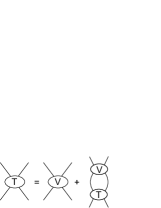
Figure 3: The Lippmann-Schwinger equation with potential $V$.

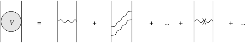
Figure 4: Some time-ordered diagrams contributing to the two-particle potential $V$ in non-relativistic QED. All orderings with at least one photon in intermediate states are included. A cross denotes energy corrections.

A remarkable feature of the discussion above is that all the photon-exchange diagrams considered scaled with negative powers of $Q$. This is rooted on our temporary restriction to diagrams built from the simplest interaction in the Lagrangian (27). It means that no new ultraviolet cutoff is needed in loop integrals, once the bare fermion charge and mass are adjusted to remove cutoff dependence in diagrams involving a single fermion. At some point in the past great importance was attributed to this “renormalizability”. Nowadays, we realize that its simple form in QED is limited. Interactions with more derivatives, which are not forbidden by symmetry and thus exist, spoil this simplification. Piling up sufficiently many higher-derivative interactions from Eq. (28), a two-fermion diagram will scale as a positive power of $Q$, and diverge in the absence of a cutoff. However, because four-fermion interactions can be constructed that are gauge invariant, the new cutoff dependence can still be eliminated by a shift in four-fermion parameters. The EFT is still renormalizable, in the sense that at any given power of $Q$ a finite number of parameters will remove cutoff dependence from observables (renormalization-group invariance). QED can be deceivingly simple because the symmetries allow couplings of dimension four, which dominate. As we are going to see next, the same does not happen in the EFT of QCD.

3 Building a QCD-based EFT

3.1 Standard model and QCD

We now focus on the energy region of interest. The EFT corresponding to the standard model at an energy scale of a few GeV involves only the lightest leptons and quarks, gluons, and the photon; weak gauge bosons, and heavy leptons and quarks can be integrated out. For simplicity, here we focus on interactions involving the lightest $u$ and $d$ quarks. They can be arranged in a flavor doublet $q=(^{u}_{d})$. The relevant pieces of the effective Lagrangian at this scale are

$${\cal L} = -\sum_{f=1}^{3}\bar{l_{f}}(\partial\!\!\!\!\!/-ieA\!\!\!\!/+m_{f})l_{f}-\frac{1}{4}F_{\mu\nu}F^{\mu\nu}$$ (38)

$$-\bar{q}(\partial\!\!\!\!\!/-ig_{s}G\!\!\!\!\!/-ieQA\!\!\!\!/)q-\frac{1}{2}(m_{u}+m_{d})\bar{q}q+\frac{1}{2}(m_{d}-m_{u})\bar{q}\tau_{3}q$$

$$-\frac{1}{2}Tr[G_{\mu\nu}G^{\mu\nu}]+\frac{\bar{\theta}g_{s}^{2}}{32\pi^{2}}\varepsilon_{\mu\nu\rho\sigma}Tr[G^{\mu\nu}G^{\rho\sigma}]+\ldots$$

Here the $l_{f}$’s are the lepton fields with mass $m_{f}$, $G_{\mu}$ ($A_{\mu}$) is the gluon (photon) field of strength $G_{\mu\nu}$ ($F_{\mu\nu}$), $\tau_{3}$ is the usual Pauli matrix, $Q=1/6+\tau_{3}/2$ is the quark charge matrix, and “$\ldots$” denote higher-dimension terms. Higher-dimension interactions are suppressed by powers of the masses of the heavy particles that have been integrated out. We will neglect them in a (very good) first approximation. We will also neglect the theta term, since the strong CP parameter $\bar{\theta}$ is found to be unnaturally small (the so-called strong CP problem). The effect of these terms can be easily incorporated in a more comprehensive analysis.

The leading Lagrangian (QCD + QED) becomes then invariant under parity and time-reversal transformations. The quark/gluon sector has 4 remaining parameters: the gauge couplings for strong ($g_{s}$) and electromagnetic ($e$) interactions, and the masses of the up ($m_{u}$) and the down ($m_{d}$) quarks.

In the chiral limit, that is, when $m_{u}=m_{d}=0$ and $e=0$, the action of the QCD Lagrangian becomes invariant under scale transformations: $x\rightarrow\lambda^{-1}x$, $q\rightarrow\lambda^{3/2}q$, and $G_{\mu}\rightarrow\lambda G_{\mu}$. Thus there is no dimensionful parameter in the Lagrangian; there is only one dimensionless parameter which is the strong-interaction coupling constant $g_{s}$. However, the scale symmetry is explicitly broken due to quantum corrections that probe high energies. A regulator is necessary, thus introducing a dimensionful parameter in the problem. As a result, $g_{s}$ becomes a “running coupling” that is a function of a momentum scale. We observe in fact that $g_{s}$ grows as the scale is lowered, and reaches $g_{s}\sim 1$ near 1 GeV. Perturbation theory in $g_{s}$, a useful tool at high energies, fails miserably at nuclear energies.

3.2 Basic assumptions about a QCD-based EFT

Thus in our pursuit to build an EFT, we have to take the properties of the nonperturbative QCD into account, even though we cannot at present deduce them. The first assumption we make is that QCD “confines”: only colorless states (hadrons) are asymptotic states. In the low-energy EFT, only hadrons need to be incorporated as fields. Our second assumption is that QCD is natural. Since almost all hadron masses $\stackrel{{\scriptstyle\textstyle>}}{{\sim}}$ $1$ GeV, we conclude that there is a characteristic QCD mass scale $M_{QCD}\sim 1$ GeV. This sets the limit of validity of the EFT.

Because we want to discuss nuclei, we certainly want to include the nucleon in the EFT. Because the delta-nucleon mass difference $\delta\equiv m_{\Delta}-m_{N}\simeq 300$ MeV $\ll M_{QCD}$, if we want to explore the full region of energies accessible to EFT, we incorporate the delta isobar as well. Nucleon and delta fields form isospin multiplets as following:

$$N=\bigl{(}\begin{smallmatrix}p\\ n\end{smallmatrix}\bigr{)} \;\;\;\;\;\;\;\;{\rm and}\;\;\;\;\;\;\;\;\;\;\;\Delta=\left(\begin{smallmatrix}\Delta^{++}\\ \Delta^{+}\\ \Delta^{0}\\ \Delta^{-}\end{smallmatrix}\right).$$ (39)

Below we denote these fermions by $\psi$. Other baryon states such as $N^{*}$ are not included, as their mass differences to the nucleon approach $M_{QCD}$ ($m_{N^{*}}-m_{N}\simeq 500$ MeV, etc.). Mesons such as the $\rho$ and the $\omega$ are not included either because they have masses ${\cal O}(M_{QCD})$. (Moreover, they interact with the pions and nucleons via dimension-four interactions that are not weak, which is at present an insurmountable obstacle for a systematic approach.)

Does the pion mass, $m_{\pi}\simeq 140$ MeV $\ll M_{QCD}$, imply a breakdown of naturalness? No! We notice that in the chiral limit the leading-order Lagrangian (38) has an $SU_{L}(2)\times SU_{R}(2)\sim SO(4)$ chiral symmetry, since it is invariant under independent $SU(2)$ rotations of left- and right-handed quarks,

$$q_{R(L)}\equiv\frac{1+(-)\gamma_{5}}{2}q\;\rightarrow\exp(i\vec{\alpha}_{R(L)}\cdot\vec{\tau})\;q_{R(L)}.$$ (40)

This symmetry is not manifest in the hadron spectrum. There is, for example, no scalar particle degenerate with the three pions. We thus make our third assumption, that chiral symmetry is spontaneously broken down to its diagonal subgroup, the $SU_{L+R}(2)\sim SO(3)$ of isospin. Although we cannot at present calculate it, the effective potential of QCD, when plotted as function of quark bilinears ($\bar{q}\mbox{${\bm{\tau}}$}i\gamma_{5}q$, $\bar{q}q$), has to have a “Mexican-hat” shape. The symmetry of the potential is $SO(4)$. The degenerate minima form thus a (four-dimensional) “chiral circle”, the radius of which we call $f_{\pi}$. (Later, we find out that $f_{\pi}$ so defined coincides with the pion decay constant.) The symmetry is broken because the world actually sits on one particular point of this circle (which is selected by the quark-mass perturbation). Excitations orthogonal to the circle should have mass $m_{\sigma}\sim M_{QCD}$, since this is the scale that sets the curvature of the effective potential. Excitations along the circle, on the other hand, are massless; the three Goldstone bosons can be associated with the light pions.

Interactions of pions in the EFT have to reproduce these symmetry properties. There are several possible parametrizations of the chiral circle which correspond to different choices of pion fields ${\bm{\pi}}$, such as the $\sigma$-model-like, the Callan-Coleman-Wess-Zumino construction, and the stereographic projection. Since a chiral transformation rotates the chiral circle, the infinitesimal transformation of the pions is $\mbox{${\bm{\pi}}$}\rightarrow\mbox{${\bm{\pi}}$}+\mbox{${\bm{\varepsilon}}$}$. The EFT Lagrangian has to have the same symmetry, which implies that the pion fields can be chosen to couple derivatively. This is very important because it means that pion interactions involve the small momentum $Q$. Moreover, because the derivative is on the chiral circle, non-linear terms

$$D^{-1}\equiv 1-\mbox{${\bm{\pi}}$}^{2}/4f_{\pi}^{2}+\ldots$$ (41)

appear. There is a well-defined procedure to construct the Lagrangian, the theory of non-linear realizations of a symmetry Callan (1969). We first define covariant objects, such as covariant derivatives that involve the associated non-linear terms: the pion covariant derivative ${\mbox{${\bm{D}}$}}_{\mu}$ and the fermion covariant derivative ${\cal D}_{\mu}$. Then, the invariant Lagrangian can be constructed as the most general $SO(3)$-invariant Lagrangian made out of covariant objects.

We can now relax the restriction to the chiral limit and consider the effect of non-vanishing quark masses. The important point is that the mass terms break $SO(4)$ in a specific way. The common-mass term is the fourth component of an $SO(4)$ vector, and the mass-difference term is the third component of another $SO(4)$ vector. The common-mass term, for example, tilts the Mexican hat in the $\bar{q}q$ direction. The chiral circle is no longer degenerate, and the pions get a common mass $m_{\pi}^{2}\sim(m_{u}+m_{d})M_{QCD}$. In the EFT, we construct all operators that break chiral symmetry in the same way. Their coefficients will be proportional to powers of $(m_{u}+m_{d})$ and $(m_{d}-m_{u})\equiv\varepsilon(m_{u}+m_{d})$.

Finally, electromagnetic interactions via “soft” photons can be added as well through all gauge-invariant terms. The one complication is that the integrating out of “hard” photons generates operators that do not necessarily involve soft photons. Such “indirect” electromagnetic operators can be constructed by looking at the chiral transformation properties of the (non-local) four-quark operators they produce. One can show that these operators break chiral symmetry as 34 and 34-34 components of $SO(4)$ antisymmetric tensors. The corresponding operators in the EFT will break isospin with strengths proportional to powers of $e^{2}$.

To sum it up, the EFT Lagrangian has two classes of interactions. One class is chiral invariant; they involve powers of the momentum and no dimension-four interactions are permissible. Another class is chiral-symmetry breaking; dimension-four operators are among the ones allowed, but they are suppressed by powers of the small quark masses or charges. As a consequence, all pion interactions are weak at low energies.

3.3 The chiral Lagrangian

Based on the above, the most general Lagrangian takes the schematic form:

$${\cal L}=\sum^{\infty}_{mnpqf} C_{mnpqf}\left(\frac{{\mbox{${\bm{D}}$}}_{\mu}}{M_{QCD}}\right)^{n}\left(\frac{{\cal D}_{\nu}}{M_{QCD}}\right)^{m}\left(\frac{{\bar{\psi}}\psi}{f_{\pi}^{2}M_{QCD}}\right)^{\frac{f}{2}}\left(\frac{\delta}{M_{QCD}}\right)^{q}\left(\frac{m_{\pi}^{2}}{M_{QCD}^{2}}\frac{\mbox{${\bm{\pi}}$}^{2}}{f_{\pi}^{2}}\right)^{p}$$ (42)

$$\times f_{\pi}^{2}M_{QCD}^{2},$$

where the $C_{mnpqf}$ are the unknown constants in the EFT. By naturalness these are of ${\cal O}(1)$ if isospin conserving and ${\cal O}(\varepsilon)$ and ${\cal O}(e^{2})$ if isospin breaking.

It is convenient to introduce the “chiral index” $\Delta$ that counts the inverse powers of the large mass scale $M_{QCD}$,

$$\Delta=n+m+q+2p+\frac{f}{2}-2\equiv d+\frac{f}{2}-2.$$ (43)

Because of chiral symmetry, there are no interactions with negative chiral index. We can then split the chiral Lagrangian in pieces ${\cal L}^{(\Delta)}$:

$$\sum_{\Delta=0}^{\infty}{\cal L}^{(\Delta)}={\cal L}^{(0)}+{\cal L}^{(1)}+{\cal L}^{(2)}+\ldots$$ (44)

The form of the Lagrangian depends on the parametrization of the pion fields. For example, using stereographic coordinates, the lower-order Lagrangians are Ordonez (1992, 1996); van Kolck (1994)

$${\cal L}^{(0)} = -2f_{\pi}^{2}\mbox{${\bm{D}}$}_{\mu}^{2}-\frac{m_{\pi}^{2}}{2}D^{-1}\mbox{${\bm{\pi}}$}^{2}+N^{\dagger}i{\cal D}_{0}N-2g_{A}\vec{\mbox{${\bm{D}}$}}\cdot N^{\dagger}\mbox{${\bm{t}}$}\vec{\sigma}N$$ (45)

$$+C_{0}^{(S)}N^{\dagger}N\;N^{\dagger}N+C_{0}^{(T)}N^{\dagger}\vec{\sigma}N\cdot N^{\dagger}\vec{\sigma}N$$

$$+\Delta^{\dagger}(i{\cal D}_{0}-\delta)\Delta-2h_{A}\vec{\mbox{${\bm{D}}$}}\cdot\left[N^{\dagger}\mbox{${\bm{T}}$}\vec{S}\Delta+h.c.\right]+\ldots,$$

$${\cal L}^{(1)} = \frac{1}{2m_{N}}N^{\dagger}\vec{\cal D}^{\,2}N-\frac{g_{A}}{2m_{N}f_{\pi}}\mbox{${\bm{D}}$}_{0}\cdot\left[iN^{\dagger}\mbox{${\bm{t}}$}\vec{\sigma}\cdot\vec{\cal D}N+h.c.\right]$$ (46)

$$-B_{1}\mbox{${\bm{D}}$}_{\mu}^{2}N^{\dagger}N-B_{2}(\vec{\mbox{${\bm{D}}$}}\times\vec{\mbox{${\bm{D}}$}})\cdot N^{\dagger}\mbox{${\bm{t}}$}\vec{\sigma}N-\frac{B_{3}m_{\pi}^{2}}{4f_{\pi}^{2}}D^{-1}\mbox{${\bm{\pi}}$}^{2}N^{\dagger}N-B_{4}\mbox{${\bm{D}}$}_{0}^{2}N^{\dagger}N$$

$$-D_{1}\vec{\mbox{${\bm{D}}$}}\cdot N^{\dagger}\mbox{${\bm{t}}$}\vec{\sigma}N\;N^{\dagger}N-D_{2}\vec{\mbox{${\bm{D}}$}}\cdot\left(N^{\dagger}\mbox{${\bm{t}}$}\vec{\sigma}N\times N^{\dagger}\mbox{${\bm{t}}$}\vec{\sigma}N\right)$$

$$-\frac{E_{1}}{2}N^{\dagger}N\;N^{\dagger}\mbox{${\bm{t}}$}N\cdot N^{\dagger}\mbox{${\bm{t}}$}N-\frac{E_{2}}{2}N^{\dagger}N\;N^{\dagger}\mbox{${\bm{t}}$}\vec{\sigma}N\cdot N^{\dagger}\mbox{${\bm{t}}$}\vec{\sigma}N$$

$$-\frac{E_{3}}{2}N^{\dagger}\mbox{${\bm{t}}$}\vec{\sigma}N\cdot\left(N^{\dagger}\mbox{${\bm{t}}$}\vec{\sigma}N\times N^{\dagger}\mbox{${\bm{t}}$}\vec{\sigma}N\right)$$

$$+\frac{1}{2m_{N}}\Delta^{\dagger}\vec{\cal D}^{\,2}\Delta-\frac{h_{A}}{2m_{N}f_{\pi}}\mbox{${\bm{D}}$}_{0}\cdot\left[iN^{\dagger}\mbox{${\bm{T}}$}\vec{S}\cdot\vec{\cal D}\Delta+h.c.\right]+\ldots$$

Here $g_{A}$, $h_{A}={\cal O}(1)$ and $B_{i}={\cal O}(1/M_{QCD})$ are undetermined constants, to be obtained either by solving QCD or by fitting data; “…” stand for other terms involving the delta isobar. Higher-index interactions can be constructed similarly.

3.4 Why is nuclear physics so interesting?

Processes that involve at most one nucleon ($A\leq 1$) can be easily described in the EFT. If all external momenta are of the same order $Q\sim M_{nuc}$, there are only two scales $Q$ and $M_{QCD}$. A generic contribution to an amplitude can be written as

$$T\sim{\cal N}\left(\frac{Q}{M_{QCD}}\right)^{\nu}{\cal F}\left(\frac{Q}{m_{\pi}}\right),$$ (47)

where ${\cal F}$ is a dimensionless non-analytic function and ${\cal N}$ is a normalization factor. Counting powers of $Q$ in a particular diagram can be done as for the superficial degree of divergence. For a diagram with $L$ loops and $V_{\Delta}$ vertices of index $\Delta$ we find Weinberg (1979)

$$\nu=2-A+2L+{\sum_{\Delta}}{V_{\Delta}}{\Delta}.$$ (48)

This formula is important because chiral symmetry places a lower bound on the interaction index ${\Delta}\geq 0$. Since $L$ is bounded from below ($L\geq 0$), $\nu\geq\nu_{min}=2-A$ for strong interactions. An expansion in $Q/M_{QCD}$ results. It starts at $\nu=\nu_{min}$ with tree ($L=0$) diagrams built out of vertices of index 0 ($\sum V_{\Delta}\Delta=0$), then proceeds at $\nu=\nu_{min}+1$ with further tree diagrams, now with one vertex of index 1, the remaining having index 0 ($\sum V_{\Delta}\Delta=1$). These first two orders are equivalent to the current algebra of the 1960’s, but now unitarity corrections can be accounted for systematically. At $\nu=\nu_{min}+2$, for example, besides tree diagrams with one index-2 interaction or two index-1 interactions ($\sum V_{\Delta}\Delta=2$), there are also one-loop ($L=1$) diagrams built out of index-0 vertices ($\sum V_{\Delta}\Delta=0$). This is generalized to higher orders in obvious fashion. An estimate of the expansion parameter is $\sim m_{\pi}/m_{\rho}\approx 0.2$. In this context the EFT is called Chiral Perturbation Theory (ChPT). See Ref. Bernard (1995) for a review.

Processes with two or more nucleons ($A\geq 2$) are much more interesting. One can see this by studying the simplest Feynman diagrams contributing to the $NN$ amplitude $T_{NN}$, shown in Fig. 5. The first diagram results in the term:

$$T_{NN}^{(1)}=\frac{g_{A}^{2}}{f_{\pi}^{2}}\frac{\vec{\sigma}_{1}\cdot\vec{q}\vec{\sigma}_{2}\cdot\vec{q}}{q^{2}+m_{\pi}^{2}}\sim\frac{g_{A}^{2}}{f_{\pi}^{2}}.$$ (49)

This is analogous to Coulomb-photon exchange in QED. By following the same steps as in that example, we see that the crossed-box diagram is

$$T_{NN}^{(2)(\times)}\sim\frac{g_{A}^{4}}{f_{\pi}^{4}}\Big{(}\frac{Q^{3}}{4\pi}\Big{)}\Big{(}\frac{1}{Q}\Big{)}\Big{(}\frac{1}{Q}\Big{)}\Big{(}\frac{Q^{2}}{Q^{2}}\Big{)}\Big{(}\frac{Q^{2}}{Q}\Big{)}\sim\frac{g_{A}^{2}Q^{2}}{4\pi f_{\pi}^{2}}\frac{g_{A}^{2}}{f_{\pi}^{2}},$$ (50)

which is small, given that $4\pi f_{\pi}\sim M_{QCD}$.

Figure 5: Simplest pion-exchange diagrams in the $NN$ amplitude.

However, the box diagram is

$$T_{NN}^{(2)(x)}\sim\frac{g_{A}^{4}}{f_{\pi}^{4}}\Big{(}\frac{Q^{3}}{4\pi}\Big{)}\Big{(}\frac{m_{N}}{Q^{2}}\Big{)}\Big{(}\frac{Q^{2}}{Q^{2}}\Big{)}\Big{(}\frac{Q^{2}}{Q^{2}}\Big{)}+\ldots\sim\frac{g_{A}^{2}m_{N}Q}{4\pi f_{\pi}^{2}}\frac{g_{A}^{2}}{f_{\pi}^{2}}+\ldots$$ (51)

The scale that sets the relative size of this diagram is not $M_{QCD}$ but

$$M_{NN}\equiv\frac{4\pi f_{\pi}^{2}}{g_{A}^{2}m_{N}},$$ (52)

which numerically is $\sim f_{\pi}\sim M_{nuc}\ll M_{QCD}$.

As in the QED case, the infrared enhancement of $m_{N}/Q$ over irreducible states appears in all reducible intermediate states. Contrary to ordinary ChPT, we need to resum the leading terms; in a schematic way,

$$T_{NN} \sim \frac{g_{A}^{2}}{f_{\pi}^{2}}\left[1+{\cal O}\left(\frac{Q}{M_{NN}}\right)+\cdots+{\cal O}\left(\frac{Q}{M_{QCD}}\right)\right]$$ (53)

$$\sim \frac{g_{A}^{2}}{f_{\pi}^{2}}\left[\frac{1}{1-{\cal O}\left(\frac{Q}{M_{NN}}\right)}+\cdots+{\cal O}\left(\frac{Q}{M_{QCD}}\right)\right].$$

Nuclear bound states thus appear at

$$Q\sim M_{NN},$$ (54)

with binding energy

$$B\sim\frac{Q^{2}}{m_{N}}\sim\frac{M_{NN}^{2}}{m_{N}}.$$ (55)

Numerically this is $\sim M_{QCD}/(4\pi)^{2}\approx 10$ MeV, which explains why nuclei are so shallow when compared to the characteristic QCD scale.

3.5 Deriving a potential for nuclear physics

We can now carry out systematic calculations by finding a power counting for the potential, defined as the sum of all irreducible diagrams, and then solving the Lippman-Schwinger equation (Fig. 3) order by order.

Weinberg Weinberg (1990) was the first to suggest a simple power counting. He reasoned that, because the enhanced states are by construction removed from the potential, powers of $Q$ could be counted in the potential as in ChPT. This results in an expansion of the form:

$$V=\sum_{\nu=0}^{\infty}c_{\nu}Q^{\nu},$$ (56)

where

$$\nu=4-A+2(L-C)+\sum_{\Delta}V_{\Delta}\Delta.$$ (57)

The only difference compared to Eq. (48) is the number of separately connected pieces $C\geq 1$. They arise because the potential is just part of the full amplitude and does not need to be fully connected.

According to this power counting, in leading order we have, besides one-pion exchange (OPE) between two nucleons, also non-derivative two-nucleon contact interactions (the $C_{0}^{(S)}$ and $C_{0}^{(T)}$ terms in Eq. (45).) A calculation of all (isospin-conserving) contributions to the two-nucleon potential up to $\nu=\nu_{min}+3$ was carried out in Refs. Ordonez (1992, 1996) using time-ordered perturbation theory. Some diagrams are shown in Fig. 6. To this order, the potential has all the spin-isospin structure of the phenomenological models, but its profile is determined by explicit degrees of freedom, symmetries, and power counting. The power counting suggests a hierarchy of short-range effects: $S$ waves should depend strongly on the short-range parameters $C_{0}^{(S,T)}$; contact interactions affect $P$-wave phase shifts only in subleading order, so their effect should be smaller and approximately linear; $D$ waves are affected by contact interactions only via mixing, while higher waves should be essentially determined by pion exchange. Chiral symmetry is particularly influential in the two-pion exchange (TPE) piece. The latter includes a particular form of terms previously considered Brueckner (1953), plus a few new terms. Those terms involving the $B_{i}$’s and the deltas provide the only form of correlated TPE to this order, as graphs where pions interact in flight appear only in next order and should thus be relatively small. The sum of the $B_{1}$ term and the corresponding delta term (related to the nucleon axial polarizability), is particularly important in providing an isoscalar central force. Not surprisingly, in the chiral limit these potentials behave at large separations as van der Waals forces. Isospin-violating pieces of the potential can be calculated as well van Kolck (1995).

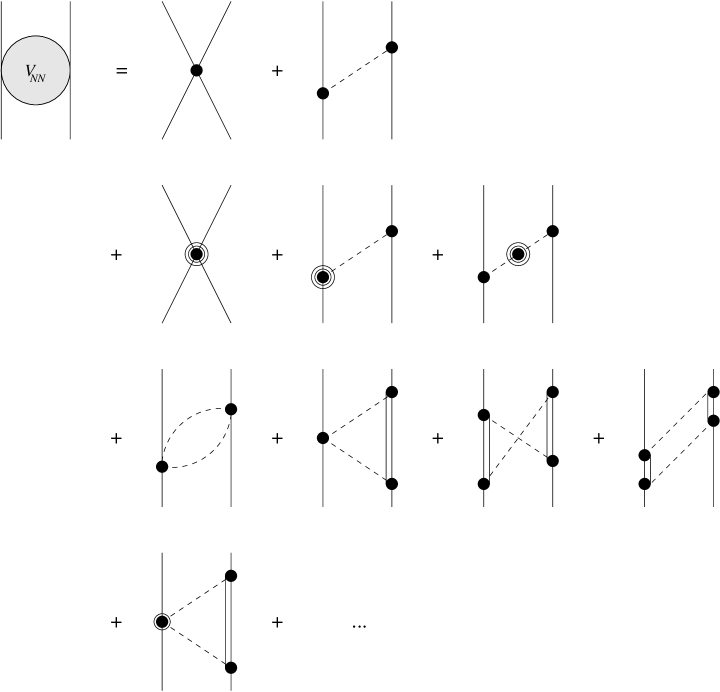
Figure 6: Some time-ordered diagrams contributing to the two-nucleon potential $V_{NN}$ in the EFT. (Double) solid lines represent nucleons (and/or deltas), dashed lines pions, a heavy dot an interaction in ${\cal L}^{(0)}$, a dot within a circle an interaction in ${\cal L}^{(1)}$, and a dot within two circles an interaction in ${\cal L}^{(2)}$. First line corresponds to $\nu=\nu_{min}$, second and third lines to $\nu=\nu_{min}+2$, fourth line to $\nu=\nu_{min}+3$, and “$\ldots$” denote $\nu\geq\nu_{min}+4$. All orderings with at least one pion or delta in intermediate states are included. Not shown are diagrams contributing only to renormalization of parameters.

Using this potential, one can then solve the Schrödinger equation. For each cutoff the parameters are fitted to data at selected energies. A sample of the results Ordonez (1996) for the lowest, most important partial waves is presented in Fig. 7, together with phases from the Nijmegen phase-shift analysis Stoks (1993). Quality of the fits is typical of other waves. Waves higher than $F$-waves were found to be mostly described well by pion exchange alone, as expected. Deuteron quantities are shown in Table 1. Electromagnetic quantities refer to the contributions from lowest-order $\gamma NN$ couplings only, not to a consistent calculation which would include sub-leading one- and two-nucleon effects. The predicted $S$-wave scattering lengths (not used to constrain the fit) were found to be $a_{2}^{(^{1}S_{0})}\simeq-15.0$ fm and $a_{2}^{(^{3}S_{1})}\simeq 5.46$ fm. Important central attraction comes from the $B_{i}$’s and deltas, and indeed the central potential does resemble those from models that include $\sigma$ and $\omega$ meson exchange explicitly Kaiser (1997) (see Fig. 8). Thus the properties of the mesons extracted from phenomenological models have limited meaning. Values for the parameters are listed in Ref. Ordonez (1996). Reasonable values were found for quantities known at the time, for example $g_{A}=1.33$ (in agreement with the Goldberger-Treiman relation) and $h_{A}=2.03$ (smaller but not too far off the large-${\cal N}_{c}$ value). However, the values for the $B_{i}$’s came out somewhat different than those found later in $\pi N$ scattering. For a cutoff of $\Lambda=780$ MeV, the coefficients $C_{2n}$ of the contact interactions were found to scale approximately with $M_{QCD}\sim 500$ MeV.

Figure 7: ${}^{1}S_{0}$, ${}^{3}S_{1}$, and ${}^{3}D_{1}$ $NN$ phase shifts and $\varepsilon_{1}$ mixing angle in degrees as functions of the laboratory energy in MeV: EFT up to $\nu=3$ for cutoffs of 500 (dotted), 780 (dashed), and 1000 MeV (solid line); and Nijmegen PSA (squares).

Table 1: Results from EFT fits at $\nu=3$ for various cut-offs $\Lambda$ and experimental values for the deuteron binding energy ($B$), magnetic dipole moment ($\mu_{d}$), electric quadrupole moment ($Q_{E}$), asymptotic $D/S$ ratio ($\eta$), and $D$-state probability ($P_{D}$).

Deuteron	$\Lambda$ (MeV)
quantities	500	780	1000	Experiment
$B$ (MeV)	2.15	2.24	2.18	2.224579(9)
$\mu_{d}$ ($\mu_{N}$)	0.863	0.863	0.866	0.857406(1)
$Q_{E}$ (fm2)	0.246	0.249	0.237	0.2859(3)
$\eta$	0.0229	0.0244	0.0230	0.0271(4)
$P_{D}$ (%)	2.98	2.86	2.40

Figure 8: The isoscalar central potential generated by two-pion exchange compared with phenomenological $\sigma+\omega$ contributions Kaiser (1997).

The EFT also offers some insight into few-nucleon forces. Weinberg’s power counting embodied in Eq. (57) suggests a hierarchy of few-nucleon forces. In leading order ($\nu=\nu_{min}=6-3A$), $C$ is maximum, so we have only pairwise interactions via the leading two-nucleon potential. We can easily verify that, if the delta is kept as an explicit degree of freedom, a $3N$ potential will arise at $\nu=\nu_{min}+2$, a $4N$ potential at $\nu=\nu_{min}+4$, and so on. It is (approximate) chiral symmetry therefore that implies that $n$-nucleon forces $V_{nN}$ obey a hierarchy of the type

$$\frac{\langle V_{(n+1)N}\rangle}{\langle V_{nN}\rangle}\sim{\cal O}\left(\frac{Q}{M_{QCD}}\right)^{2},$$ (58)

with $\langle V_{nN}\rangle$ denoting the contribution per $n$-plet. If $|\langle V_{2N}\rangle|\sim M_{QCD}/(4\pi)^{2}\approx 10$ MeV, we can expect $|\langle V_{3N}\rangle|\sim 0.5$ MeV, $|\langle V_{4N}\rangle|\sim 0.02$ MeV, and so on. This is in accord with detailed few-nucleon phenomenology based on potentials that include small $3N$ and no $4N$ forces. This is shown in Table 2 in the case of the AV18/IL2 potential Pieper (2001).

Table 2: Contributions of the two-, three- and four-nucleon potentials (per doublet, per triplet, and per quadruplet, respectively): Weinberg power counting (W pc) and calculations with the AV18/IL2 potential for the ground states of various light nuclei (²H, ³H, etc.).

(MeV)	W pc	2H	3H	4He	6He	7Li	8Be	9Be	10B
$|\langle V_{2N}\rangle|$	$\sim 10$	22	20	23	13	11	11	9.4	8.9
$|\langle V_{3N}\rangle|$	$\sim 0.5$	–	1.5	2.1	0.55	0.43	0.38	0.29	0.30
$|\langle V_{4N}\rangle|$	$\sim 0.02$	–	–	?	?	?	?	?	?
$|\langle V_{3N}\rangle|/|\langle V_{2N}\rangle|$	$\sim 0.05$	–	0.075	0.091	0.042	0.039	0.035	0.031	0.034
$|\langle V_{4N}\rangle|/|\langle V_{3N}\rangle|$	$\sim 0.05$	–	–	?	?	?	?	?	?

The new forces that appear in systems with more than two nucleons have been derived in Refs. Ordonez (1992); van Kolck (1994). The relevant terms up to $\nu_{min}+3$ are shown in Fig. 9. The leading $3N$ potential has components with three different ranges: TPE; OPE/short; and purely short. The TPE part of the potential is determined in terms of $\pi N$ scattering observables, and is similar to existing two-pion-exchange $3N$ potentials Friar (1999). The novel OPE/short-range components involve $\pi(N^{\dagger}N)^{2}$ interactions of strengths that are not fixed by chiral symmetry alone but can be determined from reactions involving only two nucleons, such as $NN\rightarrow NN\pi$ Hueber (2001). The purely short-range components of the potential can only be determined from few-nucleon systems.

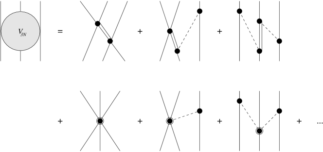
Figure 9: Some time-ordered diagrams contributing to the $3N$ potential in the pionful EFT. (Double) solid lines represent nucleons (and/or deltas), dashed lines pions, a heavy dot an interaction in ${\cal L}^{(0)}$, and a dot within a circle an interaction in ${\cal L}^{(1)}$. First line corresponds to $\nu=\nu_{min}+2$, second line to $\nu=\nu_{min}+3$, and “$\ldots$” denote $\nu\geq\nu_{min}+4$. All nucleon permutations and orderings with at least one pion or delta in intermediate states are included.

The nuclear potential from EFT has been further elaborated in the last couple of years. Calculations are being pushed to next order Kaiser (2000), better fits (with more extensive input from $\pi N$ scattering) to $NN$ data have been achieved Epelbaum (2000), and the first results for $3N$ and $4N$ systems have appeared Epelbaum (2001). These developments are all reviewed in Ref. Bedaque (2002).

Weinberg’s power counting thus provides a rationale to understand much of the phenomenology of light nuclei. At low energies, the nucleon can be visualized as in Fig. 10: the light pion states form a sparse outer cloud, leading to a loop expansion in $Q/4\pi F_{\pi}$, while the high-energy states form a dense inner cloud, amenable to a multipole expansion in terms of $Q/m_{\rho}$. Since most of the time there is only a single pion “in the air”, in the nucleus the interaction among nucleons is mostly pairwise, resulting also in a cluster expansion for the potential.

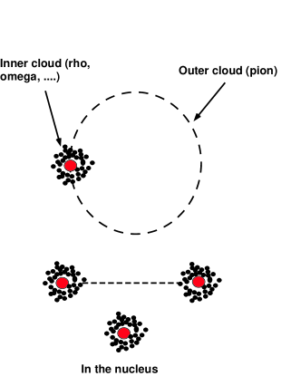
Figure 10: The short-ranged ($\rho$, etc.) cloud around the nucleon and the long-ranged ($\pi$) cloud surrounding it.

3.6 Renormalization

Despite all similarities, there is an important difference between the nuclear and atomic potentials. Because of chiral symmetry, the potential from one-pion exchange goes as $Q^{0}$, from two-pion exchange as $Q^{2}$, and so on. The loops generated by the iteration of these potentials are then sensitive to the cutoff. In coordinate-space parlance, these potentials are singular, that is, they behave for small radial distances $r$ as $1/r^{3}$, $1/r^{5}$, and so on. The Schrödinger equation for such potentials is not well defined. Clearly, one cannot consider pion exchange without including enough short-distance operators to erase the cutoff dependence from observables.

Now, Weinberg’s power counting automatically predicts which contact operators have to be taken at each order. Following this prescription, it does seem that the fits are of the same quality for different cutoffs. However, the numerical character of the calculations makes it hard to offer a proof of consistency. It is not apparent, for example, how a momentum-independent short-range interaction can renormalize the OPE potential (49).

Much effort has been devoted to this issue in the last five years Bedaque (2002). A search for more analytical approaches led to extensive studies of the EFT at momenta $Q\ll m_{\pi}$. In this regime, pions can be treated as heavy particles. All interactions are of contact type, and form an expansion in $Q/M_{nuc}$. This “pionless” EFT can be solved by hand in the $NN$ sector, and by very simple numerical means in the $3N$ and $4N$ systems. Power counting and renormalization are not without surprises, but they can be done consistently. Of course, the pionless EFT does not address the problem of pion exchange directly, but it goes a long way in elucidating how EFTs work in a non-perturbative context. Moreover, it is useful for many low-energy reactions, to which it has by now been applied.

As $Q$ is increased, the approximation of zero-range propagation for pions becomes less and less reliable. At momenta $Q\sim m_{\pi}$, pions have to be included explicitly in the theory. Once pions have been reinstated, we can still consider the low-$Q$ region. Because of chiral symmetry, it is reasonable to suppose that pion interactions are perturbative at sufficiently low $Q$. Based on the power counting of the pionless EFT, a new power counting was formulated that led to a manifestly consistent EFT where pion exchange was treated in perturbation theory Kaplan (1998). Unfortunately, it has been shown that the range of validity of this power counting is $Q$ $\stackrel{{\scriptstyle\textstyle<}}{{\sim}}$ $100$ MeV Fleming (2000). In this region the simplest pionless EFT is more useful.

Recently, the non-perturbative renormalization of pion exchange was analyzed Beane (2002). It was found that OPE can be renormalized à la Weinberg, provided one expands in the pion mass even the pion propagators. If one does not do expand, one makes numerically small but conceptually large errors. The full implication of this conclusion to previous results remains to be explored.

3.7 Nuclear matter on a lattice

The nuclear EFT that has been sketched above can be used to study nuclear matter at finite temperature. This provides a link with RHIC physics that is the subject of this meeting.

The general concept of a nuclear matter calculation consists of nucleons interacting via a variety of components of the nuclear potential. While the ultimate goal is to use EFT interactions, let us concentrate for simplicity on few parts of the $NN$ potential, namely central, spin- and isospin-exchange. The Hamiltonian,

$$\hat{\cal H}=\hat{\cal K}+\hat{\cal V},$$ (59)

can be expressed in second quantization and contains kinetic and potential operators. The kinetic term is written as

$$\hat{\cal K}=-\psi^{\dagger}\frac{\nabla^{2}}{2m_{N}}\psi,$$ (60)

while the potential is taken as

$$\hat{\cal V}=C_{0}\left(\psi^{\dagger}\psi\right)^{2}+C_{2}\left(\psi^{\dagger}\nabla\psi\right)^{2}.$$ (61)

The fermion operator $\psi^{\dagger}$ creates a nucleon of spin and isospin $(\sigma,\tau)$ at location $\vec{x}$, while its adjoint $\psi$ destroys it. This Hamiltonian describes merely a toy model for developing the formalism. More complicated Hamiltonians arising from full-fledged nuclear EFT can be later used for more realistic calculations.

How can we deal with the complication of many nucleons? A natural approach, patterned after similar attempts in QCD, is to investigate nuclear matter on a three-dimensional cubic lattice of spacing $a$ and periodic boundary conditions. We describe the nuclear-matter Monte Carlo method Mueller (2000), which consists of the thermal formalism to express the grand-canonical partition function as an integral over single-body evolution operators. At its center stands the Hubbard-Stratonovitch transformation, which is used to reduce the many-body problem to an effective one-body problem.

In order to study thermal properties of nuclear matter, the grand-canonical partition function at a given temperature $T=\beta^{-1}$ needs to be determined:

$$Z={\rm\hat{Tr}}\left[\exp\left(-\beta\left(\hat{\cal H}-\psi^{\dagger}\mu\psi\right)\right)\right]\equiv{\rm\hat{Tr}}\left[\hat{U}\right],$$ (62)

with $\mu$ as the chemical potential. $\hat{U}$ is called the imaginary-time evolution operator of the system and is a many-body operator; the trace is taken over all many-body states. The partition function $Z$ is an exponential over all one- and two-body operators (and therefore interactions) present in the system. It is impossible to deal with $Z$ in this form, because the number of many-body correlations that have to be kept track of grows rapidly with system size. We therefore find an expression for $Z$ that is based on a single-particle representation, replacing the many-body problem with that of non-interacting nucleons that are coupled to a heat bath of auxiliary fields. A thermal observable $\langle\hat{O}\rangle$ is then expressed as Loh (1992)

$$\langle\hat{O}\rangle=\frac{1}{Z}{\rm\hat{Tr}}\left[\hat{O}\exp\left(-\beta\left(\hat{{\cal H}}-\psi^{\dagger}\mu\psi\right)\right)\right]=\frac{\int{\cal D}[\chi]G(\chi)\langle\hat{O}(\chi)\rangle\xi(\chi)}{\int{\cal D}[\chi]G(\chi)\xi(\chi)},$$ (63)

where the Gaussian factor $G$ is given by

$$G\left(\chi\right)=\prod_{m=1}^{n_{t}}\prod_{\vec{x}_{n}}\prod_{i}\exp\left(-|\alpha_{i}|\chi^{2}_{m,\vec{x}_{n},i}\right).$$ (64)

The integrals in this equation can then be evaluated using the Metropolis algorithm Metropolis (1953) (Monte Carlo simulations).

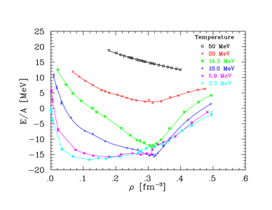
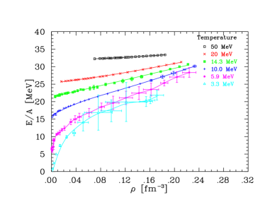
Figure 11: $E/A$ for symmetric nuclear (left) and pure neutron (right) matter as a function of density $\rho$ and for different temperatures. The purpose of the lines is to guide the eye.

Fig. 11 Mueller (2000) shows that such calculations are feasible. It displays the energy per particle $E/A$ for symmetric nuclear matter and for pure neutron matter as a function of density $\rho$ and for different temperatures. The two interaction parameters were adjusted so that the known qualitative features of the symmetric nuclear matter are reproduced. With decreasing temperature, symmetric nuclear matter develops a minimum at $\rho=0.32\;{\rm fm^{-3}}$ first, which is most pronounced between $10-14\;{\rm MeV}$, before it shifts to lower densities. At $T=3.3\;{\rm MeV}$ and $T=5.9\;{\rm MeV}$ the minimum is very broad, making matter softer. For high temperatures and/or high density, the simulation suffers from the fact that it runs out of model space. At $T=50\;{\rm MeV}$ the system behaves almost like a Fermi gas and the energy per particle should behave like $\sim\rho^{2/3}$. Yet, the curve bends down. Also, for all other temperatures, the curves converge to the energy of the full lattice state, $E/A=5.96\;{\rm MeV}$, as density increases. For sub-saturation densities the model gives more binding if compared to other calculations (see, for example, Ref. Wiringa (1988)), and the energy is not as high for densities beyond saturation. At $\rho=0.32\;{\rm fm^{-3}}$, $E/A$ as a function of temperature has a minimum at $T\approx 10\;{\rm MeV}$ which means that at even lower temperatures $E/A$ increases again. We see some evidence for a liquid-gas phase transition. The uncertainties for pure neutron matter are much larger than for symmetrical nuclear matter. As a potential, we used the parameters obtained from the fit to symmetric nuclear matter, even though we could have fitted the potential parameters for this case anew. Therefore we view the results for pure neutron matter more as a test to see how well the given potential already reproduces the energy. Note that the slopes of the curves at high temperatures are not negative as they are for symmetric nuclear matter. But clearly, we cannot conclude that the energies at $T=3.3\;{\rm MeV}$ have converged to that of the ground state because the curve differs quite a bit from that of $T=5.9\;{\rm MeV}$. At the lowest temperature they are $4-5\;{\rm MeV}$ higher than those of the ground state as calculated in Ref. Wiringa (1988), but the general shape of the curve is very similar. This is no surprise, since pure neutron matter is like a Fermi gas, with attractive forces between neutrons lowering the energies with respect to the non-interacting system. The search for any kind of phase transition in the range of $5-50\;{\rm MeV}$ was to no avail.

4 Conclusion

We have presented an introduction to EFT and some of the mileposts along the sinuous road from QCD to nuclear physics. We discussed some of the essential features of the interactions among nucleons and some of their consequences to few-nucleon systems. We can already see how to approach the solution of the important problem of finite-temperature nuclear matter. Yet, there is no denying that much is still to be done in straightening the path already traveled, and in breaking new ground. It is a good time to be on the road!

References

- Bedaque (2002) Bedaque, P.F., and van Kolck, U., nucl-th/0203055, to appear in Ann. Rev. Nucl. Part. Sci.; van Kolck, U., Nucl. Phys. A699, 33 (2002).
- Phillips (2001) Phillips, D., nucl-th/0203040, to appear in Czech. J. Phys.
- Gerber (1989) Gerber, P., and Leutwyler, H., Nucl. Phys. B321, 387 (1989).
- Rafelski (1980) Hagedorn, R., and Rafelski, J., Phys. Lett. B97, 136 (1980).
- Karsch (2000) Karsch, F., AIP Conf. Proc. 602, 323 (2001).
- Braaten (1999) Braaten, E., and Nieto, A., Eur. Phys. J. B11, 143 (1999); Hammer, H.-W., and Furnstahl, R.J., Nucl. Phys. A678, 277 (2000).
- Weinberg (1979) Weinberg, S., Physica A96, 327 (1979).
- Ball (1994) Ball, R.D., and Thorne, R.S., Ann. Phys. 236, 117 (1994).
- Georgi (1990) Georgi, H., Phys. Lett. B240, 447 (1990).
- Callan (1969) Coleman, S., Wess, J., and Zumino, B., Phys. Rev. 177, 2239 (1969); Callan, C.G., Coleman, S., Wess, J., and Zumino, B., Phys. Rev. 177, 2247 (1969).
- Ordonez (1992) Ordóñez, C., and van Kolck, U., Phys. Lett. B291, 459 (1992).
- Ordonez (1996) Ordóñez, C., Ray, L., and van Kolck, U., Phys. Rev. C53, 2086 (1996).
- van Kolck (1994) U. van Kolck, Phys. Rev. C49, 2932 (1994).
- Bernard (1995) Bernard, V, Kaiser, N, and Meißner, U-G., Int. J. Mod. Phys. E4, 193 (1995).
- Weinberg (1990) Weinberg, S., Phys. Lett. B251, 288 (1990); Nucl. Phys. B363, 3 (1991).
- Brueckner (1953) Brueckner, K., and Watson, K., Phys. Rev. 92, 1023 (1953); Sugawara, H., and Okubo, S., Phys. Rev. 117, 605 (1960); Sugawara, H., and von Hippel, F., Phys. Rev. 172, 1764 (1968).
- Stoks (1993) Stoks, V.G.J., Klomp, R.A.M., Rentmeester, M.C.M., and de Swart, J.J., Phys. Rev. C48, 792 (1993).
- Kaiser (1997) Kaiser, N., Brockmann, R., and Weise, W., Nucl. Phys. A625, 758 (1997).
- van Kolck (1995) van Kolck, U., Few-Body Syst. Suppl. 9 444 (1995); van Kolck, U., Friar, J.L., and Goldman, T., Phys. Lett. B371, 169 (1996); van Kolck, U., Rentmeester, M.C.M., Friar, J.L., Goldman, T., and de Swart, J.J., Phys. Rev. Lett. 80, 4386 (1998); Friar, J.L., and van Kolck, U., Phys. Rev. C60, 034006 (1999); Niskanen, J.A., Phys. Rev. C65, 037001 (2002).
- Pieper (2001) Pieper, S.C., and Wiringa R.B., Ann. Rev. Nucl. Part. Sci. 51, 53 (2001).
- Friar (1999) Friar, J.L., Hüber, D., and van Kolck, U., Phys. Rev. C59, 53 (1999).
- Hueber (2001) Hüber, D., Friar, J.L., Nogga, A., Witała, H., and van Kolck, U., Few-Body Syst. 30, 95 (2001); Hanhart, C., van Kolck, U., and Miller, G.A., Phys. Rev. Lett. 85, 2905 (2000).
- Kaiser (2000) Kaiser, N., Phys. Rev. C61, 014003 (2000); C62, 024001 (2000); C63, 044010 (2001); C64, 057001 (2001); C65, 017001 (2002).
- Epelbaum (2000) Epelbaum, E., Glöckle, W., and Meißner, U.-G., Nucl. Phys. A671, 295 (2000); Entem, D.R., and Machleidt, R., Phys. Lett. B524, 93 (2002); Walzl, M., Meißner, U.-G., and Epelbaum, E., Nucl. Phys. A693, 663 (2001).
- Epelbaum (2001) Epelbaum, E., Kamada, H., Nogga, A., Witała, H., Glöckle, W., and Meißner, U.-G., Phys. Rev. Lett. 86, 4787 (2001).
- Kaplan (1998) Kaplan, D.B., Savage, M.J., and Wise, M.B., Nucl. Phys. B534, 329 (1998).
- Fleming (2000) Fleming, S., Mehen, T., and Stewart, I.W., Nucl. Phys. A677, 313 (2000).
- Beane (2002) Beane, S.R., Bedaque, P.F., Savage, M.J., and van Kolck, U., Nucl. Phys. A700, 377 (2002).
- Mueller (2000) Müller, H.-M., Koonin, S.E., Seki, R., and van Kolck, U., Phys. Rev. C61, 044320 (2000).
- Loh (1992) Loh Jr., E.Y., and Gubernatis, J., in Electronic Phase Transitions, ed. by W. Hanke and Yu.V. Kopaev Elsevier, New York, 1992; Lang, G., Johnson, C., Koonin, S., and Ormand, W., Phys. Rev. C48, 1518 (1993).
- Metropolis (1953) Metropolis, N., Rosenbluth, A., Rosenbluth, M., Teller, A., and Teller, E., J. Chem. Phys. 21, 1087 (1953).
- Wiringa (1988) Wiringa, R.B., Fiks, V., and Fabrocini, A., Phys. Rev. C38, 1010 (1988); Akmal, A., and Pandharipande, V.R., Phys. Rev. C56, 2261 (1997).