Correlations beyond the mean field in Magnesium isotopes: Angular momentum projection and configuration mixing.

Abstract

The quadrupole deformation properties of the ground and low-lying excited states of the even-even Magnesium isotopes with N ranging from 8 to 28 have been studied in the framework of the angular momentum projected generator coordinate method with the Gogny force. It is shown that the N=8 neutron magic number is preserved (in a dynamical sense) in $\@@nuc{20}{Mg}$ leading to a spherical ground state. For the magic numbers N=20 and N=28 this is not the case and prolate deformed ground states are obtained. The method yields values of the two neutron separation energies which are in much better agreement with experiment than those obtained at the mean field level. It is also obtained that $\@@nuc{40}{Mg}$ is at the neutron dripline. Concerning the results for the excitation energies of the $2^{+}$ excited states and their transition probabilities to the ground state we observe a good agreement with the available experimental data. On the theoretical side, we also present a detailed justification of the prescription used for the density dependent part of the interaction in our beyond-mean-field calculations.

, and

1 Introduction

Thanks to the new breed of Radioactive Isotope Beam (RIB) facilities set up in the last years all over the world the study of exotic systems far away from the valley of stability has become one of the main topics in today’s nuclear physics. On the neutron rich side, because neutrons do not carry electric charge, the dripline can extend far away from the valley of stability. Many neutron rich regions have been the subject of detailed studies in recent years and just to give an example one should mention the regions around the magic neutron numbers N=20 and N=28. These exotic systems show many new interesting features which deserve a careful study [1, 2, 3, 4, 5, 6, 7, 8, 9, 10]. Among them, the weakening of the neutron magic numbers N=20 and N=28 in some nuclei is probably the most challenging to study.

It was in the neutron rich region N $\approx$ 20 where the breaking of a shell closure was first detected [11] and related with a shape transition to prolate deformed shapes [12]. Ground state deformations in this region easily explain the anomalous isotope shift observed in $\@@nuc{31}{Na}$ [13] as well as the decrease in the two neutron separation energy $S_{2N}$ in $\@@nuc{31,33,35}{Na}$ and $\@@nuc{30}{Ne}$ [11, 13]. A large deformation has also been inferred in the N=20 nucleus $\@@nuc{32}{Mg}$ through the measurements of $B(E2,0_{1}^{+}\rightarrow 2_{1}^{+})$ transition probabilities [14]. In addition, the low excitation energy of the first $2_{1}^{+}$ excited state [15, 16] in $\@@nuc{32}{Mg}$ and the ratio $E(4^{+})/E(2^{+})=2.6$ are consistent with the expectations for a rotational state. Recently, evidence for a rotational band in $\@@nuc{31}{Na}$ has also been obtained [17]. Although indirect, another evidence for the deformed nature of the $\@@nuc{32}{Mg}$ ground state comes from the strong ground state deformation of $\@@nuc{34}{Mg}$ inferred from the large value of the $B(E2,0_{1}^{+}\rightarrow 2_{1}^{+})$ transition probability measured [18] in this nucleus and the $E(4^{+})/E(2^{+})$ ratio of 3.18 [19, 20] which is very close to the rotational limit. Further evidence for deformed ground states in the neutron rich Mg isotopes have also been obtained experimentally [21, 22, 23]. In addition, the quadrupole collectivity in $\@@nuc{32-38}{Si}$ was experimentally studied in [24]. Finally, an extensive account of older experimental results can be found in Refs. [25, 26].

In the framework of the mean field approximation the $\@@nuc{32}{Mg}$ ground state has been found to be spherical (see for example [27, 28, 29, 30, 31, 32]) but it has also been argued that dynamical correlations may play an important role in this and other nuclei of the region. In particular, the results presented in [12, 33, 34, 35, 36, 37, 38, 39] gave initial hints concerning the importance of the restoration of symmetries and configuration mixing in some of the exotic nuclei considered. From the Shell Model point of view, the large deformations around N=20 have been explained by invoking excitations of pairs of neutrons across the N=20 shell gap (2 $\hbar\omega$ configurations). In a small set of nuclei (the island of inversion) the coexisting 2 $\hbar\omega$ intruder states actually fall below the normal 0 $\hbar\omega$ states and become the ground state configurations. In this way Shell Model calculations with different levels of complexity [40, 41, 42, 43, 44, 45, 46] have been able to explain the increased quadrupole collectivity around N=20.

The existence of anomalies in shell closures, as already found in nuclei with N $\approx$ 20, is one of the main features for the experimental and theoretical studies carried out up to now in the neutron rich nuclei with N$\approx$ 28. The $\beta$-unstable nuclei around $\@@nuc{44}{S}$ have attracted particular interest since these nuclei play an important role in the nucleosynthesis process. The experimental study of the $\beta$-decay properties of $\@@nuc{44}{S}$ (N=28) indicated [47, 48] that this nucleus is deformed. This has been confirmed in subsequent intermediate energy Coulomb excitation studies [49, 50, 51]. More recent experiments on nuclei of this region [52, 53] suggest that $\@@nuc{44}{S}$ is indeed a deformed nucleus but with strong shape coexistence making more challenging its theoretical description.

The region N $\approx$ 28 has been studied using the Skyrme Hartree-Fock (HF) model and the relativistic mean field approximation (RMF) [54, 55, 56, 57, 58]. These studies also showed the onset of deformation for some nuclei with N $\approx$ 28. Surprisingly, in none of these mean field calculations the rotational energy correction has been considered in spite that it is known to be a key ingredient for a proper description of the energy landscape as a function of the quadrupole deformation. However, in the mean field calculations of [34] with several parameterizations of the Skyrme interaction, in the calculation reported in [38] in the framework of the Bohr Hamiltonian method with the Gogny interaction or in our recent study [59] of the phenomenology of quadrupole collectivity around N=28 the rotational energy correction was explicitly taken into account either in an approximate way or exactly. The conclusions extracted from those calculations concerning the erosion of the shell closure at N=28 do not differ qualitatively (but they do in the quantitative side) from the ones extracted from the calculations without the rotational energy correction. This indicates that the N=28 shell closure can be more easily broken than the N=20 one (see also [60]). From the Shell Model point of view an erosion of the N=28 shell closure in the sulphur isotopes has also been found in calculations with the full $sd$ shell for protons and the full $pf$ shell for neutrons (see, for example [61]).

The purpose of this paper is to perform a systematic study, in the nuclei $\@@nuc{20-40}{Mg}$, of the quadrupole deformation properties of the ground and excited states. This isotopic chain contains the three spherical magic numbers N=8, N=20 and N=28 and therefore it is a good testing ground to examine both the systematic of deformation and the possible erosion of spherical shell closures. Besides, most of the considered nuclei are examples where the mean field energy landscape as a function of quadrupole deformation shows prolate and oblate minima which are practically degenerate in energy. Therefore, the correlation energies associated with the restoration of broken symmetries (mainly the rotational symmetry) and the collective quadrupole motion have to be considered at the same time. In the present study both effects are taken into account in the framework of the Angular Momentum Projected Generator Coordinate Method [37, 39, 59, 62]. The main reason to perform an exact angular momentum projection is that the usual approximations, like the Gaussian Overlap Approximation (GOA), used to compute the rotational energy correction as well as the $B(E2)$ transition probabilities are not expected to work well [36, 63] at least for some of the nuclei considered in this study.

We have used in our calculations the Gogny interaction [64] with the parameterization $D1S$ [65]. The use of the Gogny interaction in this systematic study is justified not only by the fact that this interaction provides reasonable results for many nuclear properties all over the nuclear chart, but also by the good description of the phenomenology of quadrupole collectivity in the regions N $\approx$ 20 and N $\approx$ 28 obtained recently in the same framework as the one used in this study [36, 37, 39, 59] as well as in the context of the Bohr collective Hamiltonian [33, 38]. As the results presented in this paper will show, this force also provides reasonable results for the systematic description of the phenomenology of quadrupole collectivity in the chain of Magnesium isotopes.

The paper is organized as follows: in Section 2, we describe the theoretical formalisms used in the present paper. These formalisms are the Angular Momentum Projection (AMP) and the Angular Momentum Projected Generator Coordinate Method (AMPGCM) [36, 37, 39, 59, 62] with the axially symmetric quadrupole moment as generating coordinate. The angular momentum projection technique is presented in section 2.1 where also special attention is paid to the specific problems appearing in the case of a density dependent interaction like the Gogny force. In section 2.2 we present the simplified expressions corresponding to the results of 2.1 in the case of axially symmetric intrinsic wave functions. Configuration mixing of angular momentum projected Hartree-Fock-Bogoliubov states is presented in section 2.3. There we also present the expressions to compute both transition probabilities and spectroscopic quadrupole moments (for more details the reader is referred to Appendix A). The results of our calculations for several Magnesium isotopes are discussed in Section 3. In section 3.1 we present the results for the underlying mean field studies. In section 3.2 the topological changes introduced in the mean field potential energy surfaces due to the exact restoration of the rotational symmetry are presented and then the results of the angular momentum projected configuration mixing calculations are discussed and compared with the available experimental data and other theoretical calculations. Finally Section 4 is devoted to some concluding remarks.

2 Theoretical framework: Angular momentum projection and configuration mixing

As the results of the next sections will show, the mean field approximation is just an starting point and additional correlations have to be incorporated in order to properly describe the considered nuclei. The small energy differences observed between the coexisting minima indicate that many body effects beyond the mean field, like the restoration of the rotational symmetry and/or quadrupole fluctuations, may change the conclusions extracted from the raw Hartree-Fock-Bogoliubov approximation. The restoration of the rotational symmetry leads to an energy gain (the so called rotational energy correction) which is proportional to the quadrupole deformation of the intrinsic state and ranges from zero (spherical intrinsic state) to a few MeV for typical well deformed configurations in the region of the nuclear chart considered in this study. Therefore, the consideration of this effect might play a key role for a more qualitative and quantitative description of the nuclei we are interested here. In addition, it is very important to consider the effect of quadrupole mixing [35, 36, 37, 39, 59, 63]) in those cases where the angular momentum projected potential energy surfaces show important topological changes compared with the corresponding mean field surfaces.

The theoretical background for the restoration of rotational symmetry is treated extensively in the literature (see, for example, Refs. [66, 67, 68, 69, 70, 71]) and also very good books and papers concerning the treatment of correlations beyond mean field in the framework of the Generator Coordinate Method (GCM) are available (see, for example, Refs. [63, 66, 72]). Thus we are not going to dwell on these details here. In spite of this we believe that it is useful to present a short outlook of our procedure to carry out both angular momentum and configuration mixing in the case of a density dependent interaction like the Gogny force. In addition, the issue of which density dependence has to be used in these calculations beyond mean field will be discussed in detail and strong arguments in favor of the prescription used will be given.

2.1 Angular momentum projection with density dependent interactions.

Let us consider a set of mean field states $\mid\varphi(\vec{q})\rangle$ depending on the parameters $\vec{q}=\{q_{20},q_{22},q_{40},\dots\}$ which define the corresponding mean field configurations. From this set we can build another set of states where the rotational symmetry is restored [66, 67, 68, 69, 70, 71]

$$\mid\Psi_{IM}(\vec{q})\rangle = \sum_{K}g_{K}^{I}(\vec{q})\hat{P}_{MK}^{I}\mid\varphi(\vec{q})\rangle.$$ (1)

The operator $\hat{P}_{MK}^{I}$ is the angular momentum projection operator [73] given by

$$\hat{P}_{MK}^{I} = \frac{2I+1}{8{\pi}^{2}}\int d\Omega\mathcal{D}_{MK}^{I*}(\Omega)\hat{R}(\Omega)$$ (2)

with $\Omega$ representing the set of the three Euler angles $\left(\alpha,\beta,\gamma\right)$, $\mathcal{D}_{MK}^{I}(\Omega)$ is the well known Wigner function [74] and $\hat{R}(\Omega)=e^{-i\alpha\hat{J}_{z}}e^{-i\beta\hat{J}_{y}}e^{-i\gamma\hat{J}_{z}}$ is the rotation operator. The energy $E^{I}(\vec{q})$ is given by

$$E^{I}(\vec{q})=\frac{\langle\Psi_{IM}(\vec{q})\mid\hat{H}\mid\Psi_{IM}(\vec{q})\rangle}{\langle\Psi_{IM}(\vec{q})\mid\Psi_{IM}(\vec{q})\rangle}$$ (3)

The above procedure is based on the assumption that the hamiltonian is rotational invariant and therefore the intrinsic energy $\langle\varphi(\vec{q})|\hat{H}|\varphi(\vec{q})\rangle$ is independent of the orientation of the intrinsic wave function $|\varphi(\vec{q})\rangle$, that is

$$\langle\varphi(\vec{q})|\hat{H}|\varphi(\vec{q})\rangle=\langle\varphi(\vec{q})|\hat{R}^{\dagger}(\Omega)\hat{H}\hat{R}(\Omega)|\varphi(\vec{q})\rangle$$ (4)

However, when dealing with density dependent (DD) forces the above assumption apparently breaks down as, in general, the density dependent term is not rotational invariant. This apparent paradox can be solved if density dependent hamiltonians are thought not as genuine hamiltonians but rather as devices to get an elaborated energy functional of the density. With this point of view the right hand side of Eq. (4) has to be treated as

$$\langle\varphi(\vec{q})|\hat{R}^{\dagger}(\Omega)\hat{H}[\bar{\rho}_{\Omega,\Omega}(\vec{r})]\hat{R}(\Omega)|\varphi(\vec{q})\rangle$$ (5)

where the interaction depends on the rotated density

$$\bar{\rho}_{\Omega,\Omega}(\vec{r})=\langle\varphi(\vec{q})|\hat{R}^{\dagger}(\Omega)\hat{\rho}(\vec{r})\hat{R}(\Omega)|\varphi(\vec{q})\rangle$$ (6)

with the density operator defined in the usual way

$$\hat{\rho}(\vec{r})=\sum^{A}_{i=1}\delta(\vec{r}-\vec{r}_{i})$$ (7)

Before proving that Eq. (4) holds for density dependent interactions let us present some basic results. First, we introduce the $3\times 3$ unitary rotation matrix $\mathcal{R}(\Omega)\equiv\mathcal{R}_{z}(\alpha)\mathcal{R}_{y}(\beta)\mathcal{R}_{z}(\gamma)$ that appears when eigenstates $\mid\vec{r}\rangle$ of the position operator are rotated

$$\hat{R}(\Omega)\mid\vec{r}\rangle=\mid\mathcal{R}\vec{r}\rangle.$$ (8)

This is the same matrix that appears when vector operators (like the position operator) are rotated

$$\hat{R}^{\dagger}(\Omega)\hat{\vec{r}}\hat{R}(\Omega)=\mathcal{R}(\Omega)\hat{\vec{r}}$$ (9)

Now we have to consider the role played by the density operator. Its mean value (or overlap) appears in the density dependent part of the hamiltonian and therefore the “parameter” $\vec{r}$ of Eq. (7) has to be treated as the position operators in that case. As a consequence the action of the rotation operator on $\vec{r}$ has to be considered

$$\hat{R}^{\dagger}(\Omega)\hat{\rho}(\vec{r})\hat{R}(\Omega)=\hat{\rho}(\mathcal{R}(\Omega)\vec{r})=\sum^{A}_{i=1}\delta(\mathcal{R}(\Omega)\vec{r}-\vec{r}_{i})=\sum^{A}_{i=1}\delta(\vec{r}-\mathcal{R}^{\dagger}(\Omega)\vec{r}_{i})$$ (10)

as well as its action on the internal coordinates $\vec{r}_{i}$

$$\hat{R}^{\dagger}(\Omega)\hat{\rho}(\vec{r})\hat{R}(\Omega)=\sum^{A}_{i=1}\delta(\vec{r}-\mathcal{R}(\Omega)\vec{r}_{i})=\sum^{A}_{i=1}\delta(\mathcal{R}^{\dagger}(\Omega)\vec{r}-\vec{r}_{i})=\hat{\rho}(\mathcal{R}^{\dagger}(\Omega)\vec{r}).$$ (11)

With these results we have for the rotated density of Eq. (6) that

$$\hat{R}^{\dagger}(\Omega)\bar{\rho}_{\Omega,\Omega}(\vec{r})\hat{R}(\Omega)=\langle\varphi(\vec{q})|\hat{R}^{\dagger}(\Omega)\hat{\rho}(\mathcal{R}(\Omega)\vec{r})\hat{R}(\Omega)|\varphi(\vec{q})\rangle=\langle\varphi(\vec{q})|\hat{\rho}(\vec{r})|\varphi(\vec{q})\rangle=\rho(\vec{r})$$

The first identity is the result of applying Eq. (10) whereas the second is the result of applying Eq. (11). The result thus obtained shows that even for density dependent forces Eq. (4) holds.

In order to evaluate the projected energy we need to know the Hamiltonian overlaps $\langle\varphi\mid\hat{R}^{\dagger}(\Omega)\hat{H}\hat{R}(\Omega^{\prime})\mid\varphi\rangle$. For density independent and rotational invariant interactions the hamiltonian overlap is simply given by $\langle\varphi\mid\hat{H}\hat{R}(\Omega^{\prime}-\Omega)\mid\varphi\rangle$. For density dependent interactions this quantity is not well defined and therefore we have to look for a prescription for the density dependent term. The most popular prescription so far is to use the density

$$\overline{\rho}_{\Omega,\Omega^{\prime}}(\vec{r})=\frac{\langle\varphi(\vec{q})\mid\hat{R}^{\dagger}(\Omega)\hat{\rho}(\vec{r})\hat{R}(\Omega^{\prime})\mid\varphi(\vec{q})\rangle}{\langle\varphi(\vec{q})\mid\hat{R}^{\dagger}(\Omega)\hat{R}(\Omega^{\prime})\mid\varphi(\vec{q})\rangle}$$ (12)

in the density dependent part of the interaction. Several arguments to show the credibility of this prescription have been given. For example, for those Skyrme forces, with a linear dependence in the density, that can be cast as a three body force the hamiltonian overlap can be computed without ambiguity and the resulting density dependent term depends on the density of Eq. (12). Arguments based on the extended Wick theorem (the fundamental tool to compute the overlap of operators between different product wave functions) are also very popular. Apart from the previous arguments, it is mandatory for the prescription to be used that it fulfills the following two requirements: First, it should not carry angular momentum or, in other words, the following identity should be fulfilled

$$\langle\Psi_{I_{1}M_{1}}(\vec{q})\mid\hat{H}\mid\Psi_{I_{2}M_{2}}(\vec{q})\rangle=\delta_{I_{1}I_{2}}\delta_{M_{1}M_{2}}\langle\Psi_{I_{1}M_{1}}(\vec{q})\mid\hat{H}\mid\Psi_{I_{1}M_{1}}(\vec{q})\rangle.$$ (13)

Second, the prescription must lead to a real projected energy (notice that, in general, the density of Eq. (12) is a complex quantity).

The first requirement (Eq. (13)) is a direct consequence of the property

$$\overline{\rho}_{\Omega,\Omega^{\prime}}(\vec{r}) = \frac{\langle\varphi(\vec{q})\mid\hat{R}^{\dagger}(\Omega)\hat{\rho}(\vec{r})\hat{R}(\Omega^{\prime})\mid\varphi(\vec{q})\rangle}{\langle\varphi(\vec{q})\mid\hat{R}^{\dagger}(\Omega)\hat{R}(\Omega^{\prime})\mid\varphi(\vec{q})\rangle}$$

$$= \frac{\langle\varphi(\vec{q})\mid\hat{\rho}(\mathcal{R}^{\dagger}(\Omega)\vec{r})\hat{R}(\Omega^{\prime}-\Omega)\mid\varphi(\vec{q})\rangle}{\langle\varphi(\vec{q})\mid\hat{R}(\Omega^{\prime}-\Omega)\mid\varphi(\vec{q})\rangle}$$

$$= \overline{\rho}_{0,\Omega^{\prime}-\Omega}(\mathcal{R}^{\dagger}(\Omega)\vec{r})$$

which is easily obtained using Eq. (11). Using this result we obtain

$$\hat{R}^{\dagger}(\Omega)\overline{\rho}_{\Omega,\Omega^{\prime}}(\vec{r})\hat{R}(\Omega)=\overline{\rho}_{0,\Omega^{\prime}-\Omega}(\vec{r}).$$ (15)

This property allows to write the numerator of the projected energy as

$$\int d\Omega d\Omega^{\prime}\mathcal{D}_{M_{1}K_{1}}^{I_{1}}(\Omega)\mathcal{D}_{M_{2}K_{2}}^{I_{2}*}(\Omega^{\prime})\langle\varphi(\vec{q})\mid\hat{R}^{\dagger}(\Omega)\hat{H}\left[\overline{\rho}_{\Omega,\Omega^{\prime}}(\vec{r})\right]\hat{R}(\Omega^{\prime})\mid\varphi(\vec{q})\rangle=$$

$$\int d\Omega d\Omega^{\prime}\mathcal{D}_{M_{1}K_{1}}^{I_{1}}(\Omega)\mathcal{D}_{M_{2}K_{2}}^{I_{2}*}(\Omega^{\prime})\langle\varphi(\vec{q})\mid\hat{H}\left[\overline{\rho}_{0,\Omega^{\prime}-\Omega}(\vec{r})\right]\hat{R}(\Omega^{\prime}-\Omega)\mid\varphi(\vec{q})\rangle=$$

$$\sum_{m}\int d\xi\mathcal{D}_{M_{1}K_{1}}^{I_{1}}(\xi)\mathcal{D}_{M_{2}m}^{I_{2}*}(\xi)\int d\Omega\mathcal{D}_{mK_{2}}^{I_{2}*}(\Omega)\langle\varphi(\vec{q})\mid\hat{H}\left[\overline{\rho}_{\Omega}(\vec{r})\right]\hat{R}(\Omega)\mid\varphi(\vec{q})\rangle=$$

$$\frac{8{\pi}^{2}}{2I_{1}+1}{\delta}_{M_{1},M_{2}}{\delta}_{I_{1},I_{2}}\int d\Omega\mathcal{D}_{K_{1}K_{2}}^{I_{1}*}(\Omega)\langle\varphi(\vec{q})\mid\hat{H}\left[\overline{\rho}_{\Omega}(\vec{r})\right]\hat{R}(\Omega)\mid\varphi(\vec{q})\rangle$$

with

$$\overline{\rho}_{\Omega}(\vec{r})\equiv\overline{\rho}_{0,\Omega}(\vec{r})$$

given by Eq. (12).

The projected energy Eq. (3) can now be written as

$$E^{I}(\vec{q})=\frac{\sum_{KK^{{}^{\prime}}}g_{K}^{I*}(\vec{q})g_{K^{{}^{\prime}}}^{I}(\vec{q})\int d\Omega\mathcal{D}_{KK^{{}^{\prime}}}^{I*}(\Omega)h(\Omega)}{\sum_{KK^{{}^{\prime}}}g_{K}^{I*}(\vec{q})g_{K^{{}^{\prime}}}^{I}(\vec{q})\int d\Omega\mathcal{D}_{KK^{{}^{\prime}}}^{I*}(\Omega)n(\Omega)}$$ (16)

with

$$h(\Omega)=\langle\varphi(\vec{q})\mid\hat{H}\left[\overline{\rho}_{\Omega}(\vec{r})\right]\hat{R}(\Omega)\mid\varphi(\vec{q})\rangle$$ (17)

and

$$n(\Omega)=\langle\varphi(\vec{q})\mid\hat{R}(\Omega)\mid\varphi(\vec{q})\rangle.$$ (18)

This result shows that the energy is a quantity independent of the quantum number $M$ and therefore of the orientation of the laboratory reference frame.

In order to ensure the reality of the projected energy [67, 68, 69] we have to show that the property

$$h^{*}(\Omega)=h(-\Omega)$$ (19)

holds even for density dependent forces. Here we would like to remark again that the mixed density of Eq. (12) is not in general a real quantity and is not necessarily positive definite. The complex conjugate density in the density dependent term is given by

$$\overline{{\rho}}^{*}_{\Omega}(\vec{r}) = \frac{\langle\varphi(\vec{q})\mid\hat{R}^{\dagger}(\Omega)\hat{\rho}(\vec{r})\mid\varphi(\vec{q})\rangle}{\langle\varphi(\vec{q})\mid\hat{R}^{\dagger}(\Omega)\mid\varphi(\vec{q})\rangle}$$

$$= \frac{\langle\varphi(\vec{q})\mid\hat{\rho}(\mathcal{R}^{\dagger}(\Omega)\vec{r})\hat{R}(-\Omega)\mid\varphi(\vec{q})\rangle}{\langle\varphi(\vec{q})\mid\hat{R}(-\Omega)\mid\varphi(\vec{q})\rangle}$$

$$= {\overline{\rho}}_{-\Omega}(\mathcal{R}^{\dagger}(\Omega)\vec{r}).$$

Using this result we have

$$h^{*}(\Omega) = \langle\varphi(\vec{q})\mid\hat{R}^{\dagger}(\Omega)\hat{H}\left[\overline{{\rho}}^{*}_{\Omega}(\vec{r})\right]\mid\varphi(\vec{q})\rangle$$

$$= \langle\varphi(\vec{q})\mid\hat{R}^{\dagger}(\Omega)\hat{H}\left[\overline{{\rho}}^{*}_{\Omega}(\vec{r})\right]\hat{R}(\Omega)\hat{R}(-\Omega)\mid\varphi(\vec{q})\rangle$$

$$= \langle\varphi(\vec{q})\mid\hat{R}^{\dagger}(\Omega)\hat{H}\left[{\overline{\rho}}_{-\Omega}(\mathcal{R}^{\dagger}(\Omega)\vec{r})\right]\hat{R}(\Omega)\hat{R}(-\Omega)\mid\varphi(\vec{q})\rangle$$

Now, using

$$\hat{R}^{\dagger}(\Omega)\overline{{\rho}}_{-\Omega}(\mathcal{R}^{\dagger}(\Omega)\vec{r})\hat{R}(\Omega)=\overline{{\rho}}_{-\Omega}(\vec{r}),$$ (22)

we finally obtain

$$h^{*}(\Omega)=\langle\varphi(\vec{q})\mid\hat{H}\left[\overline{{\rho}}_{-\Omega}(\vec{r})\right]\hat{R}(-\Omega)\mid\varphi(\vec{q})\rangle=h(-\Omega).$$ (23)

Besides the fact that with the prescription of Eq. (12) one recovers for the energy an expression similar to the one already known for density independent forces (Eq. (16)), it is also important to note that when the intrinsic wave function is strongly deformed, and the Kamlah expansion can be used to obtain an approximate expression for the projected energy (cranking model), a prescription like the one of Eq. (12) yields the correct expression for the angular velocity $\omega$ including the ”rearrangement” term [75, 76].

2.2 Restriction to axially symmetric intrinsic wave functions

For computational reasons, we restricted ourselves to axially symmetric ($K=0$) configurations. In this way two of the three integrals on the Euler angles can be performed analytically reducing by at least two orders of magnitude the computational burden. The axially symmetric Hartree-Fock-Bogoliubov (HFB) wave functions $\mid\varphi(q_{20})\rangle$ were obtained in mean field calculations with the axial quadrupole moment $\hat{Q}_{20}=z^{2}-\frac{1}{2}\left(x^{2}+y^{2}\right)$ as constraining operator . Besides the axial symmetry, we have imposed as selfconsistent symmetries the parity, the $e^{-i\pi\hat{J}_{y}}$ symmetry and time-reversal.

Due to the $K=0$ restriction in the HFB states $\mid\varphi(q_{20})\rangle$ (i.e., $\hat{J}_{z}\mid\varphi(q_{20})\rangle=0$) we obtain

$$\overline{\rho}_{\Omega}(\vec{r}) = \frac{\langle\varphi(q_{20})\mid\hat{\rho}(\vec{r})\hat{R}(\Omega)\mid\varphi(q_{20})\rangle}{\langle\varphi(q_{20})\mid\hat{R}(\Omega)\mid\varphi(q_{20})\rangle}=\frac{\langle\varphi(q_{20})\mid\hat{\rho}(\vec{r})e^{-i\alpha\hat{J}_{z}}e^{-i\beta\hat{J}_{y}}\mid\varphi(q_{20})\rangle}{\langle\varphi(q_{20})\mid e^{-i\beta\hat{J}_{y}}\mid\varphi(q_{20})\rangle}$$ (24)

$$= \frac{\langle\varphi(q_{20})\mid e^{i\alpha\hat{J}_{z}}\hat{\rho}(\vec{r})e^{-i\alpha\hat{J}_{z}}e^{-i\beta\hat{J}_{y}}\mid\varphi(q_{20})\rangle}{\langle\varphi(q_{20})\mid e^{-i\beta\hat{J}_{y}}\mid\varphi(q_{20})\rangle}=\overline{\rho}_{\beta}(\mathcal{R}^{\dagger}_{z}(\alpha)\vec{r})$$

where $\mathcal{R}_{z}(\alpha)$ is the rotation matrix along the $z$ axis. In the same way

$$h(\Omega) = \langle\varphi(q_{20})\mid\hat{H}\left[\overline{\rho}_{\Omega}(\vec{r})\right]\hat{R}(\Omega)\mid\varphi(q_{20})\rangle$$ (25)

$$= \langle\varphi(q_{20})\mid\hat{H}\left[\overline{\rho}_{\beta}(\mathcal{R}^{\dagger}_{z}(\alpha)\vec{r})\right]e^{-i\alpha\hat{J}_{z}}e^{-i\beta\hat{J}_{y}}\mid\varphi(q_{20})\rangle$$

$$= \langle\varphi(q_{20})\mid e^{i\alpha\hat{J}_{z}}\hat{H}\left[\overline{\rho}_{\beta}(\mathcal{R}^{\dagger}_{z}(\alpha)\vec{r})\right]e^{-i\alpha\hat{J}_{z}}e^{-i\beta\hat{J}_{y}}\mid\varphi(q_{20})\rangle$$

$$= \langle\varphi(q_{20})\mid\hat{H}\left[\overline{\rho}_{\beta}(\vec{r})\right]e^{-i\beta\hat{J}_{y}}\mid\varphi(q_{20})\rangle=h(\beta)$$

Using the selfconsistent symmetry $e^{-i\pi\hat{J}_{y}}$ in the HFB wave functions $\mid\varphi(q_{20})\rangle$ and the identity $e^{i\beta\hat{J}_{y}}=e^{-i\pi\hat{J}_{z}}e^{-i\beta\hat{J}_{y}}e^{i\pi\hat{J}_{z}}$ it can be easily shown that $\overline{\rho}_{\beta}(\vec{r})$ and $h(\beta)$ are real quantities that also satisfy $\overline{\rho}_{\beta}(\vec{r})=\overline{\rho}_{\pi-\beta}(\vec{r})$ and $h(\beta)=h(\pi-\beta)$. Using these properties and $d_{00}^{I}(\pi-\beta)=(-)^{I}d_{00}^{I}(\beta)$ the integration interval on $\beta$ can be reduced to $[0,\pi/2]$ and it can be shown that the integrals are only different from zero when $I$ is even (notice that the selfconsistent symmetry $e^{-i\pi\hat{J}_{y}}$ forces positive parity intrinsic states). Therefore, the projected energy is a well defined quantity for even $I$ and for odd $I$ becomes an indeterminacy. The projected energy can finally be written, for each $q_{20}$-configuration in the following form

$$E^{I}(q_{20}) = \Delta(I)\frac{\int_{0}^{\frac{\pi}{2}}d\beta\sin(\beta)d_{00}^{I*}(\beta)\langle\varphi(q_{20})\mid\hat{H}\left[\overline{\rho}_{\beta}(\vec{r})\right]e^{-i\beta\hat{J}_{y}}\mid\varphi(q_{20})\rangle}{\int_{0}^{\frac{\pi}{2}}d\beta\sin(\beta)d_{00}^{I*}(\beta)\langle\varphi(q_{20})\mid e^{-i\beta\hat{J}_{y}}\mid\varphi(q_{20})\rangle}$$ (26)

$$= \Delta(I)\frac{\int_{0}^{\frac{\pi}{2}}d\beta\sin(\beta)d_{00}^{I*}(\beta)h(\beta)}{\int_{0}^{\frac{\pi}{2}}d\beta\sin(\beta)d_{00}^{I*}(\beta)n(\beta)}$$

where $\Delta(I)=\frac{1}{2}\left(1+(-)^{I}\right)$ has been introduced to recall that for odd $I$ the projected energy is an indeterminacy. In the above expression for the energy, the density to be used in the density dependent part of the interaction is given by

$$\overline{\rho}_{\beta}(\vec{r})=\frac{\langle\varphi(q_{20})\mid\hat{\rho}(\vec{r})e^{-i\beta\hat{J}_{y}}\mid\varphi(q_{20})\rangle}{\langle\varphi(q_{20})\mid e^{-i\beta\hat{J}_{y}}\mid\varphi(q_{20})\rangle}$$ (27)

Finally we would like to mention that in order to account for the fact that the mean value of the particle’s number operator usually differs from the nucleus’ proton and neutron numbers, we followed the usual recipe (see for example [69, 72]) and replaced $h(\beta)$ by $h^{{}^{\prime}}(\beta)=h(\beta)-\lambda_{Z}\left(Z(\beta)-Z_{0}\right)-\lambda_{N}\left(N(\beta)-N_{0}\right)$ where $Z(\beta)=\langle\varphi(q_{20})\mid\hat{Z}e^{-i\beta\hat{J}_{y}}\mid\varphi(q_{20})\rangle$, $N(\beta)=\langle\varphi(q_{20})\mid\hat{N}e^{-i\beta\hat{J}_{y}}\mid\varphi(q_{20})\rangle$ and $\lambda_{Z}$ and $\lambda_{N}$ are chemical potentials for protons and neutrons, respectively.

2.3 Angular momentum projected configuration mixing with density dependent interactions.

Once we have the angular momentum projected potential energy surfaces (AMPPES), the next step is to carry out configuration mixing (AMPGCM). In this case the ansatz for the wave function is

$$\mid\Phi_{IM}(\sigma)\rangle=\int d\vec{q}f^{I,\sigma}(\vec{q})\mid\Psi_{IM}(\vec{q})\rangle$$ (28)

where the wave functions $\mid\Psi_{IM}(\vec{q})\rangle$ are given by Eq. (1). The amplitudes $f^{I,\sigma}(\vec{q})$ are solutions of the Hill-Wheller (HW) equation [77, 66]. As it was mentioned before, for the moment, we restricted ourselves to axially symmetric ($K=0$) configurations and in this case the amplitudes $f^{I,\sigma}(q_{20})$ are found by solving the HW equation

$$\int dq_{20}^{{}^{\prime}}\left(\mathcal{H}^{I}(q_{20},q_{20}^{{}^{\prime}})-E^{I,\sigma}\mathcal{N}^{I}(q_{20},q_{20}^{{}^{\prime}})\right)f^{I,\sigma}(q_{20}^{{}^{\prime}})=0$$ (29)

with the kernels $\mathcal{H}^{I}(q_{20},q_{20}^{{}^{\prime}})$ and $\mathcal{N}^{I}(q_{20},q_{20}^{{}^{\prime}})$ defined, for even spin values, as

$$\mathcal{H}^{I}(q_{20},q_{20}^{{}^{\prime}})=\left(2I+1\right)\int_{0}^{\frac{\pi}{2}}d\beta\sin(\beta)d_{00}^{I*}(\beta)\langle\varphi(q_{20})\mid\hat{H}\left[\overline{{\rho}}_{\beta}^{GCM}(\vec{r})\right]e^{-i\beta\hat{J}_{y}}\mid\varphi(q_{20}^{{}^{\prime}})\rangle$$ (30)

and

$$\mathcal{N}^{I}(q_{20},q_{20}^{{}^{\prime}})=\left(2I+1\right)\int_{0}^{\frac{\pi}{2}}d\beta\sin(\beta)d_{00}^{I*}(\beta)\langle\varphi(q_{20})\mid e^{-i\beta\hat{J}_{y}}\mid\varphi(q_{20}^{{}^{\prime}})\rangle$$ (31)

The previous results for $\mathcal{H}^{I}(q_{20},q_{20}^{{}^{\prime}})$ and $\mathcal{N}^{I}(q_{20},q_{20}^{{}^{\prime}})$ can be found along the same lines described in the previous section. In Eq. (30) the density $\overline{{\rho}}_{\beta}^{GCM}(\vec{r})$ is given by

$$\overline{\rho}_{\beta}^{GCM}(\vec{r})=\frac{\langle\varphi(q_{20})\mid\hat{\rho}e^{-i\beta\hat{J}_{y}}\mid\varphi(q_{20}^{{}^{\prime}})\rangle}{\langle\varphi(q_{20})\mid e^{-i\beta\hat{J}_{y}}\mid\varphi(q_{20}^{{}^{\prime}})\rangle}$$ (32)

which is the generalization of Eq. (27) for the density dependent part of the interaction in the framework of the configuration mixing calculation. As in the case of angular momentum projection we also replaced $\hat{H}\left(\overline{\rho}_{\beta}^{GCM}(\vec{r})\right)$ by $\hat{H}\left(\overline{\rho}_{\beta}^{GCM}(\vec{r})\right)-\lambda_{Z}\left(\hat{Z}-Z_{0}\right)-\lambda_{N}\left(\hat{N}-N_{0}\right)$ where $\lambda_{Z}$ and $\lambda_{N}$ are chemical potentials for protons and neutrons, respectively.

The first step [66] in the solution of the HW equation Eq. (29) is to diagonalize the norm kernel

$$\int dq_{20}^{{}^{\prime}}\mathcal{N}^{I}(q_{20},q_{20}^{{}^{\prime}})u_{k}^{I}(q_{20}^{{}^{\prime}})=n_{k}^{I}u_{k}^{I}(q_{20}).$$

The norm eigenvalues $n_{k}^{I}$ with zero values are subsequently removed (i.e, linearly dependent states are removed from the basis) for a proper definition of the collective image of the kernel $\mathcal{H}^{I}(q_{20},q_{20}^{{}^{\prime}})$ which is given by

$$H^{{\Im}_{C}}_{kk^{{}^{\prime}}}(I)=\frac{1}{\sqrt{n_{k}^{I}}\sqrt{n_{{k}^{{}^{\prime}}}^{I}}}\int dq_{20}\int dq_{20}^{{}^{\prime}}u_{k}^{I*}(q_{20})\mathcal{H}^{I}(q_{20},q_{20}^{{}^{\prime}})u_{k^{{}^{\prime}}}^{I}(q_{20}^{{}^{\prime}})$$ (33)

and the diagonalization in the collective subspace $\Im_{C}$

$$\sum_{kk^{{}^{\prime}}}H^{{\Im}_{C}}_{kk^{{}^{\prime}}}(I)g_{k^{{}^{\prime}}}^{I,\sigma}=E^{I,\sigma}g_{k}^{I,\sigma}$$ (34)

gives us the energy $E^{I,\sigma}$ for each spin value not only for the ground state ($\sigma=1$) but also for excited states ($\sigma=2,3,4,\dots$) that, with the considered set of generating wave functions, could correspond to states with a different deformation from the one of the ground state and/or to quadrupole vibrational states.

Using the eigenfunctions $u_{k}^{I}(q_{20})$ of the norm kernel $\mathcal{N}^{I}(q_{20},q_{20}^{{}^{\prime}})$ and the amplitudes $g_{k}^{I,\sigma}$ (see Eq. (34)) we can compute [66] the amplitudes $f^{I,\sigma}(q_{20})$

$$f^{I,\sigma}(q_{20})=\sum_{k}\frac{g_{k}^{I,\sigma}}{\sqrt{n_{k}^{I}}}u_{k}^{I}(q_{20})$$ (35)

and the so called collective wave functions $G^{I,\sigma}(q_{20})$

$$G^{I,\sigma}(q_{20})=\sum_{k}g_{k}^{I,\sigma}u_{k}^{I}(q_{20}).$$ (36)

These collective wave functions are orthonormal and therefore their module squared can be interpreted as a probability amplitude.

Finally, from the knowledge of the amplitudes $f^{I,\sigma}(q_{20})$, we can compute the reduced $B(E2)$ transition probabilities and the spectroscopic quadrupole moments $Q^{spec}(I,\sigma)$. This is one of the main motivations for carrying out a configuration mixing calculation of angular momentum projected wave functions in the case of Gogny [36, 37, 39, 62, 59] and Skyrme [63, 35] forces, since both interactions allow the use of full configuration spaces and then one is able to compute transition probabilities and spectroscopic quadrupole moments without effective charges. In the framework of the AMPGCM the $B(E2)$ transition probability between the states $(I_{i},{\sigma}_{i})$ and $(I_{f},{\sigma}_{f})$ is expressed as (see Appendix A for more details)

$$B (E2,{I_{i}}{{\sigma}_{i}}\rightarrow{I_{f}}{{\sigma}_{f}})=\frac{e^{2}}{2I_{i}+1}$$

$$\times \left|\int dq_{20,i}dq_{20,f}f^{I_{f},{\sigma}_{f}*}(q_{20,f})\langle I_{f}q_{20,f}\mid\mid\hat{Q}_{2}\mid\mid I_{i}q_{20,i}\rangle f^{I_{i},{\sigma}_{i}}(q_{20,i})\right|^{2}$$

and the spectroscopic quadrupole moment for the state $(I\geq 2,\sigma)$ is given by

$$Q {}^{spec}(I,\sigma)=e\sqrt{\frac{16\pi}{5}}\left(\begin{array}[]{ccc}I&2&I\\ I&0&-I\end{array}\right)$$

$$\times \int dq_{20,i}dq_{20,f}f^{I,\sigma*}(q_{20,i})\langle Iq_{20,i}\mid\mid\hat{Q}_{2}\mid\mid Iq_{20,f}\rangle f^{I,\sigma}(q_{20,f})$$

2.4 Details on the calculation

The intrinsic wave functions $\mid\varphi(q_{20})\rangle$ were obtained as the solutions of the constrained axially symmetric HFB equations with the constraint on the mass quadrupole moment. The HFB creation and annihilation operators were expanded in an axially symmetric Harmonic Oscillator (HO) basis including ten major shells (i.e., $N_{Shell}=10$). The two oscillator length parameters of the basis $b_{\perp}$ and $b_{z}$ were chosen to be always equal in order to keep the basis closed under rotations [78, 79] (this is also the reason to include full HO major shells in the basis). The same oscillator length was used for all the quadrupole deformations considered in order to avoid completeness problems in the GCM calculations [78].

In the HFB calculations the two body kinetic energy correction was fully taken into account both in the energy and in the minimization procedure. This term is specially important in the nuclei considered due to their small mass number. Concerning the Coulomb interaction, both the exchange and pairing parts were not taken into account as they increase the computational burden by at least an order of magnitude. However, we computed the Coulomb exchange energy in the Slater approximation and added this quantity at the end of the calculations in a perturbative fashion.

As self consistent symmetries we kept, in addition to the axial symmetry, the parity (no octupole mixing is allowed), the $e^{-i\pi J_{y}}$ symmetry and time reversal.

For the computation of the matrix elements of the rotation operator in the HO basis we have used the results of [80].

For the evaluation of overlaps of one or two body operators between different HFB wave functions we have used the extended Wick’s theorem [81]. In order to determine the sign of the norm overlaps we have followed the procedure proposed in Ref. [82].

3 DISCUSSION OF THE RESULTS.

3.1 Mean field approximation for Magnesium isotopes.

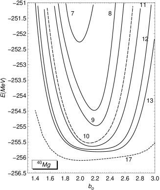
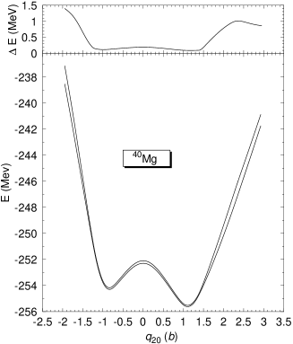
Figure 1: On the left hand side, the ground state HFB energies for $\@@nuc{40}{Mg}$ are plotted as functions of the HO length $b_{o}$ ($b_{\perp}=b_{z}=b_{o}$) for the $N_{Shell}=7,8,9,10,11,12,13$ and 17 bases. The curve corresponding to the basis used in the present work ($N_{Shell}=10$) is plotted as a dashed line. On the right hand side, lower panel, the HFB energies computed with $b_{o}=2.1$ fm and $N_{Shell}=10$ and 11 are plotted as a function of the quadrupole moment. In the upper panel, the energy difference between the $N_{Shell}=10$ and $N_{Shell}=11$ calculations is plotted as a function of the quadrupole moment.

A few words concerning the convergence of our calculations with the size of the HO basis are in order here specially taking into account that we have to deal with the dripline nucleus $\@@nuc{40}{Mg}$. One should note that due to the proximity of the two neutron dripline, the full HFB approximation must be used [83, 9] and absolute convergence for the binding energy can only be found for HO basis with a very large number of shells. At the mean field level such a hard task is still feasible. Even in the case we were interested in a single $q_{20}$ configuration, angular momentum projected calculations with very large $N_{Shell}$ can also be performed. The main reason why we can not consider so large $N_{Shell}$ in the present study is obvious: the enormous amount (typically of the order of one thousand) of angular momentum projected hamiltonian overlaps to be computed in the configuration mixing calculation make the problem intractable. In $\@@nuc{40}{Mg}$ (using the $q_{20}$ range $-2.0b\leq q_{20}\leq 3.0b$, the mesh $\Delta q_{20}=0.1b$ and 16 points in the angular momentum projection) if the basis is increased from $N_{Shell}=10$ to $N_{Shell}=11$ the computational time required to evaluate all the projected kernels increases by a factor of 10 (from 3 days to one month in a typical workstation). Here it is worth to remark that besides the technical difficulties in the configuration mixing calculation, our force is a finite range force and its mathematical structure leads to very complicated matrix elements whose evaluation is very time consuming.

On the other hand, as the absolute value of the binding energy does not affect very much the collective motion (it is only affected by the shape of the energy landscape) we can select a reasonable value of $N_{Shell}$ for which the energy landscape is well converged (i.e. its shape remains almost unchanged in the regions of physical significance when the value of $N_{Shell}$ is increased). As we will see in the next paragraph $N_{Shell}=10$ is more than enough for the present study.

On the left hand side of Fig. 1 we show the ground state HFB energy for $\@@nuc{40}{Mg}$ as a function of the oscillator length $b_{o}$ ($b_{\perp}=b_{z}=b_{o}$) for different values of $N_{Shell}$ (the Coulomb exchange energy is not included). As expected the curves become more and more flat for increasing values of $N_{Shell}$. Already the $N_{Shell}=17$ basis can be considered as a reasonable approximation for an infinite basis in this nucleus as the dependence of the energy on the oscillator length is very weak for a wide range of $b_{o}$ values. For $N_{Shell}=10$ a minimum in the energy curve is obtained for $b_{o}=2.1$. Using the minima of the corresponding energy curves for $N_{Shell}=10$ and $N_{Shell}=17$ we get $E_{N_{Shell}=10}-E_{N_{Shell}=17}=568.37$ keV. In $\@@nuc{38}{Mg}$, the same analysis has been carried out and the overestimation of the energy is 543.29 keV. As a consequence, for the two neutron separation energy $S_{2N}$ it is obtained that $\mid S_{2N,N_{Shell}=10}(^{40}Mg)-S_{2N,N_{Shell}=17}(^{40}Mg)\mid=25.12$ keV. Also a very good agreement is found, in $\@@nuc{40}{Mg}$, between our values for the proton and neutron $\beta_{2}$ deformation parameters $({\beta}_{2}^{Z},{\beta}_{2}^{N})=(0.38,0.31)$ and the ones (0.35, 0.28) of the calculation in coordinate space of Ref. [29]. This can be understood from the fact that our basis roughly corresponds to $R_{box}\approx 9.4fm$ while it was found in Ref. [29] that the deformation parameters remain practically unchanged for $R_{box}\geq 7fm$ in $\@@nuc{40}{Mg}$.

On the right hand side of Fig. 1 we show, in the lower panel, the energy landscapes of $\@@nuc{40}{Mg}$ as a function of the quadrupole moment for the calculations with $N_{Shell}=10$ and $N_{Shell}=11$. In the upper panel we have represented the energy difference between both calculations. From this plots we observe how in the region between -1.5 b and 1.5 b the energy landscape does not change much when the basis is increased. As we will see in another section this range of quadrupole deformation is the one where the collective dynamics is concentrated and therefore it is not expected to find significant differences between the calculations with $N_{Shell}=10$ and $N_{Shell}=11$.

Since the main interest of the present study is focussed on physical quantities like $S_{2N}$ values, rotational energy corrections, excitation energies, etc., and these quantities do not change very much with the number of HO shells, we conclude that our mean field results with $N_{Shell}=10$ can be regarded as a reasonable choice. Even more, the zero point rotational energy correction $E_{ROT}^{I=0}=E_{HFB}-E^{I=0}$ is $\approx$ 3 MeV for the ground state configuration in $\@@nuc{40}{Mg}$, i.e, the zero point rotational energy correction is 5.3 times larger than the relative energy difference $E_{N_{Shell}=10}-E_{N_{Shell}=17}$, and also remains practically unchanged for increasing values of $N_{Shell}$.

Figure 2: Mean field potential energy surfaces for Magnesium isotopes as functions of the axially symmetric quadrupole moment. These curves have been shifted to accommodate them in a single plot. The corresponding energy shifts in panel a) are -85, -65, -50, -35, -25 MeV for $\@@nuc{20-28}{Mg}$, while in panel b) they are -10, -7, -7, -8, -15, -20 MeV for $\@@nuc{30-40}{Mg}$.

In Fig. 2 we show the mean field potential energy surfaces (MFPES) as a function of the axially symmetric quadrupole moment $q_{20}$ for the even-even Magnesium isotopes $\@@nuc{20-40}{Mg}$. The MFPES shown do not include the Coulomb exchange energy and they have been shifted to accommodate them in a single plot (see caption). As one can see, with the exception of $\@@nuc{20}{Mg}$, the MFPES are very flat around the corresponding minima indicating that further correlations could, in some cases, change the conclusions obtained at the mean field level.

The nucleus $\@@nuc{20}{Mg}$ shows a well defined spherical minimum which is a consequence of the N=8 neutron shell closure. On the other hand, both $\@@nuc{22}{Mg}$ and $\@@nuc{24}{Mg}$ are prolate deformed in their ground states. In $\@@nuc{22}{Mg}$ the ground state corresponds to $q_{20}=0.5b({\beta}_{2}=0.40)$ and an oblate local minimum also appears at $q_{20}=-0.2b$ (${\beta}_{2}=-0.17$) with an excitation energy of 1.65 MeV. In the case of $\@@nuc{24}{Mg}$ the ground state corresponds to $q_{20}=0.6b$ (${\beta}_{2}=0.43$) and another local minimum is found at $q_{20}=-0.3b$ (${\beta}_{2}=-0.22$) with an excitation energy of 3.86 MeV. The only oblate isotope in this chain is the nucleus $\@@nuc{26}{Mg}$ whose ground state is located at $q_{20}=-0.4b$ (${\beta}_{2}=-0.26$). A prolate isomeric state is also found at $q_{20}=0.5b$ (${\beta}_{2}=0.32$) with an excitation energy of 707 keV with respect to the oblate ground state. On the other hand, the nuclei $\@@nuc{28}{Mg}$, $\@@nuc{30}{Mg}$ and $\@@nuc{32}{Mg}$ show spherical ground states. The MFPES of both $\@@nuc{28,30}{Mg}$ are particularly flat around their spherical ground states. In the nucleus $\@@nuc{32}{Mg}$ we obtain a prolate shoulder at $q_{20}=0.8b$ (${\beta}_{2}=0.36$) in the MFPES with 1.86 MeV of excitation energy with respect to the spherical ground state.

From $\@@nuc{34}{Mg}$ to the dripline isotope $\@@nuc{40}{Mg}$, prolate deformed ground states are found. The ground state deformations are $q_{20}=0.9b$ $({\beta}_{2}=0.36)$, $q_{20}=0.9b$ $({\beta}_{2}=0.33)$, $q_{20}=1.0b$ $({\beta}_{2}=0.33)$ and $q_{20}=1.1b$ $({\beta}_{2}=0.33)$ in $\@@nuc{34}{Mg}$, $\@@nuc{36}{Mg}$, $\@@nuc{38}{Mg}$ and $\@@nuc{40}{Mg}$, respectively. Besides the fact that prolate configurations become dominant in all these nuclei, one should note that close-lying oblate isomeric states are found in the MFPES of $\@@nuc{36}{Mg}$, $\@@nuc{38}{Mg}$ and $\@@nuc{40}{Mg}$ at $q_{20}=-0.4b$ $({\beta}_{2}=-0.15)$, $q_{20}=-0.6b$ $({\beta}_{2}=-0.20)$ and $q_{20}=-0.8b$ $({\beta}_{2}=-0.25)$ with excitation energies of 2.98 MeV, 2.51 MeV and 1.38 MeV with respect to prolate ground states.

Figure 3: In each panel, proton (thick dashed lines) and neutron (thick full lines) particle-particle correlation energies $-E_{pp}$ are depicted as a function of the quadrupole moment. Also the HFB energy curves are plotted as thin full lines.

In Fig. 3 the proton and neutron particle-particle correlation energies ( defined as $-E_{pp}=\frac{1}{2}Tr\left(\Delta{\kappa}^{*}\right)$) are plotted as a function of the quadrupole deformation for all the isotopes considered. The evolution of the particle-particle correlation energies is well correlated with the structures found in the MFPES. Non-zero proton pairing correlations are found in all the spherical or oblate minima. In addition, sizeable neutron pairing correlations are found in $\@@nuc{22,24}{Mg}$ and in $\@@nuc{36,38,40}{Mg}$ for the spherical and oblate minima. Vanishing proton pairing correlations are found in the prolate side starting at $q_{20}=0.5$b in all the isotopes. The range of quadrupole moments for which the proton pairing correlations vanish increases with the neutron number. An expected result is that neutron pairing correlations vanish in the mean field spherical ground states of both $\@@nuc{20}{Mg}$ and $\@@nuc{32}{Mg}$ as a consequence of the N=8 and N=20 shell closures. However, tangible neutron pairing correlations are found at the spherical configuration of $\@@nuc{40}{Mg}$ pointing to the erosion of the N=28 spherical shell closure already at the mean field level. On the other hand, the lowering of the level density around the ground state of this nucleus ($q_{20}\approx 1b$) leads to vanishing proton and neutron pairing correlations. This agrees with the results of [60, 61, 38] and [59] which suggest that while the N=28 spherical shell closure disappears for some neutron rich nuclei a new deformed shell closure emerges on them.

It should be stressed here that the unphysical collapse of pairing correlations, which is clearly visible from the results of Fig. 3, is one of the main drawbacks of our calculations at the present stage. One should also consider the dynamical pairing correlations in these nuclei and their coupling with the quadrupole degree of freedom in the scope of a theory beyond the mean field in order to treat in an equal footing both short and long range correlations.

Using the absolute minima of the MFPES we have computed the two neutron separation energies $S_{2N}=E_{MF}(Z,N-2)-E_{MF}(Z,N)$ and the results are compared in Fig. 4 with the ones previously obtained in the framework of the mean field approximation with the Skyrme force SIII [29] and SLy4 [30] and with the available experimental values [84]. Our results agree quite well with those of SIII in all the nuclei studied. In the case of SLy4 the agreement is also rather good except for $\@@nuc{22,24}{Mg}$ and $\@@nuc{36}{Mg}$ where the SLy4 results are bigger than ours. The three interactions predict that the nucleus $\@@nuc{40}{Mg}$ is the last bound isotope of the chain. Also the three interactions predict a dip in the $S_{2N}$ of $\@@nuc{34}{Mg}$ and therefore fail to reproduce the peak observed experimentally. The observed peak is usually explained as a consequence of a deformed ground state in $\@@nuc{32}{Mg}$ which has a lower energy than the spherical configuration. As we will see later, the wrong behavior of the $S_{2N}$ of $\@@nuc{34}{Mg}$ at the mean field level is cured when the extra correlation energy (coming from the interplay of the quadrupole fluctuations and the zero point rotational energy corrections) leading to a deformed ground state in $\@@nuc{32}{Mg}$ is considered. Finally, another significant failure of both the Gogny and Skyrme SIII interactions is that of the predicted values of the two neutron separation energies of $\@@nuc{22,24}{Mg}$. As we will see later, considering the zero point rotational energy correction will improve that situation.

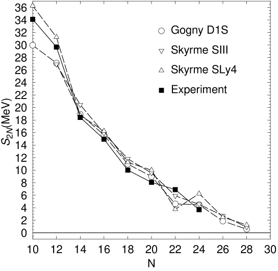
Figure 4: The two neutron separation energies obtained in the present calculations are compared with the experimental data taken from Ref. [84] and with the mean field results obtained with the Skyrme interactions SIII [29] and SLy4 [30].

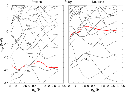
Figure 5: Proton and neutron single particle diagrams as a function of the quadrupole deformation for the nucleus $\@@nuc{32}{Mg}$. Full (dashed) lines correspond to positive (negative) parity levels. The Fermi levels are represented as thick dotted lines.

In Fig. 5 we show the single particle energies for protons and neutrons in $\@@nuc{32}{Mg}$. As in our mean field calculations we solve the full HFB equations, the only quantities that can be properly defined are the quasiparticle energies. However, in order to have the usual Nilsson like diagrams we have chosen to plot the eigenvalues of the mean field Hartree-Fock hamiltonian $h=t+\Gamma$ as a function of the axially symmetric quadrupole deformation. Looking at the neutron single particle energies we observe how at $q_{20}=0.8b$ a couple of $f_{7/2}$ orbitals cross the Fermi surface and become occupied. The occupancy of those orbitals leads to the appearance of the shoulder seen in the MFPES of $\@@nuc{32}{Mg}$. It is also interesting to notice that the almost full occupancy of the $d_{5/2}$ proton orbital favors oblate shapes. In the same way, the full occupancy of the $d_{5/2}$ neutron orbital in $\@@nuc{26}{Mg}$ favors an oblate ground state for this nucleus.

3.2 Correlations beyond the mean field : Angular momentum projection and configuration mixing.

The main outcome of our angular momentum projected calculations is presented in Fig. 6, where the angular momentum projected potential energy surfaces (AMPPES) are shown for the nuclei $\@@nuc{20-40}{Mg}$. The corresponding mean field energy landscapes (dashed curves) are also included for comparison.

The first noticeable fact that one can see is that, with the exception of the $I^{\pi}=0^{+}$ curves, several points around the spherical configuration have been omitted in the AMPPES for the $I\neq 0$ curves. The reason for such omission can be understood by looking at Fig. 7 where the behavior of the projected norm $\mathcal{N}^{I}(q_{20},q_{20})=\langle\phi(q_{20})\mid\hat{P}_{00}^{I}\mid\phi(q_{20})\rangle$ as a function of $q_{20}$ for the nucleus $\@@nuc{32}{Mg}$ is shown. From this figure it becomes clear that the omitted points, in this and the other nuclei, correspond to intrinsic configurations with a very small value of the projected norm $\mathcal{N}^{I}(q_{20},q_{20})$. In those situations the projected energy is the quotient of two very small quantities and therefore its evaluation is affected by numerical inaccuracies that lead to erratic values (deviations from the smooth trend can be as large as a few MeV). Fortunately, due to the smallness of the projected norm, these points can be safely omitted since they do not play any role in the configuration mixing calculations [37, 39, 62, 63, 35, 59] to be discussed later on. We also observe that no energy gain is obtained for the spherical configurations and $I^{\pi}=0^{+}$. From a physical point of view this is the expected behavior since these spherical configurations are already pure $0^{+}$ states as can also be seeing in Fig. 7 where we have $\mathcal{N}^{I=0}(0,0)=1$.

Figure 6: Angular momentum projected potential energy surfaces (full lines) for the nuclei $\@@nuc{20-40}{Mg}$ and for the spin values $I^{\pi}=0^{+},2^{+},4^{+},6^{+}$ as functions of the axially symmetric quadrupole moment $q_{20}$. The mean field potential energy surfaces are also plotted as dashed lines. In the nucleus $\@@nuc{40}{Mg}$ we have also included (dotted lines) the projected results corresponding to the calculation with $N_{shell}=11$.

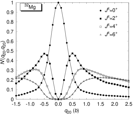
Figure 7: Projected norm $\mathcal{N}^{I}(q_{20},q_{20})$ as a function of $q_{20}$ for the nucleus $\@@nuc{32}{Mg}$. For more details see the main text.

Comparing the MFPES and the $I^{\pi}=0^{+}$ AMPPES of the nuclei $\@@nuc{20}{Mg}$, $\@@nuc{28}{Mg}$, $\@@nuc{30}{Mg}$ and $\@@nuc{32}{Mg}$ one can see that while at the mean field level spherical ground states are obtained, once we carry out angular momentum projection two minima, one prolate and the other oblate, appear. These minima are very close in energy and the difference amounts to around 40, 80, and 49 keV in $\@@nuc{20}{Mg}$, $\@@nuc{28}{Mg}$, $\@@nuc{30}{Mg}$, respectively, and 637 keV in $\@@nuc{32}{Mg}$. These minima are separated by a spherical barrier which is around 1, 3, and 2.6 MeV in $\@@nuc{20}{Mg}$, $\@@nuc{28}{Mg}$, $\@@nuc{30}{Mg}$, respectively, and 1.6 MeV in $\@@nuc{32}{Mg}$.

It is noticeable to observe how the ground state of $\@@nuc{32}{Mg}$ becomes deformed after the inclusion of the rotational energy correction. The intrinsic configuration corresponding to the shoulder seen in the MFPES at $q_{20}=0.8b$ has a big correlation energy coming from the restoration of the angular momentum that is big enough as to overcome the energy difference with the spherical configuration. The deformed intrinsic configuration at $q_{20}=0.8b$ corresponds to (see Fig.5) a configuration in which two neutrons from the $f_{7/2}$ shell have crossed the Fermi surface. In the shell model language this is just a configuration where a pair of neutrons have been promoted from the $sd$ to the $pf$ shell and this is the physical mechanism invoked [41, 43] by the shell model practitioners to explain deformation in this nucleus.

All the other Magnesium isotopes, with the exception made of $\@@nuc{26}{Mg}$ are prolate deformed at $I^{\pi}=0^{+}$. In fact, for increasing spin values the prolate minima become deeper than the oblate ones or the oblate minima are washed out.

The nucleus $\@@nuc{26}{Mg}$, with its oblate intrinsic state at $I^{\pi}=0^{+}$ is the exception in all the Mg isotopes studied. As it was mentioned before, the responsible for such oblate minimum is the full occupancy of the neutron $d_{5/2}$ orbital which favors oblate deformations. The intrinsic state of the lowest lying $I^{\pi}=2^{+}$ state remains oblate deformed but already at $I^{\pi}=4^{+}$ the underlying intrinsic state becomes prolate deformed. The spectroscopic quadrupole moment of the lowest $2^{+}$ state in $\@@nuc{26}{Mg}$ is known experimentally [26] to be -13.5 (20) fm² indicating that this is a prolate deformed state. However, the experimental low excitation energy of the $0^{+}_{2}$ state in this nucleus (3.588 MeV, versus the 6.432 MeV for the same quantity in $\@@nuc{24}{Mg}$) is an indication of a strong shape coexistence between the prolate and oblate solutions.

From the above discussed results we realize that the AMPPES for some nuclei and some spin values show the phenomenon of shape coexistence and therefore, a configuration mixing calculation is needed to disentangle the structure of those states. Even in those situations where the AMPPES show a relatively well pronounced minimum it is always interesting to check its stability in the framework of the configuration mixing calculation. The reason is that not only the AMPPES but also the collective inertia has to be considered in the framework of a dynamical treatment in order to determine the stability of a given solution. With this fact in mind, we have carried out Angular Momentum Projected Generator Coordinate Method (AMPGCM) calculations along the lines described in subsection 2.3 using the intrinsic axial quadrupole moment $q_{20}$ as generating coordinate. These configuration mixing calculations have been performed with a mesh $\Delta q_{20}=10fm^{2}$ which was tested to be accurate enough to describe, at least, the low-lying spectrum we are interested in this study.

Figure 8: Collective wave functions squared for the ground states ($\sigma=1$) and the spin values $I^{\pi}=0^{+},2^{+},4^{+},6^{+}$ of the nuclei $\@@nuc{20,22,24}{Mg}$. The corresponding projected energy curve is also plotted for each spin value. The $y-axis$ scales are in energy units and always span an energy interval of $15$ MeV (minor ticks are $0.5$ MeV apart). The collective wave functions have also been plotted against the energy scale after proper scaling and shifting, that is, the quantity $E^{I,\sigma}+15\times{\mid G^{I,\sigma=1}(q_{20})\mid}^{2}$ is the one actually plotted. With this choice of scales we can read from the figure the energy gain due to the quadrupole fluctuations by considering the position of the wave functions’ tail relative to the projected curve.

Figure 9: The same as Fig. 8 but for the nuclei $\@@nuc{26,28,30}{Mg}$. The y axis scales span in this case an energy interval of$13$ MeV.

Figure 10: The same as Fig. 9 but for the nuclei $\@@nuc{32-40}{Mg}$.

In Figs. 8, 9, and 10 we show the ground state ($\sigma=1$) collective wave functions squared ${\mid G^{I,\sigma=1}(q_{20})\mid}^{2}$ for all the Magnesium isotopes studied in this paper up to $I^{\pi}=6^{+}$. We also plotted in each panel the AMPPES for the corresponding spin value. It is worth pointing out that from the position of the tails of the wave functions relative to the projected energies (see figure caption) we can read the energy gain due to the quadrupole fluctuations. In order to understand in a more quantitative way these collective wave functions it is convenient to analyze [37, 39, 62, 59] the averages

$${\bar{q}_{20}}^{I,\sigma}=\int dq_{20}{\mid G^{I,\sigma}(q_{20})\mid}^{2}q_{20}$$ (41)

that give a measure of the deformation of the underlying intrinsic states.

The $0_{1}^{+}$ wave function for $\@@nuc{20}{Mg}$ shows a great admixture between the prolate and the oblate minima found in the AMPPES. In fact, prolate and oblate configurations have practically the same weight and therefore the ground state of this nucleus is spherical on the average. The energy gain due to quadrupole fluctuations is only 582 keV. As a result, the deformation effects previously found in the AMPPES are not stable once quadrupole fluctuations are taken into account and N=8 remains, on the average, as a spherical magic number. On the other hand for spin values $I^{\pi}\geq 2^{+}$ the ground state collective wave functions are almost inside the prolate wells, with the average deformations $\bar{q}_{20}=0.37b$, $0.53b$ and $0.64b$ for the states $2_{1}^{+}$,$4_{1}^{+}$, and $6_{1}^{+}$ respectively.

For $\@@nuc{22}{Mg}$ and $\@@nuc{24}{Mg}$ the ground state collective wave functions are well inside the prolate wells. This clearly shows on the one hand, the stability of the deformation effects found in the corresponding AMPPES and on the other that both systems are dominated by prolate deformations in the considered spin range. The average deformations are $0.41b$, $0.58b$, $0.62b$ and $0.63b$ for the states $0_{1}^{+}$, $2_{1}^{+}$, $4_{1}^{+}$, and $6_{1}^{+}$ in $\@@nuc{22}{Mg}$, while the corresponding values in $\@@nuc{24}{Mg}$ are $0.59b$, $0.69b$, $0.70b$, and $0.76b$.

In the nucleus $\@@nuc{26}{Mg}$, both the $0_{1}^{+}$ and the $2_{1}^{+}$ states are slightly oblate deformed with ${\bar{q}_{20}}^{I=0,\sigma=1}=-0.17b$ and ${\bar{q}_{20}}^{I=2,\sigma=1}=-0.16b$ while for the state $4_{1}^{+}$ the collective wave function becomes prolate deformed (i.e. a band crossing takes place) with ${\bar{q}_{20}}^{I=4,\sigma=1}=0.39b$ and ${\bar{q}_{20}}^{I=6,\sigma=1}=0.72b$. In both $\@@nuc{28}{Mg}$ and $\@@nuc{30}{Mg}$ the ground state shows considerable mixing between the oblate and prolate configurations. Here for the spin values $I^{\pi}\geq 2^{+}$, the collective wave functions are almost inside the prolate wells. The average deformations are $0.50b$, $0.60b$ and $0.67b$ for $\@@nuc{28}{Mg}$ for the states $2_{1}^{+}$, $4_{1}^{+}$, and $6_{1}^{+}$ while for $\@@nuc{30}{Mg}$ the corresponding deformations for the same spin values are $0.58b$, $0.96b$ and $1.09b$.

The oblate character of the $0^{+}$ and $2^{+}$ states in $\@@nuc{26}{Mg}$ already obtained without configuration mixing is preserved when it is included (although in the latter case almost spherical configurations are obtained), in contradiction with the experimental result (prolate character) extracted from the value of the spectroscopic quadrupole moment of the $2^{+}$ state (-13.5 (20) fm²). However, our results predict a strong shape coexistence for those states in $\@@nuc{26}{Mg}$ as well as for the $0^{+}$ states of $\@@nuc{28-30}{Mg}$. A characteristic fingerprint of shape coexistence comes from the position of the $0^{+}_{2}$ excited state: it is expected to lie at a rather low excitation energy in those situations. Experimentally [25, 26], the excitation energy of the $0^{+}_{2}$ state is known in $\@@nuc{24}{Mg}$ (6.432 MeV), in $\@@nuc{26}{Mg}$ (3.588 MeV) and in $\@@nuc{28}{Mg}$ (3.862 MeV). The sudden drop in the $0^{+}_{2}$ excitation energy in going from $\@@nuc{24}{Mg}$ to $\@@nuc{26}{Mg}$ is a clear indication of shape coexistence in the latter (and also in $\@@nuc{28}{Mg}$) nucleus. In our calculations, apart from the shape of the collective wave functions, we get for those $0^{+}_{2}$ excitation energies the values 5.675, 2.592 and 3.700 MeV for $\@@nuc{24-28}{Mg}$, respectively, that are a clear manifestation of shape coexistence in the last two isotopes. The inclusion of dynamical pairing correlations may improve our description of $\@@nuc{26}{Mg}$. Dynamical pairing correlations for neutrons will not change much the oblate side due to the large single particle gap between the $d_{5/2}$ and the $s_{1/2}$ orbitals (see Fig. 5). However, in the prolate side they can bring into the wave function the $f_{7/2}$ orbital which has a big correlation energy coming from the restoration of the rotational symmetry. As a consequence, the prolate side will gain more energy than the oblate one turning the ground state of $\@@nuc{26}{Mg}$ from slightly oblate to prolate. Although the inclusion of dynamical pairing in the present calculations is rather cumbersome, work along this line is in progress.

Now in $\@@nuc{32}{Mg}$, the $0_{1}^{+}$ collective wave function shows a significant mixing of the oblate and prolate configurations and as a consequence the deformation in the ground state is reduced from the $1.0b$ obtained taking the absolute minimum in the $I^{\pi}=0^{+}$ AMPPES to ${\bar{q}_{20}}^{I=0,\sigma=1}=0.43b$ once quadrupole fluctuations are taken into account via configuration mixing. This shows that the presence of a deformed ground state in this nucleus is the result of a subtle balance between the zero point corrections associated with the restoration of the rotational symmetry and the fluctuations in the collective parameters (in our case the axially symmetric quadrupole moment). On the other hand, the presence of a deformed ground state indicates that for this nucleus N=20 is no longer a magic number. The $2_{1}^{+}$, $4_{1}^{+}$, and $6_{1}^{+}$ wave functions in this nucleus are inside the prolate wells and the average deformations are $0.88b$, $1.01b$ and $1.08b$.

Nucleus	$Q^{spec}(I,\sigma=1)$
	I=2	I=4	I=6
$\@@nuc{20}{Mg}$	-12.59	-23.04	-30.60
$\@@nuc{22}{Mg}$	-17.93	-24.20	-27.41
$\@@nuc{24}{Mg}$	-19.69	-25.14	-28.80
$\@@nuc{26}{Mg}$	2.85 [-11.73]	-15.48	-26.13
$\@@nuc{28}{Mg}$	-15.03 [-15.67]	-21.78	-25.49
$\@@nuc{30}{Mg}$	-13.19 [-12.4]	-27.01	-32.43
$\@@nuc{32}{Mg}$	-19.15 [-18.1]	-26.31	-30.09
$\@@nuc{34}{Mg}$	-20.78 [-22.7]	-27.59	-31.27
$\@@nuc{36}{Mg}$	-19.09 [-19.29]	-24.73	-27.20
$\@@nuc{38}{Mg}$	-18.59 [-19.45]	-24.48	-27.22
$\@@nuc{40}{Mg}$	-20.74 [-21.45]	-26.64	-31.01

Table 1: Ground band spectroscopic quadrupole moments $Q^{spec}(I,\sigma=1)$ in $efm^{2}$ for $I^{\pi}=2^{+},4^{+},6^{+}$ in the nuclei $\@@nuc{20-40}{Mg}$. The Shell Model predictions from [44, 46] are shown in brackets.

From $\@@nuc{34}{Mg}$ to $\@@nuc{40}{Mg}$, the ground state collective wave functions become strongly prolate. The dynamical deformations of the $0_{1}^{+}$ states are $0.79b$, $0.77b$, $0.79b$, and $1.17b$ respectively. In all these nuclei, the $\sigma=1$ collective wave functions are well inside the prolate wells in the whole spin range considered. The dynamical deformation values for the states $2_{1}^{+}$, $4_{1}^{+}$ and $6_{1}^{+}$ are $1.0b$, $1.13b$, $1.19b$ in $\@@nuc{34}{Mg}$, $0.99b$, $1.03b$, $1.05b$ in $\@@nuc{36}{Mg}$, $1.03b$, $1.10b$, $1.14b$ in $\@@nuc{38}{Mg}$ and $1.23b$, $1.25b$, and $1.26b$ in $\@@nuc{40}{Mg}$. The results show the stability of the deformation effects in Magnesium isotopes as we move towards the dripline. Moreover, the presence of a deformed ground state in $\@@nuc{40}{Mg}$ also points towards the erosion of the N=28 shell closure. Contrary to the N=20 case, the erosion of the N=28 shell closure already appears at the mean field level and therefore we can say that it is ”stronger” than for the N=20 case. To summarize, it can be concluded that, while N=8 remains a spherical magic number in the Magnesium isotopic chain, both N=20 and N=28 spherical shell closures do not remain.

Here we will make a few comments on the results obtained in the framework of the configuration mixing approach for the nucleus $\@@nuc{40}{Mg}$ when the basis is increased from $N_{Shell}=10$ to $N_{Shell}=11$. The effect on the projected energy landscapes can be seen in the corresponding panel of Fig. 6 where the $N_{Shell}=11$ curves are plotted as dotted lines. Although there are differences (specially at large absolute values of $q_{20}$ ) between the $N_{Shell}=10$ and $N_{Shell}=11$ curves, these differences are almost independent of the considered spin. Therefore, we do not expect big changes in the excitation energies of the ground state rotational band as is the case: these excitation energies are, for all spin values, around 10 keV higher for $N_{Shell}=11$ than for $N_{Shell}=10$. As a consequence, the transition gamma ray energies remain unaltered by the increase of the basis size. On the other hand, the excitation energies (with respect to the true ground state) of the members of the excited rotational band decrease on the average by 50 keV and therefore, as in the previous case, the intraband gamma ray energies remain the same. From this results we can conclude that our calculations are well converged in terms of the basis size.

The previous results suggest that all the considered nuclei are dominated by prolate deformations. This is clear from the results we have obtained for the average deformation ${\bar{q}_{20}}^{I,\sigma=1}$ and also from the negative values of the ground band spectroscopic quadrupole moments presented in Table 1. With the exception of $\@@nuc{26}{Mg}$, our results for the spectroscopic quadrupole moments show a very good agreement with the Shell Model predictions of Ref.[44, 46] (these predictions are shown in brackets) for the spectroscopic quadrupole moments of the $2_{1}^{+}$ states. Experimentally, the $2^{+}$ spectroscopic quadrupole moment of $\@@nuc{24}{Mg}$ is -16.6 (6) $e^{2}$ fm² [26] and the one of $\@@nuc{26}{Mg}$ is -13.5 (20) $e^{2}$fm² [25]. For $\@@nuc{24}{Mg}$ we obtain a reasonable agreement with experiment (a 15 per cent discrepancy) whereas for $\@@nuc{26}{Mg}$ the disagreement is strong. In the latter case, we have already traced back the disagreement to the strong shape coexistence obtained in our calculations and also to the effect of dynamical pairing correlations (not included in the present work).

The values obtained for the quadrupole moments ${\bar{q}_{20}}^{I,\sigma}$ of the intrinsic states can be used to classify in terms of bands each of the physical states provided by the AMPGCM approach. In Fig. 11 we have plotted the energies of the AMPGCM states $E^{I,\sigma}$ in a diagram of energy versus quadrupole moment. Each energy $E^{I,\sigma}$ is placed at a $q_{20}$ value corresponding to ${\bar{q}_{20}}^{I,\sigma}$. In addition, we have plotted the AMPPES for $I=0$ to guide the eye. Although, in the case of the $\sigma=1$, many of the features observed in this figure have already been discussed, there we also show the results corresponding to the first excited states ($\sigma=2$) provided by the AMPGCM approach. Note that one of the main advantages of such representation is that the band structure of each nucleus can be observed at a glance.

Figure 11: The AMPGCM energies $E^{I,\sigma}$ for $\sigma=1$ and $\sigma=2$ and $I^{\pi}=0^{+},2^{+},4^{+},6^{+}$ are plotted in an energy versus quadrupole moment diagram for the nuclei $\@@nuc{20-40}{Mg}$. The quadrupole moment of each AMPGCM state is given by the average quadrupole moment ${\bar{q}_{20}}^{I,\sigma}$. The AMPPES for $I^{\pi}=0^{+}$ are also plotted to guide the eye.

In Fig. 12 we compare the results for the AMPGCM two neutron separation energies $S_{2N}=E_{0_{1}^{+}}(N-2)-E_{0_{1}^{+}}(N)$ with the corresponding mean field results (see subsection 3.1) and also with the available experimental values [84]. The AMPGCM binding energy is the sum of the mean field binding energy of the intrinsic state plus the energy gain due to the restoration of the rotational symmetry plus the energy gain due to the configuration mixing. Therefore, the differences in the two neutron separation energies obtained in the AMPGCM and the mean field are due to the later two contributions. An analysis of those contributions show that the rotational energy correction is the main responsible for the differences observed in the two neutron separation energies. The AMPGCM $S_{2N}$ energies differ substantially from the mean field ones in the nuclei $\@@nuc{22}{Mg}$ and $\@@nuc{34}{Mg}$ and are much closer to the experiment. On the other hand, it is worth to remark that the nucleus $\@@nuc{40}{Mg}$ remains the last bound isotope in the chain in both theoretical approaches.

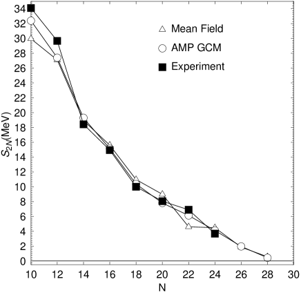
Figure 12: The two neutron separation energies $S_{2N}$ for Magnesium isotopes as obtained in the framework of the AMPGCM are compared with the corresponding mean field values and also with the available experimental values taken from [84]. The AMPGCM $S_{2N}$ are defined as $E_{0_{1}^{+}}(N-2)-E_{0_{1}^{+}}(N)$.

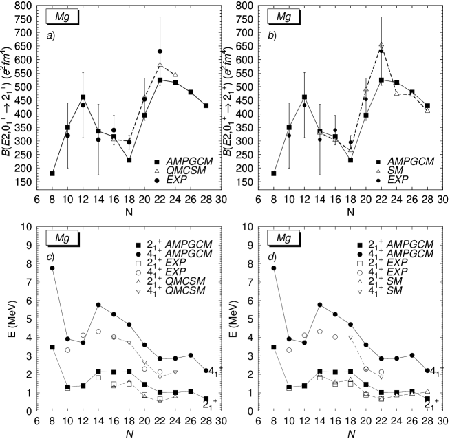
Figure 13: The excitation energies of the states $2_{1}^{+}$ and $4_{1}^{+}$ provided by the AMPGCM and the $B(E2,0^{+}_{1}\rightarrow 2^{+}_{1})$ transition probabilities in $\@@nuc{20-40}{Mg}$ are compared with the available experimental data [25, 15, 16, 22, 19, 20, 23] and with the theoretical predictions of the Quantum Monte Carlo Shell Model [45] and the Shell Model [44, 46].

In Fig. 13 the excitation energies of the $2_{1}^{+}$ and $4_{1}^{+}$ states and the $B(E2,0^{+}_{1}\rightarrow 2^{+}_{1})$ transition probabilities obtained in the framework of the AMPGCM are compared with the available experimental values [25, 15, 16, 22, 19, 20, 23] and also with the predictions of the Quantum Monte Carlo Shell Model [45] and the Shell Model [44, 46]. Concerning the $B(E2)$ transition probabilities we clearly see, from panels a) and b), that the agreement with the available experimental data is rather satisfactory and in most cases (with the exception of $\@@nuc{30}{Mg}$ where our prediction appears a little bit too low) our results stay within the experimental error bars. On the other hand, our results are also consistent with the predictions of the Quantum Monte Carlo Shell Model [45] and the Shell Model [44, 46]. Our results, although not as good as the SM or QMCSM ones, are very satisfactory considering that the parameters of the force have not been fitted to the region and/or the physics of quadrupole collectivity and also that no effective charges have been used in our calculations of the transition probabilities.

The calculated excitation energies for the $2_{1}^{+}$ and $4_{1}^{+}$ states are plotted in panels c) and d). They reproduce quite well the experimental isotopic trend and are again consistent with the theoretical trends predicted by both the Shell Model [44, 46] and the Quantum Monte Carlo Shell Model [45]. In most cases, however, our values come too high as compared with the experiment. In our previous works [37, 59] we also noticed the same behavior in some N $\approx$ 20 and N $\approx$ 28 nuclei (our predictions were too high as compared with the experiment). Probably a proper treatment of some missing correlations will give the quenching factors we need for a much better agreement with the experiment. Although it is very difficult to assert before hand what are the missing correlations, the mixing of different $K$ values with a full triaxial angular momentum projection and a beyond mean field treatment of the dynamical pairing fluctuations can be important ingredients for a more realistic description of the nuclei studied in this paper. Another source of discrepancy could be related to the fact that ours is a calculation of the Projection After Variation (PAV) type instead of the more complete Projection Before the Variation (PBV). Having all this in mind and the free parameter character of our calculation we conclude that our results for the excitation energies of the $2_{1}^{+}$ and $4_{1}^{+}$ states show a rather satisfactory agreement with the available experimental and are consistent with other theoretical predictions.

4 Conclusions.

With the aim to describe the phenomenology of quadrupole deformation in light nuclei we have performed calculations with the Gogny force and in the framework of beyond mean field theories for the nuclei $\@@nuc{20-40}{Mg}$. First of all, the results show the fundamental role played by the angular momentum projection for a proper description of the physics under study. The effect of projection in all the physical observables is so big that it can not be overlooked as it has been common practice in many previous calculations. In addition, we also find that the effect of configuration mixing is in most cases rather relevant. From our results we conclude that for the Magnesium isotopes the N=8 shell closure is preserved whereas for N=20 and N=28 deformed ground states appear in the calculations. The three isotopes from $\@@nuc{36Mg}{t}$o the drip line nucleus $\@@nuc{40}{Mg}$ are predicted to be prolate deformed in their ground states. Concerning the excitation energies and $B(E2)$ transition probabilities of the low-lying excited states we obtain a reasonable agreement with experiment. The agreement is not as good as the one obtained with other approaches like the Shell Model or the Quantum Monte Carlo Shell model. The reason for that probably lies in the fact that our treatment of the problem, although it contains the most important ingredients, is not as refined and complete as the one of the SM and/or the QMCSM. In addition, the interaction used has not been fitted to this specific region of the periodic table. The later could be consider as a drawback of our calculations but we think it is the other way around and in fact is a manifestation of the strong predicting power of the Gogny interaction. It is rather satisfactory to obtain the results presented in this paper with an interaction that is also able to reproduce, for instance, the fission barrier heights of $\@@nuc{240}{Pu}$.

Finally, the consistency of the prescription used for the density dependent term of the interaction in the present calculations beyond mean field has been discussed in great detail.

5 Appendix A: Calculation of transition probabilities.

In this appendix we present the basic formulas for the computation of angular momentum projected transition probabilities in the framework of the AMPGCM. The starting point is the transformation property of the multipole operators $\hat{Q}_{\lambda\mu}$ under rotations

$$\hat{R}(\Omega)\hat{Q}_{\lambda\mu}\hat{R}^{\dagger}(\Omega)=\sum_{{\mu}^{{}^{\prime}}}\mathcal{D}_{{\mu}^{{}^{\prime}}\mu}^{\lambda}(\Omega)\hat{Q}_{\lambda{\mu}^{{}^{\prime}}}$$ (42)

Using the well known result for the product of two Wigner functions [74] as well as the definition of Eq. (2) for the angular momentum projection operator and the property

$$\hat{P}_{MK^{{}^{\prime}}}^{I}\hat{P}_{K{{}^{\prime}}M{{}^{\prime}}}^{I^{\prime}}={\delta}_{II{{}^{\prime}}}{\delta}_{KK{{}^{\prime}}}\hat{P}_{MM{{}^{\prime}}}^{I}$$ (43)

we obtain after some algebra the result

$$\hat{P}_{K_{f}M_{f}}^{I_{f}}\hat{Q}_{\lambda\mu}\hat{P}_{M_{i}K_{i}}^{I_{i}} = \langle I_{i}M_{i}\lambda{\mu}\mid I_{f}M_{f}\rangle$$ (44)

$$\times {\sum}_{\nu{\mu}^{{}^{\prime}}}(-)^{{\mu}^{{}^{\prime}}-\mu}\langle I_{i}\nu\lambda{\mu}^{{}^{\prime}}\mid I_{f}K_{f}\rangle\hat{Q}_{\lambda{\mu}^{{}^{\prime}}}\hat{P}_{\nu K_{i}}^{I_{i}}.$$

With the definition of the projected wave functions of Eq. (1) and the previous result we obtain

$$\langle\Psi_{I_{f}M_{f}}(\vec{q}_{f})\mid\hat{Q}_{\lambda\mu}\mid\Psi_{I_{i}M_{i}}(\vec{q}_{i})\rangle=\frac{\langle I_{i}M_{i}\lambda{\mu}\mid I_{f}M_{f}\rangle}{\sqrt{2I_{f}+1}}\langle I_{f}\vec{q}_{f}\mid\mid\hat{Q}_{\lambda}\mid\mid I_{i}\vec{q}_{i}\rangle$$ (45)

with

$$\langle I_{f}\vec{q}_{f}\mid\mid \hat{Q}_{\lambda}\mid\mid I_{i}\vec{q}_{i}\rangle=\frac{(2I_{i}+1)(2I_{f}+1)}{8{\pi}^{2}}(-)^{I_{i}-\lambda}\sum_{K_{i}K_{f}\nu{\mu}^{{}^{\prime}}}(-)^{K_{f}}g_{K_{f}}^{I_{f}*}(\vec{q}_{f})g_{K_{i}}^{I_{i}}(\vec{q}_{i})$$ (48)

$$\times \left(\begin{array}[]{ccc}I_{i}&\lambda&I_{f}\\ \nu&{\mu}^{{}^{\prime}}&-K_{f}\end{array}\right)\int d\Omega\mathcal{D}_{\nu K_{i}}^{I_{i}*}(\Omega)\langle\varphi(\vec{q}_{f})\mid\hat{Q}_{\lambda{\mu}^{{}^{\prime}}}\hat{R}(\Omega)\mid\varphi(\vec{q}_{i})\rangle$$

Using now the expression (28) we get

$$\langle\Phi_{I_{f}M_{f}}({\sigma}_{f})\mid\hat{Q}_{\lambda\mu}\mid\Phi_{I_{i}M_{i}}({\sigma}_{i})\rangle=\frac{\langle I_{i}M_{i}\lambda{\mu}\mid I_{f}M_{f}\rangle}{\sqrt{2I_{f}+1}}$$

$$\times\int d\vec{q}_{i}d\vec{q}_{f}f^{I_{f},{\sigma}_{f}*}(\vec{q}_{f})\langle I_{f}\vec{q}_{f}\mid\mid\hat{Q}_{\lambda}\mid\mid I_{i}\vec{q}_{i}\rangle f^{I_{i},{\sigma}_{i}}(\vec{q}_{i}).$$ (49)

Finally, the expression for the $B(E\lambda,{I_{i}}{{\sigma}_{i}}\rightarrow{I_{f}}{{\sigma}_{f}})$ transition probability is written as

$$B(E\lambda ,{I_{i}}{{\sigma}_{i}}\rightarrow{I_{f}}{{\sigma}_{f}})=\frac{e^{2}}{2I_{i}+1}\sum_{M_{i}M_{f}\mu}\left|\langle\Phi(I_{f},M_{f},{\sigma}_{f})\mid\hat{Q}_{\lambda\mu}\mid\Phi(I_{i},M_{i},{\sigma}_{i})\rangle\right|^{2}$$ (50)

$$= \frac{e^{2}}{2I_{i}+1}\left|\int d\vec{q}_{i}d\vec{q}_{f}f^{I_{f},{\sigma}_{f}*}(\vec{q}_{f})\langle I_{f}\vec{q}_{f}\mid\mid\hat{Q}_{\lambda}\mid\mid I_{i}\vec{q}_{i}\rangle f^{I_{i},{\sigma}_{i}}(\vec{q}_{i})\right|^{2}$$

In the present work we are interested in the calculation of transition probabilities for axially symmetric HFB states labelled by the quadrupole deformation $q_{20}$. Taking advantage of the axial symmetry of the intrinsic wave function as well as the selfconsistent symmetry $e^{-i\pi\hat{J}_{y}}$ we can simplify the above expressions as follows. First we have

$$\langle\varphi(q_{20,f})\mid\hat{Q}_{\lambda{\mu}^{{}^{\prime}}}\hat{R}(\Omega)\mid\varphi(q_{20,i})\rangle=e^{i\alpha{\mu}^{{}^{\prime}}}\langle\varphi(q_{20,f})\mid\hat{Q}_{\lambda{\mu}^{{}^{\prime}}}e^{-i\beta\hat{J}_{y}}\mid\varphi(q_{20,i})\rangle$$ (51)

that leads to

$$\int d\Omega\mathcal{D}_{QK_{i}}^{I_{i}*}(\Omega)\langle\varphi(q_{20,f})\mid\hat{Q}_{\lambda{\mu}^{{}^{\prime}}}\hat{R}(\Omega)\mid\varphi(q_{20,i})\rangle=4{\pi}^{2}{\delta}_{Q-{\mu}^{{}^{\prime}}}{\delta}_{K_{i}0}$$ (52)

$$\int_{0}^{\pi}d\beta\sin(\beta)d_{-{\mu}^{{}^{\prime}}0}^{I_{i}*}(\beta)\langle\varphi(q_{20,f})\mid\hat{Q}_{\lambda{\mu}^{{}^{\prime}}}e^{-i\beta\hat{J}_{y}}\mid\varphi(q_{20,i})\rangle$$

Applying this result to the expression of Eq. (48) we obtain

$$\langle I_{f}q_{20,f}\mid\mid\hat{Q}_{\lambda}\mid\mid I_{i}q_{20,i}\rangle=\frac{(2I_{i}+1)(2I_{f}+1)}{2}(-)^{I_{i}-\lambda}\sum_{{\mu}^{{}^{\prime}}}\left(\begin{array}[]{ccc}I_{i}&\lambda&I_{f}\\ -{\mu}^{{}^{\prime}}&{\mu}^{{}^{\prime}}&0\end{array}\right)$$

$$\times \int_{0}^{\pi}d\beta\sin(\beta)d_{-{\mu}^{{}^{\prime}}0}^{I_{i}*}(\beta)\langle\varphi(q_{20,f})\mid\hat{Q}_{\lambda{\mu}^{{}^{\prime}}}e^{-i\beta\hat{J}_{y}}\mid\varphi(q_{20,i})\rangle$$

$$= (2I_{i}+1)(2I_{f}+1)(-)^{I_{i}-\lambda}\frac{1+(-)^{I_{i}}}{2}\sum_{{\mu}^{{}^{\prime}}}\left(\begin{array}[]{ccc}I_{i}&\lambda&I_{f}\\ -{\mu}^{{}^{\prime}}&{\mu}^{{}^{\prime}}&0\end{array}\right)$$ (58)

$$\times \int_{0}^{\frac{\pi}{2}}d\beta\sin(\beta)d_{-{\mu}^{{}^{\prime}}0}^{I_{i}*}(\beta)\langle\varphi(q_{20,f})\mid\hat{Q}_{\lambda{\mu}^{{}^{\prime}}}e^{-i\beta\hat{J}_{y}}\mid\varphi(q_{20,i})\rangle$$ (59)

where we have, in the last line, reduced the integration interval to half the original one.

Finally, from the previous expressions for the axially symmetric case, the $B(E2,{I_{i}}{{\sigma}_{i}}\rightarrow{I_{f}}{{\sigma}_{f}})$ in the framework of the AMPGCM can be written as

$$B(E2 {I_{i}}{{\sigma}_{i}}\rightarrow{I_{f}}{{\sigma}_{f}})=\frac{e^{2}}{2I_{i}+1}$$ , (60)

$$\times \left|\int dq_{20,i}dq_{20,f}f^{I_{f},{\sigma}_{f}*}(q_{20,f})\langle I_{f}q_{20,f}\mid\mid\hat{Q}_{2}\mid\mid I_{i}q_{20,i}\rangle f^{I_{i},{\sigma}_{i}}(q_{20,i})\right|^{2}$$

with

$$\langle I_{f}q_{20,f} \mid\mid\hat{Q}_{2}\mid\mid I_{i}q_{20,i}\rangle=(2I_{i}+1)(2I_{f}+1)\sum_{{\mu}^{{}^{\prime}}}\left(\begin{array}[]{ccc}I_{i}&2&I_{f}\\ -{\mu}^{{}^{\prime}}&{\mu}^{{}^{\prime}}&0\end{array}\right)$$ (63)

$$\times \int_{0}^{\frac{\pi}{2}}d\beta\sin(\beta)d_{-{\mu}^{{}^{\prime}}0}^{I_{i}*}(\beta)\langle\varphi(q_{20,f})\mid\hat{Q}_{2{\mu}^{{}^{\prime}}}e^{-i\beta\hat{J}_{y}}\mid\varphi(q_{20,i})\rangle$$ (64)

References

- [1] W.Nazarewicz, B. Sherril, I.Tanihata, and P. Van Duppen, Nuclear Physics News 6 (1996) 17.
- [2] J. Dobaczewski and W. Nazarewicz, Phil. Trans. R. Soc. Lond. A356 (1998) 2007.
- [3] I. Tanihata, Nucl. Phys. A654 (1999) 235c.
- [4] T. Uchiyama and H. Morinaga, Z. Phys. A320 (1985) 273.
- [5] I. Tanihata, Journ. of Phys. G22 (1996) 157.
- [6] M. Yokoyama, T. Otsuka, and N. Fukunishi, Phys. Rev. C 52 (1995) 1122.
- [7] A. Mueller and B. Sherril, Ann. Rev. Nucl. Part. Sci. 43 (1993) 529.
- [8] W. Nazarewicz, T. R. Werner, and J. Dobaczewski, Phys. Rev. C 50 (1994) 2860.
- [9] J. Dobaczewski, W. Nazarewicz, T.R. Werner, J.F. Berger, C.R. Chinn, and J.Dechargé, Phys. Rev. C 53 (1996) 2809.
- [10] S. Mizutori, J. Dobaczewski, G. A. Lalazissis, W. Nazarewicz, and P.-G.Reinhard, Phys. Rev. C 61 (2000) 044326.
- [11] C.Thibault, R. Klapisch, C. Rigaud, A. M. Poskanzer, R. Prieels, L. Lessard, and W. Reisdorf, Phys. Rev. C12 (1975) 644.
- [12] X. Campi, H. Flocard, A. K. Kerman, and S. Koonin, Nucl. Phys. A251 (1975) 193.
- [13] F. Touchard , J. M. Serre, S. Büttgenbach, P. Guimbal, R. Klapisch, M. de Saint Simon, C. Thibault, H. T. Duong, P. Juncar, S. Liberman, J. Pinard, and J. L. Vialle, Phys. Rev. C 25 (1982) 2756.
- [14] T.Motobayashi, Y.Ikeda, Y.Ando, K.Ieki, M.Inoue, N.Iwasa, T.Kikuchi, M.Kurokawa, S.Moriya, S.Ogawa, H.Murakami, S.Shimoura, Y.Yanagisawa, T.Nakamura, Y.Watanabe, M.Ishihara, T.Teranishi, H.Okuno, and R.F.Casten, Phys. Lett. B346 (1995) 9.
- [15] C. Détraz, D. Guillemaud, G. Huber, R. Klapisch, M. Langevin, F. Naulin, C. Thibault, L. C. Carraz, and F. Touchard, Phys. Rev. C 19 (1979) 164.
- [16] D. Guillemaud-Mueller, C. Détraz, M. Langevin, F. Naulin, M. De Saint-Simon, C. Thibault, F. Touchard, and M. Epherre, Nucl. Phys. A426 (1984) 37.
- [17] B. V. Pritychenko, T. Glasmacher, B. A. Brown, P. D. Cottle, R. W. Ibbotson, K. W. Kemper, L. A. Riley, and H. Scheit, Phys. Rev. C 63 (2000) 011305(R).
- [18] H. Iwasaki, T. Motobayashi, H. Sakurai, K. Yoneda, T. Gomi, N. Aoi, N. Fukuda, Zs. Fülöp, U. Futakami, Z. Gacsi, Y. Higurashi, N. Imai, N. Iwasa, T. Kubo, M. Kunibu, M. Kurokawa, Z. Liu, T. Minemura, A. Saito, M. Serata, S. Shimoura, S. Takeuchi, Y. X. Watanabe, K. Yamada, Y. Yanagisawa, K. Yogo, and M. Ishihara, Phys. Lett. B522 (2001) 227.
- [19] F. Azaiez et al., Proceedings of the International Conference Nuclear Structure 98, edited by C. Baktash, AIP Conf. Proc. Vol. 481 (AIP, New York, 1999) p. 243.
- [20] K. Yoneda, H. Sakurai, T. Gomi, T. Motobayashi, N. Aoi, N. Fukuda, U. Futakami, Z. Gacsi, Y. Higurashi, N. Imai, N. Iwasa, H. Iwasaki, T. Kubo, M. Kunibu, M. Kurokawa, Z. Liu, T. Minemura, A. Saito, M. Serata, S. Shimoura, S. Takeuchi, Y. X. Watanabe, K. Yamada, Y. Yanagisawa, K. Yogo, A. Yoshida, and M. Ishihara, Phys. Lett. B499 (2001) 233.
- [21] D. Habs, O. Kester, G. Bollen, L. Liljeby, K. G. Rensfelt, D. Schwalm, R. von Hahn, G. Walter, and P. Van Duppen, Nucl. Phys. A616 (1997) 29c.
- [22] B. V. Pritychenko, T. Glasmacher, P.D. Cottle, M. Fauerbach, R.W. Ibbotson, K.W. Kemper, V. Maddalena, A. Navin, R. Ronningen, A. Sakharuk, H. Scheit, and V.G. Zelevinsky, Phys. Lett. B461 (1999) 322.
- [23] S. Raman et al., At. Data Nucl. Data Tables 42 (1991) 1.
- [24] R. W. Ibbotson, T. Glasmacher, B. A. Brown, L. Chen, M. J. Chromik, P. D. Cottle, M. Fauerbach, K. W. Kemper, D. J. Morrissey, H. Scheit, and M. Thoennessen, Phys. Rev. Lett. 80 (1998) 2081.
- [25] P. M. Endt, Nucl. Phys. A521 (1990) 1.
- [26] P. M. Endt, J. Blachot, R. B. Firestone, and J. Zipkin, Nucl. Phys. A633 (1998), 1.
- [27] Z. Ren, Z. Y. Zhu, Y. H. Cai, and G. Xu, Phys. Lett. B380 (1996) 241.
- [28] G. A. Lalazissis, A. R. Farhan, and M. M. Sharma, Nucl. Phys. A628 (1998) 221.
- [29] J. Terasaki, H. Flocard, P. -H. Heenen, and P. Bonche, Nucl. Phys. A621 (1997) 706.
- [30] M. V. Stoitsov, J. Dobaczewski, P. Ring, and S. Pittel, Phys. Rev. C 61 (2000) 034311.
- [31] M. Barranco and R. J. Lombard, Phys. Lett. B78 (1978) 542.
- [32] R. Bengtsson, P. Moller, J. R. Nix, and J. Zhang, Phys. Scr. 29 (1984) 402.
- [33] J. F. Berger, J. P. Delaroche, M. Girod, S. Péru, J. Libert, and I. Deloncle, Inst. Phys. Conf. Ser. 132 (1993) 487.
- [34] P. -G. Reinhard, D. J. Dean, W. Nazarewicz, J. Dobaczewski, J. A. Maruhn, and M. R. Strayer, Phys. Rev. C 60 (1999) 014316.
- [35] P.-H. Heenen, P. Bonche, S. Cwiok, W. Nazarewicz, and A. Valor, Riken Review 26 (2000) 31.
- [36] R. Rodríguez Guzmán, J. L. Egido, and L. M. Robledo, Phys. Lett. B474 (2000) 15.
- [37] R. Rodríguez Guzmán, J. L. Egido, and L. M. Robledo, Phys. Rev. C 62 (2000) 054319.
- [38] S. Péru, M. Girod, and J. F. Berger, Eur. Phys. J. A9 (2000) 35.
- [39] R. Rodríguez Guzmán, J. L. Egido, and L. M. Robledo, Acta Phys. Pol. B 32 (2001) 2385.
- [40] E. K. Warburton, J. A. Becker, and B. A. Brown, Phys. Rev. C 41 (1990) 1147.
- [41] A. Poves and J. Retamosa, Phys. Lett. B184 (1987) 311.
- [42] N. Fukunishi, T. Otsuka, and T. Sebe, Phys. Lett. B296 (1992) 279.
- [43] A. Poves and J. Retamosa, Nucl. Phys. A571 (1994) 221.
- [44] E. Caurier, F. Nowacki, A. Poves, and J. Retamosa, Phys. Rev. C 58 (1998) 2033.
- [45] Y. Utsuno, T. Otsuka, T. Mizusaki, and M. Honma, Phys. Rev. C 60 (1999) 054315.
- [46] E. Caurier, F. Nowacki and A. Poves, Nucl. Phys. A693 (2001) 374.
- [47] M. Lewitowicz, Yu. E. Penionzhkevich, A. G. Artukh, A. M. Kalinin, V. V. Kamanin, S. M. Lukyanov, Nguyen Hoai Chau, A. C. Mueller, D. Guillemaud-Mueller, R. Anne, D. Bazin, C. Détraz, D. Guerreau, M. G. Saint-Laurent, V. Borrel, J. C. Jacmart, F. Pougheon, A. Richard, and W. D. Schmidt-Ott, Nucl. Phys. A496 (1989) 477.
- [48] O. Sorlin , D. Guillemaud-Mueller, A. C. Mueller, V. Borrel, S. Dogny, F. Pougheon, K.-L. Kratz, H. Gabelmann, B. Pfeiffer, A. Wöhr, W. Ziegert, Yu. E. Penionzhkevich, S. M. Lukyanov, V. S. Salamatin, R. Anne, C. Borcea, L. K. Fifield, M. Lewitowicz, M. G. Saint-Laurent, D. Bazin, C. Détraz, F.-K. Thielemann, and W. Hillebrandt, Phys. Rev. C 47 (1993) 2941.
- [49] H. Scheit, T. Glasmacher, B. A. Brown, J. A. Brown, P. D. Cottle, P. G. Hansen, R. Harkewicz, M. Hellström, R. W. Ibbotson, J. K. Jewell, K. W. Kemper, D. J. Morrissey, M. Steiner, P. Thirolf, and M. Thoennessen, Phys. Rev. Lett. 77 (1996) 3967.
- [50] T. Glasmacher et al., Phys. Lett. B395 (1997) 163.
- [51] T. Glasmacher, Nucl. Phys. A630 (1998) 278c.
- [52] R. W. Ibbotson, T. Glasmacher, P. F. Mantica, and H. Scheit, Phys. Rev. C 59 (1999) 642.
- [53] F. Sarazin, H. Savajols, W. Mittig, F. Nowacki, N. A. Orr, Z. Ren, P. Roussel-Chomaz, G. Auger, D. Baiborodin, A. V. Belozyorov, C. Borcea, E. Caurier, Z. Dlouhý, A. Gillibert, A. S. Lalleman, M. Lewitowicz, S. M. Lukyanov, F. de Oliveira, Y. E. Penionzhkevich, D. Ridikas, H. Sakuraï, O. Tarasov, and A. de Vismes, Phys. Rev. Lett. 84 (2000) 5062.
- [54] T. R. Werner, J. A. Sheikh, W. Nazarewicz, M.R. Strayer, A. S. Umar, and M. Misu, Phys. Lett. B335 (1994) 259.
- [55] T. R. Werner, J.A. Sheikh, M. Misu, W. Nazarewicz, J. Rikovska, K. Heeger, A.S. Umar, and M.R. Strayer, Nucl. Phys. A597 (1996) 327.
- [56] D. Hirata, K. Sumiyoshi, B.V. Carlson, H. Toki and I. Tanihata, Nucl. Phys. A609 (1996) 131.
- [57] G. A. Lalazissis, D. Vretenar, P. Ring, M. Stoitsov, and L. M. Robledo, Phys. Rev. C 60 (1999) 014310.
- [58] B. V. Carlson and D. Hirata, Phys. Rev. C62 (2000) 054310.
- [59] R. Rodríguez Guzmán, J. L. Egido, and L. M. Robledo, Phys. Rev. C 65 (2002) 024304.
- [60] P. D. Cottle and K. W. Kemper, Phys. Rev. C 58 (1998) 3761.
- [61] J. Retamosa, E. Caurier, F. Nowacki, and A. Poves, Phys. Rev. C 55 (1997) 1266.
- [62] R. Rodríguez Guzmán, J. L. Egido and L. M. Robledo, Phys. Rev. C 62 (2000) 054308.
- [63] A. Valor, P.-H. Heenen, and P. Bonche, Nucl. Phys. A671 (2000) 145.
- [64] J. Dechargé and D. Gogny, Phys. Rev. C 21 (1980) 1568.
- [65] J. F. Berger, M. Girod and D. Gogny, Nucl. Phys. A428 (1984) 23c.
- [66] P. Ring and P. Schuck, The nuclear many body problem (Springer, Berlin, 1980).
- [67] K. W. Schmid, F. Grümmer, and A. Faessler, Phys. Rev. C 29 (1984) 291.
- [68] K. W. Schmid, F. Grümmer, and A. Faessler, Phys. Rev. C 29 (1984) 308.
- [69] K. Hara, A. Hayashi, and P. Ring, Nucl. Phys. A385 (1982) 14.
- [70] K. Hara and Y. Sun, Int. J. Mod. Phys. E 4 (1995) 637.
- [71] K. Enami, K. Tanabe and N. Yoshinaga, Phys. Rev. C 59 (1999) 135.
- [72] P. Bonche, J. Dobaczewski, H. Flocard, P.-H. Heenen, and J. Meyer, Nucl. Phys. A510 (1990) 466.
- [73] R. E. Peierls and I. Yoccoz, Proc. Phys. Soc. London A70 (1957) 381.
- [74] D. A. Varshalovich, A. N. Moskalev and V. K Khersonskii, Quantum Theory of Angular Momentum (World Scientific, Singapore, 1988).
- [75] A. Valor, J. L. Egido and L. M. Robledo, Phys. Rev. C53 (1996) 172.
- [76] A. Valor, J. L. Egido and L. M. Robledo, Phys. Lett. B392 (1997) 249.
- [77] D. L. Hill and J. A. Wheeler, Phys. Rev. 89 (1953) 1102.
- [78] L. M. Robledo, Phys. Rev. C 50 (1994) 2874.
- [79] J. L. Egido, L. M. Robledo and Y. Sun, Nucl. Phys. A560 (1993) 253.
- [80] R. G. Nazmitdinov, L. M. Robledo, P. Ring and J. L. Egido, Nucl. Phys. A596 (1996) 53.
- [81] R. Balian and E. Brezin, Nuovo Cimento B64 (1969) 37.
- [82] K. Neeargard and E. Wüst, Nucl. Phys. A402 (1983) 311.
- [83] J. Dobaczewski, H. Flocard, and J. Treiner, Nucl. Phys. A422 (1984) 103.
- [84] G. Audi and A. H. Wapstra, Nucl. Phys. A595 (1995) 409.