Perturbative Effective Theory in an Oscillator Basis?

Abstract

The effective interaction/operator problem in nuclear physics is believed to be highly nonperturbative, requiring extended high-momentum spaces for accurate solution. We trace this to difficulties that arise at both short and long distances when the included space is defined in terms of a basis of harmonic oscillator Slater determinants. We show, in the simplest case of the deuteron, that both difficulties can be circumvented, yielding highly perturbative results in the potential even for modest ($\sim$ 6$\hbar\omega$) included spaces.

There is an extensive literature on attempts to relate the effective interaction, needed in any description of nuclei based on a finite set of low-momentum basis states, to the underlying, more singular $NN$ interaction. As Barrett [1] has summarized, one hope of investigators in the 1970s was that $H^{eff}$ might be expanded perturbatively in either the bare potential $V$ or in the $G$ matrix, the sum of all two-nucleon ladder diagrams for scattering in the excluded, high-momentum space. While some phenomenological success was achieved by selecting certain diagrams [2], more systematic treatments provided little indication of convergence. For example, the third-order calculations of Barrett and Kirson [3] yielded a correction of the same size but opposite in sign to the second-order result. At about the same time Shucan and Weidenmuller [4] demonstrated in a toy model that strongly coupled “intruder” states – states low in energy having little overlap with the model space – generically lead to poorly convergent expansions. These disappointing results led many practioners to turn to phenomenological $H^{eff}$s – an approach that is also lacking because it fails to provide a basis for generating effective operators consistent with $H^{eff}$.

The lack of a first-principles technique for effective interactions had a discouraging effect on the field for a number of years. However several recent developments – including the rapid growth of computing power and interest in effective field theory [5] – have encouraged new attempts to calculate $H^{eff}$ in a systematic, controlled way.

One step in this direction was reported recently [6]: for an included space consisting of a complete set of harmonic oscillator (HO) Slater determinants of energy $\leq\Lambda_{SM}\hbar\omega$, the deuteron and ³He were treated as exact effective theories (ET). The point was to illustrate crucial aspects of ETs that are generally absent in models like the shell model (SM), including nontrivial wave function normalizations, the many-body nature of effective interactions, the rapid evolution of $H^{eff}$ matrix elements with changes in the model space, and the crucial role of consistent effective operators.

The starting point for the calculation of Ref. [6] is the Bloch-Horowitz equation [7]. For a low-momentum “included space” defined by $\Lambda_{SM}$ and a HO size parameter $b$, $H^{eff}$ will be translationally invariant. (Note $\hbar\omega=\hbar^{2}/Mb^{2}$, with $M$ the nucleon mass.) Defining the projection operator onto the high-momentum Slater determinants by $Q(\Lambda_{SM},b)$, one finds

$$H^{eff} = H+H{1\over E-QH}QH$$ (1)

$$H^{eff}|\psi_{SM}\rangle = E|\psi_{SM}\rangle~{}~{}~{}~{}|\psi_{SM}\rangle=(1-Q)|\psi\rangle$$ (2)

where $|\psi\rangle$ is the exact wave function, $H|\psi\rangle=E|\psi\rangle$, and $H=T+V$ is the sum of relative kinetic energy and potential terms. This equation has to be solved self-consistently for each desired but unknown eigenvalue $E$. The method introduced in [6] provided an efficient solution to the self-consistency problem, constructing the needed Green’s function as a function of $E$ by a method based on the Lanczos algorithm: with this technique one iteratively extracts the high-momentum spectral information most relevant to the construction of the Green’s function.

This approach, in principle, can be extended to heavier systems. In practice, however, the integration over high-momentum states becomes more challenging with increasing $A$: in [6], where the Argonne $v18$ potential [8] was employed, high-momentum integrations up to $\Lambda_{\infty}\sim 140$ ($\sim$ 60) were necessary to achieve 1 keV (25 keV) accuracy. In this letter we argue that this integration can be performed in a much simpler way.

We begin by investigating why the high momentum integration is nonperturbative. One can envision moving the SM scale $\Lambda_{SM}$ very close to the necessary $\Lambda_{\infty}$, which clearly makes the excluded-space contribution to the BH equation a small correction. As the energy denominator in Eq. (1) is then very large, one might assume that the high-momentum problem is now perturbative.

To test this conclusion we expand the excluded-space contribution to Eq. (1)

$$H{1\over E-QH}QH=H\left[{1\over E-QT}+{1\over E-QT}QV{1\over E-QT}+...\right]QH$$ (3)

The order-by-order results ( dashed lines in Fig. 1a) are quite curious. The total excluded-space contribution, given the very high value of $\Lambda_{SM}$ = 70 chosen, accounts for only 20 keV of binding energy; 85% of this is generated by the first term in Eq. (2). However subsequent order-by-order corrections appear to converge to a value a few keV above the true binding energy. Only after $\sim$ 1000 orders of perturbation theory is the correct binding energy slowly achieved. (Very similar results are obtained if one uses the HO Hamiltonian $T+V_{0}$, instead of $T$, as the unperturbed Hamiltonian.)

In Figs. 1b and 1c this behavior is explored for two matrix elements of $H^{eff}$. Most matrix elements converge rapidly, like the $1s-1s$ example of Fig. 1b. The exceptions are those where the bra or ket lies in the last included shell, i.e., $\Lambda_{\alpha}=\Lambda_{SM}$, such as the $n=36$ $s$-state case of Fig 1c). This associates the poor convergence with $T$ which, because of the raising/lowering properties of the gradient operator in a HO basis, connects only such states to the excluded space.

It is helpful to note that a HO-basis ET differs from effective field theories in that the expansion is around an intermediate momentum $q_{0}\sim 1/b$, rather than $q_{0}\sim 0$. Fig. 1 shows that this expansion then induces a familiar long-distance problem: because HO wave functions fall off too sharply, the correct asymptotic wave function can only be achieved by scattering through a very large number of high-momentum oscillator states. Consequently a poorly convergent “tail” exists regardless of how high $\Lambda_{SM}$ is chosen: a larger $\Lambda_{SM}$ restricts the unresolved tail to larger $r$ and thus limits its numerical significance, but does not in principle make the problem perturbative.

The solution to this problem is not entirely trivial. The HO basis is essential because of the center-of-mass separability it provides. Because the relevant operator is the relative kinetic energy

$$T={1\over 2}\sum_{i\neq j=1}^{A}T_{ij}$$ (4)

where $T_{ij}=(\vec{p}_{i}-\vec{p}_{j})^{2}/2AM$, the missing long-distance correlations are two-body. As the problem is associated with $T$ hopping from the included space at large $r$ with a large amplitude, we rearrange the BH equation so that the Green’s function is sandwiched between $V$s, thereby cutting off large-$r$ propagation [9]

$$\langle\alpha|H^{eff}|\beta\rangle=\langle\alpha|T|\tilde{\beta}\rangle+\langle\tilde{\alpha}|V+V{1\over E-QH}QV|\tilde{\beta}\rangle$$ (5)

where

$$|\tilde{\alpha}\rangle={E\over E-QT}|\alpha\rangle$$ (6)

with $|\alpha\rangle$ a HO Slater determinant. Thus $|\alpha\rangle=|\tilde{\alpha}\rangle$ for Slater determinants for which $\Lambda_{\alpha}\neq\Lambda_{SM}$. Otherwise, apart from the overall normalization, $|\tilde{\alpha}\rangle$ differs significantly from $|\alpha\rangle$ only in its large-$r$ behavior (Fig. 2). We stress that Eq. (4) is equivalent to Eq. (1). Finally we insert the bracketed Green’s function expansion of Eq. (2) into Eq. (4). Thus $QV$ always appears between insertions of $QT$, summed to all orders.

The results are given by the solid lines in Figs. 1a and 1c. The $\langle 36s|H^{eff}|36s\rangle$ matrix element and total binding energy now converge rapidly. In fact $\Lambda_{SM}$ can be lowered to $\sim 40$ while keeping high momentum contributions perturbative: in third order 1 keV accuracy is maintained.

However, with further lowering of the SM scale, the convergence again exhibits hints of deterioration – with new symptoms. For $\Lambda_{SM}=30$, the third-order calculation reduces $\sim$ 10% errors in the bare value of $\langle 1s|H^{eff}|1s\rangle$ to $\sim 0.2$%. But an error in excess of 0.1% – corresponding to 50 keV – persists after 10 additional orders of perturbation. Unlike the case discussed above, all matrix elements are affected, though the nonperturbative corrections to $s-s$ transitions are larger than those for $s-d$ and much larger than those for $d-d$ matrix elements. This is a signature of scattering at small $r$ through the hard core. Numerically one can verify that the nonperturbative tail disappears if the hard core in $V$ is removed.

An exact ET must yield the same result regardless of the choice of excluded space parameters $b$ and $\Lambda_{SM}$. However it is possible that a judicious choice of these parameters might simplify the numerical difficulty of the ET. While $\Lambda_{SM}$ generally is limited by the size of one’s computer, $b$ can be varied freely. A natural choice for $b$ is the value that minimizes the 0th order energy (obtained by ignoring entirely the last term in Eq. (1) or Eq. (4)). This corresponds to minimizing the bare Hamiltonian $\langle T+V\rangle_{SM}$ as a function of $b$ in Eq. (1). The closer the binding energy to the correct value, of course, the smaller the contribution of the high-momentum corrections due to scattering in the excluded space.

The dashed lines in Fig. 3 are the 0th-order energies for Eq. (1) as a function of $b$ for $\Lambda_{SM}$ = 6, 8, and 10. As $\langle T+V\rangle_{SM}$ is a variational estimate of the energy, the contour minima are upper bounds to the exact result. The 0th-order results fail to bind the deuteron; the minima are achieved for $b\sim$ 0.79-0.83$f$. (Note that $b_{eff}=\sqrt{2}b$ is the size scale in the relative coordinate, $\vec{r_{1}}-\vec{r_{2}}$.) This $b_{eff}$ is considerably smaller than the nuclear size: the SM is doing its best to find a compromise between two needs, resolving the hard core (a problem that becomes easier for small $b$) and reproducing the correct long-distance behavior (a problem that becomes easier for large $b$ - a doubling of $b$ roughly halves the number of high-momentum states that must be included to calculate $T^{eff}$ to an equivalent accuracy). The resulting compromise $b$ addresses neither need well.

The solid lines in Fig. 3 are the corresponding results for the 0th-order approximation to Eq. (4). The minima shift to $b\sim$ 0.4-0.5$f$, and the unperturbed results are very accurate, with errors of 21, 36, and 52 keV for 10, 8, and 6 $\hbar\omega$ spaces – an improvement of about a factor of 100 in binding-energy accuracy over the corresponding dashed-line results. This has been achieved without taking into account any effects of $QV$. The interpretation is clear: once one has solved the long-distance problem through the resummation of Eq. (4), the nonperturbative effects (as we shall see below) of the hard core can be absorbed almost entirely into the included space, given an appropriate HO size scale $b\sim r_{c}$, where $r_{c}$ is the hard-core radius. This scale arises naturally out of the minimization, because the short-range repulsion is such a dominant feature of the potential.

The $4\hbar\omega$ 0th-order energy minimum is not quite so impressive: the included space is sufficiently restrictive that a nonnegligible contribution from $QV$ remains even if $b$ is optimized. Conversely, the minimum at 10$\hbar\omega$ is very flat, which means that there is a range of $b$ – a set of included spaces – in which the effects of $QV$ remain very small.

Fig. 4 gives our most important results. Fig. 4a illustrates the problem noted in the introduction, a perturbative expansion of Eq. (1) converges very poorly. Only at 10 $\hbar\omega$ (not shown) do the fluctuations begin to damp out, though they remain at the $\sim$ 100 keV level even at high orders. In contrast, the expansion based on Eq. (4) (Fig. 4b) is highly perturbative. The 1st-order correction $V(E-QT)^{-1}QV$ for the 6,8, and 10 $\hbar\omega$ calculations yields binding energies accurate to $\mathrel{\hbox to0.0pt{\lower 4.0pt\hbox{\hskip 1.0pt$\sim$}\hss}\raise 1.0pt\hbox{$<$}}$3 keV. We see that the 10 and 8 $\hbar\omega$ calculations are effectively identical at and beyond 2nd order; the 10, 8, and 6 $\hbar\omega$ results merge at 4th order. Even the $4\hbar\omega$ 0th-order result is quickly corrected to an accuracy of 1.2 keV at 3rd order.

The accuracy of the unperturbed $10\hbar\omega$ result of Eq. (4) is comparable to that achieved in [6] by direct summation of the high-momentum contribution to Eq. (1) to $\Lambda_{\infty}\sim 70$. Perhaps more important, however, is the promising result that the remaining corrections associated with $QV$ are perturbative. This has important implications for the complexity of $H^{eff}$ in heavier nuclei, suggesting that the number of nucleons in the excluded space that must be linked by $QV$ can be limited. For example, $V(E-QT)^{-1}QV$ links only three nucleons. Rapid convergence in the perturbation expansion translates into a hierarchy of three-body, four-body, etc, contributions to $V^{eff}$ of rapidly diminishing importance.

So far the discussion has emphasized results and their interpretation rather than technical aspects. However, the technical aspects deserve discussion because many HO properties can be usefully exploited:

1) The operator $T$ is diagonal in a plane wave basis. The transformation into that basis is particularly simple for the HO, as the Fourier transform of a HO is a HO.

2) The operator appearing in the Green’s function, however, is $QT$, which is more difficult to treat. One can relate this Green’s function to the free Green’s function $G_{0}={1\over E-T}$, at the cost of a matrix inversion in the included space. Using the included-space projector $P=1-Q$ we define operators acting within the included space

$$\Gamma_{0}=PG_{0}P,~{}~{}\Gamma_{1}=PG_{0}VG_{0}P,~{}~{}\Gamma_{2}=PG_{0}VG_{0}VG_{0}P~{}~{}...$$ (7)

One can then write the perturbative expansion of $H^{eff}$ as

$$H^{eff} = (E-\Gamma_{0}^{-1})+\Gamma_{0}^{-1}\Gamma_{1}\Gamma_{0}^{-1}+\Gamma_{0}^{-1}(\Gamma_{2}-\Gamma_{1}\Gamma_{0}^{-1}\Gamma_{1})\Gamma_{0}^{-1}$$ (8)

$$+ \Gamma_{0}^{-1}(\Gamma_{3}-\Gamma_{1}\Gamma_{0}^{-1}\Gamma_{2}-\Gamma_{2}\Gamma_{0}^{-1}\Gamma_{1}+\Gamma_{1}\Gamma_{0}^{-1}\Gamma_{1}\Gamma_{0}^{-1}\Gamma_{1})\Gamma_{0}^{-1}+...$$ (9)

where the terms correspond to the contributions from $T$, $V$, $(QV)^{2}$, $(QV)^{3}$, …, respectively. Note that the matrix $\Gamma_{0}^{-1}$ differs from the matrix $P(E-T)P$ only in the entries where the bra and ket belong to the last included “shell”.

3) As $T$ is a sum over all relative momenta, an evaluation of $G_{0}$ in an independent-particle basis will generate a product of two-particle correlations (with a dependence on each relative partial wave). In contrast, with Jacobi coordinates $G_{0}$ is diagonal in momentum space

$$G_{0}={1\over E-{1\over 2M}(\dot{k}_{1}^{2}+...+\dot{k}_{A-1}^{2})}$$ (10)

where $\dot{k}_{i}$ is the momentum associated with the $i$th Jacobi coordinate. Clearly the Jacobi basis is the simpler choice. As noted before, if we work to some order in perturbation theory, then the number of nucleons interacting at one time in the excluded space will be limited. Thus, in general, there will be “spectator” nucleons, and the matrix element will have a spectator dependence corresponding to the overlap integral weighted by $\Gamma_{0}$. The importance of such spectator dependence in a HO-based ET was noted in [10]. The integrals over spectator nucleons can be handled analytically and are reducible to finite sums over gamma and incomplete gamma functions.

These properties allow one to evaluate the HO matrix elements of the operators of Eq. (7), and thus the binding energy term by term in perturbation theory. In the present case of the deuteron the relative-coordinate matrix element is transformed into momentum space

$$\langle n_{f}(\ell_{f}s)jmtm_{t}|\Gamma_{\alpha}(E)|n_{i}(\ell_{i}s)jmtm_{t}\rangle={(-1)^{n_{f}+n_{i}+\alpha+1}\over\hbar\omega_{eff}}\left[{4(n_{f}-1)!(n_{i}-1)!\over\Gamma(n_{f}+\ell_{f}+1/2)\Gamma(n_{i}+\ell_{i}+1/2)}\right]^{1/2}$$ (11)

$$\times\int_{0}^{\infty}d\rho_{f}{\rho_{f}^{\ell_{f}+2}e^{\rho_{f}^{2}/2}\over\rho_{f}^{2}+E_{0}}L_{n_{f}-1}^{\ell_{f}+1/2}(\rho_{f}^{2})\int_{0}^{\infty}d\rho_{i}{\rho_{i}^{\ell_{i}+2}e^{\rho_{i}^{2}/2}\over\rho_{i}^{2}+E_{0}}L_{n_{i}-1}^{\ell_{i}+1/2}(\rho_{i}^{2})\langle\rho_{f}(\ell_{f}s)jmtm_{t}|V_{\alpha}|\rho_{i}(\ell_{i}s)jmtm_{t}\rangle$$ (12)

where $\omega_{eff}=\omega/2$, $L$ is a Laguerre polynomial, and $E_{0}$ is the dimensionless binding energy $|E|/\hbar\omega_{eff}$. The momentum-space matrix element of the iterated potential is given by a simple recursion relation

$$\langle\rho_{f}(\ell_{f}s)jmtm_{t}|V_{\alpha}|\rho_{i}(\ell_{i}s)jmtm_{t}\rangle = \sum_{\tilde{\ell}}\int_{0}^{\infty}d\tilde{\rho}{\tilde{\rho}^{2}\over\tilde{\rho}^{2}+E_{0}}\langle\rho_{f}(\ell_{f}s)jmtm_{t}|V_{1}|\tilde{\rho}(\tilde{\ell}s)jmtm_{t}\rangle$$ (13)

$$\times \langle\tilde{\rho}(\tilde{\ell}s)jmtm_{t}|V_{\alpha-1}|\rho_{i}(\ell_{i}s)jmtm_{t}\rangle$$ (14)

where $\langle\rho_{f}(\ell_{f}s)jmtm_{t}|V_{1}|\tilde{\rho}(\tilde{\ell}s)jmtm_{t}\rangle$ is given by

$${1\over\hbar\omega_{eff}}\int_{0}^{\infty}drr^{2}\sqrt{{2\over\pi}}j_{\ell_{f}}(\rho_{f}r)\langle(\ell_{f}s)jmtm_{t}|V(rb_{eff})|(\tilde{\ell}s)jmtm_{t}\rangle\sqrt{{2\over\pi}}j_{\tilde{\ell}}(\tilde{\rho}r)$$ (15)

Note that all integration variables are dimensionless.

In summary we have shown that conventional HO-basis effective interactions calculations involve both long- and short-distance nonperturbative scattering. The effects of such scattering can be absorbed into the included space by an appropriate summation of the relative kinetic energy to all orders, followed by a tuning of the HO included space to absorb most of the hard-core scattering. This tuning results from minimizing the 0th-order energy as a function of $b$. In the test case of the deuteron, we find very accurate 0th order results and very rapid convergence in further orders of perturbation. Existing Jacobi coordinate SM codes can treat light $1p$-shell nuclei and three-body interactions [11], which should allow similar calculations to be done through 1st-order in the two-body potential (0th order in the weaker three-body potential) in these cases.

We thank Bob Wiringa for providing the $v18$ potential codes, and Silas Beane and Martin Savage for helpful discussions. This work was supported in part by US Department of Energy grants DE-FG03-00ER41132 and DE-FC02-01ER41187.

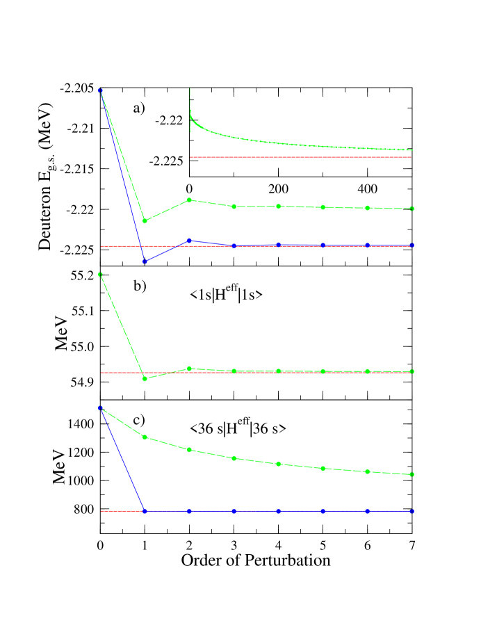
FIG. 1.: The dash lines were obtained by inserting the Green’s function expansion of Eq. (2) into Eq. (1). Very slow convergence is found for the binding energy (a) and for the effective matrix elements that involve included states in the last “shell.” Other matrix elements (b) converge quickly. The corresponding results for Eq. (4) (solid lines) all converge rapidly. The horizontal lines are the exact results.

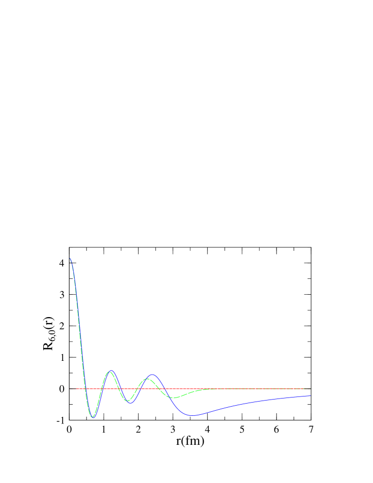
FIG. 2.: For $\Lambda_{SM}=10$ the last included s-state has $n=6$. The state $E/(E-QT)|n=6\ell=0\rangle$ (solid line) is compared to its HO counterpart, $|n=6\ell=0\rangle$ (dashed line), showing that the former is modified at large distances. The modified wave function was multiplied by 1.934 to match the HO at $r=0$.

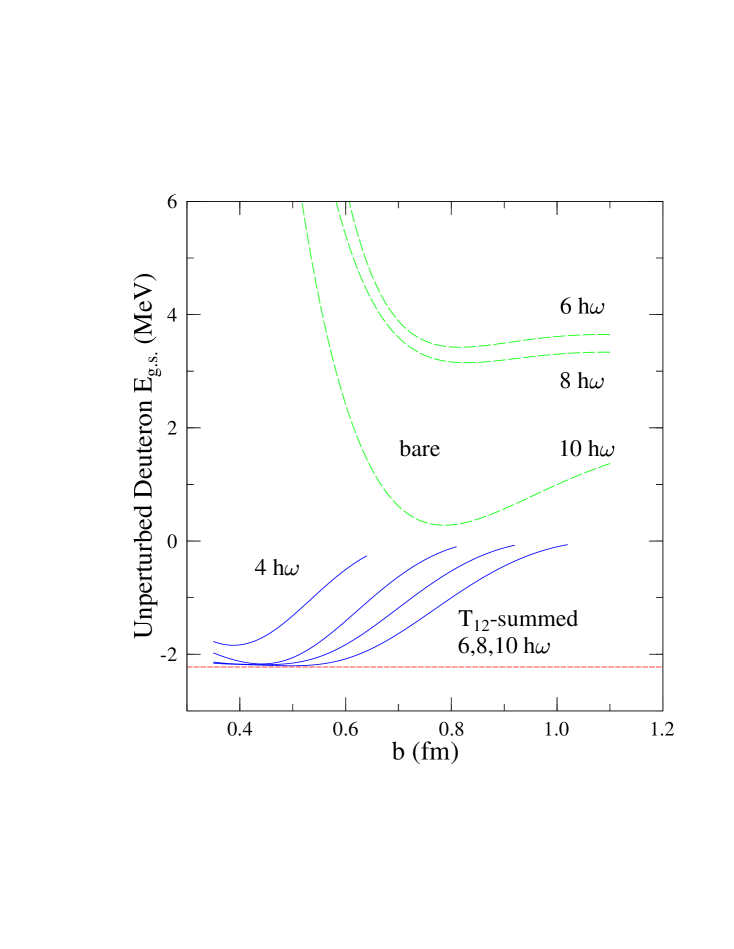
FIG. 3.: The 0th order approximations to Eq. (1) (dashed lines) and Eq. (4) (solid lines) as a function of $b$, showing the shifts in the minima and improved binding energies associated with the latter.

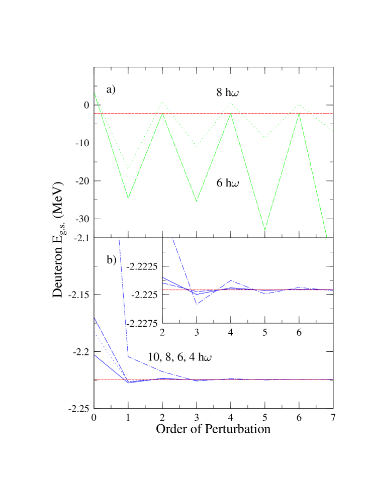
FIG. 4.: Binding energies obtained by treating the excluded-space contributions to Eq. (1) (a) and Eq. (4) (b) perturbatively, via the Green’s function expansion of Eq. (2). The solid, dotted, dashed, and dot-dashed lines correspond to 10, 8, 6, and 4 $\hbar\omega$ included spaces, respectively.

REFERENCES

- [1] B. R. Barrett, Czech. J. Phys. 49, 1 (1999).
- [2] T. T. S. Kuo and G. E. Brown, Nucl. Phys. 85, 40 (1966); T. T. S. Kuo, Nucl. Phys. A103, 1 (1967).
- [3] B. R. Barrett and M. W. Kirson, Nucl. Phys. A148, 145 (1970).
- [4] T. H. Shucan and H. A. Weidenmuller, Ann. Phys. (N.Y.) 73, 108 (1972) and 76, 483 (1973).
- [5] S. R. Beane et al., in the Boris Ioffe Festschrift, ed. M. Shifman (World Scientific, Singapore, 2001), vol. 1, pp. 133-269.
- [6] W. C. Haxton and C.-L. Song, Phys. Rev. Lett. 84, 5484 (2000).
- [7] C. Bloch and J. Horowitz, Nucl. Phys. 8, 91 (1958).
- [8] R. B. Wiringa, V. G. J. Stoks, and R. Schiavilla, Phys. Rev. C51, 38 (1995).
- [9] This equation is also the appropriate form into which phenomenological contact interactions can be inserted, representing the missing short-range physics. See W. C. Haxton and T. Luu, Nucl. Phys. A690, 15 (2001).
- [10] D. C. Zheng et al., Phys. Rev. C52, 2488 (1995); N. Barnea, W. Leidemann, and G. Orlandini, Phys. Rev. C61, 054001 (2000).
- [11] P. Navratil et al., Phys. Rev. C61, 044001 (2000); T. Luu, P. Navratil, and W. C. Haxton, in preparation.