An Algebraic Pairing Model with $Sp(4)$ Symmetry and its Deformation

Abstract

A fermion realization of the compact symplectic $sp(4)$ algebra provides a natural framework for studying isovector pairing correlations in nuclei. While these correlations manifest themselves most clearly in the binding energies of $0^{+}$ ground states, they also have a large effect on the energies of excited states, including especially excited $0^{+}$ states. In this article we consider non-deformed as well as deformed algebraic descriptions of pairing through the reductions of $sp_{(q)}(4)$ to different realizations of $u_{(q)}$(2) for single-$j$ and multi-$j$ orbitals. The model yields a classification scheme for completely paired $0^{+}$ states of even-even and odd-odd nuclei in the $1d_{3/2}$, $1f_{7/2}$, and $1f_{5/2}2p_{1/2}2p_{3/2}1g_{9/2}$ shells. Phenomenological non-deformed and deformed isospin-breaking Hamiltonians are expressed in terms of the generators of the dynamical symmetry groups $Sp(4)$ and $Sp_{q}(4)$. These Hamiltonians are related to the most general microscopic pairing problem, including isovector pairing and isoscalar proton-neutron interaction along with non-linear interaction in the deformed extension. In both the non-deformed and deformed cases the eigenvalues of the Hamiltonian are fit to the relevant Coulomb corrected experimental $0^{+}$ energies and this, in turn, allows us to estimate the interaction strength parameters, to investigate isovector-pairing properties and symmetries breaking, and to predict the corresponding energies. While the non-deformed theory yields results that are comparable to other theories for light nuclei, the deformed extension, which takes into account higher-order interactions between the particles, gives a better fit to the data. The multi-shell applications of the model provide for reasonable predictions of energies of exotic nuclei.

1 Introduction

The pairing problem, which was introduced first in atomic physics [1], was later applied to nuclear physics [2, 3] in an attempt to describe binding energies of nuclei and their low-lying vibrational spectra [4, 5]. Recently, there has been renewed interest in this problem because of new experimental studies of exotic nuclei with relatively large proton excess or with $N\approx Z$. This revival of interest in pairing follows from the recent development of radioactive beam facilities and attempts to bridge from nuclear structure considerations to astrophysical phenomena [6, 7].

Along with approximate mean field solutions (for a review see [8]), the pairing problem can be solved exactly by means of various group theoretical methods, which allow one to explore the underlying symmetries. The $SU(2)$ seniority model [9, 10, 11] provides for a good description of nuclei with large proton or neutron excess, where the like-particle pairing plays a dominant role. The simple “quasi-spin” ($SU(2)\sim Sp(2)$) approach [12] not only offers an elegant way to understand the results from the conventional seniority scheme [1, 2, 13], based on $U(2j+1)\supset Sp(2j+1)\supset SO(3)$, but allows for a straightforward expansion to $SO(5)\sim Sp(4)$ to include protons and neutrons, which otherwise has proven to be too complicated. The generalization to the $SO(5)$ model [14, 15, 16, 17] introduces a relation between identical-particle and proton-neutron ($pn$) isovector (isospin $\tau=1$) pairing modes. The addition of an isoscalar ($\tau=0$) $pn$ pairing channel is described within the framework of the $SO(8)$ model [18, 19, 20] and the Interacting Boson Model ($IBM$) [21].

In the limit of dominant isovector $pn$ pairing correlations, a simple $SO(5)$ seniority model [22, 23] is suitable. Our goal is to investigate properties of the isovector pairing interaction within the context of a fermion realization of the symplectic $sp(4)$ algebra [which is isomorphic to $so(5)$]. The model space consists of $J^{\pi}=0^{+}$ states with pairs coupled to isospin $\tau=1$; mixing with $\tau=0$ $pn$ pairs is not included. The importance of the isovector pairing for binding energies is suggested by experimental data, namely a $\tau=1$ ground state for most $N=Z$ odd-odd nuclei with mass number $A>40$ [24, 25, 26], and by the results of various theoretical studies [27, 28, 29, 30, 31, 32, 33, 34].

While coupling to the isoscalar $pn$ pairing mode may be important in some cases [35, 36], we exclude – to the best of our ability – the ground states of nuclei that show fingerprints of isoscalar pairing correlations. In short, the $Sp(4)$ model is applied to $0^{+}$ ground states of even-$A$ nuclei and to the higher-lying $0^{+}$ isobaric analog states in most of odd-odd nuclei. We refer to these states as isovector-paired states. In this regard, it is important to note that the two-body interaction includes an isoscalar term in addition to the dominant isovector pairing interaction. The isoscalar $pn$ force is related to the symmetry energy and is diagonal in the isovector-paired basis states with good isospin [37]. Diagonal high-$J$ components of the nuclear interaction are also present in the model. The shell structure and its dimension play an important role in the construction of the fermion pairs and their interaction in accordance with the Pauli principle. The isovector pairing term is assumed to be particle-hole symmetric, which enters naturally in points to a decrease in energy with respect to the mean-field solution of a no-pair theory [38].

Limiting cases of $sp(4)$ correspond to different reductions of $sp(4)$ to $u(2)$ and show distinct properties of different coupling modes of the isovector pairing interaction; specifically, proton-neutron ($pn$) and like-particle ($pp$ and $nn$) pairing phenomena. The theory provides for a classification of nuclear states with respect to the number valence protons and neutrons occupying a major shell. The notion of a dynamical symmetry extends this picture to include an isospin-breaking phenomenological interaction which is related to a general microscopic Hamiltonian for the pairing problem. The final result can be written in terms of the second order invariants of the subalgebras of $sp(4)$ which then reduces the problem to an exactly solvable theory.

A $q$-deformation of the classical algebraic structure is introduced. A quantum extension of the dynamical symmetry approach is realized leading also to an exact $q$-deformed solution of the problem and its limiting cases. The motivation behind the $q$-deformed generalization is that, as a novel and richer model, it allows us to include non-linear features of the interaction and to investigate the respective changes this may require in the strength parameters and in the pairing gaps. Existing applications of the $q$-deformed algebraic structures to the pairing problem [39] are restricted mainly to the $SU_{q}(2)$ limit [40, 41] of the dynamical symmetry approach presented here for $Sp_{q}(4)$.

Fully-paired even-even and odd-odd nuclei, $32\leq A\leq 100$, in $1d_{3/2}$, $1f_{7/2}$ and $1f_{5/2}2p_{1/2}2p_{3/2}1g_{9/2}$ orbitals are considered in details in this investigation. An analysis of the results, obtained by fitting model parameters to experimental data both in the deformed and non-deformed cases, provides for a reasonable prediction of the relevant $0^{+}$ state energies of nuclei classified as belonging to a major shell and gives insight into their pair structure and isospin mixing. It also estimates the broad limits of applicability of such a simple algebraic model and its deformed non-linear extension– which is in agreement with the results of other theoretical approaches for describing pairing phenomena in nuclear systems [13, 22, 37, 42, 43, 44].

The paper is organized as follows. In the next section, the algebraic structure of the fermion realization of $sp(4)$ and its deformation $sp_{q}(4)$ is introduced with emphasis on the physical interpretation of the generators. In Section 3 the application of the algebraic constructions is realized through the introduction of a model Hamiltonian in both the deformed and non-deformed cases. In Section 4, the parameters of the Hamiltonians are presented as output of a fitting procedure to the respective experimental energies and the results are analyzed. A summary of our findings and the main conclusions as well as possible further developments of the approach are discussed in the final section.

2 Algebraic structure of non-deformed and q-deformed $sp(4)$

To introduce notation, we start with a brief review of the algebraic structures that enter into the discussion [45]. The $sp(4)$ algebra is realized in terms of the creation (annihilation) fermion operator $c_{m,\sigma}^{\dagger}$ ($c_{m,\sigma}$) $\sigma=\pm 1,$ where these operators create (annihilate) a particle of type $\sigma$ in a state of total angular momentum $j=\frac{1}{2},\frac{3}{2},\frac{5}{2},...,$ with projection $m$ along the $z$ axis ($-j\leq m\leq j$). They satisfy Fermi anticommutation relations

$$\begin{array}[]{ll}\{c_{m^{\prime},\sigma^{\prime}},c_{m,\sigma}^{\dagger}\}=\delta_{m^{\prime},m}\delta_{\sigma^{\prime},\sigma}&\{c_{m^{\prime},\sigma^{\prime}}^{\dagger},c_{m,\sigma}^{\dagger}\}=\{c_{m^{\prime},\sigma^{\prime}},c_{m,\sigma}\}=0\end{array}$$ (1)

and Hermitian conjugation is given by $(c_{m,\sigma}^{\dagger})^{*}=c_{m,\sigma}.$ For a given $\sigma,$ the dimension of the fermion space is $2\Omega_{j}=2j+1.$

The deformation of the $sp_{q}(4)$ algebra is introduced in terms of $q$-deformed creation and annihilation operators $\alpha_{m,\sigma}^{\dagger}$ and $\alpha_{m,\sigma},$ $(\alpha_{m,\sigma}^{\dagger})^{*}=\alpha_{m,\sigma}$, where $\alpha_{m,\sigma}^{(\dagger)}\rightarrow c_{m,\sigma}^{(\dagger)}$ in the limit $q\rightarrow 1.$ The deformed single-particle operators are defined through their anticommutation relation for every $\sigma$ and $m$ [45]:

$$\begin{array}[]{ll}\{\alpha_{m,\sigma},\alpha_{m^{\prime},\sigma}^{\dagger}\}_{q^{\pm 1}}=q^{\pm\frac{N_{\sigma}}{2\Omega_{j}}}\delta_{m,m^{\prime}}&\{\alpha_{m,\sigma},\alpha_{m^{\prime},\sigma^{\prime}}^{\dagger}\}=0,~{}\sigma\neq\sigma^{\prime}\\ \{\alpha_{m,\sigma}^{\dagger},\alpha_{m^{\prime},\sigma^{\prime}}^{\dagger}\}=0&\{\alpha_{m,\sigma},\alpha_{m^{\prime},\sigma^{\prime}}\}=0,\end{array}$$ (2)

where by definition the $q$-anticommutator is given as $\left\{A,B\right\}_{q^{k}}=AB+q^{k}BA.$ A property with physics impact is the dependence of the deformed anticommutation relations on the shell dimension and the operators that count the number of particles, $N_{\pm 1}=\sum_{m=-j}^{j}c{{{{}_{m,\pm 1}^{\dagger}}}}c{{}_{m,\pm 1}}.$

Generators of the symplectic group – The generators of $Sp(4)$ and $Sp_{q}(4)$ are expressed in terms of non-deformed [14, 46] and deformed single-particle operators [45], respectively,

$$\left.\begin{array}[]{l}A_{\frac{\sigma+\sigma^{\prime}}{2}}=\frac{1}{\sqrt{2\Omega_{j}(1+\delta_{\sigma,\sigma^{\prime}})}}\sum_{m=-j}^{j}{{(-1)}^{j-m}}c_{m,\sigma}^{\dagger}c_{-m,\sigma^{\prime}}^{\dagger}\\ B_{\frac{\sigma+\sigma^{\prime}}{2}}=\frac{1}{\sqrt{2\Omega_{j}(1+\delta_{\sigma,\sigma^{\prime}})}}\sum_{m=-j}^{j}{{(-1)}^{j-m}}c{{}_{-m,\sigma}}c{{}_{m,\sigma^{\prime}}}\end{array}\right\}\begin{array}[]{c}non-\\ deformed\end{array}$$ (3)

$$\left.\begin{array}[]{l}F_{\frac{\sigma+\sigma^{\prime}}{2}}=\frac{1}{\sqrt{2\Omega_{j}(1+\delta_{\sigma,\sigma^{\prime}})}}\sum_{m=-j}^{j}{{(-1)}^{j-m}}\alpha_{m,\sigma}^{\dagger}\alpha_{-m,\sigma^{\prime}}^{\dagger}\\ G_{\frac{\sigma+\sigma^{\prime}}{2}}=\frac{1}{\sqrt{2\Omega_{j}(1+\delta_{\sigma,\sigma^{\prime}})}}\sum_{m=-j}^{j}{{(-1)}^{j-m}}\alpha{{}_{-m,\sigma}}\alpha{{}_{m,\sigma^{\prime}}}\end{array}\right\}\begin{array}[]{c}deformed\end{array}$$ (4)

where $\sigma,\ \sigma^{\prime}=\pm 1$ and $A_{0,\pm 1}=(B_{0,\pm 1})^{\dagger},\ F_{0,\pm 1}=(G_{0,\pm 1})^{\dagger}$. These operators create (annihilate) a pair of fermions coupled to total angular momentum and parity $J^{\pi}=0^{+}$ [14, 2] and thus constitute boson-like objects. The rest of the generators of $Sp(4)$ are $D_{\sigma,\sigma^{\prime}}=\frac{1}{\sqrt{2\Omega_{j}}}\sum_{m=-j}^{j}c{{{{}_{m,\sigma}^{\dagger}}}}c{{}_{m,\sigma^{\prime}}},$ and for $Sp_{q}(4)$ they are $E_{\pm 1,\mp 1}=\frac{1}{\sqrt{2\Omega_{j}}}\sum_{m=-j}^{j}\alpha{{{{}_{m,\pm 1}^{\dagger}}}}\alpha{{}_{m,\mp 1}},$ in addition to the number operators, $N_{\pm 1}$, which remain non-deformed in this realization of $sp_{q}(4)$. The ten non-deformed (deformed) generators close on the symplectic $sp_{(q)}(4)$ algebra with the commutation relations given in [45]. For nuclear structure applications we use the set of the $q$-deformed commutation relations that is symmetric with respect to the exchange of the deformation parameter $q\leftrightarrow q^{-1}.$

Physical interpretation of the generators – When considered to be a dynamical symmetry, the $Sp(4)$ symplectic group can be used to describe distinct collective nuclear phenomena through different interpretations of the $\sigma$ quantum number in the $Sp(4)\supset U(1)\otimes SU(2)$ reduction. When $\sigma$ is used to distinguish between protons ($\sigma=1$) and neutrons ($\sigma=-1$), the Cartan generators of the $Sp(4)$ group $N_{\pm 1}$ (with eigenvalues $N_{\pm}$) enter as the number of the valence protons and valence neutrons, respectively.

The significant reduction limits of $sp_{(q)}(4)$ are summarized for the non-deformed and $q$-deformed cases in Table 1, where by definition $[X]_{k}=\frac{q^{kX}-q^{-kX}}{q^{k}-q^{-k}}$ and $\rho_{\pm}=(q^{\pm 1}+q^{\pm\frac{1}{2\Omega}})/2$. Table 1 consists of four different realizations of a two-dimensional unitary subalgebra $u_{(q)}^{\mu}(2)\supset u^{\mu}(1)\oplus su_{(q)}^{\mu}(2)$ ($\mu=\{\tau,0,\pm\}$) and the corresponding second-order Casimir invariant of $su_{q}(2)$. The “classical” formulae are restored in the limit when $q$ goes to $1$. In the first realization, $su^{\tau}(2)$, the generators ${{\tau}_{0,\pm}}$ are associated with the components of the isospin of the valence particles. The $SU^{0}(2)$ limit describes proton and neutron pairs ($pn$), while the $SU^{\pm}(2)$ limit is related to coupling between identical particles, proton-proton ($pp$) and neutron-neutron ($nn$) pairs.

Table 1. Realizations of the unitary subalgebras of $sp_{(q)}(4)$: isospin symmetry $(\mu=\tau)$, $pn$ $(\mu=0)$ and $pp(nn)$ $(\mu=\pm)$ coupling, along with the Casimir invariants of $su_{q}^{\mu}(2)$.

$$\mu$$

Within a representation $\Omega_{j}$, the space of fully-paired states is constructed by the pair-creation $q$-deformed operators $F{{{{}_{0,\pm 1}}}}$ (4) (non-deformed operators ${A}_{0,\pm 1}$ (3)), acting on the vacuum state [46]:

$$\left|n_{1},n_{0},n_{-1}\right)_{q}=\left(F{{{{}_{1}}}}\right)^{n_{1}}\left(F{{{{}_{0}}}}\right)^{n_{0}}\left({{{F_{-1}}}}\right)^{n_{-1}}\left|0\right\rangle,$$ (5)

where $n_{1},n_{0},n_{-1}$ are the total number of pairs of each kind, $pp$, $pn$, $nn$, respectively. The basis is obtained by orthonormalization of (5). The $q$-deformed states are in general different from the classical ones and coincide with them in the limit $q\rightarrow 1.$

The generalization of the pairing problem to multi-shells dimension [9, 13, 15] leads to a natural expansion of the fermion realization of the $sp(4)$ algebra, allowing the nucleons to occupy a space of several orbits. The commutation relations between the ten non-deformed (deformed) generators of the generalized $Sp_{(q)}(4)$ and the related algebraic formulae (derived in the single-level realization [45]) remain the same with the substitution $\Omega_{j}\rightarrow\Omega$, where $2\Omega=\sum_{j}2\Omega_{j}=\sum_{j}(2j+1)$.

3 Theoretical model with $Sp(4)$ dynamical symmetry

In the deformed and non-deformed cases, the basis states $\left|n_{1},n_{0},n_{-1}\right)_{(q)}$ (5) give the isovector-paired $0^{+}$ states of a nucleus with $N_{+}=2n_{1}+n_{0}$ valence protons and $N_{-}$ $=2n_{-1}+n_{0}$ valence neutrons. This yields a simultaneous classification of the nuclei in a given major shell and of their corresponding isovector-paired states. The classification scheme is illustrated for the simple cases of $1d_{3/2}$ with $\Omega_{j=3/2}=2$ (Table 2a) and $1f_{7/2}$ with $\Omega_{j=7/2}=4$ (Table 2b). The total number of the valence particles, $n=N_{+}+N_{-}$, enumerates the rows and the eigenvalue $i$ of the third projection of the valence isospin $\tau_{0}$ enumerates the columns. Isotopes of an element are situated along the right diagonals, isotones – along the left diagonals, and the rows consist of isobars for a given mass number. The shape of the table is symmetric with respect to $i$ (with the exchange $n_{1}\leftrightarrow n_{-1}$), as well as with respect to $n-2\Omega$ (middle of the shell). This is a consequence of the charge independent nature of the interaction and the Pauli principle, respectively.

Table2a. Classification scheme of nuclei, $\Omega_{3/2}=2.$

$$n\backslash i$$ 2 1 0 -1 -2

0

2

4

6

8

Table2b. Classification scheme of nuclei, $\Omega_{7/2}=4$. The shape of the table is symmetric with respect to the sign of $i$ and $n-2\Omega$. The basis states for each nucleus are labeled by the numbers of particle pairs $\left|n_{1},n_{0},n_{-1}\right)$.

$$n\backslash i$$ 0 -1 -2 -3 -4

0

2

4

Model Hamiltonian – As a natural approach within a microscopic picture, the most general Hamiltonian of a system with $Sp(4)$ symmetry, which preserves the total number of particles, can be expressed through the group generators as following [46]:

$$H = -\epsilon N-GA_{0}B_{0}-F(A_{+1}B_{+1}+A_{-1}B_{-1})-\frac{1}{2}E(\left\{\tau_{+},\tau_{-}\right\}-\frac{N}{2\Omega})$$ (6)

$$-C\frac{N(N-1)}{2}-D(\tau_{0}\tau_{0}-\frac{N}{4}),$$

where $G,F,E,C$ and $D$ are phenomenological constant interaction strength parameters ($G\geq 0,F\geq 0$ for attraction), $\epsilon>0$ is a Fermi level energy.

An important feature of the phenomenological Hamiltonian (6) is that it not only breaks the isospin symmetry ($D\neq\frac{E}{2\Omega}$) but it also mixes states with definite isospin values ($F\neq G$). This is different from other applications of non-deformed and deformed $sp(4)$ or $o(5)$ algebras with isospin-invariant Hamiltonians [14, 22, 47]. Although the degree of mixing is expected to be smaller than for isoscalar-isovector mixing, it may still add an interesting contribution to the study of the isospin mixing [48, 49, 50].

Possible applications of the Hamiltonian to real nuclei can be determined through a detailed investigation of the various terms introduced in (6). The first two terms ($G,F$) of the Hamiltonian (6) account for $J=0$ isovector pairing between non-identical and identical particles, respectively. To reflect the assumption that a zero pairing energy corresponds to a state with no possible breaking of a pair [38], a particle-hole concept is incorporated in these two terms (but not in the $\epsilon$-, $C$- and $D$-terms). Hole pair-creation (annihilation) operators can be introduced not only for identical particle pairs ($pp$ or $nn$) [38], but also for $pn$ pairs. This corresponds to a change from the particle to the hole number operator, $N_{\pm}\rightarrow 2\Omega-N_{\pm}$ for $N_{\pm}>\Omega$ and $N\rightarrow 4\Omega-N$ for $N>2\Omega$.

The next term ($E$) can be related to the symmetry energy [13, 14] as its expectation value in states with definite isospin is

$$\left\langle n,\tau,i\right|\frac{E}{2}\left\{\tau_{+},\tau_{-}\right\}\left|n,\tau,i\right\rangle=\left\langle E\frac{\tau^{2}-\tau_{0}^{2}}{2\Omega}\right\rangle=E\frac{\tau\left(\tau+1\right)-i^{2}}{2\Omega},$$ (7)

which enters as a symmetry term in many nuclear mass relationships [51, 52]. The second order Casimir invariant of $sp(4)$ [53] sets linear dependence between the terms in (6), which yields to a direct relation between the symmetry and pairing contributions: a fact that has been already pointed out in a phenomenological analysis based on the experimental nuclear masses and excitation energies [34].

The two-body interaction in (6), which is written in terms of the group generators, arises naturally from the microscopic picture. In the single-$j$ case its form is [9]

$$H_{int}^{j} = -\frac{1}{2}\sum_{\left\{\sigma\right\}}\left\langle\sigma_{1},\sigma_{2}\left|V\right|\sigma_{4},\sigma_{3}\right\rangle\sum_{M,m,m^{\prime}}c_{j,m,\sigma_{1}}^{\dagger}c_{j,M-m,\sigma_{2}}^{\dagger}c_{j,M-m^{\prime},\sigma_{3}}c_{j,m^{\prime},\sigma_{4}}$$ (8)

where $\left\{\sigma\right\}=\left\{\left(\sigma_{1},\sigma_{2},\sigma_{3},\sigma_{4}\right)\right\}=\{{\left(+,+,+,+\right),}$ $\left(+,-,+,-\right),$ $\left(+,-,-,+\right),$ $\left(-,-,-,-\right)\}$. The coefficient $\left\langle\sigma_{1},\sigma_{2}\left|V\right|\sigma_{4},\sigma_{3}\right\rangle$ is the expectation value of the two-body interaction potential between pairs of quantum numbers $\sigma_{4},\ \sigma_{3}$ and $\sigma_{1},\ \sigma_{2}$. The second sum in (8) can be expanded into three terms. The first term corresponds to pairing to total angular momentum $J=0\ (M=0)$, the second term includes high-$J$ ($J\neq 0,\ m=m^{\prime}$) components of the interaction and can be represented by $\left\{\tau_{+},\tau_{-}\right\}-N/(2\Omega)$, $N(N-1)$ and $\tau_{0}\tau_{0}-N/4$. The rest of the sum is the residual interaction that is neglected. A multi-shell generalization of the microscopic Hamiltonian (8) can be related to the phenomenological one (6) and the interaction strengths can be obtained in terms of the phenomenological parameters

$$\begin{array}[]{lc}\begin{array}[]{c}J=0\ pairing\\ interaction\end{array}&\left\{\begin{array}[]{c}\left\langle++\left|V_{P_{0}}\right|++\right\rangle=\left\langle--\left|V_{P_{0}}\right|--\right\rangle=F/\Omega\\ \left\langle-+\left|V_{P_{0}}\right|+-\right\rangle=\left\langle-+\left|V_{P_{0}}\right|-+\right\rangle=G/\Omega\end{array}\right.\\ &\begin{array}[]{l}\left\langle++\left|V\right|++\right\rangle=\left\langle--\left|V\right|--\right\rangle=C+D/2\\ \left\langle-+\left|V\right|-+\right\rangle=2C-D,\ \left\langle-+\left|V\right|+-\right\rangle=E/\Omega.\end{array}\end{array}$$ (9)

This connection (9) with the interaction matrix elements gives a real physical meaning to the constant phenomenological strength parameters, and, therefore, their estimation can lead to a microscopic description of the nuclear interaction.

The three terms $C,\ D$ and $E$ in (6) that arise from the dynamical $Sp(4)$ symmetry are related to the microscopic nature of the $pn$ isoscalar correlations. As can be clearly seen from the expression $\frac{E}{2\Omega}(-{\bf\tau}^{2}+\frac{3N}{4}+\frac{1}{2}\frac{N(N-1)}{2})-(C+\frac{E}{4\Omega})\frac{N(N-1)}{2}-(D-\frac{E}{2\Omega})(\tau^{2}_{0}-\frac{N}{4})$ [see (6)] and from relation (9), for $D=E/{2\Omega}$ and $C+D/2=0$ we obtain the $J$-independent $pn$ isoscalar force. It is closely related to the symmetry energy ($E$), is diagonal in the pairing basis with $G=F$ and can be compared to [37, 54]. Therefore, the $Sp(4)$ model interaction consists of isovector ($pp,\ nn,\ pn$) pairing and isoscalar ($pn$) force in addition to a possible isospin-breaking term and $J>0$ identical-particle pairing correlations.

In this way, the phenomenological Hamiltonian (6) can be used to describe general properties of the nuclear interaction, which serves as a motivation to fit the theoretical expectation values of (6) to the energies of the corresponding $0^{+}$ states of nuclei in a very broad region.

Within the algebraic framework, the important reduction chains of the symplectic algebra to the unitary two-dimensional subalgebras allow the Hamiltonian (6) to be expressed through second-order operators $C_{2}^{\tau,0,\pm}$ (Table 1):

$$H = -\eta_{1}C_{2}^{\tau}-\eta_{2}\tau_{0}^{2}-\eta_{3}C_{2}^{0}-\eta_{4}D_{0}^{2}-\eta_{5}(C_{2}^{+}{+}C_{2}^{-})-\eta_{6}(D_{+1}(D_{+1}{-}1)+$$ (10)

$$D_{-1}(D_{-1}{-1}))-\eta_{7}N+\eta_{8}.$$

The $\eta_{i}$-coefficients ($i=1,2,\ldots,8$) in (10) are not linearly independent; they are related to the phenomenological parameters of the model (6) in the following way:

$$\eta_{1} = \frac{E}{2\Omega};\eta_{2}=(D-\frac{1}{2\Omega}E);\ \eta_{3}=\frac{G}{2\Omega};\eta_{4}=-(\frac{G}{2\Omega}-2C);\ \eta_{5}=-\eta_{6}=\frac{F}{\Omega};$$

$$\eta_{7} = \left\{\begin{array}[]{c}\epsilon-C(1-4\Omega)/2-D/4-(E-G)/(4\Omega),\ N\leq 2\Omega\\ \epsilon-C(1-4\Omega)/2-D/4+(E-G)/(4\Omega),\ N>2\Omega;\end{array}\right.$$ (13)

$$\eta_{8} = \left\{\begin{array}[]{c}2C\Omega^{2}+G/2\ \ \ \ \ \ \ \ \ \ \ \ \ \ ,\ N\leq 2\Omega\\ 2C\Omega^{2}+G/2+(E-G),\ N>2\Omega.\end{array}\right.$$ (16)

The ratios $\eta_{2}/\eta_{1},\eta_{4}/\eta_{3},$ $\eta_{6}/\eta_{5}$ determine the extent to which the symmetry in each limit is broken [55].

In the $q$-deformed case, a Hamiltonian can be constructed that is analogous to (10) and is chosen to coincide with the non-deformed one (6) in the limit $q\rightarrow 1$

$$H_{q} = -\bar{\epsilon}^{q}N-G_{q}F_{0}G_{0}-F_{q}(F_{+1}G_{+1}+F_{-1}G_{-1})-\frac{1}{2}E_{q}(\{T_{+},T_{-}\}-\left[\frac{N}{2\Omega}\right])$$ (17)

$$-C_{q}2\Omega\left[\frac{1}{\Omega}\right](\left[K_{0}\right]^{2}_{\frac{1}{2\Omega}}-\left[\Omega\right]^{2}_{\frac{1}{2\Omega}})-D_{q}\Omega\left[\frac{1}{\Omega}\right]\left[T_{0}\right]^{2}_{\frac{1}{2\Omega}},$$

where $\epsilon^{q}=\bar{\epsilon}^{q}+(\frac{1}{2}-2\Omega)C_{q}+\frac{D_{q}}{4}>0$ is the Fermi level of the nuclear system, $K_{0}$ is related to $N$ (Table 1), $G_{q},\ F_{q},\ E_{q},\ C_{q}$ and $D_{q}$ are constant interaction strength parameters and in general they may be different than the non-deformed phenomenological parameters.

Matrix elements of the Hamiltonian – In the $SU^{0}(2)$ limit ($pn$-coupling) the energy eigenvalue of the non-deformed pairing interaction $GA_{0}B_{0}$ is

$$\varepsilon_{pn}=\frac{G}{\Omega}n_{0}\frac{2\Omega-n+n_{0}+1}{2}=\frac{G}{8\Omega}(n-2\nu_{0})(4\Omega-n-2\nu_{0}+2)$$ (18)

and in the $SU^{\pm}(2)$ limit (like-particle coupling) the energy of the non-deformed pairing interaction $FA_{\pm 1}B_{\pm 1}$ is

$$\varepsilon_{pp(nn)} = \frac{F}{\Omega}n_{\pm 1}(\Omega+n_{\pm 1}-N_{\pm}+1)=\frac{F}{4\Omega}\left(N_{\pm}-\nu_{1}\right)(2\Omega-N_{\pm}-\nu_{1}+2).$$ (19)

In each limit, $\nu_{0}=n_{1}+n_{-1}$ and $\nu_{1}={n}_{0}$ are the respective seniority quantum numbers that count the number of remaining pairs that can be formed after coupling the fermions in the primary pairing mode and they vary by $\Delta\nu_{0,1}=2$.

To investigate the influence of the deformation on the pairing interaction, the eigenvalue of the deformed pairing Hamiltonian is expanded in orders of $\varkappa$ ($q=e^{\varkappa}$) in each limit

$$\varepsilon_{pn}^{q} =G_{q}\left[\frac{1}{2\Omega}\right]\left[\frac{n-2\nu_{0}}{2}\right]_{\frac{1}{2\Omega}}\left[\frac{4\Omega-n-2\nu_{0}+2}{2}\right]_{\frac{1}{2\Omega}}$$

$$=\frac{G_{q}}{G} \varepsilon_{pn} \{1+\varkappa^{2}\frac{(n_{0}^{2}-4\Omega^{2}-1)+\left(\frac{2\Omega\varepsilon_{pn}}{n_{0}G}\right)^{2}}{24\Omega^{2}}+O(\varkappa^{4})\},$$ (20)

$$\varepsilon_{pp(nn)}^{q} =F_{q}\rho_{\pm}\left[\frac{1}{\Omega}\right]\left[\frac{N_{\pm}-\nu_{1}}{2}\right]_{\frac{1}{\Omega}}\left[\frac{2\Omega-N_{\pm}-\nu_{1}+2}{2}\right]_{\frac{1}{\Omega}}$$

$$=\frac{F_{q}}{F} \varepsilon_{pp(nn)} \{1\pm\varkappa\textstyle{\frac{1+2\Omega}{4\Omega}}+\varkappa^{2}\frac{(n_{\pm 1}^{2}+\frac{\Omega^{2}}{2}-\frac{5}{8})+\left(\frac{\Omega\varepsilon_{pp(nn)}}{n_{\pm 1}F}\right)^{2}}{6\Omega^{2}}+O(\varkappa^{3})\},$$ (21)

where the non-deformed energies (18) and (19) are the zeroth order approximation of the corresponding deformed pairing energies. While the proton-neutron interaction is even with respect to the deformation parameter $\varkappa,$ the identical particle pairing includes odd terms as well through the coefficient $\rho_{\pm}.$ The expansions in the pairing limits ((20) and (21)) introduce non-linear terms with respect to the pair numbers, space dimension and the non-deformed pairing energies. They serve as a simple example of the contribution of the $q$-deformation compared to the non-deformed model, which is a straightforward result of the quantum definition.

In general, the Hamiltonian (6) is not diagonal in the basis set (Table 2b). The linear combinations of the basis states describe the spectrum of the isovector-paired $0^{+}$ states for a given nucleus. The pairing Hamiltonian $H_{pair}$ ((6) with $E=C=D=0$ and $\epsilon=0$) gives a transition between the states with different kinds of pairing while preserving the total number of pairs, $N$, that is, two $pn$ pairs scatter into a $pp$ and a $nn$ pair, and vice versa

$$\left|H_{pair}\right|\left|n_{1},n_{0},n_{-1}\right) = (\varepsilon_{pn}+\varepsilon_{pp}+\varepsilon_{nn})\left|n_{1},n_{0},n_{-1}\right)-\frac{G}{\Omega}n_{1}n_{-1}\left|n_{1}-1,n_{0}+2,n_{-1}-1\right)$$ (22)

$$-\frac{F}{\Omega}n_{0}(n_{0}-1)\left|n_{1}+1,n_{0}-2,n_{-1}+1\right),$$

where $\varepsilon_{pn,pp,nn}$ are given in (18) and (19) and $n_{1},n_{0},n_{-1}$ are particle or hole pairs.

We are also able to find an analytical form of the $q$-deformed analog of (22)

$$\left|H_{q,pair}\right|\left|n_{1},n_{0},n_{-1}\right) = (\varepsilon_{pn}^{q}+\varepsilon_{pp}^{q}+\varepsilon_{nn}^{q})\left|n_{1},n_{0},n_{-1}\right)-\frac{G}{\Omega}\tilde{n}_{1}\tilde{n}_{-1}\left|n_{1}-1,n_{0}+2,n_{-1}-1\right)$$ (23)

$$-\frac{F}{\Omega}\frac{\sqrt{\rho_{+}\rho_{-}}}{\left[2\right]}\sum_{k=1}^{n_{0}-1}S_{q}(k)\left|n_{1}+1,n_{0}-2,n_{-1}+1\right),$$

where $\varepsilon_{pn,pp,nn}^{q}$ are given in (20) and (21). We define $\tilde{n}_{\pm 1}\equiv\frac{1}{[2]}\sqrt{\rho_{+}\rho_{-}}\left[n_{\pm 1}\right]_{\frac{1}{2\Omega}}\left[2_{n_{\pm 1}-\Omega-1/2}\right]_{\frac{1}{2\Omega}}$ $\stackrel{{\scriptstyle q\rightarrow 1}}{{\rightarrow}}n_{\pm 1}$, $S_{q}(k)\equiv[2_{k-\Omega-1/2}]_{\frac{1}{2\Omega}}\sum_{i=0}^{k-1}\frac{\left[2\right]^{i}}{2^{i}}[2_{k-1-i}]_{\frac{1}{2\Omega}}\stackrel{{\scriptstyle q\rightarrow 1}}{{\rightarrow}}4k$ and $[2_{X}]_{\frac{1}{2\Omega}}\equiv\frac{\left[2X\right]_{\frac{1}{2\Omega}}}{\left[X\right]_{\frac{1}{2\Omega}}}\stackrel{{\scriptstyle q\rightarrow 1}}{{\rightarrow}}2$.

4 Applications to nuclear structures

4.1 0⁺-state energy for even-A nuclei. Discussion of the results.

The eigenvalues of the Hamiltonians (6) and (17) describe nuclear isovector-paired $0^{+}$ state energies, which are fit to experimental values [56, 57]. For even-even nuclei and for some odd-odd nuclei ($Z\approx N$), the lowest $0^{+}$ state is the nuclear ground state and the positive value of its energy is defined as the binding energy, $|BE|$. The binding energy of a nucleus is an important quantity because it is related to the nuclear mass and lifetime. Other odd-odd nuclei have a higher-lying $0^{+}$ excited state which is an isobaric analog of the corresponding even-even neighbors.

The phenomenological parameters in (6) and (17) are determined by a non-linear least-squares fit of the lowest isovector-paired $0^{+}$ state energies (maximum eigenvalues of $|H|$ (6) and $|H_{q}|$ (17)) to the Coulomb corrected experimental values:

$$E_{0}^{\exp}(N_{+},N_{-})=|E_{\exp}(N_{+},N_{-})|-|E_{\exp}|_{core}+V_{Coul}(N_{+},N_{-}),$$ (24)

where the binding energy of the core $|E_{\exp}|_{core}$ is subtracted in order to focus only on the contribution from the valence shell. The energies need to be corrected for the Coulomb repulsion since it is not accounted for by the model Hamiltonian. In (24) the Coulomb potential is taken relative to the core and is derived in [58].

The parameters and statistics, obtained from the fitting procedure, are shown in Table 3. In both the non-deformed (“non-def” column) and deformed cases (“$q$-def” column), three groups of even-$A$ nuclei are considered: $({\bf I})$ $1d_{3/2}$ $(\Omega=2)$ with a core ${}_{16}^{32}S$ (Table 2a); $({\bf II})$ $1f_{7/2}$ $(\Omega=4)$ with a core ${}_{20}^{40}Ca$ (Table 2b); and (III) $1f_{5/2}2p_{1/2}2p_{3/2}1g_{9/2}$ major shell ($\Omega=11$) with a core ${}_{28}^{56}Ni$. In each group, the number of the valence protons (neutrons) varies in the range $N_{\pm}=0,\ldots,2\Omega$ and the total number of nuclei that enter into the $Sp(4)$ systematics is $2\Omega(\Omega+1)+1$ (13 for $({\bf I})$, 41 for $({\bf II})$ and 265 for $({\bf III})$). The residual sum of squares $S\equiv\left(\left|E_{0}^{th}\right|-\left|E_{0}^{\exp}\right|\right)^{2}$ and the chi-statistics $\chi\equiv\sqrt{\frac{S}{N_{d}-n_{p}}}$ define the goodness of the fit, where $n_{p}$ is the number of the fitting parameters and $N_{d}$ is the number of nuclei with available data ($N_{d}$ is $13$ in (I), $36$ in (II) and $100$ in (III)).

Analysis of the results (Table 3) shows that for $1d_{3/2}$ the pairing parameters are almost equal $(G\approx F)$ as it is expected for light nuclei, and they differ, $G>F,$ for $1f_{7/2}$ by $0.07$ and for $({\bf III})$ by $0.06$. Based on the estimation of the parameters (Table 3) and the correlations (16) the extent to which the symmetry in each limit is broken can be evaluated. In the limit $SU^{\tau}(2)$, the breaking of the isospin invariance $\eta_{2}/\eta_{1}$ is in general small for light nuclei ($\eta_{2}/\eta_{1}=0.090$ for $1d_{3/2}$ and $\eta_{2}/\eta_{1}=0.\,133$ for $1f_{7/2}$), which is in agreement with the experimental data for this region. For medium nuclei in the $1f_{5/2}2p_{1/2}2p_{3/2}1g_{9/2}$ major shell the isospin breaking is significantly greater, $\eta_{2}/\eta_{1}=0.\,628$.

Table 3. Fit parameters and statistics. $G$, $F$, $C$, $D$, $\epsilon$ and $\chi$ are in$\ MeV,\ S\$is in$\ MeV^{2}$. Quantities marked with the symbol * are fixed for a given fit.

(I) (II) (III)

$$1d_{3/2}$$

non-def -def non-def -def   non-def -def

0* -0.015 0* 0.124 0* 0.215

1* 0.985 1* 1.132 1* 1.240

0.709 0.709* 0.525 0.525* 0.352 0.352*

0.702 0.702* 0.453 0.453* 0.296 0.296*

0.815 0.815* 0.473 0.473* 0.190 0.190*

-1.282 -1.282* -0.971 -0.971* -0.796 -0.796*

-1.409 -1.409* -1.120 -1.120* -0.489 -0.489*

9.012 9.012* 9.359 9.359* 9.567 9.567*

1.720 1.719 16.095 15.673 300.284 238.280

0.496 0.378 0.732 0.669 1.787 1.551

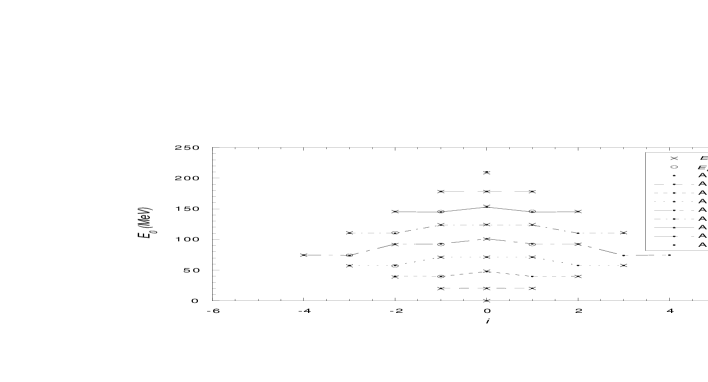
Figure 1: Coulomb corrected $0^{+}$ state energy $E_{0}$ vs. the isospin projection $i$ for the isotopes of nuclei with $Z=20$ to $Z=28$ in the $1f_{7/2}$ level, $\Omega_{7/2}=4.$ The experimental binding energies $E_{BE}^{\exp}$ (symbol “$\times$”) are distinguished from the experimental energies of the isobaric analog $0^{+}$ excited states $E_{exc}^{\exp}$ (symbol “$\circ$”). Each line connects theoretically predicted energies of an isobar sequence. The nuclei for which experimental data is not available are represented only by their predicted $0^{+}$ state energy.

An observation about the $pn$-pairing strength is that most of $pn$-coupling study has been done assuming good isospin, that is $F=G$. However, the free nucleon-nucleon data [59] indicates that the $\tau=1\ pn$-pairing strength ($G$) is slightly bigger than the like-particle pairing strength ($F$), which is confirmed by the fits presented in Table 3 and is investigated in other studies [27, 60]. There are many different values for the like-particle pairing strength used in literature. The most common value is taken to be proportional to $1/A$ [5, 10, 61, 62, 63] and is consistent with the experimental pairing gaps derived from the odd-even mass differences [64, 65]. The values of $F$, obtained by our theoretical symplectic model, fall within the limits of their estimation. In this way, they are expected to reproduce the low-lying vibrational spectra of spherical nuclei in the $SU^{\pm}(2)$ limit. When the results from all the three non-deformed fits are considered (Table 3), the identical-particle parameter $F/\Omega$ is found to decrease with the mass number as $23.\,9/A$. In a similar way, one can find the dependence of the $pn$ pairing strength parameter $G/\Omega$ on the mass number to be $25.\,7/A$.

The estimate of the parameters (Table 3) reveals the properties of the nuclear interaction as interpreted by connection (9). The $J=0$ pairing interaction ($V_{P_{0}}$) is always attractive, while the overall high-$J$ component of identical-nucleon coupling $\left\langle\pm\pm\left|V\right|\pm\pm\right\rangle$ might be repulsive. The $J>0$ proton-neutron “direct” interaction $\left\langle-+\left|V\right|-+\right\rangle$ is attractive, but not the “exchange” part of it $\left\langle-+\left|V\right|+-\right\rangle$ ($E<0$).

In all cases there is a good agreement with experiment (small $\chi$), as can be seen in Table 3, as well as in Figure 1 for region $({\bf II}).$ Part of our results, namely for the binding energies (but not for the excited $0^{+}$ state energies), can be compared to other theories. A direct comparison of the chi statistics is impossible because of the different data sets and energy levels determined by the various theories. However, if we select only the data subsets that are equivalent for the nuclei in the $1d_{3/2}$ and/or $1f_{7/2}$, our results are much closer to the experimental numbers than those for the Hartree-Fock-Bogoliubov ($HFB$) model [43] and the semi-empirical model [44] and comparable with those of the $jj$-coupling shell model [13, 42] and the isovector and isoscalar pairing plus quadrupole model [37]. In this way the simple $Sp(4)$ model is tested and proves its validity when applied to light nuclei in single-$j$ level. In this region many symmetries are conserved allowing for a possible reduction of the number of fitting parameters. However, the free parameters in the fits presented in Table 3 reflect the symmetries observed in light nuclei and the non-negligible symmetry breaking in medium-mass nuclei.

Properties of the pairing interaction – A model with the $Sp(4)$ dynamical symmetry permits an independent investigation of the different kinds of pairing interactions in the limiting cases of the non-deformed (18), (19) as well as the deformed versions (20), (21) of the theory. In the $SU^{\pm}(2)$ limit, the symplectic model reproduces the properties of the identical-nucleon pairing ($\varepsilon_{pp}+\varepsilon_{nn}$) (19), for which the usual parabolic dependence of $\varepsilon_{pp(nn)}$ on $N_{\pm}$ holds [10, 9, 13, 38]. The dependence of the like-particle energy on the isospin projection $i$ (Figure 2(a)) reveals another property of the pairing mode, a $\triangle i=1$ staggering of the identical-nucleons pairing energies of the odd-odd and even-even nuclei.

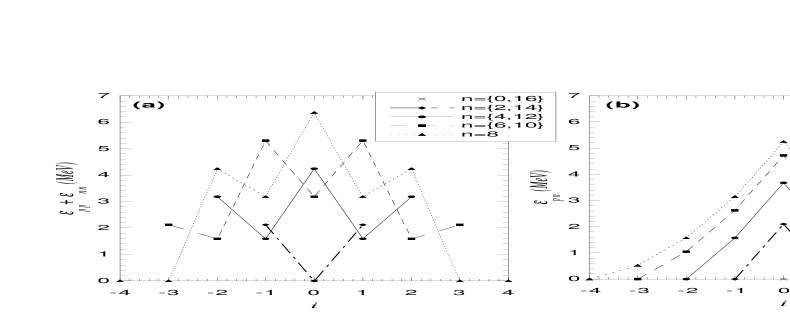
Figure 2: Identical ($G=0,\ F=1.81$ (a)) and non-identical ($G=2.10,\ F=0$ (b)) particle pairing energies vs. $i$ for isobars with $A=40$ to $A=56$ in the $1f_{7/2}$ level

In contrast with this, the $pn$ limit ($\varepsilon_{pn}$) shows a smooth behavior (Figure 2 (b)). The $SU^{0}(2)$ limiting case yields a proton-neutron coupling that has its maximum when $N_{+}=N_{-}$ ($i=0$), which is consistent with $\alpha-$clustering theories [66, 67] and the charge independence in the region of light nuclei when protons and neutrons fill the same shell [32, 34]. In both limits ($SU^{\pm}(2)$ and $SU^{0}(2)$ ), the pairing energy decreases when the difference between proton and neutron numbers increases.

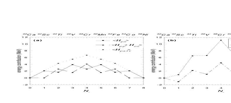
Figure 3: Lowest isovector-paired $0^{+}$ state energies vs. $N_{-}$ when $N_{+}=N_{-}$ for the nuclei in $1f_{7/2}$: (a) pairing energies: $pn,$ $pp+nn$ and total; (b) symmetry energy ($E$ term in (6)) and total pairing + symmetry energy

In most nuclei the different pairing interactions coexist and the contribution of each of the pairing modes, $\left\langle H_{pp}+H_{nn}\right\rangle$ $=$ $F\left\langle A_{+1}B_{+1}+A_{-1}B_{-1}\right\rangle$ and $\left\langle H_{pn}\right\rangle=G\left\langle A_{0}B_{0}\right\rangle$, to the total pairing energy $\left\langle H_{pair}\right\rangle=\left\langle H_{pn}\right\rangle+\left\langle H_{pp}+H_{nn}\right\rangle$ can be investigated. A $\triangle N=2$ staggering exists for both pairing interactions (Figure 3(a)) [22, 68, 31]. For $N_{+}=N_{-}$ odd-odd nuclei the $\tau=1\ pn$ pairs give the dominant contribution, while for the even-even $N_{+}=N_{-}$ nuclei both pairing modes contribute almost equally with a slightly greater like-particle contribution. Although difference between even-even and odd-odd nuclei exists in each pairing contribution, the total pairing energy has a surprisingly smooth behavior. The contribution from the symmetry term ($E$ term in (6)) [24, 34] restores the staggering, as it decreases the energy of the odd-odd nuclei with respect to their even-even neighbors (Figure 3(b)).

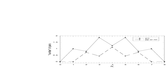
Figure 4: Non-identical ($pn$) and identical ($pp$ or $nn$) pairing “numbers” vs. $N_{-}$ for the $N_{+}=N_{-}$ nuclei with $Z=20$ to $Z=28$ in $1f_{7/2}$

Rough measures for the number of $pn$ and like-particle pairs are the quantities $\frac{1}{G}\left\langle H_{pn}\right\rangle$ and $\frac{1}{F}\left\langle H_{pp}+H_{nn}\right\rangle$, respectively, which are related to the pairing gaps [22, 23]. The “number” of $pn$ pairs (Figure 4) is bigger than the “number” of $pp(nn)$ pairs for odd-odd $N_{+}=N_{-}$ nuclei, and is of the same order as for the even-even nuclei [22, 68, 31].

Deformed non-linear model – To investigate the role of the $q$-deformation, we performed again the fitting procedures for the same regions (${\bf(I)}$, ${\bf(II)}$ and ${\bf(III)}$) but using the deformed Hamiltonian (17). For each group of nuclei, the outcome of a fit with all possible parameters ($G_{q},\ F_{q},\ E_{q},\ C_{q},\ D_{q},\ \epsilon^{q}$ and $q$) indicates that the introduction of the $q$-deformation does not vary the rest of the parameters. Based on this result, we considered the deformation to be independent of the other parameters and varied only $q$ in the fit (the rest of the parameters were kept fixed with values obtained from the non-deformed fit). The results are shown in the “$q$-def” columns in Table 3. The fits with and without a deformation can be compared by using the residual sum of squares ($S$), which is always smaller in the deformed case (Table 3).

Although it stands in contrast with other $q$-deformed applications [40, 41], the decoupling of the $q$-deformation from the interaction strengths is not an assumption but results from comparisons to experimental data over total of $149$ nuclei. It implies that while leaving the strength of the two-body interactions unchanged, the $q$-deformation allows one to take into account, in a prescribed way, complicated dependence of the energy eigenvalues on the number of nucleons/pairs and space dimension that cannot be reproduced by any two-body interaction (for example, see (20) and (21)). Moreover, similar terms are expected to arise from higher-order interactions between the particles. In this way the $q$-parameter introduces some non-linear residual interaction not present in the two-body Hamiltonian (6).

The observed independence of the pairing strengths on the $q$-parameter, suggests that while the deformation does not change the strength to couple two particles, it can model many-pair effects and can influence the energy spectrum. As an illustration, in each of the dynamical limits we investigate the quantities $R_{pn}=\varepsilon_{pn}^{q}/\varepsilon_{pn}$ and $R_{pp+nn}=(\varepsilon_{pp}^{q}+\varepsilon_{nn}^{q})/(\varepsilon_{pp}+\varepsilon_{nn})$ that give an additional contribution to the pairing energy in the deformed case (Figure 5) (compare to the analytical expansion with respect to $\varkappa$ of the energies, (20) and (21)). In the limit of $pn$-pairing, $R_{pn}$ does not significantly change when $q$ is close to one and it decreases for all $q\neq 1$. The ratio $R_{pp+nn}$ increases (decreases) monotonically with $q$ only for nuclei with a primary $pp$ ($nn$) coupling. Even though both $SU_{q}^{\pm}(2)$ groups are complementary, the different behavior of the multiplication constants $\rho_{\pm}$ (Table 1) is responsible for different impact of the deformation in various isotopes. This accounts for the differences in the experimental data between mirror nuclei even after the Coulomb energy correction. In the limit of identical-particle coupling, when $q$ increases from one ($q>1$) neutron pairs are less bound and proton pairs give a larger pairing gap, and vice versa for $q<1$. In this way, the deformation parameter can determine the degree to which the $pp$ coupling differs from the $nn$ coupling.

The significance of the higher-order terms that enter through the $q$-deformed theory can be estimated through a comparison with experiment. In general, the fitting procedures determine values for $\varkappa$ (Table 3) that are small. The reason may be that while higher-order effects may be significant in nuclei they probably cancel on average when the $q$-parameter is one and the same for all nuclei. However, in two of the cases, $({\bf II})$ and $({\bf III})$, it is of an order of magnitude greater than the estimation of other physical applications ([39] and references there) and for the shell $1f_{7/2}$, our value ($q=1.\,132$) is comparable to the values obtained in a $q$-deformed like-particle seniority model [40]: $q=1.\,1585$ for the neutron pairs and $q=1.\,1924$ for protons. For the nuclei in the multi-$j$ shell our model yields a bigger $q$-parameter than for the lighter nuclei in single-$j$ shell (Table 3), where the small number of valence nucleons is not sufficient to build strong non-linear correlations. This suggests that the $q$-deformation is more significant for masses $A>56$.

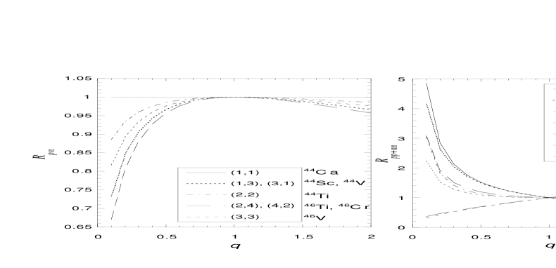
Figure 5: Ratios $R_{pn}$ and $R_{pp+nn}$ vs. $q$ for several nuclei with a typical behavior in the $1f_{7/2}$ level

4.2 Predicted energies

The fitting procedure not only estimates the magnitude of the pairing strength and describes the type of the dominant coupling mode, it also can be used to predict nuclear energies that have not been measured. From the fit for the $1f_{7/2}$ case the binding energy of the proton-rich ${}^{48}Ni$ nucleus is estimated to be $348.19$ MeV, which is by $0.07\%$ greater than the sophisticated semi-empirical estimate of [44]. Likewise, for the odd-odd nuclei that do not have measured energy spectra the theory can predict the energy of their lowest $0^{+}$ isobaric analog state: $358.75$ MeV (${}^{44}V$), $359.49$ MeV (${}^{46}Mn$), $357.56$ MeV (${}^{48}Co$), $394.16$ MeV (${}^{50}Co$). The predicted energies are calculated for $q=1.132$ (Table 3 (II)) as the fit with deformation has a smaller uncertainty compared to the non-deformed one. The $Sp_{(q)}$ model predicts the relevant $0^{+}$ state energies for additional 165 even-$A$ nuclei in the medium mass region (III). The binding energies for 25 of them are also calculated in [44]. For these even-even nuclei, we predict binding energies that on average are by $0.05\%$ (non-deformed case) and by $0.008\%$ (for $q=1.240$) less than the semi-empirical approximation [44].

5 Conclusion

We constructed a model with a symplectic dynamical symmetry group $Sp_{(q)}(4)\supset U(1)\otimes SU_{(q)}(2)$ in the non-deformed limit as well as in the $q$-deformed generalization. A phenomenological Hamiltonian was written in terms of the generators of the group and this in turn was used to describe pairing correlations in nuclei. The relation of this approach to a general microscopic pairing Hamiltonian was obtained. The theory was tested by fitting calculated energies to the relevant experimental $0^{+}$ state energies for single-$j$ levels, namely $1d_{3/2}$ and $1f_{7/2}$, and for a multi-$j$ $1f_{5/2}2p_{1/2}2p_{3/2}1g_{9/2}$ shell. In general, the fitting procedure yielded results that were in good agreement with the experiment. The theory predicted the lowest $0^{+}$ isovector-paired state energy of nuclei with a deviation of at most $0.5\%$ in the energy range considered. It was used to predict the binding energy for even-even nuclei and the lowest isovector-paired $0^{+}$ state energy of odd-odd nuclei in the proton-rich region. The phenomenological pairing parameters and the strength of the pairing interaction were determined. In agreement with experimental analysis, breaking of the isospin invariance, $\eta_{2}/\eta_{1}\neq 0$, and isospin mixing, $G>F$, is observed, except for light nuclei in the $1d_{3/2}$ level.

The theoretical model with $Sp(4)$ dynamical symmetry and its $q$-deformed version was used to investigate in greater detail the properties of the isovector pairing interaction. The study reveals that the pairing energy along with the symmetry energy are responsible for the experimentally observed staggering between even-even and odd-odd nuclear isovector-paired $0^{+}$ state energies. Overall, the results show that the symplectic model can be used to provide a reasonable description of isovector-paired $0^{+}$ states in nuclei, confirming in its limit results previously published for like-particle pairing correlations. When only the nuclei with $0^{+}$ ground states are considered, the non-deformed $Sp(4)$ model is comparable, for the region of light nuclei, to earlier theories. At the same time it gives some insight into the study of symmetry breaking and isovector pairing correlations, and it is based on a simple approach that is applicable in a broad region of the nuclear chart, including odd-odd and exotic nuclei.

The $q$-deformed case gives the best overall results. The $Sp_{q}(4)$ dynamical symmetry approach yielded a $q$-deformed exact solution and we were able to derive the $q$-deformed matrix elements of the interaction in a simple analytical form. In addition to the broken symmetries of the non-deformed model, the $q$-deformation breaks the symmetry between protons and neutrons, which again is small for light nuclei and consistent with experiment. The introduction of $q$ leads to a decrease of the like-particle pairing gap for neutrons and an increase for protons as $q$ increases from one. The $q$-parameter was found decoupled from the interaction strength parameters. This observation suggests that while the deformation does not influence the two-body interaction, it introduces higher-order interactions between the particles, which are neglected in most non-deformed models. The $q$-deformation is mass and shell dimension dependent and its effects are more significant in the medium mass region. In the present study, the $q$-parameter was found as high as $1.240$ and is expected to be greater if its influence is not averaged over all nuclei in a major shell. This suggests the need for a more elaborate investigation of the role of the $q$-deformation in each individual nucleus and the relation of the $q$-parameter to the underlying nuclear structure.

This work was supported by the US National Science Foundation, Grant Numbers 9970769 and 0140300. The authors appreciate the encouraging discussions of this work with Professor Feng Pan, Dr. Chairul Bahri and Dr. Carl E. Svensson, as well as with Dr. Vesselin G. Gueorguiev, whom we thank also for his computational MATHEMATICA programs for non-commutative algebras.

References

- [1] G. Racah, Phys. Rev. 62, 438 (1942), Phys. Rev. 63, 367 (1943).
- [2] B. H. Flowers, Proc. Roy. Soc. (London) A212, 248 (1952).
- [3] A. Bohr, B. R. Mottelson, D. Pines, Phys. Rev. 110, 936 (1958); S. T. Belyaev, Mat. Fys. Medd. 31, 11 (1959).
- [4] A. de-Shalit, I. Talmi, Nuclear Shell Theory, Academic Press, New York (1963).
- [5] A. M. Lane, Nuclear Theory, W. A. Benjamin, Inc. (1964).
- [6] K. Langanke, Nucl. Phys. A630, 368c (1998).
- [7] H. Schatz et. al, Phys. Rep.294, 167 (1998).
- [8] A. L. Goodman, Adv. Nucl. Phys. 11, 263 (1979).
- [9] A. K. Kerman, Ann. Phys., NY 12, 300 (1961).
- [10] A. K. Kerman, R. D. Lawson, M. H. Macfarlane, Phys. Rev. 124, 162 (1961).
- [11] F. Pan, J. P. Draayer, W. E. Ormand, Phys. Lett. B422, 1 (1998); F. Pan, J. P. Draayer, Phys. Lett. B442, 1 (1998).
- [12] K. Helmers, Nucl. Phys. 23, 594 (1961).
- [13] I. Talmi, SimpleModels of Complex Nuclei: The Shell Model and Interacting Boson Model, Harwood Academic Publishers GmbH, Switzerland (1993).
- [14] K. T. Hecht, Nucl. Phys. 63 , 177(1965), Phys. Rev. 139, B794 (1965), Nucl. Phys. A102, 11 (1967).
- [15] J. N. Ginocchio, Nucl. Phys. 74, 321 (1965).
- [16] J. C. Parikh, Nucl. Phys. 63, 214 (1965).
- [17] G. G. Dussel et. al., Nucl. Phys. A153, 469 (1970).
- [18] S. C. Pang, Nucl. Phys. A128, 497(1969).
- [19] J. Engel, S. Pittel, M. Stoitsov, P. Vogel, J. Dukelsky, Phys. Rev. C55, 1781 (1997).
- [20] Yu.V. Palchikov, J. Dobes, R.V. Jolos Phys. Rev. C 63, 034320 (2001).
- [21] P. Van Isacker, D. D. Warner, Phys. Rev. Lett. 78, 3266 (1997).
- [22] J. Engel, K. Langanke, P. Vogel, Phys. Lett. B389, 211 (1996).
- [23] J. Dobes, Phys. Lett. B413, 239 (1997).
- [24] N. Zeldes, S. Lirin, Phys. Lett. 62B, 12 (1976).
- [25] D. Rudolph , Phys. Rev. Lett. 76, 376 (1996).
- [26] J. Garces Narro , Phys. Rev. C63, 044307 (2001).
- [27] O. Civitarese, M. Reboiro, P. Vogel, Phys. Rev. C56, 1840 (1997).
- [28] K. Langanke, D. J. Dean, S. E. Koonin, P. B. Radha, Nucl. Phys. A613, 253 (1997); D. J. Dean, S. E. Koonin, K. Langanke,P. B. Radha, Phys. Lett. B399, 1 (1997).
- [29] A. Poves, G. Martinez-Pinedo, Phys. Lett. B430, 203 (1998).
- [30] G. Martinez-Pinedo, K. Langanke, P. Vogel, Nucl. Phys. A651, 379 (1999).
- [31] K. Kaneko, M. Hasegawa, J. Zhang Phys. Rev. C59, 740 (1999).
- [32] A. O. Macchiaveli et. al., Phys. Lett. B480, 1 (2000).
- [33] A. O. Macchiaveli et. al., Phys. Rev. C61, 041303(R) (2000).
- [34] P. Vogel, Nucl. Phys. A662, 148 (2000).
- [35] W. Satula, R. Wyss, Phys. Lett.B393, 1 (1997); Nucl. Phys. A676, 120 (2000).
- [36] W. Satula, D.J. Dean, J. Gary, S. Mizutori, W. Nazarewicz Phys. Lett.B407, 103 (1997).
- [37] M. Hasegawa, K. Kaneko, Phys. Rev. C59, 1449 (1999).
- [38] K. L. G. Heyde, The Nuclear Shell Model, Springer Series in Nuclear and Particle Physics (1990); W. Greiner, J. A. Maruhn, Nuclear Models, Springer-Verlag Berlin Heidelberg (1996).
- [39] D. Bonatsos, J. Phys. A: Math. Gen. 25, L101 (1992).
- [40] S. Shelly Sharma, Phys. Rev. C46, 904 (1992).
- [41] S. Shelly Sharma, N. K. Sharma, Phys. Rev. C50 , 2323 (1994); Phys. Rev. C62 , 034314 (2000).
- [42] I. Talmi, R. Thieberger, Phys. Rev. 103, 718 (1956).
- [43] T. S. Sandhu, M. L. Rustgi, Phys. Rev. C12 , 666 (1975).
- [44] P. Möller, J. R. Nix, K.-L. Kratz, LA-UR-94-3898 (1994); At. Data Nucl. Data Tables 66, 131 (1997).
- [45] K. D. Sviratcheva, A. I. Georgieva, V. G. Gueorguiev, J. P. Draayer, M. I. Ivanov, J. Phys. A: Math. Gen. 34, 8365 (2001).
- [46] A. Klein, E. Marshalek, Rev. Mod. Phys. 63 , 375 (1991).
- [47] S. Szpikowski, W. Berej, L. Prochniak, Symmetries in Science X, Plenum Press (1997).
- [48] E. Hagberg et. al., Phys. Rev. Lett. 73, 396 (1994).
- [49] W. E. Ormand, B. A. Brown, Phys. Rev. C52, 2455 (1995).
- [50] A. F. Lisetskiy et. al, Phys. Rev. Lett. 89, 012502 (2002).
- [51] J. Jänecke, H. Behrens, Phys. Rev. C9, 1276 (1974).
- [52] J. Duflo, A. P. Zuker, Phys. Rev. C52, R23 (1995).
- [53] S. Goshen and H. J. Lipkin, Spectroscopic and group theoretical methods in physics, Amsterdam: North-Holland (1968).
- [54] K. Kaneko, M. Hasegawa, Phys. Rev. C60, 024301 (1999).
- [55] P. Van Isacker, Rep. Prog. Phys. 62, 1661 (1999).
- [56] G. Audi, A. H. Wapstra, Nucl. Phys. A595, 409 (1995).
- [57] R. B. Firestone, C. M. Baglin, Table of Isotopes (8th Edition) , John Wiley & Sons (1998).
- [58] J. Retamosa, E. Caurier, F. Nowacki, A. Poves, Phys. Rev. C55, 1266 (1997).
- [59] R. D. Lawson, Phys. Rev. C19, 2359 (1979).
- [60] H. T. Chen, A. Goswami, Nucl. Phys. 88, 208 (1966).
- [61] L. S. Kisslinger, R. A. Sorensen, Rev. Mod. Phys. 35, 853 (1963).
- [62] A. Bohr, B.R. Mottelson, Nuclear Structure (Benjamin, New York, 1969).
- [63] J. Dudek, A. Majhofer, J. Skalski, J. Phys. G 6, 447 (1980).
- [64] S. G. Nilsson, O. Prior, Mat. Fys. Medd. Dan. Vid. Selsk. 32, No.16 (1961).
- [65] P. Ring, P. Schuck, The Nuclear Many-Body Problem (Springer-Verlag New York Inc., 1980).
- [66] M. Hasegawa, K. Kaneko, Phys. Rev. C61, 037306 (2000); Y. K. Gambhir, P. Ring, P. Schuck, Phys. Rev. Lett. 51, 1235 (1983).
- [67] G. Röpke, A. Schnell, P. Schuck, P. Nozieres, Phys. Rev. Lett. 80, 3177 (1998); G. Röpke, A. Schnell, P. Schuck, U. Lombardo, Phys. Rev. C61, 024306 (2000).
- [68] K. Langanke, Nucl. Phys. A613, 253 (1997).