Effect of transients in nuclear fission on multiplicity of prescission neutrons

Abstract

Transients in the fission of highly excited nuclei are studied in the framework of the Langevin equation. Time-dependent fission widths are calculated which show that a steady flow towards the scission point is established, after the initial transients, not only for nuclei which have fission barriers but also for nuclei which have no fission barrier. It is shown from a comparison of the transient time and the fission life time that fission changes from a diffusive to a transient dominated process over a certain transition region as a function of the spin of the fissioning nucleus. Multiplicities of prescission neutrons are calculated in a statistical model with as well as without a single swoop description of fission and they are found to differ in the transition region. We however find that the difference is marginal and hence a single swoop picture of fission though not strictly valid in the transition region can still be used in the statistical model calculations.

1 Introduction

The fission dynamics of hot compound nuclei continues to be a subject of considerable interest essentially due to the fact that the fission life time determined from the phase space argument of Bohr and Wheeler turns out to be too small to allow for the rather large number of experimentally observed light particles evaporated prior to fission [1]. It was therefore felt necessary to look beyond the statistical model and this gave rise to a revival of interest in the original work of Kramers who considered fission as a diffusive probability flow over the fission barrier [2]. Dissipative dynamical models of fission were subsequently developed to include particle emission and were found to reproduce a host of experimental data [3, 4, 5].

In a dissipative dynamical model, the dynamics associated with the fission degree of freedom is usually considered to be similar to that of a Brownian particle floating in a viscous heat bath. The heat bath in this picture represents the rest of all the other nuclear degrees of freedom which are assumed to be in thermal equilibrium. The interaction between these large number of intrinsic degrees of freedom and the fission degree of freedom gives rise to a random force and consequently a dissipative drag on the dynamics of fission [4]. The fission trajectory can thus be followed by solving the appropriate Langevin equation [4, 5]. Alternatively, one can study the time evolution of the phase space density of the fission coordinates using the Fokker-Planck equation [3, 6].

Several time scales are of physical significance as a compound nucleus makes its journey from its formation to its scission. Considering an ensemble of compound nuclei which are all formed at a given instant, it requires a certain interval of time in order to develop a steady probability flow at the saddle point across the fission barrier. During this time interval, also referred to as the transient time ($\tau$) [7, 8], the probability flow at the saddle point increases from zero to its statioanry value. This stationary probability flow also defines the stationary fission width ($\Gamma_{0}$) and the associated fission life time ($\tau_{f}=\hbar/\Gamma_{0}$). However, the entire fission process itself becomes a transient when the compound nucleus has no fission barrier. In such cases, it is usually argued that the full distribution reaches the scission point in a single swoop [7]. The compound nucleus then survives exactly the swooping down time ($\tau_{s}$) in this picture. These transients in nuclear fission were considered earlier in great details in a series of publications [7, 8, 9]. Using a number of simplifying assumptions, analytical expressions were obtained for the time dependent fission widths for both the weakly damped and strongly damped motions [8, 9]. The stationary value of the fission width was obtained by Kramers earlier [2]. The transient time for cases where there is no barrier was also obtained [7].

An highly excited nucleus can emit a number of light particles (including photons) before it undergoes fission. In order to trace the time evolution of such a hot nucleus, it would therefore be most desirable to couple a dynamic theory of fission with the statistical emission of light particles. Extensive work has been done in this direction using either the Fokker-Planck or the Langevin equations and the importance of the dynamic nature of the fission process at high excitations has been established [3, 4, 5]. Such calculations however are quite involved and require a large computer time. An alternative and easier approach would be to perform a statistical model calculation by modifying a cascade code in which fission is treated as one of the decay channels and the time dependence of the fission width is explicitly taken into account [10]. In such calculations, the input fission widths and the transient times are usually taken from the analytical expressions [2, 3, 6].

In the present work, we would examine certain issues related to the time dependence of fission widths and its effect on the multiplicity of the prescission neutrons. First, we would study the effect of lowering the fission barrier on the time dependence of the rate of fission. We would use the Langevin equation to model the fission dynamics for our purpose. The motivation for this study is to find the transition from a diffusive process in the presence of a fission barrier to a transient dominated picture when there is no fission barrier. We would indeed find that the diffusive nature of fission continues to some extent even for cases which have no fission barrier. The underlying physical picture that would emerge for fission in the absence of a fission barrier would be as follows. Consider an ensemble of fission trajectories which have started together sliding down the potential (with no fission barrier) towards the scission point. However, the random force acting on the trajectories will introduce a dispersion in their arrival time at the scission point. In other words, the trajectories will cross the scission point at different instants and a flow will thus be established at the scission point. However, the effect of this dispersion will be reduced when the conservative force becomes much stronger than the random force. This would happen at very large angular momentum of the fissioning nucleus due to the strong centrifugal force. Therefore, the single swoop picture for fission becomes more appropriate at very large values of spin of the nucleus. We would establish the above scenario in the first part of our work.

Next, we would perform statistical model calculations for prescission neutron multiplicity using the time dependent fission widths as well as the single swoop description of fission. This would be done with the aim of finding how well the statistical model calculations with and without the single swoop assumption agree with each other. We would subsequently calculate the prescission neutron multiplicity in a dynamical model of fission and would compare the results with those obtained from the statistical calculations. Though one would expect the results from the statistical and the dynamical calculations to be the same, there could be some differences due to reasons such as the following one. The neutron width at any instant of time evolution of a hot nucleus depends upon its temperature. However, a part of the total excitation energy is used to build up the collective kinetic energy in the fission channel in the dynamical model. This reduces the available intrinsic excitation energy, and hence the temperature, in the dynamical model compared to the statistical model calculation where the total excitation energy is taken as the intrinsic excitation energy of the nucleus. This could reduce the neutron multiplicity in a dynamical model than that obtained from a statistical calculation. We would ascertain the magnitude of such differences from our calculation.

The time dependent fission widths will be evaluated by solving the Langevin equation numerically in the present paper. We have to resort to numerical methods rather than using analytical solutions due to the fact that analytical solutions assume a constant friction whereas we would use a strongly shape dependent friction force in our calculation. This shape dependent friction is a modified version of the one-body wall friction, the so-called ”chaos-weighted wall formula”, in which the effect of chaos in the single-particle motion is incorporated [11]. The prescission neutron multiplicity and fission probability calculated from Langevin dynamics using the chaos-weighted wall friction were found to agree fairly well with the experimental data for a number of heavy compound nuclei ($A\sim 200$) over a wide range of excitation energies [12]. Since the chaos-weighted wall friction contains no adjustable parameter to fit the experimental data, we consider this to be the most appropriate dissipative force to describe the dynamics of fission and accordingly we shall use it here. Further, we have already reported a systematic study of fission widths using this friction [13]. This study was confined to cases with fission barriers whereas we would concentrate upon fission in the absence of a barrier in the present work.

We shall give a brief description of the dynamical model for fission in the next section. Section 3 will contain the numerical results. A summary of the results along with the conclusions will be presented in the last section.


2 Langevin dynamics of fission

2.1 Nuclear shape, potential and inertia

We shall choose the shape parameters $c,h$ and $\alpha$ as suggested by Brack et al. [14] as the collective coordinates for the fission degree of freedom. However, we will simplify the calculation by considering only symmetric fission ($\alpha=0$). We shall further assume in the present work that fission would proceed along the valley of the potential landscape in $(c,h)$ coordinates though we shall consider the Langevin equation in elongation $(c)$ coordinate alone in order to simplify the computation. Consequently, the one-dimensional potential in the Langevin equation will be defined as $V(c)=V(c,h)$ at valley and the coupled Langevin equations in one dimension will be given [15] as

$$\frac{dp}{dt} = -\frac{p^{2}}{2}\frac{\partial}{\partial c}\left({1\over m}\right)-\frac{\partial F}{\partial c}-\eta\dot{c}+R(t),$$ (1)

$$\frac{dc}{dt} = \frac{p}{m}.$$ (2)

The shape-dependent collective inertia and the friction coefficient in the above equations are denoted by $m$ and $\eta$ respectively. The free energy of the system is denoted by $F$ while $R(t)$ represents the random part of the interaction between the fission degree of freedom and the rest of the nuclear degrees of freedom considered collectively as a thermal bath in the present picture. The collective inertia, $m$, will be obtained by assuming an incompressible irrotational flow and making the Werner-Wheeler approximation [16]. The driving force in a thermodynamic system should be derived from its free energy which we will calculate considering the nucleus as a noninteracting Fermi gas [17]. The instantaneous random force $R(t)$ is modeled after that of a typical Brownian motion and is assumed to have a stochastic nature with a Gaussian distribution whose average is zero [4]. The strength of the random force will be determined by the friction coefficient through the fluctuation-dissipation theorem. A detailed description of the various input quantities may be found in a recent publication [13].


2.2 Nuclear friction

In order to define the friction force in the Langevin equation (eq.(1)), we will consider the one-body wall and window dissipation [18]. We will use the chaos-weighted wall friction as the one-body wall dissipation. We shall give here a brief description of the chaos-weighted wall friction, the details of which is given elsewhere [11]. The chaos-weighted friction coefficient ${\eta_{cwwf}}$ is given as

$$\eta_{cwwf}=\mu\eta_{wf},$$ (3)

where ${\eta_{wf}}$ is the friction coefficient as was given by the original wall formula [18] and ${\mu}$ is a measure of chaos (chaoticity) in the single-particle motion of the nucleons within the nuclear volume and depends on the instantaneous shape of the nucleus [11]. In the present classical picture, this will be given as the average fraction of the nucleon trajectories that are chaotic when the sampling is done uniformly over the nuclear surface. The value of chaoticity is evaluated for a given shape of the nucleus by sampling over a large number of classical nucleon trajectories while each trajectory is identified either as a regular or as a chaotic one by considering the magnitude of its Lyapunov exponent and the nature of its variation with time [19]. It is observed that the value of chaoticity $\mu$ changes from 0 to 1 as the nucleus evolves from a spherical shape to a highly deformed one. This implies that the wall friction is very small for near spherical shapes of a nucleus. The physical picture behind this is as follows. A particle moving in a spherical mean field represents a typical integrable system and its dynamics is completely regular. When the boundary of the mean field is set into motion (as in fission), the energy gained by the particle at one instant as a result of a collision with the moving boundary is eventually fed back to the boundary motion in the course of later collisions [20]. An integrable system thus becomes completely nondissipative resulting in a vanishing friction coefficient. On the other hand, the nucleon motion becomes chaotic in a highly deformed nucleus. Consequently, the energy tranfer from boundary motion to particle motion becomes irreversible giving rise to a large friction force acting on the boundary motion. These aspects were established from various numerical investigations [21, 22] and was incorporated into the wall formula to give the chaos-weighted wall friction [11].

In the wall and window model of one-body dissipation, the window friction is expected to be effective after a neck is formed in the nuclear system [23]. Further, the radius of the neck connecting the two future fragments should be sufficiently narrow in order to enable a particle that has crossed the window from one side to the other to remain within the other fragment for a sufficiently long time. This is necessary to allow the particle to undergo a sufficient number of collisions within the other side and make the energy transfer irreversible. It therefore appears that the window friction should be very nominal when neck formation just begins. Its strength should increase as the neck becomes narrower reaching its classical value when the neck radius becomes much smaller than the typical radii of the fragments. We however know very little regarding the detailed nature of such a transition. We shall therefore refrain from making any further assumption regarding the onset of window friction. Instead, we shall define a transition point in the elongation coordinate $c_{win}$ beyond which the window friction will be switched on. We shall also assume that the compound nucleus evolves into a binary system beyond $c_{win}$ and accordingly correction terms for the motions of the centers of mass of the two halves will be applied to the wall formula for $c>c_{win}$ [23]. However, it may be noted that while the window friction makes a positive contribution to the total friction, the centre of mass motion correction reduces the wall friction. The two contributions therefore cancel each other to some extent. Consequently, the resulting wall-and-window friction is not very sensitive to the choice of the transition point. We shall choose a value for $c_{win}$ at which the nucleus has a binary shape and the neck radius is half of the radius of either of the would-be fragments.

The chaos weighted wall and window friction will thus be given as

$$\eta(c<c_{win})=\eta_{cwwf}(c<c_{win}),$$ (4)

and

$$\eta(c\geq c_{win})=\eta_{cwwf}(c\geq c_{win})+\eta_{win}(c\geq c_{win}).$$ (5)

The detailed expressions for the wall and window frictions can be found in ref. [23].


3 Results

3.1 Fission widths from Langevin equation

With all the necessary input defined as above, the Langevin equation (eq.(1)) is numerically integrated following the procedure outlined in ref.[4]. Starting with a given total excitation energy ($E^{*}$) and angular momentum ($l$) of the compound nucleus, the energy conservation in the following form,

$$E^{*}=E_{int}+V(c)+p^{2}/2m$$ (6)

gives the intrinsic excitation energy $E_{int}$ and the corresponding nuclear temperature $T=(E_{int}/a)^{1/2}$ at each integration step. A Langevin trajectory will be considered as having undergone fission if it reaches the scission point ($c_{sci}$) in the course of its time evolution. The calculations are repeated for a large number (typically 100 000 or more) of trajectories and the number of fission events is recorded as a function of time. Subsequently the time dependent fission rates can be easily evaluated.

We have chosen the ²⁰⁰Pb compound nucleus for our study which has been experimentally formed at differnt excitation energies in a number of heavy ion induced fusion reactions [24, 25, 26]. Figure 1 shows the calculated time dependent fission widths at different spins of the compound nucleus for a given temperature. A number of interesting observations can be made from this figure. The time dependence of the fission width of the compound nucleus with a spin of 40$\hbar$ (and with a fission barrier) is typical of a diffusive flow across the fission barrier which has been studied extensively on an earlier occasion [13]. The fission width is found to remain practically zero till a certain interval of time ($t_{0}$) which essentially corresponds to the interval after which the fission trajectories start arriving at the scission point. The fission width subsequently increases with time till it reaches its stationary value ($\Gamma_{0}$). We will use the following parametric form for the time dependent fission width in order to enable us to use it in our later calculations,

$$\Gamma(t)=\Gamma_{0}[1-exp(-(t-t_{0})/\tau)]\Theta(t-t_{0})$$ (7)

where $\tau$ is a measure of the transient time after which the stationary flow is established and $\Theta(t)$ is the step function. The intervals $t_{0}$ and $\tau$ are obtained by fitting the calculated fission widths with the above expression.

We next note in fig. 1 that the nature of the time dependence of the fission width remains almost same even though the fission barrier decreases and subsequently vanishes with increasing spin. At very large values of spin, however, fluctuations appear at the later stages of time evolution. These fluctuations are statistical in nature because the number of nuclei which have not yet undergone fission decreases very fast with increasing time for higher values of spin and therefore introduces large statistical errors in the measured numbers. The magnitude of the fluctuations can thus be reduced by considering a larger number of fission trajectories. In our calculation, we have taken particular care by using larger ensembles at higher values of nuclear spin in order to enable us to check whether a stationary value of the fission width is attained at all.

The above observation is of particular interest since it shows that the diffusive nature of fission persists even for cases which have no fission barrier. This diffusive nature is a consequence of the random force acting on the fission trajectories as we have discussed earlier. As a compound nucleus is formed having no potential pocket in the fission channel, it starts rolling down the potential towards the scission point. However, the random force acting on these fission trajectories introduces a spread in their arrival time at the scission point. The spread in the arrival time of the fission trajectories gives rise to a finite fission width as we find in fig. 1.

In order to further investigate the above diffusive nature of fission, the fraction of the number of compound nuclei which have survived fission is shown as a function of time in fig. 2. We have considered the same compound nuclei as in fig. 1 for this figure. Here we find a gradual shift in the decay rate with increasing spin of the compound nucleus. Specifically, the exponential decay of the number of compound nuclei having a fission barrier (with spins 40 and 56$\hbar$) is found to continue for those without fission barriers (with spins 66, 70 and 90$\hbar$). Subsequently we have calculated the fraction of the surviving compound nuclei from the Langevin dynamics by switching off the random force. Figure 3 shows this decay in which all the nuclei have the same life time which is simply the swooping down time ($\tau_{s}$) from the initial to the scission configuration. The spread in the life time of the trajectories around this value when the random force is switched on can also be seen in this figure. It may also be noted that for very large values of the compound nuclear spin, the decay is very fast and consequently, the above spread is very small. For such cases, fission is dominated by the transients and can be approximated by a single swoop process.

We shall now investigate the relevance of the different time scales in order to distinguish between the roles of stationary flow and transients in fission. When the fission life time ($\tau_{f}=\hbar/\Gamma_{0}$) is much longer than the transient time $\tau$, most of the fission events take place after the establishment of a stationary flow. Evidently, this holds for nuclei with a barrier in the fission channel. However, it is also possible to have $\tau_{f}>\tau$ for cases which have no fission barrier. This is illustrated in fig. 4 where the ratio $\tau/\tau_{f}$ is plotted as a function of the spin of the nucleus. Beyond the critical angular momentum $(l_{c})$ at which the fission barrier vanishes, we find a window of angular momentum where $\tau_{f}$ is indeed greater than $\tau$. This window represents the transition region over which the fission dynamics changes from a steady flow to transients. Fission becomes transient dominated for spin values at which $\tau>\tau_{f}$. A single swoop description of fission can be applied for such cases. However, a single swoop picture would be rather inaccurate in the transition region where a steady flow still persists. In the next subsection, we shall explore the consequences of using the single swoop description of fission in statistical model calculations in terms of the multiplicities of prescission neutrons. It would be of interest for our later discussions to locate the transition region with reference to the spin distributions of the compound nuclei formed in heavy ion induced fusion reactions. We have therefore plotted the spin distribution of the compound nucleus ²⁰⁰Pb obtained in the fusion of ${}^{19}F$+¹⁸¹Ta at two excitation energies. It is observed that the transition region lies beyond the range of the spin distribution when the compound nucleus is excited to 78 MeV, whereas it is well within the range of the spin values populated at an excitation of 132 MeV. One would thus expect that the number of prescisssion neutrons would be affected more at higher excitation energies when the single swoop picture is used in the transition region.


3.2 Prescission neutrons from dynamical and statistical model calculation

We shall now consider the emission of prescission neutrons from the Langevin dynamics of fission as well as from a statistical model calculation where time-dependent fission widths will be used. We shall consider neutron and giant dipole $\gamma$ evaporation in the Langevin dynamical calculation following a random sampling procedure [17]. A Langevin trajectory will be considered as undergone fission if it reaches the scission point in course of its time evolution. Alternately it will be counted as an evaporation residue event if the intrinsic excitation energy becomes smaller than either the fission barrier or the binding energy of a neutron. The calculation proceeds until the compound nucleus undergoes fission or ends up as an evaporation residue. The number of emitted neutrons and photons is recorded for each fission event. This calculation is repeated for a large number of Langevin trajectories and the average number of neutrons emitted in the fission events will give the required prescission neutron multiplicity.

The statistical model calculation of prescission neutron emission proceeds in a similar manner where a time-dependent fission width is used to decide whether the compound nucleus undergoes fission in each interval of time evolution. The intrinsic excitation energy at each step is given by the total excitation energy minus the rotational energy since no kinetic energy is associated with the fission degree of freedom in the statistical model and the compound nucleus is assumed to be in its ground state configuration (zero potenial energy). We shall use two prescriptions for the time-dependent fission widths in our calculation. In the first one, we shall use the parametric form of the width given by eq.(6) for all spin values including those for which there is no fission barrier. The parameters $\Gamma_{0}$, $t_{0}$ and $\tau$ are obtained by fitting the numerically calculated time-dependent widths. In the other statistical model calculation, we shall use the above parametric form only for those spin values which have fission barriers. For higher spin values for which there is no fission barrier including those in the transition region, we shall use the swooping down picture. For these cases, we shall numerically obtain the swooping down time $\tau_{s}$ as explained earlier. In this statistical model calculation, neutron and $\gamma$ evaporation can take place during this period $\tau_{s}$ while the nucleus will be considered as undergone fission at the end of this interval.

Figure 5 shows the calculated prescission neutron multiplicity at different excitation energies of the compound nucleus ²⁰⁰Pb formed in the ¹⁹F + ¹⁸¹Ta reaction. Results shown in this figure are obtained from the dynamical and statistical model calculations which are continued for a period of 300$\hbar/MeV$. This time period is not sufficient for all the nuclei in the ensemble either to reach the fission fate or to become evaporation residues. Pushing the Langevin calculation much beyond the above time period becomes prohibitive in terms of computer time. The above time duration is however much longer than the transient times and hence are adequate for our purpose of comparing the dynamical and statistical results.

We first note in fig.5 that the neutron multiplicity calculated from the statistical model using the time-dependent fission widths with and without swooping down assumption are alomost same at lower excitation energies though they differ marginally at higher excitation energies. Such a difference was anticipated in the earlier subsection since the swooping down assumption is invoked more frequently for compound nuclei at high excitation energies which are mostly formed with large values of spin and consequenlty with no fission barrier. In order to explore this point further, the differential neutron multiplicities are obtained from the statistical model calculations with as well as without the single swoop description and are shown in fig. 6. The two calculated distributions at an excitation energy of 132 MeV are found to be different beyond $l_{c}$ though they merge again at the higher end of the transition region. This difference essentially reflects the approximate nature of the single swoop description in the transition region. However, the magnitude of this difference is found to be rather small ($\sim$ a few $\%$). At a lower excitation of 78 MeV, the two distributions are almost identical as one would expect since they have very little overlap with the transition region. The significance of the above observations is of interest since it shows that for compound nuclei without a fission barrier, considering a sharp valued life time (the swooping down time $\tau_{s}$) instead of a life time with a dispersion does not make any appreciable effect in the number of emitted neutrons before fission. It is next observed in fig.5 that the neutron multiplicity from the statistical (both calculations) and dynamical models are also very close to each other though the statistical models marginally overestimate the neutron multiplicity compared to the dynamical model. A possible explanation for this observation would be the fact that the compound nuclear temperature in the statistical model is higher than that in the dynamical model since a part of the total excitation energy is locked up as kinetic energy of the fission mode in the dynamical model. This reduces the intrinsic excitation energy and hence the temperature in the dynamical model resulting in a smaller number of evaporated neutrons.

We have already mentioned that a full dynamical calculation can take an extremely long computer time particularly for those compound nuclei whose fission probability is small. We shall therefore follow a combined dynamical and statistical model, first proposed by Mavlitov et al. [27], in order to perform a full calculation. In this model, we shall first follow the time evolution of a compound nucleus according to the Langevin equations for a sufficiently long period during which a steady flow across the fission barrier is established. We shall then switch over to a statistical model description after the fission process reaches the stationary regime. It is possible to continue this calculation for a sufficiently long time such that every compound nucleus can be accounted for either as an evaporation residue or having undergone fission.

The prescission neutron multiplicity calculated with the above combined dynamical and statistical model is shown in fig. 7 along with the full statistical model calculations. The statistical model calculations are made with as well as without the swooping down assumption in the time-dependence of the fission widths. The experimental values are also shown in this figure. The observations made in this figure are similar to those in fig.5, namely, the statistical calculations slightly overestimate the neutron multiplicity compared to the dynamical (plus statistical) calculation. However, the statistical and dynamical results are quite close to each other and are also close to the experimental values. This result therefore shows that the statistical calculation with time-dependent fission width can represent the dynamical calculation with reasonable accuracy. We have also shown the results of a statistical calculation in this figure where the fission widths are assumed to be independent of time and are given by their stationary values. This calculation substantially underestimates the neutron multiplicity and illustrates the importance of transients at higher excitation energies.


4 Summary and conclusions

We have presented in the above a numerical study of the transients in the fission of highly excited nuclei and their effect on the number of neutrons emitted prior to fission. To this end, we first investigated the time-dependence of fission widths using the Langevin dynamics of fission. We have shown that the fission width reaches a stationary value after a transient period even for those nuclei which have no fission barrier. We have discussed the role of the random force acting on the fission trajectories in introducing a dispersion in their arrival time at the scission point and thereby giving rise to a finite rate of fission for such cases. We have also shown that this stationary fission rate for very large values of spin of the nucleus loses significance since the stationary fission life time itself becomes much smaller than the transient time for such cases. Therefore, fission of nuclei rotating with a large angular momentum can be considered to proceed in a single swoop. Our study demonstrates a gradual transition from a diffusive to a single swoop picture of fission with increasing spin of the compound nucleus.

We have subsequently examined the effect of the transients on the multiplicity of the prescission neutrons emitted in heavy ion induced fusion-fission reactions. We used both the diffusive description and the swooping down picture separately in statistical model calculations and found close agreement between the two calculated neutron numbers at low excitation energies whereas they differed marginally at higher excitations. It was also shown that the differential neutron multiplicities calculated with and without the single swoop assumption differ only in the transition region though the magnitude of the difference is small. We therefore conclude that the single swoop description of fission can be used in statistical model calculations without making any significant error in the final observables.

We finally compared the number of neutrons calculated from a dynamical model with that obtained from a statistical model in which time-dependent fission widths are used. We found that the statistical model marginally overestimates the neutron numbers than those from the dynamical calculation. We explained this difference in terms of the temperature which is lower in the dynamical model than the statistical calculation. The temperature turns out to be smaller in the dynamical model because the excitation energy is shared between the collective fission mode and the thermal mode in the dynamical calculation in contrast to the statistical calculation where the full excitation energy is assumed to be available in the thermal mode. However, in most of the fission events in the dynamical calculation, the kinetic energy builds up to values which are a little above the fission barrier before it proceeds to fission. Since the values of the fission barrier (typically a few MeV or less) are much smaller than the excitation energies (a few tens of MeV or more) considered here, the temperature differences between the statistical and dynamical calculations remain small for most of the cases. Consequently the difference between the prescission neutron multiplicities calculated from the dynamical and statistical models become small, as we have observed in our calculation.

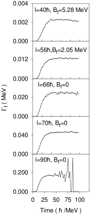
FIG. 1.: Time development of fission widths calculated for the compound nucleus ²⁰⁰Pb at a temperature of 2 MeV for different nuclear spins $l$. The corresponding values of the fission barriers $B_{f}$ are also given.

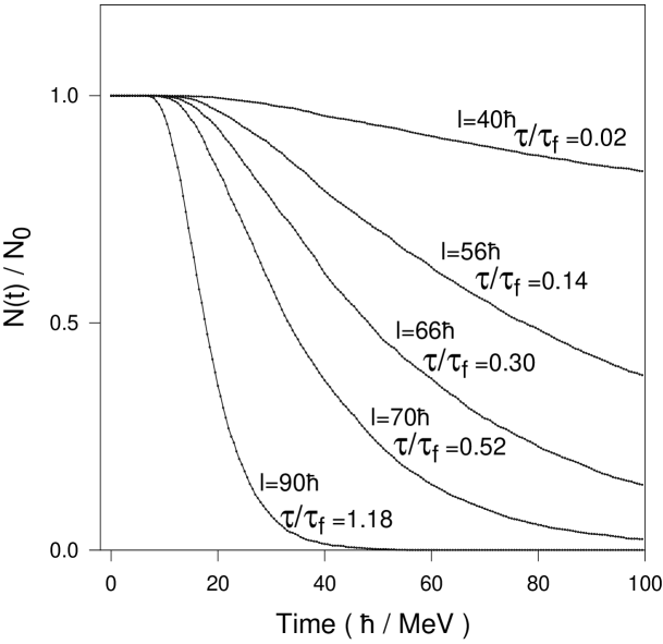
FIG. 2.: Survival probability of the compound nucleus ²⁰⁰Pb against fission at a temperature of 2 MeV for different nuclear spins $l$. The corresponding values of the ratio of the transient time to the fission life time ($\tau/\tau_{f}$) are also given.

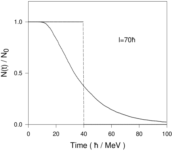
FIG. 3.: Survival probability of the compound nucleus ²⁰⁰Pb against fission at a temperature of 2 MeV calculated with (solid line) and without (dashed line) the random force in the Langevin equation.

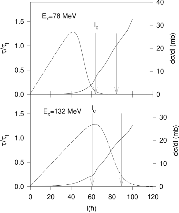
FIG. 4.: The ratio of the transient time to the fission life time ($\tau/\tau_{f}$) as a function of the spin $l$ of the compound nucleus ²⁰⁰Pb at two excitation energies (solid lines). The transition region is indicated by the two arrows. The arrow at the critical angular momentum ($l_{c}$) marks the beginning of the transition region. The next arrow corresponds to $\tau/\tau_{f}=1$ and indicates the end of the transition region. The partial cross sections for compound nucleus formation are also shown (dashed lines).

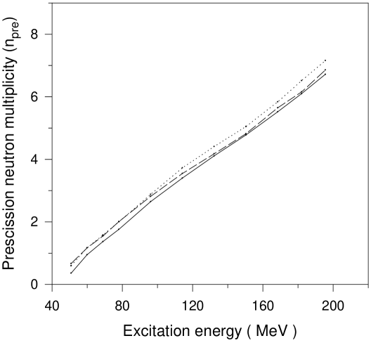
FIG. 5.: Prescission neutron multiplicities calculated from the statistical model with (dotted line) and without (dashed line) the single swoop approximation (see text). Results from the dynamical model (solid line) are also shown.

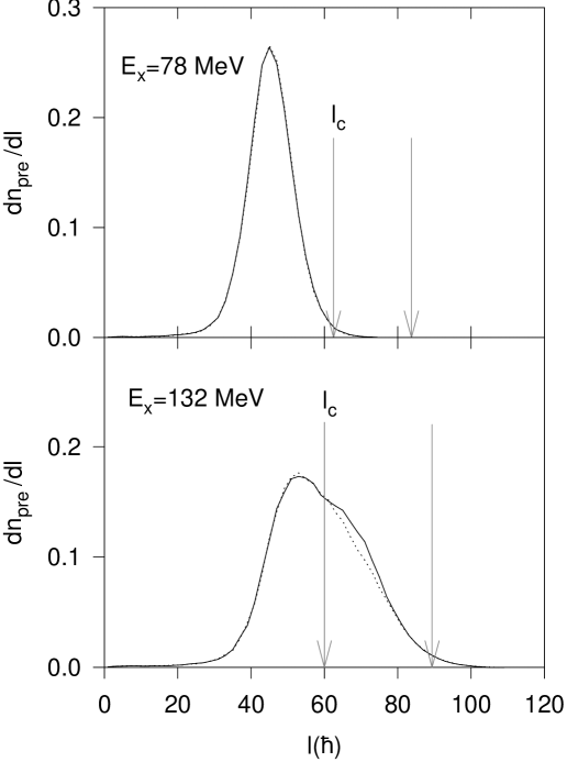
FIG. 6.: Differential prescission neutron multiplicities calculated with the single swoop approximation at two excitation energies (solid lines). The corresponding distributions without the single swoop approximation are shown by the dotted lines. The transition regions are also indicated as in fig.4.

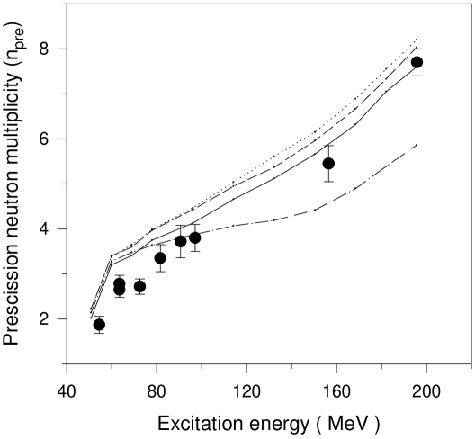
FIG. 7.: Prescission neutron multiplicities calculated from the statistical model with (dotted line) and without (dashed line) the single swoop approximation and also from the dynamical model (solid line) along with the experimental data. The results of a statistical calculation using the stationary values of the fission widths are also shown (dash-dotted line).

REFERENCES

- [1] M. Thoennessen and G.F. Bertsch, Phys. Rev. Lett. 71, 4303 (1993).
- [2] H.A. Kramers, Physica (Amsterdam) 4, 284 (1940).
- [3] P. Grange, S. Hassani, H. A. Weidenmüller, A. Gavron, J. R. Nix, and A. J. Sierk, Phys. Rev. C34, 209(1986).
- [4] Y. Abe, S. Ayik, P.-G. Reinhard, and E. Suraud, Phys. Rep. 275, 49 (1996).
- [5] P. Fröbrich and I.I. Gontchar, Phys. Rep. 292, 131 (1998).
- [6] P. Grange, Q. Li-Jang, and H.A. Weidenmüller, Phys. Rev. C 27, 2063 (1983).
- [7] P. Grange, Nucl. Phys. A428, 37c(1984).
- [8] P. Grange, Li Jun-Qing and H. A. Weidenmüller, Phys. Rev. C27, 2063(1983).
- [9] H. A. Weidenmüller and Zhang Jing-Shang, Phys. Rev. C29, 879(1984).
- [10] R. Butsch, D. J. Hofman, C. P. Montoya, P. Paul and M. Thoennessen, Phys. Rev. C44, 1515(1991)
- [11] S. Pal and T. Mukhopadhyay, Phys. Rev. C54, 1333 (1996).
- [12] Gargi Chaudhuri and S. Pal, Phys. Rev. C (in press).
- [13] Gargi Chaudhuri and S. Pal, Phys. Rev. C63, 064603 (2001).
- [14] M. Brack, J. Damgard, A.S. Jensen, H.C. Pauli, V.M. Strutinsky, and C.Y. Wong, Rev. Mod. Phys. 44, 320 (1972).
- [15] T. Wada, Y. Abe, and N. Carjan, Phys. Rev. Lett. 70, 3538 (1993).
- [16] K.T.R. Davies, A.J. Sierk, and J.R. Nix, Phys. Rev. C13, 2385 (1976).
- [17] P. Fröbrich, I.I. Gontchar, and N.D. Mavlitov, Nucl. Phys. A556, 281 (1993).
- [18] J. Blocki, Y. Boneh, J.R. Nix, J. Randrup, M. Robel, A.J. Sierk, and W.J. Swiatecki, Ann. Phys. (N.Y.) 113, 330 (1978).
- [19] J. Blocki, F. Brut, T. Srokowski, and W.J. Swiatecki, Nucl. Phys. A545, 511c (1992).
- [20] S.E. Koonin and J. Randrup, Nucl. Phys. A289, 475 (1977).
- [21] M. Baldo, G. F. Burgio, A. Rapisarada, P. Schuck, Phys. Rev. C58, 2821(1998).
- [22] J. Blocki, J-J Shi, and W.J. Swiatecki, Nucl. Phys. A554, 387(1993).
- [23] A.J. Sierk and J. R. Nix, Phys. Rev. C21, 982 (1980).
- [24] J.O. Newton, D.J. Hinde, R.J. Charity, R.J. Leigh, J.J.M. Bokhorst, A. Chatterjee, G.S. Foote, and S. Ogaza, Nucl. Phys. A483, 126 (1988).
- [25] D.J. Hinde, D. Hilscher, H. Rossner, B. Gebaure, M. Lehmann, and M. Wilpert, Phys. Rev. C45, 1229 (1992).
- [26] D.J. Hinde, H. Ogata, M. Tanaba, T. Shimoda, N. Takahashi, A. Shinohara, S. Wakamatsu, K. Katori, and H. Okamura, Phys. Rev. C39, 2268 (1989).
- [27] N.D. Mavlitov, P. Fröbrich, and I.I. Gonchar, Z. Phys. A 342, 195 (1992).