One-loop corrections to $\bm{\omega}$ photoproduction near threshold

Abstract

One-loop corrections to $\omega$ photoproduction near threshold have been investigated by using the approximation that all relevant transition amplitudes are calculated from the tree diagrams of effective Lagrangians. With the parameters constrained by the data of $\gamma N\to\pi N$, $\gamma N\to\rho N$, and $\pi N\to\omega N$ reactions, it is found that the one-loop effects due to the intermediate $\pi N$ and $\rho N$ states can significantly change the differential cross sections and spin observables. The results from this exploratory investigation suggest strongly that the coupled-channel effects should be taken into account in extracting reliable resonance parameters from the data of vector meson photoproduction in the resonance region.

I Introduction

Experimental data of vector meson photoproductions are now being rapidly accumulated at Bonn Klein96-98 , Thomas Jefferson National Accelerator Facility CLAS , GRAAL of Grenoble GRAAL01 , and LEPS of SPring-8 LEPS01 . The study of photoproduction of vector mesons ($\omega,\rho,\phi$) is expected to be useful to resolve the so-called “missing resonances” problem CR00 . In addition, the extracted resonance parameters can shed lights on the structure of nucleon resonances ($N^{*}$) and can be used to test the existing hadron models. In recent years, some theoretical progress has been made ZLB98c-Zhao01 ; OTL01 in this direction. In this work we will address the question about how these earlier models should be improved for a more reliable extraction of the $N^{*}$ parameters from the forthcoming data. To be specific, we consider the photoproduction of $\omega$ meson.

It is well known that the extraction of $N^{*}$ parameters from experimental data depends strongly on the accuracy of the treatment of the non-resonant amplitudes. In all of the recent studies of $\omega$ photoproduction at resonance region ZLB98c-Zhao01 ; OTL01 , the non-resonant amplitudes are calculated from the tree diagrams of effective Lagrangians. This is obviously not satisfactory for the following reasons. First, the tree-diagram models do not include the hadronic final state interaction (FSI). The importance of FSI in interpreting the data has been demonstrated in the study of pion photoproductions. For example, the calculations of Ref. SL96 have shown that the magnetic $M1$ amplitude of the $\gamma N\rightarrow\Delta(1232)$ transition can be identified with the predictions from constituent quark models only when the pion re-scattering effects (i.e., pion cloud effects), as required by the unitary condition, are accounted for appropriately in analyzing the data. Second, the vector meson productions occur in the energy region where several meson-nucleon channels are open and their influence must be accounted for. This coupled-channel effect was already noticed and explored in 1970’s for vector meson photoproduction SS68 . In this paper we make a first attempt to re-investigate this problem in conjunction with the approach developed in Ref. OTL01 .

In a dynamical formulation, such as that developed in Ref. SL96 , the most ideal approach is to carry out a coupled-channel calculation. At energies near the $\omega$ photoproduction threshold, the meson-baryon channels which must be included in a coupled-channel calculation are many, such as $\pi N$, $\pi\Delta$, $\rho N$, and $KY$. Such a full coupled-channel calculation is not feasible at the present stage, mainly because some of the experimental information that are needed to constrain the transitions between relevant hadronic meson-baryon channels are not available. For example, there is no information about $\pi\Delta\to\omega N$ and $KY\to\omega N$ transitions. We therefore are only able to consider just the effects due to intermediate $\pi N$ and $\rho N$ channels. In this exploratory investigation, we will follow Ref. SS68 to further simplify the calculations by only considering the one-loop corrections which are the leading order terms in a perturbation expansion of a full coupled-channel formulation, as will be explained in Sec. II. Nevertheless, our results will shed some lights on the importance of coupled-channel effects and provide information for developing a much more complex full coupled-channel calculation. In many respects, our investigation is similar to a recent investigation of coupled-channel effects on kaon photoproduction CTLS01 .

This paper is organized as follows. In Sec. II, we introduce a coupled-channel formulation of $\gamma N$ reaction and indicate the procedures for calculating the one-loop corrections to $\omega$ photoproduction. Section III is devoted to specify various transition amplitudes which will be used as the inputs to our calculations. Numerical results are presented and discussed in Sec. IV. The conclusions are given in Sec. V. Some details on the $\pi N\to\omega N$ reaction are given in Appendix.

II Dynamical Coupled-Channel Formulation

In the considered energy region, the $\gamma N$ reaction is a multi-channel multi-resonance problem. In this work we follow the dynamical approach developed by Sato and Lee SL96 to investigate this problem. It is done by simply extending the scattering formulation of Ref. SL96 to include more $N^{*}$ states and more meson-nucleon channels. The resulting amplitude $T_{\gamma N,\omega N}(E)$ for the $\gamma N\rightarrow\omega N$ reaction can be written as

$$T_{\gamma N,\omega N}(E)=t_{\gamma N,\omega N}(E)+\sum_{N^{*}}\frac{\bar{\Gamma}_{\gamma N\rightarrow N^{*}}\bar{\Gamma}_{N^{*}\rightarrow\omega N}}{E-M_{N^{*}}^{0}-\Sigma_{N^{*}}(E)},$$ (1)

where $t_{\gamma N,\omega N}$ is the non-resonant amplitude. It is defined by the following coupled-channel equations

$$t_{\gamma N,\omega N} = B_{\gamma N,\omega N}+\sum_{\alpha}B_{\gamma N,\alpha}G_{\alpha}(E)t_{\alpha,\omega N},$$ (2)

$$t_{\alpha,\beta} = v_{\alpha,\beta}+\sum_{\delta}v_{\alpha,\delta}G_{\delta}(E)t_{\delta,\beta},$$ (3)

where $\alpha,\beta$ denote the considered meson-nucleon channels such as $\omega N$, $\pi N$, $\rho N$, $\pi\Delta$, and $KY$. $B_{\gamma N,\alpha}$ is the non-resonant photoproduction amplitude, $v_{\alpha,\beta}$ are the non-resonant meson-nucleon interactions, and $G_{\alpha}$ is the free meson-nucleon propagator defined by

$$G_{\alpha}(E)=\frac{1}{E-\left(H_{0}\right)_{\alpha}+i\epsilon}.$$ (4)

Here $(H_{0})_{\alpha}$ is the free Hamiltonian in channel $\alpha$. For channels containing an unstable particle, such as $\rho N$ and $\pi\Delta$, their widths must be included appropriately. Here we follow the procedure of Ref. LEE84 .

The $N^{*}$ excitations are described by the second term of Eq. (1). It is defined by the dressed vertex functions

$$\bar{\Gamma}_{\gamma N\rightarrow N^{*}} = {\Gamma_{\gamma N\rightarrow N^{*}}}+\sum_{\alpha}v_{\gamma N,\alpha}G_{\alpha}(E)\bar{\Gamma}_{\alpha\rightarrow N^{*}},$$

$$\bar{\Gamma}_{N^{*}\rightarrow\omega N} = \Gamma_{N^{*}\rightarrow\omega N}+\sum_{\alpha}\Gamma_{N^{*}\rightarrow\alpha}G_{\alpha}(E)t_{\alpha,\omega N},$$ (5)

and the $N^{*}$ self-energy

$$\Sigma_{N^{*}}(E) = \sum_{\alpha}\bar{\Gamma}_{N^{*}\rightarrow\alpha}G_{\alpha}(E)\Gamma_{\alpha\rightarrow N^{*}}.$$ (6)

The bare mass $M^{0}_{N^{*}}$ of Eq. (1) and the bare vertices $\Gamma_{\gamma N\leftrightarrow N^{*}}$ and $\Gamma_{\alpha\leftrightarrow N^{*}}$ of Eq. (5) can be identified with the predictions from a hadron model that does not include the continuum meson-baryon states.

In this paper, we focus on the calculation of the non-resonant amplitudes defined by Eqs. (2) and (3). The extraction of resonance parameters from the data depends heavily on the accuracy of this dynamical input. At energies near the $\omega$ production threshold, the hadronic meson-baryon channels that must be included in solving Eqs. (2) and (3) are many, such as $\pi N$, $\omega N$, $\rho N$, $\pi\Delta$, and $KY$. Because of the data which are needed to constraint the interaction $v_{\alpha,\beta}$ of Eq. (3) are very limited, we are only able to consider the effects due to the intermediate $\pi N$ and $\rho N$ channels. To further simplify the investigation, we make the one-loop approximation that the amplitude in Eq. (2) is evaluated by setting $t_{\alpha,\beta}\sim v_{\alpha,\beta}$. No attempt is made to solve the coupled-channel equation (3). Furthermore, we assume that the interaction $v_{\alpha,\beta}$ can be calculated from the tree diagrams of effective Lagrangians. This is certainly not very satisfactory, but it should be sufficient for this exploratory study.

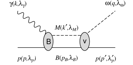
Figure 1: Diagramatic representation of the intermediate meson-baryon (MB) state in $\omega$ photoproduction.

Our task in this work is therefore to investigate the non-resonant amplitude $t_{\gamma N,\omega N}$ defined by Eq. (2), with $t_{\alpha,\omega N}$ replaced by $v_{\alpha,\omega N}$. The second term of Eq. (2) is then the one-loop correction represented graphically in Fig. 1. Explicitly, the matrix element of this one-loop amplitude in the center of mass frame is

$$t^{\mbox{\scriptsize one-loop}}_{\gamma N,\omega N}({\bf k},{\bf q};E)=\sum_{M=\pi,\rho}\int d{\bf q^{\prime}}B_{\gamma N,MN}({\bf k},{\bf q^{\prime}};E)G_{MN}({\bf q^{\prime}},E)v_{MN,\omega N}({\bf q^{\prime}},{\bf q};E),$$ (7)

where ${\bf k}$ and ${\bf q}$ are the momenta for the incoming photon and the intermediate mesons, respectively. The propagator for the $\pi N$ state is

$$G_{\pi N}({\bf q^{\prime}},E)=\frac{1}{E-E_{N}({\bf q^{\prime}})-E_{\pi}({\bf q^{\prime}})+i\epsilon}.$$ (8)

For the $\rho N$ propagator, we account for the width of the $\rho$ by using the the approach of Ref. LEE84 . Neglecting the energy-dependence of the mass shift term, the $\rho N$ propagator takes the following form

$$G_{\rho N}({\bf q^{\prime}},E)=\frac{1}{E-E_{N}({\bf q^{\prime}})-E_{\rho}({\bf q^{\prime}})+i\frac{\Gamma\bm{(}\omega(q^{\prime},E)\bm{)}}{2}\theta[\omega^{2}(q^{\prime},E)-4M^{2}_{\pi}]},$$ (9)

where $\omega(q^{\prime},E)=[(E-E_{N}(q^{\prime}))^{2}-q^{{}^{\prime}2}]^{1/2}$ is the energy available for the $\rho$ meson in its rest frame, and the step function is $\theta(x)=1$ for $x\geq 0$ and $0$ otherwise. The width is

$$\Gamma(\omega)=\Gamma^{0}_{\rho}\frac{k^{3}E_{\pi}(k)}{k^{3}_{0}E_{\pi}(k_{0})}\left(\frac{\Lambda^{2}_{\rho}+k^{2}_{0}}{\Lambda^{2}_{\rho}+k^{2}}\right)^{4},$$ (10)

where $k$ is defined by $\omega=2E_{\pi}(k)$ and $k_{0}$ by $M_{\rho}=2E_{\pi}(k_{0})$. (The above form can be derived from a resonant model for fitting the $\pi\pi$ scattering phase shifts in the $J=I=1$ channel with a $\rho\to\pi\pi$ vertex interaction.) We set $\Gamma^{0}_{\rho}=150$ MeV and $\Lambda_{\rho}=0.5$ GeV.

In the following Section, we describe how the matrix elements of $B_{\gamma N,MN}$ and $v_{MN,\omega N}$ are calculated from effective Lagrangians and constrained by experimental data.

III Non-Resonant Amplitudes

We assume that all non-resonant amplitudes $B_{\gamma N,MN}$ and $v_{MN,\omega N}$ in the one-loop term in Eq. (7) can be calculated from the tree-diagrams defined by the following effective Lagrangian,

$${\cal L}={\cal L}_{V\gamma\varphi}+{\cal L}_{VV\varphi}+{\cal L}_{\varphi NN}+{\cal L}_{\sigma}+{\cal L}_{\gamma NN}+{\cal L}_{VNN},$$ (11)

where

$${\cal L}_{V\gamma\varphi} = \frac{eg_{\rho\gamma\pi}}{2M_{\rho}}\varepsilon^{\mu\nu\alpha\beta}\,\mbox{Tr}\,[\partial_{\mu}\rho_{\nu}\partial_{\alpha}A_{\beta}\pi]+\frac{eg_{\omega\gamma\pi}}{2M_{\omega}}\varepsilon^{\mu\nu\alpha\beta}\,\mbox{Tr}\,[\partial_{\mu}\omega_{\nu}\partial_{\alpha}A_{\beta}\pi\tau^{3}]$$

$$\mbox{}+\frac{eg_{\omega\gamma\eta}}{M_{\omega}}\varepsilon^{\mu\nu\alpha\beta}\partial_{\mu}\omega_{\nu}\partial_{\alpha}A_{\beta}\eta,$$

$${\cal L}_{VV\varphi} = \frac{g_{\omega\rho\pi}}{2}\varepsilon^{\mu\nu\alpha\beta}\,\mbox{Tr}\,[\partial_{\mu}\omega_{\nu}\partial_{\alpha}\rho_{\beta}\pi],$$

$${\cal L}_{\varphi NN} = \frac{g_{\pi NN}}{2M_{N}}\bar{\psi}\gamma^{\mu}\gamma_{5}\partial_{\mu}\pi\psi+\frac{g_{\eta NN}}{2M_{N}}\bar{\psi}\gamma^{\mu}\gamma_{5}\psi\partial_{\mu}\eta,$$

$${\cal L}_{\sigma} = g_{\sigma NN}\bar{\psi}\sigma\psi+\frac{eg_{\rho\gamma\sigma}}{2M_{\rho}}\,\mbox{Tr}\,[\tau^{3}\partial_{\mu}\rho_{\nu}\left(\partial^{\mu}A^{\nu}-\partial^{\nu}A^{\mu}\right)\sigma],$$

$${\cal L}_{\gamma NN} = e\bar{\psi}\left(\gamma_{\mu}\frac{1+\tau_{3}}{2}A^{\mu}-\frac{\kappa_{N}}{2M_{N}}\sigma^{\mu\nu}\partial_{\nu}A_{\mu}\right)\psi,$$

$${\cal L}_{VNN} = \frac{g_{\rho NN}}{2}\bar{\psi}\left(\gamma_{\mu}\rho^{\mu}-\frac{\kappa_{\rho}}{2M_{N}}\sigma^{\mu\nu}\partial_{\nu}\rho_{\mu}\right)\psi+g_{\omega NN}\bar{\psi}\left(\gamma_{\mu}\omega^{\mu}-\frac{\kappa_{\omega}}{2M_{N}}\sigma^{\mu\nu}\partial_{\nu}\omega_{\mu}\right)\psi,$$ (12)

where $\pi$ ($=\bm{\tau}\cdot\bm{\pi}$), $\eta$, $\rho_{\mu}$ ($=\bm{\tau}\cdot\bm{\rho}_{\mu}$), and $\omega_{\mu}$ are the pion, eta, rho, and omega meson fields, respectively. The photon field is represented by $A_{\mu}$, and $\psi$ and $\sigma$ are the nucleon and $\sigma$ meson fields, respectively. $M_{N}$ ($M_{V}$) is the nucleon (vector meson) mass and $\kappa_{N}$ is the anomalous magnetic moment of the nucleon, $\kappa_{p}=1.79$ and $\kappa_{n}=-1.91$. Throughout this work we use the convention that $\varepsilon^{0123}=+1$.

The coupling constants of the Lagrangian (12) are determined as follows. First the coupling constants in ${\cal L}_{V\gamma\varphi}$ are determined by the vector meson radiative decay widths given by the Particle Data Group (PDG) PDG00 . In $\mathcal{L}_{VV\varphi}$, the coupling $g_{\omega\rho\pi}$ has been estimated by many models including the massive Yang-Mills approach KRS84-JJMP88 , the hidden gauge approach FKTU85 , the vector meson dominance model KKW96 , the unitary effective resonance model KVR01 , and QCD sum rules EIK83 . All of these models predict that the value of $g_{\omega\rho\pi}$ is in the range of $10$–$16$ GeV^-1. In this work we use $g_{\omega\rho\pi}=12.9$ GeV^-1 TKR01 .

For $\mathcal{L}_{\varphi NN}$, we use the well-known value $g_{\pi NN}^{2}/4\pi=14.0$ and $g_{\eta NN}^{2}/4\pi=0.99$ determined OTL01 ; TLTS99 by using the SU(3) relation. For $\sigma$ meson, its mass and couplings to the nucleon and the vector mesons are highly model-dependent. Following Ref. FS96 , we set $M_{\sigma}=0.5$ GeV and determine the coupling constants of the $\sigma$ meson by reproducing the experimental data of $\rho$ photoproduction at low energies, as explained in Refs. FS96 ; OTL00 . Since the branching ratio of $\omega\to\pi\pi\gamma$ is very small PDG00 , we do not consider the $\omega\gamma\sigma$ coupling in this model.

Following Refs. OTL01 ; OTL00 , the values of the coupling constants $g_{\omega NN}$ and $g_{\rho NN}$ are taken from the analyses of $\pi N$ scattering, pion photoproduction, and nucleon-nucleon scattering SL96 ; RSY99 . All of the coupling constants used in our calculations are summarized in Table 1.

Table 1: Coupling constants of the effective Lagrangian (11).

coupling	value	coupling	value	coupling	value
$g_{\rho\gamma\pi}$	0.70	$g_{\pi NN}$	13.26	$g_{\rho NN}$	6.12
$g_{\omega\gamma\pi}$	1.82	$g_{\eta NN}$	3.53	$\kappa_{\rho}$	3.1
$g_{\omega\gamma\eta}$	0.42	$g_{\sigma NN}$	10.03	$g_{\omega NN}$	10.35
$g_{\omega\rho\pi}$	12.9	$g_{\rho\gamma\sigma}$	3.0	$\kappa_{\omega}$	0.0

In addition to the tree-diagrams which can be calculated by using the Lagrangian (12), we also include the Pomeron exchange in the amplitudes of vector meson photoproduction DL84-92 ; LM95 ; PL97 , although its contribution is relatively small at low energies. The details of the Pomeron exchange can be found, for example, in Refs. TOYM98 ; OTL01 , and will not be repeated here.

Figure 2: Tree-diagrams for $\gamma p\to\omega p$ which include Pomeron exchange, $\pi$ and $\eta$ exchange, and the direct and crossed nucleon terms.

Figure 3: Tree-diagrams for $\pi N\to\omega N$ which include $\rho$ and $b_{1}$ exchanges and the nucleon pole terms.

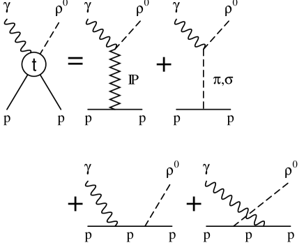
Figure 4: Tree-diagrams for $\gamma p\to\rho p$ which include Pomeron, $\pi$, and $\sigma$ meson exchanges and the nucleon pole terms.

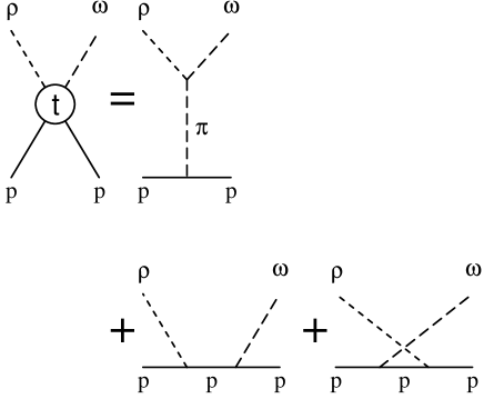
Figure 5: Tree-diagrams for $\rho p\to\omega p$ which include one-pion exchange and the nucleon pole terms.

The considered tree-diagrams are then illustrated in Fig. 2 for $\gamma p\rightarrow\omega p$, Fig. 3 for $\pi N\rightarrow\omega p$, Fig. 4 for $\gamma p\rightarrow\rho^{0}p$, and Fig. 5 for $\rho^{0}p\rightarrow\omega p$. The calculations of these tree-diagrams are straightforward and therefore are not detailed here. These amplitudes are regularized by form factors as follows. For the $t$-channel exchanges, we use

$$F_{t}(t)=\frac{\Lambda^{2}-M_{\rm ex}^{2}}{\Lambda^{2}-t}$$ (13)

for each vertex, where $M_{\rm ex}$ is the mass of the exchanged particle. For the $s$ and $u$ channel diagrams, we include PJ91

$$F_{su}(r)=\frac{\Lambda_{B}^{4}}{\Lambda_{B}^{4}+(r-M_{B}^{2})^{2}},$$ (14)

where $r=(s,u)$ and $M_{B}$ is the mass of the intermediate baryon, i.e., the nucleon in our case. For the cutoff parameters in the tree-diagrams for $\gamma p\to\omega p$, we use the values adopted in Ref. OTL01 ,

$$\Lambda_{\pi NN}=0.6,\qquad\Lambda_{\eta NN}=1.0,\qquad\Lambda_{\omega\pi\gamma}=0.77,\qquad\Lambda_{\omega\eta\gamma}=0.9,\qquad\Lambda_{N}=0.5$$ (15)

in GeV unit and the other cutoff parameters used for the other reactions will be specified later in Sec. IV. The gauge invariance of the nucleon pole terms are restored by making use of the projection operators as in Ref. OTL01 .

The $\gamma N\to\pi N$ amplitudes are not discussed here because no tree-diagram model until now can describe the data in the considered energy region. Instead we construct the non-resonant amplitudes for $\gamma p\to\pi^{0}p$ and $\gamma p\to\pi^{+}n$ by subtracting the resonance amplitudes from the empirical multipole amplitudes of the SAID program said . The $\gamma N\rightarrow\pi N$ resonant amplitudes are calculated by using the procedure given in Ref. DGL02 except that we use the resonance parameters from PDG, not from those of Capstick and Roberts Caps92-CR94 . Clearly, this is very model-dependent approach, but should be sufficient for this very exploratory investigation. The procedures introduced above only define the on-shell matrix elements of $\gamma N\rightarrow\pi N$ transition. For the loop integration (7) we need to define its off-shell behavior. Guided by the work of Ref. SL96 , we assume that

$$B_{\gamma N,\pi N}({\bf k},{\bf q})=B_{\gamma N,\pi N}({\bf k},{\bf q_{0}})\left(\frac{\Lambda^{2}+q^{2}_{0}}{\Lambda^{2}+q^{2}}\right)^{2},$$ (16)

where $\Lambda=0.5$ GeV is chosen. To be consistent, the off-shell extrapolation Eq. (16) is also used in the loop integration over $\rho N$ state.

IV Results and Discussions

We can now perform the calculations based on Eqs. (1) and (7). To proceed, the resonant term of Eq. (1) can be fixed by using the quark model predictions Caps92-CR94 and the procedures detailed in Ref. OTL01 .

In this work, we first consider the one-loop corrections due to the intermediate $\pi N$ channel in Eq. (7). As discussed in the previous Section, the non-resonant $B_{\gamma N,\pi N}$ is generated by using the procedure of Ref. DGL02 to subtract the resonant amplitudes from the empirical $\gamma N\rightarrow\pi N$ amplitudes. Thus our results depend on the employed $\pi N\rightarrow\omega N$ amplitude. To proceed, we adjust the form factors of the tree-diagrams of Fig. 3 to fit the $\pi N\rightarrow\omega N$ data. In addition to the $\rho$ and nucleon exchanges allowed by the Lagrangian (12), we also consider the exchange of the axial vector $b_{1}(1235)$ meson that was considered to explain the $\pi N\rightarrow\omega N$ reaction at high energies. However, we find that its contribution is negligibly small in the considered energy region. The details on the $b_{1}$-exchange amplitude are summarized in Appendix. Our numerical results show that the $\pi^{-}p\rightarrow\omega n$ data near threshold can be described to some extent by choosing the following parameters

$$\Lambda_{\omega\rho\pi}=\Lambda_{\rho NN}=1.55\mbox{ GeV},\qquad\Lambda_{b_{1}\omega\pi}=\Lambda_{b_{1}NN}=1.4\mbox{ GeV},\qquad\Lambda_{N}=0.5\mbox{ GeV}.$$ (17)

The results are the solid lines in Figs. 6 and 7. In the same figure, we also show the results (dashed curves) calculated with

$$\Lambda_{\omega\rho\pi}=\Lambda_{\rho NN}=1.3\mbox{ GeV}.$$ (18)

The dashed curve in Fig. 7 is close to the results from the coupled-channel $K$-matrix model of Ref. PM01a when the resonance contributions and the coupled-channel effects are neglected. We thus interpret that the model corresponding to the dashed curves of Fig. 7 can be used to generate the non-resonant $\pi N\rightarrow\omega N$ amplitude for the calculation according to Eq. (2) or Eq. (7).

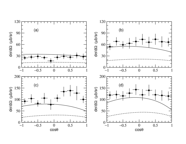
Figure 6: Differential cross section for $\pi^{-}p\to\omega n$ at $W=$ (a) $1.726$ GeV, (b) $1.734$ GeV, (c) $1.746$ GeV, and (d) $1.762$ GeV. The solid lines are obtained with $\Lambda_{\omega\rho\pi}=\Lambda_{\rho NN}=1.55$ GeV and the dashed lines with $\Lambda_{\omega\rho\pi}=\Lambda_{\rho NN}=1.3$ GeV. The experimental data are from Ref. KCDG79 .

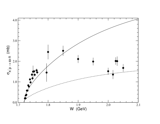
Figure 7: Total cross section for $\pi^{-}p\to\omega n$. Notations are the same as in Fig. 6. The experimental data are from Refs. KCDG79 ; KBCD76-DADD70 .

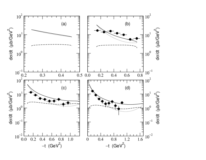
Figure 8: Differential cross section for $\gamma p\to\omega p$ at $E_{\gamma}=$ (a) $1.125$ GeV, (b) $1.23$ GeV, (c) $1.45$ GeV, and (d) $1.68$ GeV, which corresponds to $W=$ (a) $1.73$ GeV, (b) $1.79$ GeV, (c) $1.90$ GeV, and (d) $2.01$ GeV, respectively. The dotted lines are obtained from the tree diagrams and the dashed lines are from the intermediate $\pi N$ channel. The solid lines are the sums of the tree diagrams and the intermediate $\pi N$ channel. The experimental data are from SAPHIR Klein96-98 .

With the non-resonant amplitudes of $\gamma N\rightarrow\pi N$ and $\pi N\rightarrow\omega N$ transition obtained above, we now use Eq. (7) to compute the one-loop corrections due to the intermediate $\pi N$ channel. As shown in Fig. 8, its magnitudes (dashed lines) are smaller than those of the tree-diagrams (dotted lines). However it can have significant effects through its interference with the tree-diagram amplitude. This is evident by comparing the results (solid curves) from the full calculation and the dotted curves. The one-loop corrections are even more dramatic in determining the polarization observables. An example is shown in Fig. 9. We see that the one-loop corrections can change the photon asymmetry in magnitudes at all angles.

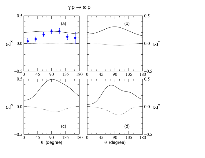
Figure 9: Single photon asymmetry $\Sigma_{x}$ for $\gamma p\to\omega p$ at $E_{\gamma}=$ (a) $1.125$ GeV, (b) $1.23$ GeV, (c) $1.45$ GeV, and (d) $1.68$ GeV. The dotted lines are from the tree diagrams only while the solid lines include the intermediate $\pi N$ channel. The experimental data are from Ref. GRAAL01

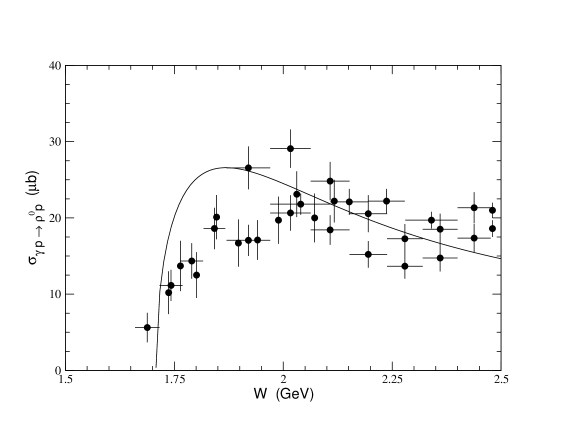
Figure 10: Total cross section for $\gamma p\to\rho^{0}p$. The solid line is obtained with the diagrams of Fig. 4. The experimental data are from Refs. SDEJ72 ; AHHM76 ; ABBH68 ; BCGL69-BCGG72-BCEK73 ; Klein96-98 .

We now turn to investigating the one-loop corrections due to the $\rho N$ channel. From the very limited data AHHM76 ; BDLM79 , we know that $\rho^{\pm}$ photoproduction is much weaker than $\rho^{0}$ photoproduction. We therefore only keep $\rho^{0}p$ in the loop integration (7). The $\rho\Delta$ channel also is not considered by the same reason. The $\gamma p\rightarrow\rho^{0}p$ amplitude is generated from the tree diagrams in Fig. 4 and the $\rho^{0}p\rightarrow\omega p$ amplitude from the tree diagrams in Fig. 5. We note that the tree-diagrams in Fig. 2 and Fig. 5 are related in the vector dominance model, except that the Pomeron and the $\eta$ exchanges are not allowed in $\rho^{0}p\rightarrow\omega p$ transition because of their quantum numbers.

We find that the constructed $\gamma p\rightarrow\rho^{0}p$ amplitude (Fig. 4) can reproduce the total cross section data, if we use the following cutoff parameters (in unit of GeV) OTL00

$$\Lambda_{\pi NN}=0.6,\qquad\Lambda_{\rho\pi\gamma}=0.77,\qquad\Lambda_{\sigma NN}=1.0,\qquad\Lambda_{\sigma\rho\gamma}=0.9,\qquad\Lambda_{N}=0.5.$$ (19)

Our results are shown in Fig. 10. On the other hand, there is no data to constrain our model for $\rho^{0}p\to\omega p$ (Fig. 5). Motivated by vector dominance model, we therefore calculate these tree diagrams using the same form factors, given in Eq. (15), of Fig. 2 for $\omega$ photoproduction. The predicted total cross sections of $\rho^{0}p\rightarrow\omega p$ reaction are shown in Fig. 11. We find that its magnitude at the peak is a factor of about $3$ larger than that in Fig. 7 for the $\pi^{-}p\to\omega n$ reaction. This assumption may lead to an unrealistic estimation of the one-loop corrections due to $\rho N$ channel. Another uncertainty in the calculation of Eq. (7) with $\rho N$ intermediate state is that the correct input to the loop integration (7) is the non-resonant amplitude, not the full amplitudes constructed above. But there is no experimental information we can use here to extract the non-resonant part from the full amplitude. For these reasons, we perform the $\rho N$ loop integration (7) using the constructed full amplitudes of both the $\gamma p\rightarrow\rho^{0}p$ and $\rho^{0}p\rightarrow\omega p$ transitions. Therefore, our results for the $\rho N$ loop can only be considered as an upper bound.

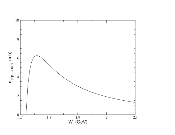
Figure 11: Total cross section for $\rho^{0}p\to\omega p$. The solid line is the result of the diagrams shown in Fig. 5.

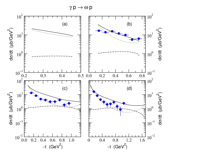
Figure 12: Differential cross section for $\gamma p\to\omega p$ at $E_{\gamma}=$ (a) $1.125$ GeV, (b) $1.23$ GeV, (c) $1.45$ GeV, and (d) $1.68$ GeV. The dotted lines are from the tree diagrams and the dashed lines from the intermediate $\rho N$ channel. The solid lines are the results including the tree diagrams and the intermediate $\pi N$ and $\rho N$ channels. The experimental data are from SAPHIR Klein96-98 .

The calculated one-loop corrections due to the $\rho N$ channel are shown in Fig. 12. Comparison with the results given in Fig. 8 shows that the effects of the $\rho N$ channel are as large as or even bigger than those of the intermediate $\pi N$ channel. Thus the full calculation (solid lines) including both $\pi N$ and $\rho N$ channels gives large corrections to the tree-diagram results (dotted lines). The corresponding coupled-channel effects on photon asymmetry are shown in Fig. 13. Again, we see that the polarization effects are sensitive to the one-loop corrections.

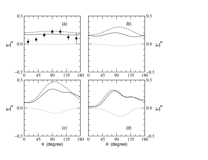
Figure 13: Single photon asymmetry $\Sigma_{x}$ for $\gamma p\to\omega p$ at $E_{\gamma}=$ (a) $1.125$ GeV, (b) $1.23$ GeV, (c) $1.45$ GeV, and (d) $1.68$ GeV. The dotted lines are from the tree diagrams only and the dashed lines include the intermediate $\pi N$ channel. The full calculations including the tree diagrams and the intermediate $\pi N$ and the $\rho N$ channels are given by the solid lines. The experimental data are from Ref. GRAAL01

V Conclusions

As a step toward developing a coupled-channel model of vector meson photoproductions, the one-loop corrections to $\omega$ photoproduction have been investigated. The calculations have been performed by assuming that all relevant non-resonant amplitudes can be calculated from tree-diagrams of effective Lagrangians. Our calculation of the one-loop corrections due to the intermediate $\pi N$ channel is rather well constrained by the data of $\gamma N\rightarrow\pi N$ and $\pi N\rightarrow\omega N$ reactions. On the other hand, our treatment of $\rho N$ channel involves some uncertainties, mainly due to the lack of enough experimental inputs such as the data of $\rho N\rightarrow\omega N$ reaction. Therefore, our results for $\rho N$ channel can only be regarded as an upper bound.

As discussed in section II, the one-loop corrections are just the leading terms of a perturbative expansion of a full coupled-channel model. Thus the results presented in this paper can only be taken as a qualitative indication of the importance of channel coupling effects. We have shown that the one-loop corrections due to intermediate $\pi N$ and $\rho N$ channels are comparable to those of nucleon resonance contributions investigated in Ref. OTL01 . The results from this rather exploratory investigation suggest strongly that the coupled-channel effects should be carefully taken into account in extracting the resonance parameters from the experimental data, in particular the data of polarization observables.

Appendix A The axial $\bm{b_{1}(1235)}$ meson exchange in $\bm{\pi N\to\omega N}$

In this Appendix, we discuss the axial vector $b_{1}(1235)$ meson exchange in $\pi N\to\omega N$ reaction. Recently, this reaction has been studied by effective Lagrangian method and unitary coupled channel models focusing on the role of the nucleon resonances LWF99 ; LWF01 ; TKR01 ; PM01 ; PM01a . In the early investigations in 1960’s and 1970’s this reaction was studied in some detail mostly based on Regge theory and absorption models and at higher energies JDGK65 ; Barm66-68 ; HKK68 ; HK71 ; IM74 . Based on the Regge theory, the $b_{1}$ trajectory exchange has been discussed as the secondary exchange process in $\pi N\to\omega N$ in addition to the major $\rho$-trajectory exchange. The main motivation for the secondary exchange was to account for the experimentally observed non-vanishing vector meson density matrix $\rho_{00}$ that is expected to vanish if the natural-parity $\rho$-trajectory exchange dominates. The $b_{1}(1235)$ meson has quantum numbers $I^{G}(J^{PC})=1^{+}(1^{+-})$ with mass $M_{b_{1}}=1230$ MeV and width $\Gamma_{b_{1}}=142\pm 9$ MeV, and it mostly decays into the $\omega\pi$ channel PDG00 . Thus its exchange can contribute to $\pi N\to\omega N$ as an unnatural parity exchange. In this work we consider the one-$b_{1}$-exchange process (not the exchange of $b_{1}$ trajectory) in $\pi N\to\omega N$.

The general form of the $b_{1}\omega\pi$ interaction can be written as BD63

$$\mathcal{M}_{b_{1}\omega\pi}=-iM_{b_{1}}\varepsilon^{*}_{\mu}(\omega)\left[fg^{\mu\nu}+\frac{h}{M_{\omega}M_{b_{1}}}q^{\nu}k^{\mu}\right]\varepsilon_{\nu}(b_{1}),$$ (20)

where $k$ and $q$ are the momenta of the $b_{1}$ and $\omega$, respectively, and $\varepsilon_{\mu}(b_{1})$ and $\varepsilon_{\mu}(\omega)$ are their polarization vectors. Then the total decay width reads

$$\Gamma_{b_{1}\to\omega\pi}=\frac{|{\bf q}|}{24\pi}\left\{2f^{2}+\frac{1}{M_{\omega}^{4}}\left(E_{\omega}M_{\omega}f+|{\bf q}|^{2}h\right)^{2}\right\},$$ (21)

where $E_{\omega}$ is the $\omega$ meson energy in the $b_{1}$ rest frame. The unknown coupling constants $f$ and $h$ can then be determined by the decay width and the $D/S$ amplitude ratio in the decay of $b_{1}\to\omega\pi$, where Eq. (20) gives IMR89

$$f^{D}/f^{S}=-\frac{\sqrt{2}\left\{M_{\omega}(E_{\omega}-M_{\omega})f+|{\bf q}|^{2}h\right\}}{M_{\omega}(E_{\omega}+2M_{\omega})f+|{\bf q}|^{2}h},$$ (22)

which is defined from

$$\langle\omega({\bf q},m_{\omega})\pi(-{\bf q})|H_{\rm int}|b_{1}({\bf 0},m_{b})\rangle=if^{S}\delta_{m_{\omega}m_{b}}Y_{00}(\Omega_{q})+if^{D}\sum_{m_{\ell}}\langle 2\,m_{\ell}\,1\,m_{\omega}|1\,m_{b}\rangle Y_{2m_{\ell}}(\Omega_{q}),$$ (23)

where $Y_{\ell m}(\Omega)$ and $\langle j_{1}\,m_{1}\,j_{2}\,m_{2}\mid j\,m\rangle$ are the spherical harmonics and Clebsch-Gordan coefficients, and $m_{\omega}$ ($m_{b}$) is the spin projection along the $z$ axis for the $\omega$ ($b_{1}$) meson. Using the PDG PDG00 values for $\Gamma_{b_{1}\to\omega\pi}$ and $f^{D}/f^{S}$, i.e., $\Gamma_{b_{1}\to\omega\pi}=142\pm 9$ MeV and $f^{D}/f^{S}=0.29\pm 0.04$, we obtain

$$f\approx 3.71,\qquad h\approx-11.38,$$ (24)

which gives $h/f\approx-3.1$. This should be compared with the value $h/f=+9.0$ used by Ref. Barm66-68 to fit the high energy data of $\pi N\to\omega N$ together with the $\rho$-trajectory exchange.

The $b_{1}$-nucleon coupling can be written as

$$\mathcal{M}_{b_{1}NN}=\frac{ig_{b_{1}NN}}{2M_{N}}\bar{\psi}\sigma^{\mu\nu}\gamma_{5}q^{\nu}\bm{\tau}\cdot\bm{b}_{\mu}\psi,$$ (25)

due to the $G$ parity of the $b_{1}$, where $b_{\mu}$ is the $b_{1}$ meson field and $\psi$ is the nucleon. The momentum of the $b_{1}$ meson is denoted by $q_{\mu}$. The coupling constant $g_{b_{1}NN}$ is related to the nucleon tensor charge and has been recently estimated by making use of the axial vector dominance and SU(6) $\times$ O(3) spin-flavor symmetry in Ref. GGo01 in a similar way to Ref. BF96 . (See also Ref. KMOV00 .) The result reads

$$g_{b_{1}NN}=\frac{5}{3\sqrt{2}}g_{a_{1}NN}.$$ (26)

Using $g_{a_{1}NN}\approx 7.49$, one finally obtains $g_{b_{1}NN}\approx 8.83$ GGo01 .

Thus the production amplitude for the reaction of $\pi N\to\omega N$ is obtained as

$$\mathcal{M} = \frac{M_{b_{1}}g_{b_{1}NN}C_{I}}{2M_{N}[(k-q)^{2}-M_{b_{1}}^{2}]}\varepsilon^{*}_{\mu}(\omega)\left\{fg^{\mu\nu}+\frac{h}{M_{\omega}M_{b_{1}}}q^{\nu}(k-q)^{\mu}\right\}$$ (27)

$$\mbox{}\times\left\{g_{\nu\alpha}-\frac{(k-q)_{\nu}(k-q)_{\alpha}}{M_{b_{1}}^{2}}\right\}\bar{u}(p^{\prime})\gamma_{5}\sigma^{\alpha\beta}(k-q)_{\beta}u(p),$$

where $u(p)$ is the Dirac spinor of the nucleon with momentum $p$. The isospin factor $C_{I}$ is

$$C_{I}=\left\{\begin{array}[]{ll}\sqrt{2}&\mbox{ for }\pi^{-}p\to\omega n,\ \pi^{+}n\to\omega p\\ +1&\mbox{ for }\pi^{0}p\to\omega p\\ -1&\mbox{ for }\pi^{0}n\to\omega n\end{array}\right.$$ (28)

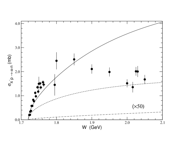
Figure 14: Total cross section for $\pi^{-}p\to\omega n$. Solid and dashed lines are the same as in Fig. 6 while the dot-dashed line is from the $b_{1}(1235)$ exchange process (multiplied by $50$). The experimental data are from Refs. KCDG79 ; KBCD76-DADD70 .

Given in Fig. 14 are the total cross sections for $\pi^{-}p\to\omega n$. The solid and dashed lines are obtained with the $\rho$ exchange and the nucleon pole terms with the cutoff parameters (17) and (18), respectively. The total cross section due to the $b_{1}$ exchange is given by the dot-dashed line. For the form factor, we use the form of Eq. (13) with $\Lambda_{b_{1}\omega\pi}=\Lambda_{b_{1}NN}=1.4$ GeV. Since its contribution is suppressed by $\rho$ and nucleon exchange contributions, the $b_{1}$ exchange is magnified in Fig. 14 by a factor of $50$. This conclusion does not sensitively depend on the cutoff parameters $\Lambda_{b_{1}\omega\pi}$ and $\Lambda_{b_{1}NN}$, when they are larger than the exchanged meson mass $M_{b_{1}}$.

References

- (1) F. J. Klein, Ph.D. thesis, Bonn University (1996); N Newslett. 14, 141 (1998).
- (2) CLAS Collaboration, E. Anciant et al., Phys. Rev. Lett. 85, 4682 (2000); CLAS Collaboration, K. Lukashin et al., Phys. Rev. C 63, 065205 (2001); CLAS Collaboration, M. Battaglieri et al., Phys. Rev. Lett. 87, 172002 (2001).
- (3) J. Ajaka et al., in Proceedings of 14th International Spin Physics Symposium (SPIN 2000), Oct. 2000, Edited by K. Hatanaka, T. Nakano, K. Imai, and H. Ejiri, AIP Conf. Proc. 570, 198 (2001).
- (4) LEPS Collaboration, T. Nakano, in Proceedings of 14th International Spin Physics Symposium (SPIN 2000), Oct. 2000, Edited by K. Hatanaka, T. Nakano, K. Imai, and H. Ejiri, AIP Conf. Proc. 570, 189 (2001).
- (5) S. Capstick and W. Roberts, Prog. Part. Nucl. Phys. 45, S241 (2000), and references therein.
- (6) Q. Zhao, Z. Li, and C. Bennhold, Phys. Rev. C 58, 2393 (1998); Q. Zhao, ibid. 63, 025203 (2001).
- (7) Y. Oh, A. I. Titov, and T.-S. H. Lee, Phys. Rev. C 63, 025201 (2001).
- (8) T. Sato and T.-S. H. Lee, Phys. Rev. C 54, 2660 (1996).
- (9) K. Schilling and F. Storim, Nucl. Phys. B7, 559 (1968).
- (10) W.-T. Chiang, F. Tabakin, T.-S. H. Lee, and B. Saghai, Phys. Lett B 517, 101 (2001).
- (11) T.-S. H. Lee, Phys. Rev. C 29, 195 (1984).
- (12) Particle Data Group, D. E. Groom et al., Eur. Phys. J. C 15, 1 (2000).
- (13) Ö. Kaymakcalan, S. Rajeev, and J. Schechter, Phys. Rev. D 30, 594 (1984); P. Jain, R. Johnson, U.-G. Meissner, N. W. Park, and J. Schechter, ibid. 37, 3252 (1988).
- (14) T. Fujiwara, T. Kugo, H. Terao, S. Uehara, and K. Yamawaki, Prog. Theor. Phys. 73, 926 (1985).
- (15) F. Klingl, N. Kaiser, and W. Weise, Z. Phys. A 356, 193 (1996).
- (16) F. Kleefeld, E. van Beveren, and G. Rupp, Nucl. Phys. A694, 470 (2001).
- (17) V. L. Eletsky, B. L. Ioffe, and Y. I. Kogan, Phys. Lett. 122B, 423 (1983).
- (18) A. I. Titov, B. Kämpfer, and B. L. Reznik, Phys. Rev. C 65, 065202 (2002).
- (19) A. Titov, T.-S. H. Lee, H. Toki, and O. Streltsova, Phys. Rev. C 60, 035205 (1999).
- (20) B. Friman and M. Soyeur, Nucl. Phys. A600, 477 (1996).
- (21) Y. Oh, A. I. Titov, and T.-S. H. Lee, talk at NSTAR2000 Workshop, Jefferson Lab., Feb. 2000 (2000), nucl-th/0004055.
- (22) Th. A. Rijken, V. G. J. Stoks, and Y. Yamamoto, Phys. Rev. C 59, 21 (1999).
- (23) A. Donnachie and P. V. Landshoff, Nucl. Phys. B244, 322 (1984); Phys. Lett. B 296, 227 (1992).
- (24) J.-M. Laget and R. Mendez-Galain, Nucl. Phys. A581, 397 (1995).
- (25) M. A. Pichowsky and T.-S. H. Lee, Phys. Rev. D 56, 1644 (1997).
- (26) A. I. Titov, Y. Oh, S. N. Yang, and T. Morii, Phys. Rev. C 58, 2429 (1998).
- (27) B. C. Pearce and B. K. Jennings, Nucl. Phys. A528, 655 (1991).
- (28) Partial-Wave Analysis Facility (SAID), R. A. Arndt, W. J. Briscoe, R. L. Workman, and I. I. Strakovsky, http://gwdac.phys.gwu.edu.
- (29) D. Dutta, H. Gao, and T.-S. H. Lee, Phys. Rev. C 65, 044619 (2002).
- (30) S. Capstick, Phys. Rev. D 46, 2864 (1992); S. Capstick and W. Roberts, ibid. 49, 4570 (1994).
- (31) H. Karami, J. Carr, N. C. Debenham, D. A. Garbutt, W. G. Jones, D. M. Binnie, J. Keyne, P. Moissidis, H. N. Sarma, and I. Siotis, Nucl. Phys. B154, 503 (1979).
- (32) G. Penner and U. Mosel, Universität Giessen Report (2001), nucl-th/0111024.
- (33) C. Hanhart and A. Kudryavtsev, Eur. Phys. J. A 6, 325 (1999).
- (34) G. Penner and U. Mosel, Phys. Rev. C 65, 055202 (2002).
- (35) J. S. Danburg, M. A. Abolins, O. I. Dahl, D. W. Davies, P. L. Hoch, J. Kirz, D. H. Miller, and R. K. Rader, Phys. Rev. D 2, 2564 (1970); J. Keyne, D. M. Binnie, J. Carr, N. C. Debenham, A. Duane, D. A. Garbutt, W. G. Jones, I. Siotis, and J. G. McEwen, ibid. 14, 28 (1976).
- (36) Aachen-Hamburg-Heidelberg-München Collaboration, W. Struczinski et al., Nucl. Phys. B108, 45 (1976).
- (37) W. Struczinski et al., Nucl. Phys. B47, 436 (1972).
- (38) ABBHHM Collaboration, R. Erbe et al., Phys. Rev. 175, 1669 (1968).
- (39) J. Ballam, G. B. Chadwick, Z. G. T. Guiragossian, A. Levy, M. Menke, P. Seyboth, and G. E. Wolf, Phys. Lett. 30B, 421 (1969); J. Ballam et al., Phys. Rev. D 5, 545 (1972); 7, 3150 (1973).
- (40) D. P. Barber et al., Z. Phys. C 2, 1 (1979).
- (41) M. Lutz, G. Wolf, and B. Friman, Nucl. Phys. A661, 526c (1999).
- (42) M. F. M. Lutz, Gy. Wolf, and B. Friman, Nucl. Phys. A706, 431 (2002).
- (43) M. Post and U. Mosel, Nucl. Phys. A688, 808 (2001).
- (44) J. D. Jackson, J. T. Donohue, K. Gottfried, R. Keyser, and B. E. V. Svensson, Phys. Rev. 139, B428 (1965).
- (45) M. Barmawi, Phys. Rev. 142, 1088 (1966); Phys. Rev. Lett. 16, 595 (1966); Phys. Rev. 166, 1857 (1968).
- (46) F. Henyey, K. Kajantie, and G. L. Kane, Phys. Rev. Lett. 21, 1782 (1968).
- (47) G. E. Hite and E. G. Krubasik, Nucl. Phys. B29, 465 (1971).
- (48) A. C. Irving and C. Michael, Nucl. Phys. B82, 282 (1974).
- (49) S. M. Berman and S. D. Drell, Phys. Rev. Lett. 11, 220 (1963), (E) 11, 303 (1963).
- (50) N. Isgur, C. Morningstar, and C. Reader, Phys. Rev. D 39, 1357 (1989).
- (51) L. Gamberg and G. R. Goldstein, Phys. Rev. Lett. 87, 242001 (2001).
- (52) M. Birkel and H. Fritzsch, Phys. Rev. D 53, 6195 (1996).
- (53) N. I. Kochelev, D.-P. Min, Y. Oh, V. Vento, and A. V. Vinnikov, Phys. Rev. D 61, 094008 (2000).