=3 DANIELLE MOREL dissertation Department of Physics Kirby W. Kemper Chairman Donald J. Foss Doctor of Philosophy 2002 Physics Simon Capstick Ph.D. Gregory Riccardi Jorge Piekarewicz Paul Eugenio Howie Baer Spring Arts and Sciences January 23, 2002 To my family

EFFECTS OF BARYON-MESON INTERMEDIATE STATES ON BARYON MASSES

Acknowledgements       This dissertation could not have been achieved without the support, guidance, and infinite patience of Professor Simon Capstick. I will always be grateful to him for seeing in me the potential to undertake and, despite some rough times, complete this project. I would also like to extend my heartfelt appreciation to Professor Winston Roberts of Old Dominion University, for his help and support through the last year of this project, and to Professor Jorge Piekarewicz of Florida State University, for his keen insights, and unwavering good spirits. Many thanks to Professors Baer, Eugenio, and Riccardi for reviewing this manuscript and offering precious advice. Finally I would like to thank Professors Dennis and Riccardi for giving me access to the computing power of the FSU Department of Physics Computer Cluster without which this project would not have been feasible, and the FSU College of Arts and Sciences for providing the funding necessary to make the cluster a reality.

This work was supported in part by the U.S. Department of Energy under Contract DE-FG02-86ER40273.

ABSTRACT

Chapter 0 Introduction

The field of nuclear physics spans a very wide range of phenomena and, despite a long history, is still riddled with a large number of unanswered questions. Within it, the field of hadron physics finds itself in a ‘bridge’ position between the visible world of atoms where electrons and nuclei rule, and the realm of high energy physics where quarks, gluons, and other such ‘invisible’ elementary forms of matter are the focus of attention. Hadrons are ultimately what our world is made of, i.e. the fundamental pieces of matter bound together to become the neutrons and protons (two examples of hadrons), then further combined to form the nucleus of each atom charted on the periodic table of elements.

Studying hadrons therefore means trying to understand how and why particles like quarks and gluons are combined to produce the experimentally observed spectra of objects labeled ‘mesons’ (predominantly quark + anti-quark + gluons states, such as pions) and ‘baryons’ (predominantly three-quark + gluons states such, as protons and neutrons) as opposed to any other possible combination. Additionally, while an electron can be removed from an atom and isolated to study how forces act upon it, the ‘strong force’ that holds quarks together is so strong that we have not, and according to our current understanding will not, see a single quark in isolation. Matter can be disintegrated down to its quark constituents in highly energetic accelerators but the length of time quarks remain individual particles (i.e. not bound to others) is incredibly short, and ultimately they end up bound to each other in hadrons. Therefore much about the strong force and how it binds quarks into hadrons remains poorly understood.

Not only is the study of the strong interactions pushing the limit of current experimental facilities, but theoretical tools that are known to work well with electromagnetic or high energy phenomena have very limited use in the study of quarks and gluons, at least at the energy scale where they form bound states such as baryons and mesons. In addition, the theory which is now accepted to be correct for strong interaction physics is so complex that the equations governing it can only be solved exactly for a very limited number of cases, leaving sizeable gaps in our understanding.

Theoretical work is therefore ongoing in two main areas. One is to broaden the range of applicability of exact solutions of the theory of strong interactions via novel computing techniques and algorithms. The other is to develop and/or improve models which, although not exact, give a good overall picture of many manifestations of the strong force and open windows to the physics behind many experimentally observed phenomena. Within this context, the broad goal of the work presented in this thesis is to remove a level of approximation in one already successful baryon spectroscopy model, i.e. a model which describes and predicts the number and properties of baryon states that should be ‘seen’ experimentally. Doing so should improve the ability of this model to explain some of the intricacies of the baryon spectrum, while increasing its predictive power and helping resolve some of the discrepancies between predictions and observations.

1 Quantum Chromodynamics

It is now accepted that the building blocks of matter are the quarks, leptons, and gauge bosons. Quarks come in six different species or ‘flavors’, and are known as the up ‘$u$’, down ‘$d$’, strange ‘$s$’, charm ‘$c$’, top ‘$t$’, and bottom ‘$b$’ quarks. The six flavors of leptons are the electron ‘$e^{-}$’, muon ‘$\mu^{-}$’, and tau ‘$\tau^{-}$’ and their associated neutrinos $\nu_{e}$, $\nu_{\mu}$, and $\nu_{\tau}$. Quarks and leptons form a group of particles called fermions. Each has half-integer spin and an associated anti-particle, for example the positron ‘$e^{+}$’ or the anti-top quark ‘$\bar{t}$’, which are identical in mass but different in charge and color (another quark quantum number discussed more below) to their particles. The gauge bosons are integer-spin particles and are the photon ‘$\gamma$’, $Z,W^{\pm}$, gluon ‘$g$’, and the proposed graviton.

There are four fundamental interactions, each with one or more particles associated with it that carry the force. Gravity, the weakest of these interactions, is thought to be mediated by massless, spin-two gravitons. The weak interaction, whose force is carried by spin-one, self-interacting $Z$ and $W^{\pm}$ bosons, is really a component of the electro-weak force and is responsible for radioactive beta decay processes. The other part of this force manifests itself via electromagnetic interactions, which act between electrically charged objects and are mediated by spin-one, electrically neutral photons that do not interact among themselves. Finally, the strong interaction, which acts between color-charged objects, is mediated by self-interacting vector bosons called gluons and is responsible for nuclear binding and the interactions of the constituents of the nuclei. The quarks, which come in three colors and have fractional electric charge, are known to have strong, electromagnetic, weak, and gravitational interactions. The leptons, such as the electron, are subject to all forces except the strong one, as they do not carry a color charge, while the neutrinos have neither strong nor electromagnetic interactions.

The strong force is ‘weak’ at very short distances, creating what is called asymptotic freedom (quarks appear to behave like free particles), but grows infinitely strong at ‘large’ distances, resulting in the phenomenon known as confinement (a quark cannot be isolated like an electron or a proton). The strong interactions provide the ‘glue’ to hold the quarks together to make hadrons, the strongly interacting particles, the mesons and baryons. Although the number of quarks within hadrons is not defined by quantum field theories, several models have baryons composed of three ‘constituent’ quarks, which have half-integer spin and obey Fermi-Dirac statistics. Mesons on the other hand are described as integer spin quark-antiquark pairs that obey Bose-Einstein statistics. To be observable, particles such as hadrons are required by confinement to be colorless objects (color singlets). Baryons must therefore have one red, one blue, and one yellow quark (as $RBY$ = white) and mesons are allowed to be a colorless combination of $R\bar{R}$, $B\bar{B}$, and $Y\bar{Y}$ quark-antiquark pairs. There is growing evidence for the existence of other quark and gluon states such as glueballs (pure gluon states) and hybrids (eg. $qqqg$), as well as hypothesized states such as diquonia ($q{\bar{q}}q{\bar{q}}$), dibaryons ($qqqqqq$), and others.

The equations describing the electromagnetic interactions were formulated by Maxwell and form the basis of Quantum Electrodynamics (QED). Correct theories for weak and strong interactions came later. It is now widely accepted that a field theory equivalent to QED exists for strongly interacting particles and is known as Quantum Chromodynamics (QCD), with gluons mediating the forces between colored quarks, which are analogous to photons. The QCD Lagrangian has the form

$${\cal L}=-\frac{1}{4}F_{\mu\nu a}F_{a}^{\mu\nu}+{\bar{\Psi}}(i{\hbox to0.0pt{D\hss}/}-m)\Psi,$$ (1)

where $D_{\mu}=\partial_{\mu}-igA_{\mu}^{a}t^{a}$ is the covariant derivative, $F_{a}^{\mu\nu}=\partial^{\mu}A_{a}^{\nu}-\partial^{\nu}A_{a}^{\mu}+g\sum f_{abc}A_{b}^{\mu}A_{c}^{\nu}$ is the field tensor, and $A_{a}^{\mu}$ are the gluon fields ($a=1~{}{\rm to}~{}8$). The last term in the field tensor definition indicates that, unlike the photons of QED, gluons interact with each other, giving QCD its non-abelian behavior (for more information on QCD see for example Refs. [1, 2, 3]). Unfortunately, unlike QED, there is as yet no obviously successful way to go from the QCD Lagrangian to a complete understanding of the large number of observed hadrons and their properties. Lattice QCD, a field theory that replaces space-time with a lattice of discretely spaced points (colored sources -quarks- at the junctions and color electric flux lines -mediated by gluons- as links between them), is making visible progress towards that goal by using numerical techniques to solve otherwise unreachable problems, but calculations beyond masses and static properties of the ground states and the lightest negative parity excited baryon states are still in the future. Other methods, such as expansions based on the large $N_{c}$ (number of colors) limit of QCD, and effective field theories (theories that replace part of unknown interactions by physically sound approximations), are limited in their scope and are currently unable to provide the global yet detailed understanding needed for a description of all aspects of strong interaction physics.

2 Non-perturbative QCD and QCD-based Models

It is relatively easy to treat electroweak interactions via perturbation theory (PT), but strong interactions of hadrons involve dealing with QCD, where one cannot expect much of PT in a situation that is fundamentally not one of weak coupling, as is explained below.

The usual way to treat local interactions is through PT, i.e. by expanding various quantities in powers of the coupling constant. In QED, it is useful to define an effective coupling constant $\alpha(Q^{2})$, which gives the momentum transfer ($Q^{2}$) dependence of the renormalized vertex function. This function receives contributions from vacuum polarization graphs which describe the electron loop corrections to the photon propagator. The result is an effective coupling $\alpha(Q^{2})$ which increases with $Q^{2}$. In QCD however, this situation is complicated by the gluon self-interactions (gluons carry color charge). The effective quark-gluon vertex can be summed over all orders of the renormalized coupling (see figure 1) and has the form

$$\alpha_{s}(Q^{2})=\frac{12\pi}{(33-2N_{f})ln(Q^{2}/\Lambda_{QCD}^{2})}.$$ (2)

where $N_{f}$ is the number of flavors, and $\Lambda_{\rm QCD}$ is the momentum scale at which $\alpha_{s}$ becomes strong as $Q^{2}$ is decreased.

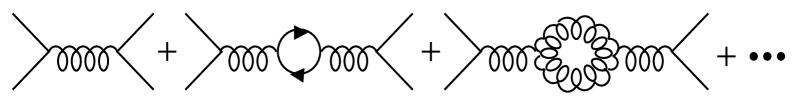
Figure 1: Perturbative expansion of the gluon-gluon interactions defining the strong coupling constant $\alpha_{s}(Q^{2})$.

From Eq. 2 it can be seen that at large $Q^{2}$, or short distances (relative to the $\Lambda_{\rm QCD}$ scale and for $N_{f}\leq 16$), $\alpha_{s}(Q^{2})\rightarrow 0$ (a property known as asymptotic freedom) so that hard processes (processes calculable using perturbative QCD as the momentum transfer is large enough to produce a small value of $\alpha_{s}$) such as deep inelastic scattering, some weak decays of heavy flavors, and some experimentally seen but theoretically highly suppressed strong decays of heavy quarkonia, can successfully be treated perturbatively. On the other hand, at small momentum transfers, or large distances, $\alpha_{s}(Q^{2})$ grows quite large and PT becomes invalid. Unfortunately, this is the region relevant to strong decays of hadrons composed of light quarks, electromagnetic transitions, and the weak decays of hadrons containing light flavors, like hyperons (baryons containing one or more strange quarks) or kaons (mesons containing one strange quark or anti-quark). Experimental measurements yield a value of $\Lambda_{\rm QCD}\approx 200$ MeV. The strong interactions become strong at distances larger than $\sim 1/\Lambda\approx 1$ fm, which is roughly the size of the light hadrons.

Within QCD, there are two main phenomena that are essentially non-perturbative and therefore cannot be obtained even by summing entire perturbative series. The first is confinement, and the second is the dynamical breaking of chiral symmetry. Confinement is related to the interaction energy, which increases with distance in contrast to the Coulomb energy. The breaking of chiral symmetry gives a dynamical mass of several hundred MeV to light quarks, which are known to have current-quark masses of only a few MeV at large momentum scales. Both phenomena are connected to non-zero vacuum expectation values, which would vanish at any order of PT: the so-called quark ($<q\bar{q}>$) and gluon ($<gg>$) condensates.

There are two main alternatives to PT based on field theory. One is the QCD duality sum rules approach, which uses a short distance expansion of products of operators. This method allows certain quantities to be calculated in terms of the condensates $<q\bar{q}>$, $<gg>$, and perturbatively calculable coefficients. These quantities can also be calculated in terms of hadron properties such as masses, widths, and branching ratios, hence the duality. The other is lattice QCD, which attempts to completely calculate hadronic properties from first principles (the QCD Lagrangian on a lattice of space-time points based on the work of Wilson [4], see Ref. [5] for an introduction to lattice QCD) based on the physical idea that the long-distance properties of QCD are the most important (confinement and dynamical breaking of chiral symmetry), and that short distance properties can be reached by extrapolation. These techniques permit strong coupling calculations based on the assumption that the unrenormalized coupling constant is very large, which use Monte Carlo simulations based on Feynman path-integrals.

Recently a covariant approach to the description of hadron structure has been developed, based on the Bethe-Salpeter equation and the Schwinger-Dyson method of solving field theory. This approach has been widely developed for the description of meson, but so far restricted to the descriptions of ground-state baryons.

Although these methods are increasingly useful, they remain technically very complex and somewhat limited in their applicability. Additionally, using these techniques, it is often difficult to obtain physical insight (especially on the lattice) about phenomena such as decay mechanisms or confinement (although confinement is a natural consequence of the lattice, i.e. the area of the Wilson loop gives an energy $\propto r$ so produces a linearly rising potential, it is not a proof of its existence). This highlights the continued need for other methods which are inspired by QCD but not necessarily derived from it. The inability to calculate with QCD in the low $Q^{2}$ regime has made it necessary to use phenomenological models of hadron structure based on expectations of the low energy behavior of QCD. The quark potential model and other dynamical models were created to fulfill this purpose.

Within the framework of the quark potential model, the spectra of mesons and baryons, as well as their strong, weak, and electromagnetic decays have been successfully calculated. This model allows for direct calculation of relevant matrix elements for each definite decay and provides transparent direct links to experimental data. Its simplicity implies a lack of theoretical foundation in QCD, but despite that fact its past and present empirical successes are impressive.

3 Corrections to the Quark Model

In QCD there are $qqq(q\bar{q})$ configurations possible in baryons, and these must have an effect on the constituent quark model, similar to the effect of unquenching lattice QCD calculations. These effects can be modeled by allowing baryons to include baryon-meson (BM) intermediate states, which lead to baryon self energies and mixings of baryons of the same quantum numbers. A calculation of these effects requires a model of baryon-baryon-meson (BB^′M) vertices and their momentum dependence. It is also necessary to have a model of the spectrum and structure of baryon states, including states not seen in analyses of experimental data, in order to provide wave functions for calculating the vertices, and to know the thresholds associated with intermediate states containing missing baryons.

The goal of the present work is to self-consistently calculate such effects for a set of experimentally well known baryon states. The method and results are presented as follows. In Chapter 1 the work of several authors who have made contribution to this field is reviewed, and important elements are extracted and related to the present work. The nature and extent of the present research is then discussed in more detail, highlighting the improvements needed to be made to this type of calculation. Chapters 2 and 3 present an overview of the different methods adopted for use in this research. Results are then presented in detail in Chapter 4, and finally Chapter 5 offers conclusions and outlook for future extensions of this work.

Chapter 1 Baryon Self Energies

Baryon self energies due to BM intermediate states and BM decay widths can be found from the real and imaginary parts of loop diagrams (see Figure 1). The size of such self energies can be expected to be comparable to baryon widths. For this reason, they cannot be ignored when comparing the predictions of any quark model with the results of analyses of experiments. Since the splittings between states which result from differences in self energies can be expected to be comparable to those that arise from the residual interactions between the quarks, a self-consistent calculation of the spectrum needs to adjust the residual interactions, and with them the wave functions of the states used to calculate the BB^′M vertices, to account for these additional splittings.

Earlier studies have brought these facts to the attention of the nuclear physics community, each highlighting different aspects of the problem. What seems to be missing is a consistent and complete calculation of the effects of the self energies on the baryon spectrum. By looking back at the existing literature, lessons can be learned on how to accomplish such a task as thoroughly as possible.

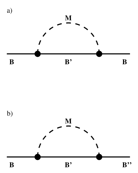
Figure 1: Contributions from a baryon-meson loop to a) the self energy of baryon $B$ and b) the mixing of baryons with same quantum numbers. The dashed arc represents a virtual meson.

1 Existing Work

Previous calculations of the self energies of ground state and negative-parity excited baryons use baryon-meson intermediate states consisting of ground states. The work of Zenczykowksi [6] takes the point of view that the ‘residual’ interquark interactions are unimportant, and that hadronic loop effects dominate the observed splitting and mixing pattern of the ground and first (negative-parity) excited states of baryon states in the octet and decuplet SU(3)_f representations.

This work claims that at least two thirds of the observed splittings in these states can be attributed to such effects, as can the mixing angles between states due to these effects. In a simplifying limit, a formula relating the $\Sigma-\Lambda$ and $\Delta-N$ mass differences, derived using one-gluon exchange by de Rujula, Georgi, and Glashow [7], can be attributed to the effects of hadronic loops.

This calculation uses only spatial ground state intermediate baryons, but unlike those of some other authors, considers a complete set of accessible SU(3)_f intermediate states. This means that for $N$ and $\Delta$ baryons the intermediate states with pseudoscalar mesons were $N\pi$, $\Delta\pi$, $N\eta$, $\Delta\eta$, $N\eta^{\prime}$, $\Delta\eta^{\prime}$, $\Sigma K$, $\Lambda K$, $\Sigma^{*}K$, and those with vector mesons were $N\rho$, $\Delta\rho$, $N\omega$, $\Delta\omega$, $\Sigma K^{*}$, $\Lambda K^{*}$, and $\Sigma^{*}K^{*}$. This calculation also considered the self energies of strange baryons, where a different (and larger) set of intermediate states is possible. A dispersion integral relates the shift in the squared mass of a baryon state to properties of the intermediate states and a spectral function $\rho(s,m_{B}^{\prime},m_{M})$, which depends on the nature of the baryons $B$ (initial) and $B^{\prime}$ (intermediate) involved in the loop diagram,

$$m_{B}^{2}-(m_{B}^{0})^{2}=\sum_{i}w_{i}^{B}\int_{s^{(i)}_{\rm thr}}{\rho(s,m_{B}^{\prime},m_{M})\over m_{B}^{2}-s}ds.$$ (1)

Here the sum runs over all (open and closed) decay channels $i={B^{\prime}M}$ with $\sqrt{s^{(i)}_{\rm thr}}=m_{B^{\prime}}+m_{M}$, and the weights $w_{i}^{B}$ give the spin and flavor [SU(6)] overlaps between the $B$ and $B^{\prime}M$ states. For $B$ and $B^{\prime}$ baryons restricted to ground states, and without SU(3)_f breaking in these ground-state baryon wave functions, these weights have the important property that

$$\sum_{i}w_{i}^{B}=48,$$ (2)

for all baryons $B$, as long as the sum runs over all intermediate states $i$ allowed by the quantum numbers. This means that in this symmetry limit the mass shift due to these effects is the same for all of the ground state baryons, and so no mass splittings are generated by loop effects, as might be expected. This observation is critical, as it makes clear that without the inclusion of at least this set of intermediate states, calculations of these effects do not start from the symmetry limit and so cannot be expected to give physically meaningful results.

Away from this limit the nature of the spectral functions $\rho$ becomes important. Their values were calculated using the ${}^{3}P_{0}$ model with universal radii for the mesons and baryons, taking into account the spin, flavor, and spatial structure of the baryons and mesons involved.

The author concludes that, with reasonable hadron radii, about two thirds of the splittings and mixings in ground and negative-parity excited state baryons must arise from hadronic loop effects, and that this allows the use of a significantly smaller coupling constant $\alpha_{s}$ in the quark residual interactions which may explain the rest of the splittings. It is crucial that a ‘complete’ set of SU(6)-related $B^{\prime}M$ intermediate states is employed.

The work of Blask, Huber, and Metsch [8] is similar to that of Zenczkowski, except that vector mesons are not taken into account in the intermediate states, and the point-like mesons are coupled to baryon states using an elementary-meson emission (EME) model with the meson-quark coupling fixed from the $\pi NN$, $K\Lambda N$ and $\eta NN$ coupling constants derived from analyses of experimental data. The recoil energy of the intermediate baryon is neglected, but intermediate state thresholds are given by using the physical masses of the intermediate hadrons. Baryon masses including these loop effects are found by diagonalising an effective Hamiltonian which includes a term for the internal dynamics of the baryon and meson, and an energy-dependent term

$$\delta H_{b}(E)=\hat{H}_{c}{1\over E+i\epsilon-H}\hat{H}_{c},$$ (3)

where $\hat{H}_{c}$ describes the coupling between baryons and mesons and $H$ is the full Hamiltonian.

Similar conclusions about the importance of such effects are made, although this calculation suffers from a point-like treatment of the mesons (leading to overestimated widths for decaying baryon states) and some problems in the resulting spectrum which likely arise from the restricted set of intermediate states. This calculation also hints at a possible cancellation between the spin-orbit effects due to the one-gluon-exchange residual and splittings which arise from the inclusion of $B^{\prime}M$ intermediate states.

Brack and Bhaduri [9] calculate self energies of the nucleon and $\Delta$ ground states only, using only pions as intermediate mesons, but do not restrict the intermediate $N$ and $\Delta$ baryon states to spatial ground states. They find that the difference in the self energies of the nucleon and $\Delta$ ground states converges to within 5 MeV of the large $N$ result when a set of intermediate baryons up to and including the $N=3$ band (second band of negative-parity orbital excitations) states is employed. They find that, in their model, the difference in the pionic self energies of the odd-parity excited states and the ground state converges too slowly to make definite statements.

Part of this trouble with convergence may be due to their model of the $BB^{\prime}M$ amplitudes, which simply attaches a pion to the quarks with a (nonrelativistic) pseudoscalar coupling, with an additional axial form factor

$$F_{\pi}({\bf k}^{2})=1/(1+{\bf k}^{2}/\Lambda_{\pi}^{2}),$$ (4)

with $\Lambda_{\pi}=1275$ MeV, corresponding to the mass of the $a_{1}$ meson. Since their loop amplitudes involve elementary intermediate pions, they include a factor of $1/\omega_{k}$, where $\omega_{k}=\sqrt{{\bf k}^{2}+m_{\pi}^{2}}$ is the pion energy, from the normalization of the wave function of the intermediate pion. This factor is not present in the pion center of mass wave function in nonrelativistic models which treat it as a composite particle. Although the presence of this factor has the effect of further suppression of high-momentum contributions to the integral over the loop momentum, the net result is that it is still likely that the effective pion-nucleon vertex in this model is too soft. In subsequent models and the present work a more rapid decrease of the vertex amplitudes with $k^{2}$ is shown to produce better results for the mass shifts, and can be attributed to an effective size for the operator which creates a constituent quark-antiquark pair (see Geiger and Isgur [10]).

The intermediate states are described by simple unmixed harmonic oscillator wave functions. The excitation spectrum of the intermediate states is taken to be either harmonic oscillator plus zero-range (contact) spin-spin potential, or the Isgur-Karl potential which is modified by anharmonicities in the spin-independent potential, which gives a more realistic spectrum for the energy of the intermediate states. They show that, at least for the nucleon-$\Delta$ splitting, the details of this spectrum are unimportant. It can be expected that they will become very important, however, if this calculation was extended to the self energies of excited states, as these depend crucially on the positions of the thresholds due to the opening of various channels for excited states to decay to excited states.

The important conclusions of this work are: convergence of the nucleon-$\Delta$ mass difference in the sum over excited intermediate states can be demonstrated; it is misleading to include only baryon ground states as intermediate states, as inclusion of excited states reduces the difference in the nucleon and $\Delta$ self energies substantially; their final results depend sensitively on the chosen (axial) radius of the nucleon, as expected, and changing the gluonic hyperfine splitting changes the difference in the self energies of the nucleon and $\Delta$; and if the gluonic hyperfine splittings are too large ($>250$ MeV) it is impossible to fit the observed $\Delta-N$ splitting. It is also noted that one-pion exchange can, with some adjusted parameters (a reduced strength coupling to the quarks), be made to simulate these effects. Poor convergence was found in the calculation of the self energies of the negative-parity excited states, an issue which will be resolved in the present work.

The work of Horacsek, Iwamura and Nogami [11] would appear to partly contradict that of Brack and Bhaduri, with $\Delta-N=20$ MeV from the inclusion of baryon-pion intermediate states. However, the approximation of each intermediate state quark moving in a single central potential (shell model) is used, so that intermediate excited baryon states are described as individual excited quark substates. This means that the intermediate states are far from a basis of hadrons, and so this calculation ignores what we know about the spectrum of confined hadrons in the intermediate state, and the resulting thresholds. Both of these calculations are incomplete because they do not include contributions from mesons other than pions.

Silvestre-Brac and Gignoux [12] examine the self energies of only the lowest lying negative-parity excited states, and focus on total spin 1/2 and 3/2 spin-orbit doublets in the $N$, $\Delta$, $\Lambda$, and $\Sigma$ flavor sectors. They correctly use a complete set of SU(6)-related intermediate states, but as in Zenczykowksi’s work, these are restricted to spatial ground states. No configuration mixing is allowed between states due to interquark Hamiltonian ($H_{0}$), so spin-orbit partners in these negative-parity excited states are degenerate. The calculation also uses only one radius for all baryons and all mesons, i.e. uses the simplifying assumption of SU(3)_f symmetry in the wave functions. Bare masses are solved for self-consistently, i.e. are free parameters. The decay thresholds are found using physical masses for the intermediate virtual hadrons, which is equivalent to adopting dressed states in the propagators of the intermediate hadrons, and this is of course crucial to obtaining a correct description of widths. The calculation also uses a cut-off factor in the integrals over the loop momentum. The authors justify this by comparison to calculations which use elementary pions in the intermediate state and so have a further suppression factor of the inverse of the pion energy, $1/\omega_{k}$, and from a lack of information about strong vertices at large relative momenta of the final-state hadrons.

Their conclusions are that hadronic loops are important ingredients in the understanding of spin-orbit splittings, with a satisfactory description of the order and magnitude of the spin-orbit splittings of negative-parity excited baryons resulting from their calculation. However, this latter conclusion seems premature given that it has been shown by Brack and Bhaduri [9] and Geiger and Isgur [10] that the restriction of the intermediate state baryons to ground states results in self energies which have not converged.

The calculation of Fujiwara [13] uses antisymmetrized $(3q)(q\bar{q})$ cluster-model wave functions composed of simple harmonic oscillator wave functions and the plane-wave relative motion to describe the baryon-meson intermediate states. The decay operator employed is unlike those in other calculations, as pairs are created by an interaction between a quark and a quark-antiquark pair creation vertex which is consistent with the residual interactions between the quarks in the hadrons (see also Ackleh, Barnes and Swanson [14]). In particular, it contains the contact, tensor, and spin-orbit interactions arising from one-gluon-exchange between the quarks. The self energies of ground states and lowest lying negative-parity excited states of $N$, $\Delta$, $\Lambda$ and $\Sigma$ baryons are calculated using intermediate states restricted to ground state pseudoscalar and vector mesons, and ground state octet and decuplet baryons. The nonrelativistic approximation is made in the energy denominators in order to allow analytic treatment of the loop integrals involved in the evaluation of the self energies.

Rather than adopt the momentum dependence of the vertex amplitudes which arises from the structure of the hadron states, the simplifying assumption of a universal dependence on the relative momentum $k$ of the intermediate hadron pair is adopted. As in other calculations, this dependence is modified from the exp$(-k^{2}/6\alpha^{2})$ dependence given by a nonrelativistic evaluation of the decay amplitude in the presence of recoil, where $\alpha$ is the harmonic oscillator size parameter, in order to further suppress high-$k$ contributions to the loop integrals. In this case it is simply given the value exp$(-k^{2}/3\alpha^{2})$. Flavor-symmetry breaking is ignored in the pair-creation interaction for simplicity.

The results show that it may be possible to arrange a cancellation between spin-orbit splittings arising from the interactions between the quarks and from loop effects, and to describe the mixings and decay widths of these states in the same model. Notable exceptions are the flavor singlet (lowest lying) negative-parity $\Lambda$ states $\Lambda(1405)$ and $\Lambda(1520)$ which are about 100 MeV too heavy, as in simple three-quark models.

As mentioned previously, conclusions made in the models described above about spin-orbit forces in negative parity excited baryons are likely to be premature, given the information provided about convergence by Brack and Bhaduri [9]. It is shown in the present work that the inclusion of negative-parity excited baryons in the intermediate states and configuration mixing in their wave functions are crucial to the accurate calculation of mass shifts of these states.

From the above work it is clear that a self-consistent and successful model of baryon self energies must employ a complete set of spin-flavor symmetry related $B^{\prime}M$ intermediate states, and at the same time must include excited baryon states up to at least the $N=3$ band in order for the sum over intermediate states to have converged. This requires a detailed and universal model which is capable of relating the baryon spectrum and the decay amplitudes of a wide variety of baryon states to a wide variety of baryon-meson final states in an efficient way. It is also clear that it will be necessary to modify the usual momentum dependence of the decay amplitudes calculated in this model to take into account the size of the constituent quark-pair creation vertex.

In addition, the size of these loop effects requires that the interactions between the quarks required to fit the observed spectrum be changed by the presence of these loop effects. It is inconsistent to not then also change the wave functions used to calculate the vertex amplitudes and to examine the effect of these changes on the self-energies. Brack and Bhaduri [9] have shown that the $\Delta$-nucleon splitting may not be sensitive to such details, but from the sensitivity to the structure of the interquark Hamiltonian used to describe the hadron states observed in many of these calculations, it can be expected that this will be an important effect in the calculation of the self energies of the negative-parity excited baryons.

2 Current Work

Based on all the lessons learned above, our goal is then to calculate the energy-dependent self energy of baryon $B$ given by

$$Re[\Sigma_{B}(E)]=\sum_{B^{\prime}M}{\cal P}\int_{0}^{\infty}\frac{k^{2}dk{\cal M}_{BB^{\prime}M}^{\dagger}(k){\cal M}_{BB^{\prime}M}(k)}{E-\sqrt{M_{B^{\prime}}^{2}+k^{2}}-\sqrt{m_{M}^{2}+k^{2}}}.$$ (5)

where ${\cal M}_{BB^{\prime}M}$ is the analytical strong decay matrix element of initial baryon $B$ decaying into two hadrons, baryon $B^{\prime}$ and meson $M$, as calculated with the ${}^{3}P_{0}$ pair creation model. The integral is taken over the relative momentum $k$ between baryon $B^{\prime}$ and meson $M$.

Eq. 5 comes from first-order, time-ordered perturbation theory, and is not a fully relativistic, frame-independent equation. Here it is evaluated in the rest frame of the decaying baryon $B$. It has both real and imaginary parts but the real part only is extracted by taking the principal part of Eq. 5, in effect performing the integration everywhere along the real line except over a small symmetric interval centered over the pole location.

We calculate the self energies of Eq. 5 for the ground states Nucleon and $\Delta$, and lightest negative-parity excited states. As detailed further in appendix 6, baryons have color, spin, flavor, and spatial wave functions obtained from the different ways three colored, flavored, spin-1/2 quarks can be combined with the relative angular momenta of the three-body system’s two relative coordinates (see figure 1) $\rho$ and $\lambda$. With no orbital angular momentum, i.e. ${\bf L}={\bf l}_{\rho}+{\bf l}_{\lambda}=0$ and $n_{\rho}=n_{\lambda}=0$, only two states are possible: $L^{P}=0^{+}\otimes\{S={\textstyle{1\over 2}}$ or $S={\textstyle{3\over 2}}\}\rightarrow J^{P}=\{{\textstyle{1\over 2}}^{+},{\textstyle{3\over 2}}^{+}\}$ where the total angular momentum ${\bf J}={\bf L}+{\bf S}$ and parity $P=(-1)^{{\bf l}_{\rho}+{\bf l}_{\lambda}}$. The lightest of these states is the Nucleon, with $J^{P}={\textstyle{1\over 2}}^{+}$ and flavor wave function either $uud$ (proton) or $udd$ (neutron). The other combination gives us the $\Delta$ with $J^{P}={\textstyle{3\over 2}}^{+}$ and flavor wave function $uuu$ ($\Delta^{++}$), $uud$ ($\Delta^{+}$), $udd$ ($\Delta^{0}$), or $ddd$ ($\Delta^{-}$). The next lowest-lying states come from the addition of one unit of orbital angular momentum ($l_{\rho}=1$ or $l_{\lambda}=1$, and $n_{\rho}=n_{\lambda}=0$). The states form the first band [$N=2(n_{\rho}+n_{\lambda})+l_{\rho}+l_{\lambda}=1$] of negative-parity excited states produced via $L^{P}=1^{-}\otimes\{S={\textstyle{1\over 2}}$ or $S={\textstyle{3\over 2}}\}\rightarrow J^{P}=\{{\textstyle{1\over 2}}^{-},{\textstyle{3\over 2}}^{-},{\textstyle{5\over 2}}^{-}\}$ to give the seven states $2~{}N{\textstyle{1\over 2}}^{-};\Delta{\textstyle{1\over 2}}^{-};2~{}N{\textstyle{3\over 2}}^{-};\Delta{\textstyle{3\over 2}}^{-};N{\textstyle{5\over 2}}^{-}$ which are constructed based on the overall symmetry of the combined wave functions.

There are two main ingredients needed to complete such a calculation. The first is a model of the spectrum and structure of baryon states. The second is a model of baryon-baryon-meson vertices and their momentum dependence.

The model of the spectrum must include not only states seen in analyses of experimental data, but also states classified as ‘missing’, in order to provide wave functions for calculating the vertices, and to know the thresholds associated with intermediate states containing missing baryons. As mentioned above, the splittings between states which result from differences in self energies can be expected to be comparable to those that arise from the residual interactions between the quarks. A complete calculation of the spectrum therefore needs to adjust the residual interactions, and with them the wave functions of the states used to calculate the baryon-baryon-meson vertices, to account for these additional splittings. The relativized quark potential model used in this work is presented in more detail in Chapter 2, including the changes required by the presence of the additional baryon-meson intermediate states.

The formalism used to model the strong decay vertices is presented in more detail in Chapter 3. It provides an analytical form of the momentum dependence of each vertex ${\cal M}_{BB^{\prime}M}(k)$ as a function of the relative momentum $k$ between the intermediate baryon $B^{\prime}$ and meson $M$ in the center-of-momentum frame of the initial baryon $B$ (see Figure 2).

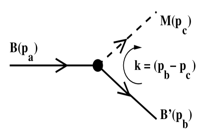
Figure 2: Momentum structure of the strong decay vertex ${\cal M}_{BB^{\prime}M}(k)$ in the initial baryon $B$ center-of-momentum frame.

Based on the lessons learned from earlier work, this calculation includes all allowed combinations of intermediate states $B^{\prime}M$ from the sets

$$M\in\{\pi,K,\eta,\eta^{\prime},\rho,\omega,K^{*}\},\ B^{\prime}\in\{N,\Delta,\Lambda,\Sigma\}.$$ (6)

including all excitations of the baryons states up to and including the $N=3$ band states. Excited mesons states have been omitted at this time as their higher mass and additional angular momentum highly suppresses decays to these states. Studies including more massive initial states should, however, consider including such states.

Based on the range of intermediate states included, it is worth noting that for each $N^{(*)}$ initial state studied, the sum of Eq. 5 ($\sum_{B^{\prime}M}$) includes a total of 591 intermediate baryon-meson states. Similarly, a total of 378 intermediate states are included for each $\Delta^{(*)}$ initial state.

As the self energies due to a given intermediate state depend crucially on the masses adopted for the intermediate hadrons, these are taken to be the physical masses, where known, and model masses [15] otherwise. The ‘bare’ mass required to reproduce the known physical mass of any initial baryon state $B$ considered is found by solving the self-consistent (highly non-linear) equation

$$E+\Sigma_{B}(E)=M_{B}$$ (7)

for the ‘bare’ baryon mass $E_{B}^{0}$. Therefore the integration of Eq. 5 needs to be performed over a range of bare masses $E_{B}$ in order for the final result ($E_{B}^{0}$) to be extracted from the intersection of the left side of Eq. 7 with the right side when $M_{B}=M_{\rm physical}$.

Chapter 2 The Quark Potential Model

The nonrelativistic constituent quark model (NRQM) owes its origin to many authors but the model of Isgur and Karl and collaborators [16, 17, 18, 19] has been qualitatively successful in both meson and baryon sectors, despite its lack of theoretical foundation in QCD. In an effort to correct some of the flaws of the NRQM, the Isgur-Karl model was later ‘relativized’ by Godfrey and Isgur [20] (for mesons) and Capstick and Isgur [21] (for baryons). This latter version has been used by Capstick and Roberts [15, 22, 23] in extensive calculations of strong decay amplitudes. A modified version of this model is used in the present work to obtain the masses and wave functions of known and ‘missing’ baryon states. It is therefore appropriate to give an overview of the main components and discuss the value of some of the parameters used here.

The choice of dynamical degrees of freedom used to represent a baryon depends on momentum transfer. At low $Q^{2}$, they can be taken to be constituent quarks, which are valence quarks with effective masses of about 220 MeV for $u$ and $d$ ($\sim$330 MeV in the NRQM), and about 420 MeV for the $s$ quark ($\sim$550 MeV in the NRQM). In this model the gluon fields affect the quark dynamics by creating a confining potential in which the quarks move. At short distances, a perturbative one-gluon exchange between quarks is assumed to provide the spin-dependent potential.

1 The Hamiltonian

The Hamiltonian used [21] for the baryon system has the form

$$H=H_{0}+V_{\rm oge}+V_{\rm conf}.$$ (1)

where $H_{0}$ is the relativistic kinetic energy term

$$H_{0}=\sum_{i=1}^{3}(p_{i}^{2}+m_{i}^{2})^{1/2},$$ (2)

$V_{\rm oge}$ is the one-gluon-exchange potential, and $V_{\rm conf}$ consists of a string potential and its associated spin-orbit term arising from the Thomas precession.

The one-gluon exchange potential has the form

$$V_{\rm oge}=\sum_{i<j}V_{ij}^{\rm oge}$$ (3)

with the color induced interactions being

$$V_{ij}^{\rm oge}=V_{ij}^{\rm Coulomb}+V_{ij}^{\rm hyperfine}+V_{ij}^{\rm spin-orbit(cm)}$$ (4)

where

$$V_{ij}^{\rm hyperfine}=V_{ij}^{\rm contact}+V_{ij}^{\rm tensor}.$$ (5)

The Coulomb term is spin-independent and proportional to $1/r_{ij}$ (where ${\bf r}_{ij}$ is the relative position of the $(ij)$ quark pair), the spin-orbit and hyperfine interactions are color-magnetic in nature, and the hyperfine interaction consists of a Fermi contact term $\propto\delta^{3}(r_{ij})$ and a tensor piece. The terms of the one-gluon exchange potential can be found from the Breit-Fermi reduction of the one-gluon exchange T-matrix element $\propto\bar{u}({\bf p}^{\prime},s^{\prime})\gamma_{\mu}u({\bf p},s)$ where $u$ is approximated as the Dirac four-spinor of a free particle.

The confining potential is composed of two parts

$$V_{\rm string}=b\sum_{i<j}r_{ij},$$ (6)

and

$$V_{\rm spin-orbit(s)}=\sum_{i<j}V_{ij}^{\rm spin-orbit(Tp)}.$$ (7)

The string part of $V_{\rm conf}$ is the adiabatic potential corresponding to the energy of the minimum-length configuration of the Y-shaped string linking the quarks. The spin-orbit term includes the Thomas precession effects of the full spin-independent potential. For ease of calculation, $V_{\rm string}$ is approximated by a sum of a constant, an effective two-body piece, and a three-body piece

$$V_{\rm string}=C_{qqq}+fb\sum_{i<j}r_{ij}+V_{\rm 3b},$$ (8)

where $C_{qqq}$ is an overall energy shift which arises from the vacuum modifications due to the presence of colored fields in the baryon, $f=0.5493$ is chosen to minimize the size of the expectation value of $V_{\rm 3b}$ in the harmonic oscillator ground state of the baryon system, and $b$ is the meson string tension. The two-body part of $V_{\rm string}$ is calculated directly during the diagonalization of the Hamiltonian, and $V_{\rm 3b}$ is computed perturbatively.

The potentials have been modified from their nonrelativistic limit ($p/m\rightarrow 0$) by several effects. For example, since constituent quarks are not point-like, the interquark coordinate is smeared out over mass-dependent distances. The smearing is brought about by convoluting the potentials with a function

$$\rho_{ij}({\bf r}_{ij})=\frac{\sigma_{ij}^{3}}{\pi^{{\textstyle{3\over 2}}}}e^{-\sigma_{ij}^{2}{\bf r}_{ij}^{2}}.$$ (9)

where the $\sigma_{ij}$ are chosen to smear the interquark coordinate over distances of approximately 0.22 fm for light quarks, and $O(1/M_{Q})$ for heavy quarks $Q$. A second modification allows the potentials to be momentum dependent by introducing factors which replace quark mass terms by energy dependent ones such as

$$\beta_{ij}=1+\frac{p_{ij}^{2}}{(p_{ij}^{2}+m_{i}^{2})^{1/2}(p_{ij}^{2}+m_{j}^{2})^{1/2}}$$ (10)

$$\delta_{ij}=\frac{m_{i}m_{j}}{(p_{ij}^{2}+m_{i}^{2})^{1/2}(p_{ij}^{2}+m_{j}^{2})^{1/2}}$$ (11)

where $p_{ij}$ is the magnitude of the momentum of either quark in the $ij$ center-of-mass frame. These terms are included in the potentials in the form of factors such as $(\delta_{ij})^{1/2+\epsilon_{k}}$ where the $\epsilon_{k}$’s are free parameters designed to allow the rough description of the momentum dependence of each potential.

2 The Parameters

For completeness, we include the final value of some of the relativized quark potential model parameters used in this work. As will be explained in more detail in Chapter 4, the values used in Ref. [21] and subsequent work were not adequate here as they were meant to model a spectrum without taking into consideration the existence of $qqq+q\bar{q}$ configurations. Therefore our work requires slightly different parameters. Another reason for reducing the value of $\sigma_{0}$, which corresponds to the inverse of a quark ‘size’ and is one of the smearing parameters used to define $\sigma_{ij}$ in Eq. 9 (the other parameter being $s$), is that it brings the electromagnetic form factor of the quark required to fit nucleon electromagnetic form factors in relativistic (light-cone based) models more in line with this strong size. Studies have been done with various values of some of the parameters to understand their effects before selecting the final values. Some of the ‘intermediate’ results will be presented in Chapter 4 to illustrate this process. More information about the different potentials, the origin and use of the parameters listed here can be found in Ref. [21] and references within, since their description is beyond the scope of this work.

It is important to note that all spin-orbit effects have been removed from the Hamiltonian used to obtain the wave functions used in this work. Studies on how best to introduce spin-orbit effects are in progress but are secondary to the main goal of this work, and so are not presented at this time.

Table 1: The parameters of the relativized quark potential model.

Parameter	This work	Ref. [21]
${\textstyle{1\over 2}}(m_{u}+m_{d})$ (MeV)	220	Same	Light quark mass
$m_{s}$ (MeV)	419	Same	Strange quark mass
$b$ (GeV2)	0.15	Same	String tension
${\textstyle{1\over 2}}+\epsilon_{\rm cont}$	${\textstyle{1\over 2}}-0.168$	Same	Relativistic factor
${\textstyle{1\over 2}}+\epsilon_{\rm tens}$	${\textstyle{1\over 2}}-0.168$	Same	“
${\textstyle{1\over 2}}+\epsilon_{\rm Coul}$	${\textstyle{1\over 2}}$	Same	“
$\alpha_{s}^{\rm critical}$	0.550	0.60	$\alpha_{s}(Q^{2}=0)$
$\sigma_{0}$(GeV)	0.833	1.80	Relativistic smearing
$s$	1.55	Same	“

Chapter 3 Modeling Strong Decays

1 Introduction

One very important element of our calculation is a model of the momentum dependence of each vertex in Figure 1 (a). If that diagram were to be cut in half, one could see that each half represents a decay $B\rightarrow B^{\prime}M$. We can therefore use a decay model to obtain the structure of the vertex and hence its momentum dependence. The two most suitable classes of models for this work are briefly described below before going into the details of the specific model used here (for a recent review of these and other strong decay models see Ref. [24]).

The first class, known as elementary-meson-emission (EME) models, has baryons treated as objects with a quark structure while mesons are treated as elementary, point-like objects emitted from a quark during the decay. Each decay transition is described in terms of a coupling constant. This implies many parameters, although several coupling constants can be approximately related via SU(2) or SU(3) flavor symmetry. This class of models lends itself well to relativistic treatment, which is often desirable for light mesons such as the pion. Unfortunately since mesons are modeled as point-like objects, treatment of excited mesons is restricted since radial excitations imply an extended spatial wave function which is not modeled.

The other class of models, referred to broadly as pair creation models, treat all hadrons as composite objects. The decay of a hadron coincides with the creation of a quark-antiquark pair somewhere in the hadronic medium. The created antiquark then combines with a quark of the original hadron to create a daughter meson while the created quark becomes part of the other daughter hadron. These models describe hadron emission in a unified way, often involving only one free parameter (the pair-creation strength $\gamma$), and allow for the treatment of all excited baryons and mesons within the same framework. In contrast to EME models, pair creation models are non-relativistic and therefore approximations are made. They are nonetheless more realistic, simple, and have been successfully applied to the study of a broad range of strong decays for both mesons and baryons.

There are several types of pair creation models, such as the ${}^{3}P_{0}$ and ${}^{3}S_{1}$ models (named after the quantum numbers of the created pair), and the flux-tube and string breaking models, where the location of the created pair is restricted to an area inside the chromoelectric flux tube (the tube of gauge field that is shown by lattice QCD to form between two colored sources) or along the string axis. We describe our choice in some detail in the next section.

2 The ${}^{3}P_{0}$ Model

Due to its simplicity and past successful applications to the strong decays of hadrons, the ${}^{3}P_{0}$ model, popularized by Le Yaouanc et al. [25] has been selected to be used in this research. It has been widely applied to baryon decays [15] [22] [23], meson decays, and even generalized to the decay of states composed of n-quarks [26].

Within this model, the strong decay can be seen as a process where a quark-antiquark pair is created from the QCD vacuum with quantum numbers $J^{PC}=0^{++}$. As shown below, in the ${}^{2S+1}L_{J}$ notation, this corresponds to ${}^{3}P_{0}$, hence the name of the model. The pair can be created anywhere in space, but wave function overlaps will naturally strongly suppress creation very far from the initial hadron. The created pair is added to the initial system, giving rise to two new non-interacting final state hadrons. To be observed, these new hadrons must be color singlets. Additionally, the $q\bar{q}$ pair must be neutral with respect to the additive quantum numbers, meaning that it must also be a flavor singlet, and have zero total angular momentum. Because the quark and antiquark have opposite intrinsic parity, parity conservation further dictates the pair be in a relative p-wave (i.e. $L=1$) so that its total spin must be one ($S=1$) to combine to the required $J=0$.

It is important to note that only Okubo-Zweig-Iizuka (OZI) allowed decays are considered, as illustrated in Figure 1(a). A process is said to be OZI-forbidden, or suppressed, [see Figure 1(b)] if the quark of the created quark pair does not combine with quarks in the initial hadron but instead the created quark and antiquark form a separate meson.

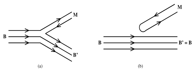
Figure 1: OZI-allowed (a) and suppressed (b) processes $B\rightarrow B^{\prime}M$, in a quark pair creation model.

1 The Operator

The starting point in modeling the $B\rightarrow B^{\prime}M$ transitions of baryons in the ${}^{3}P_{0}$ model is the form of the operator $T$ responsible for the decay. Within this model, the operator does not result from a detailed Hamiltonian that would come from the QCD Lagrangian, as the complexity would be overwhelming. Instead it is entirely phenomenological and is defined only for the decay process under consideration. It has the following form

$$T = -3\gamma\sum_{i,j}\int d{\bf p}_{i}d{\bf p}_{j}\ \delta({\bf p}_{i}+{\bf p}_{j})\ C_{ij}\ F_{ij}\ e^{-f^{2}({\bf p}_{i}-{\bf p}_{j})^{2}}$$ (1)

$$\times \sum_{m}\langle 1,m;1,-m|0,0\rangle\ \chi_{ij}^{m}\ {\cal Y}_{1}^{-m}({\bf p}_{i}-{\bf p}_{j})\ b_{i}^{\dagger}({\bf p}_{i})\ d_{j}^{\dagger}({\bf p}_{j}),$$

where $C_{ij}$ and $F_{ij}$ are the color and flavor wave functions of the created pair, both assumed to be singlet, $\chi_{ij}$ is the spin triplet wave function of the pair, and ${\cal Y}_{1}({\bf p}_{i}-{\bf p}_{j})=|{\bf p}_{i}-{\bf p}_{j}|\ Y_{1}(\widehat{{\bf p}_{i}-{\bf p}_{j}})$ is the solid harmonic indicating that the pair is in a relative p-wave $(L=1)$. Note that the threshold behavior resulting from this $|{\bf p}_{i}-{\bf p}_{j}|$ factor is as seen experimentally. Here $b_{i}^{\dagger}({\bf p}_{i}\/)$ and $d_{j}^{\dagger}({\bf p}_{j}\/)$ are the creation operators for a quark and an antiquark with momenta ${\bf p}_{i}$ and ${\bf p}_{j}$ respectively. The exponential has been introduced to give the vertex a spatial extent by creating the quark-antiquark pair over a smeared region, instead of at a point as is the case in the usual version of the ${}^{3}P_{0}$ model. The addition of this form factor ‘softens’ the vertices and suppresses the self energy contributions from intermediate states where the hadrons have high relative momentum.

There are only two phenomenological parameters in this model. The first one is $\gamma$, the coupling strength, which we fit to the experimentally well known $\Delta\rightarrow N\pi$ decay, and the second one is $f$, which is set to give a reasonable quark-pair-creation vertex size of around 0.35 fm (the same as that used in Geiger and Isgur [10] and Silvestre-Brac and Gignoux [12]).

Consider an initial observable system $A$ (a baryon composed of three quarks) decaying into two observable, non-interacting hadrons; baryon $B$ and meson $C$. One quark from $A$ will merge with the created antiquark to form meson $C$, and the remaining two ‘initial’ quarks will merge with the created quark to form baryon $B$. The notation used is illustrated in Figure 2. Note that in this version of the ${}^{3}P_{0}$ model, quarks 1 and 2 are considered spectators as they do not participate in the decay.

Figure 2: Schematic diagram of the decay $B\rightarrow B^{\prime}M$ in the ${}^{3}P_{0}$ model. The angular momentum notation is shown. The decay proceeds through $B(123)\rightarrow 12(4\bar{4})3\rightarrow B^{\prime}(124)M(\bar{4}3)$.

2 Wave Functions Considerations

For the transition $A\rightarrow BC$, we are interested in evaluating the following transition amplitude

$$M=\langle BC|T|A\rangle,$$ (2)

where $|A\rangle$ denotes the wave function of the initial baryon $A$, and $|BC\rangle$ the wave function of the final baryon-meson pair. The initial system is assumed to be in a static state (made up of a quantum superposition of harmonic oscillator substates), multiplied by a plane wave with relative state momentum ${\bf K}_{a}$ for center-of-mass motion, where $a$ denotes the quantum numbers needed to describe the basis states. The total wave function for the initial state $|A\rangle$ expressed in momentum representation is expanded in terms of basis states $\Psi_{a}^{A}$

$$\Psi^{A,{\bf K}_{a}}=\delta({\bf p}_{a}-{\bf K}_{a})\Psi^{A}=\sum_{a}{d^{A}}_{a}\Psi_{a}^{A,{\bf K}_{a}}.$$ (3)

The coefficients ${d^{A}}_{a}$ are obtained by diagonalization of the Hamiltonian $H$ in the basis of the $\Psi_{a}^{A}$, taken here to be harmonic-oscillator basis states. The series is truncated to $N=2(n_{\rho}+n_{\lambda})+l_{\rho}+l_{\lambda}=6$ for the positive-parity states and $N=7$ for negative-parity states, giving of the order of 100 substates for each $J^{P}$. Note that the level $N$ of the expansion is related to the sum of the powers of the two coordinates $\rho$ and $\lambda$ (see Appendix 6) in the associated Laguerre polynomials. A higher power means a shorter length scale, therefore the maximum $N$ was chosen to ‘resolve’ the shortest range interaction in the Hamiltonian, or equivalently allow the variational calculation of the energy to converge. The expansion coefficients $d_{a}^{A}$ are such that the total wave function $\Psi^{A,{\bf K}_{a}}$ is antisymmetric, despite the fact that the basis states $\Psi_{a}^{{\bf K}_{a}}$ are taken to be antisymmetric only in the first two quarks.

The wave functions for the final baryon and meson are given in a similar fashion

$$\Psi^{B,{\bf K}_{b}}=\delta({\bf p}_{b}-{\bf K}_{b})\Psi^{B}=\sum_{b}d_{b}^{B}{\Psi_{b}^{B,{\bf K}_{b}}}.$$ (4)

$$\Psi^{C,{\bf K}_{c}}=\delta({\bf p}_{c}-{\bf K}_{c})\Psi^{C}=\sum_{c}d_{c}^{C}\Psi_{c}^{C,{\bf K}_{c}}.$$ (5)

By combining $\Psi^{B,{\bf K}_{b}}$ and $\Psi^{C,{\bf K}_{c}}$ we obtain a wave function $|BC;J_{b}M_{b}{\bf K}_{b}J_{c}M_{c}{\bf K}_{c}\rangle$ which describes the hadrons in a plane wave with their angular momenta decoupled. For ease in further treatment of angular momenta, we couple ${\bf J}_{b}+{\bf J}_{c}={\bf J}_{bc}$, and change the variables ${\bf p}_{b}$ and ${\bf p}_{c}$ to ${\bf K}={\bf p}_{b}+{\bf p}_{c}$ and ${\bf k}={\textstyle{1\over 2}}({\bf p}_{b}-{\bf p}_{c})$. Then ${\bf K}$ represents the total momentum of the $BC$ system and is conserved through the term $\delta({\bf p}_{a}-{\bf K}_{a})$ of equation 3, and ${\bf k}$ is the relative momentum between $B$ and $C$. Instead of using a plane wave $|{\bf k}\rangle$, we change to a spherical wave $|lmk\rangle$ via

$$\langle{\bf p}_{b}{\bf p}_{c}|{\bf K}_{0}lmk_{0}\rangle=\delta({\bf K}-{\bf K}_{0})\frac{{Y^{m}}_{l}(\bf\hat{k})}{k^{2}}\delta(k-k_{0}).$$ (6)

Finally, the relative momentum $l$ is coupled to $J_{bc}$ to give the total angular momentum $J_{a}$, so that the form of the final state wave function becomes

$$|BC,J_{b}J_{c},J_{bc}l;J_{a}M_{a};{\bf K}_{0}k_{0}\rangle$$ (7)

$$= \int d{\bf K}_{b}d{\bf K}_{c}\sum_{M_{bc},m,M_{b},M_{c}}\langle J_{b}M_{b}J_{c}M_{c}|J_{bc}M_{bc}\rangle$$

$$\times\langle J_{bc}M_{bc}lm|J_{a}M_{a}\rangle\langle{\bf K}_{b}{\bf K}_{c}|{\bf K}_{0}lmk_{0}\rangle|BC,J_{b}M_{b}{\bf K}_{b}J_{c}M_{c}{\bf K}_{c}\rangle.$$

Baryon states are written as

$$\Psi=C_{A}\phi\sum\psi\chi.$$ (8)

where $C_{A}$, $\phi$, $\psi$, and $\chi$ are the color, flavor, spatial, and spin wave functions respectively. The baryon wave functions used in this calculation were produced using a relativized model [21] with variable-strength spin-dependent (one-gluon exchange) contact, tensor, and spin-orbit interactions between the quarks. More details about the baryon wave functions can be found in Appendix 6.

3 Transition Amplitude

From equation 1, the transition amplitude is not Galilean invariant since it contains a factor $\delta{\bf p}$, where ${\bf p}$ is evaluated in a definite frame. The results therefore depend on the chosen frame of reference. A good choice of frame is the one where the decaying baryon $A$ is at rest, so we set ${\bf K}_{a}=0$. Momentum conservation yields a factor $\delta({\bf K}_{0})$ in the amplitude, and we now rewrite equation 2 as

$$\langle BC|T|A\rangle=\delta({\bf K}_{0})M_{A\rightarrow BC}.$$ (9)

Incorporating equations 3, 4, and 5, we obtain the expression

$$M_{A\rightarrow BC}=\sum_{a,b,c}d_{b}^{B*}d_{c}^{C*}d_{a}^{A}M_{A\rightarrow BC}(a,b,c)$$ (10)

The color, flavor, spin, and spatial degrees of freedom can be separated via invariance techniques. The resulting amplitude then reduces to products of sums over internal summation variables of $6-j$ and $9-j$ coefficients from angular momentum recoupling, and flavor, and spatial matrix elements that can be calculated independently, which then can be combined to give a total decay matrix element. The final form of $M_{A\rightarrow BC}(a,b,c)$ is

$$M_{A\to BC}(a,b,c)={6\gamma\over 3\sqrt{3}}(-1)^{J_{a}+J_{b}+\ell_{a}+\ell_{b}-1}\sum_{J_{\rho},s_{a},s_{b}}{\hat{J}}\/_{\rho}^{2}\hat{s}_{a}{\hat{S}}\/_{a}{\hat{L}}\/_{a}\hat{s}_{b}{\hat{S}}\/_{b}{\hat{L}}\/_{b}$$

$$\left\{\matrix{S_{a}&L_{\rho}&s_{a}\cr\ell_{a}&J_{a}&L_{a}\cr}\right\}\left\{\matrix{L_{\rho}&S_{\rho}&J_{\rho}\cr{1\over 2}&s_{a}&S_{a}}\right\}\left\{\matrix{S_{b}&L_{\rho}&s_{b}\cr\ell_{b}&J_{b}&L_{b}\cr}\right\}\left\{\matrix{L_{\rho}&S_{\rho}&J_{\rho}\cr{1\over 2}&s_{b}&S_{b}}\right\}$$

$$(-1)^{\ell+\ell_{a}+J_{c}-L_{c}-S_{c}}{\cal F}(ABC)$$

$$\times\sum_{S_{bc}}(-1)^{s_{a}-S_{bc}}\left[\matrix{J_{\rho}&{\textstyle{1\over 2}}&s_{b}\cr{\textstyle{1\over 2}}&{\textstyle{1\over 2}}&S_{c}\cr s_{a}&1&S_{bc}}\right]\sum_{L_{bc}}(-1)^{L_{bc}}\left[\matrix{s_{b}&\ell_{b}&J_{b}\cr S_{c}&L_{c}&J_{c}\cr S_{bc}&L_{bc}&J_{bc}}\right]$$

$$\times\sum_{L}{\hat{L}}\/^{2}\left\{\matrix{s_{a}&\ell_{a}&J_{a}\cr L&S_{bc}&1}\right\}\left\{\matrix{S_{bc}&L_{bc}&J_{bc}\cr\ell&J_{a}&L}\right\}\varepsilon(\ell_{b},L_{c},L_{bc},\ell,\ell_{a},L,k_{0}),$$ (11)

where the factor of $6$ comes from the redefinition, for the created pair, ${\bf P}={\bf p}_{i}+{\bf p}_{j}$ and ${\bf p}={\textstyle{1\over 2}}({\bf p}_{j}-{\bf p}_{i})$ so that the spherical harmonic found in the operator (eq. 1) can be rewritten as $-3\gamma{\cal Y}_{1}(-2{\bf p})=6\gamma{\cal Y}_{1}({\bf p})$. The overall factor of $\frac{1}{3}$ is the color matrix element, ${\cal F}$ is the flavor overlap, and $\varepsilon$ is the spatial matrix element.

Further explanation of notation and derivations of some components have been gathered in appendix 7 for the interested reader.

Chapter 4 Results

Graphical and tabulated results for the self energies of the ground state Nucleon, $\Delta$ and non-strange $L=1$ negative-parity states are presented in the following sections. First, evidence of the convergence of our results is shown, indicating that a minimum number of intermediate states have been included in order to obtain stable and reliable results. The same graphs also show the effects of the various decay thresholds, and their effect on the sums of self energies. Next, tables displaying the impact of changes in the Hamiltonian and the associated baryon model wave functions are presented. Finally the $qqq$ spectrum obtained from the modified Hamiltonian is graphically compared with the spectrum of bare energies obtained from fitting the sum of the bare energies and self energies to the physical masses. This illustrates that it is possible, in a self-consistent calculation, to describe the observed masses with a combination of splittings induced by interquark forces and differences in the self energies.

1 Convergence and Thresholds

One important result coming out of this calculation is the phenomenon of convergence. As pointed out before, the number and type of intermediate states included in this type of calculation can dramatically change the final results. In the figures that follow, this concept and the associated consequences will be illustrated for the states studied.

Figures 1 through 6 show the self-energy contributions to the masses of several baryons, from the sum of intermediate $B^{\prime}M$ states for $B^{\prime}$ including progressively higher harmonic oscillator bands, and $M$ the complete set of pseudo-scalar and vector mesons (i.e. $\pi,K,\eta,\eta^{\prime},\rho,\omega,K^{*}$). These figures show the results obtained from using wave functions created from a Hamiltonian that includes both the contact and the tensor part of the hyperfine interaction. In each figure, each line represents the sum $E+\Sigma_{B}(E)$ with $\Sigma_{B}(E)$ obtained with a set of baryons $B^{\prime}$ in the harmonic oscillator bands indicated in the subscript [$\Sigma(E)_{N=0}$, $\Sigma(E)_{N\leq 1}$, $\Sigma(E)_{N\leq 2}$, and $\Sigma(E)_{N\leq 3}$]. For each of these sums of intermediate states, the corresponding bare mass $E_{B}^{0}$ can be extracted by reading the value of the energy $E$ corresponding to the intersection between the curve for the sum of self energies $E+\Sigma_{B}(E)$ and the horizontal line representing the physical mass. This process is in effect solving

$$E+\Sigma_{B}(E)=M_{B},$$ (1)

for $E=E_{B}^{0}$ when $M_{B}=M_{\rm physical}$ with progressively larger sum over bands of baryon intermediate states $N=0$, $N\leq 1$, $N\leq 2$, and $N\leq 3$.

As will be seen in some of the figures and tables that follow, occasionally more than one solution is possible for Eq. 1 due to oscillations caused by the presence of $B^{\prime}M$ decay thresholds (the energies at which the decays $B\rightarrow B^{\prime}M$ become physical, i.e. energetically possible). In these few cases a range of values is presented unless it is clear that one solution is favored. More details are presented in the next section.

1 Nucleon and Delta Ground States

Figure 1 and Table 3(b) show the self energy contributions to the mass of the Nucleon from a progressively larger sum of intermediate baryon-meson states. The first point to notice is the sizeable difference between the ‘bare mass’ $E_{B}^{0}$ when only baryons in the $N=0$ band are included, i.e. $E_{B}^{0}=1.85$ GeV, and when other baryon states are included, $E_{B}^{0}=2.36$ to $2.50$ GeV. These bare masses are not observables, but the mass splitting between the nucleon and other states is, therefore any large variation in the bare mass of the nucleon can change its relationship with other states in the spectrum.

Next note that this ‘bare mass’ difference is not ‘built’ of equal contributions from each set of intermediate states but comes mostly from the inclusion of the $N=0$ and $N=1$ states (first band of negative-parity excited states), indicating that the ground state nucleon couples more strongly to states in these bands. Here the $N=0$ line can be thought of as a starting point for this work, since the best of the previous studies of this state include only the intermediate states included in this band, or restricted the intermediate mesons to only the pion. The addition of the $N=2$ and $N=3$ bands of states changes the bare mass by a very small amount indicating that the sum over intermediate states has converged and a stable solution has been reached for the ground state nucleon. This is a very important result, and it will be shown that a lack of convergence can greatly affect the final results of such calculations. As will be seen below, the impact of the different bands of states varies with the initial state studied, and the inclusion of the $N=2$ and $N=3$ band baryons is important for other states. In the case of the nucleon, these bands were added for consistency.

An additional item that needs explanation is the presence of multiple solutions for Eq. 1 when all intermediate baryon states up to the $N=3$ harmonic oscillator band are included (solid line in Figure 1). This stems from the presence of decay thresholds and their effect on the size of the self energies. The locations of some ground state thresholds are labeled on the figure, but others cannot be identified due to the large number of $B^{\prime}M$ states included. It is possible that these threshold effects could be ‘dampened’ by the inclusion of the widths of intermediate particles as an imaginary part in the energy denominator of Eq. 5, but that is a higher-order effect which remains to be investigated. In selecting a favored solution for the nucleon, studies of the dependence of its self energy on the wave functions have shown that the second and third solutions sometimes vanish, but the first solution is always present. Therefore it seems prudent to retain only the lower bare mass for the nucleon until more consistent results are obtained for the other masses.

Figure 1: Sum of the bare energy and self energies as a function of the bare energy for the Nucleon ground state with $\alpha_{s}=0.55$ and $\alpha=0.5$ GeV.

Figure 2 and Table 3(b) show similar results for the ground state $\Delta$. Again the evolution of the bare masses is clear and once more the $N=0$ and $N=1$ band baryon states are seen to make the largest contributions to the self energies. Here the convergence is even more apparent, as the addition of the $N=2$ and $N=3$ band states only resulted in an overall downward shift of the $E+\Sigma_{B}(E)$ curves with very little movement along the energy axis. The almost vertical slope of the last three lines clearly indicates that not only has the sum over intermediate states converged, but that the inclusion of additional states would have an insignificant impact on the final bare mass.

Note that the importance of the labeled thresholds in the case of the $\Delta$ is different than those for the nucleon, revealing some of the differences in the internal structure of these two states. This reflects the results of similar strong decay calculations which predict where to look experimentally for resonances by highlighting strong coupling to certain decay channels over others. These calculations also explain why some resonances remain ‘missing’; they couple weakly to experimentally accessible decay channels.

Figure 2: Sum of the bare energy and self energies as a function of the bare energy for the $\Delta$ ground state with $\alpha_{s}=0.55$ and $\alpha=0.5$ GeV.

Combination of the results of Figures 1 and 2 [also see Table 3(b)] shows that if only intermediate ground state baryons ($N=0$ band) are included, the $N$-$\Delta$ splitting is roughly $290$ MeV. When states in the $N=1$ band are included the splitting is reduced to about $140$ MeV, and that result remains mostly unchanged by the addition of baryon intermediate states in the $N=2$ and $N=3$ bands. This agrees well with the expectation from other models (see Ref. [27] where the authors find that within their model, 2/3 of the $N$-$\Delta$ mass splitting comes from one-gluon exchange effects, with the remaining third coming from pion-exchange) that a substantial portion of the $N$-$\Delta$ splitting should come from a source other than the quark-quark residual interactions, in this case a difference in self energies due to all $B^{\prime}M$ intermediate states. This result will be shown to hold despite changes to the wave functions from variations in the quark residual interactions.

2 Non-Strange $L=1$ Negative-Parity Baryons

The results for the $L=1$ negative-parity states are presented in Figures 3 through 6 and Table 3(b). States with same quantum numbers are shown together to facilitate comparisons.

Figure 3: Sum of the bare energy and self energies as a function of the bare energy for a) $N{\textstyle{1\over 2}}^{-}(1535)$ and b) $N{\textstyle{1\over 2}}^{-}(1650)$ with $\alpha_{s}=0.55$ and $\alpha=0.5$ GeV.

Figure 3 shows the results for the spin-partner $N{\textstyle{1\over 2}}^{-}$ states. It can immediately be seen that the bands of intermediate states have a different impact on these states (and in fact on all the $L=1$ negative-parity states) compared to the situation with the Nucleon and $\Delta$ shown above. Here, intermediate baryon states up to the $N=2$ band make sizeable contributions but $N=3$ states only change the results marginally. This indicates that the results have converged and that all intermediate baryons up to and including the $N=2$ band states are required for convergence.

If only ground-state baryons are included, the splitting between the two $N{\textstyle{1\over 2}}^{-}$ states can be seen to be roughly 20 MeV, while it can be observed to grow to roughly 100 MeV with the inclusion of the $N=1$ band baryons. Further addition of the $N=2$ and $N=3$ band states brings convergence and closes this gap to about 5 MeV. This illustrates the wide difference in results that can be obtained if the set of intermediate states is not large enough to attain convergence.

Figure 4: Sum of the bare energy and self energies as a function of the bare energy for a) $N{\textstyle{3\over 2}}^{-}(1520)$ and b) $N{\textstyle{3\over 2}}^{-}(1700)$ with $\alpha_{s}=0.55$ and $\alpha=0.5$ GeV.

Figure 4 shows similar results for the $N{\textstyle{3\over 2}}^{-}$ pair. Again the splitting between these states induced by these self-energy effects varies from 25 MeV to 170 MeV depending on number of intermediate states included. Note that in the case of the $N{\textstyle{3\over 2}}^{-}(1520)$, although the $N=3$ band intermediate states were not required for convergence, addition of these states resolved the multiple solution problem. This validates the considerable extra effort required to include such a large number of intermediate states. Note again the differences in the threshold pattern between the two states hinting at how differently these states couple to the various intermediate states.

Figure 5: Sum of the bare energy and self energies as a function of the bare energy for a) $\Delta{\textstyle{1\over 2}}^{-}(1620)$ and b) $\Delta{\textstyle{3\over 2}}^{-}(1700)$ with $\alpha_{s}=0.55$ and $\alpha=0.5$ GeV.

Figures 5 and  6 complete the set of non-strange $L=1$ negative-parity baryon states with the $\Delta{\textstyle{1\over 2}}^{-}(1620)$, $\Delta{\textstyle{3\over 2}}^{-}(1700)$, and $N{\textstyle{5\over 2}}^{-}(1675)$ states. The two $\Delta$ states could actually be seen to be split by a fair amount if only the $N=0$ and $N=1$ band intermediate states are included, in a way mimicking spin-orbit splitting. However, with the addition of the other two bands of states, the $\Delta(1620)$, which was up to that point much lighter than its spin partner, becomes almost degenerate with the $\Delta(1700)$ and even heavier by roughly 12 MeV. Of course these are states that are known to be affected strongly by spin-orbit interactions between the quarks (which are not included in this work), so the ordering is, at this time, inconclusive. This stresses once again the impact of the choice of intermediate states on the final results. Since the graphs show robust results, we are confident that, for this model, the final ordering is the correct one prior to the inclusion of spin-orbit effects.

Figure 6: Sum of the bare energy and self energies as a function of the bare energy for $N{\textstyle{5\over 2}}^{-}(1675)$ with $\alpha_{s}=0.55$ and $\alpha=0.5$ GeV.

3 $N=2$ Band States

Figure 7: Sum of the bare energy and self energies as a function of the bare energy for $N{\textstyle{1\over 2}}^{+}(1440)$ with $\alpha_{s}=0.55$ and $\alpha=0.5$ GeV.

Finally, to illustrate a case where convergence is not yet achieved, Figure 7 is included to show the results for the Roper resonance $N{\textstyle{1\over 2}}^{+}(1440)$, with these same set of intermediate states. Not only do we not have a unique solution, but it is clear from the difference between the bare mass for $N\leq 2$ and $N\leq 3$ baryon intermediate states included in the sum that the addition of more intermediate states could significantly change the final result. This indicates the need to extend the summation over intermediate states to include at least $N=4$ band positive parity baryon states. Note that the effect of the $N=1$ band intermediate states is minimal, in contrast to the different situations shown earlier. As expected, this indicates that as states from higher harmonic oscillator bands are studied, inclusion of a large set of intermediate states will be required, with a decreased impact of the lower band states and an increased impact of the higher band states.

2 Hamiltonian vs. Self Energies

As mentioned previously, the splittings between the states resulting from the differences in self energies are expected to be comparable in size to those that arise from residual interactions between quarks. As a consequence, a self-consistent calculation requires that those interactions be adjusted, and with them the wave functions, to account for the additional splittings. A priori, we do not know how to modify the Hamiltonian to get the desired result of agreement between the bare energies and the modified $qqq$ spectrum, as each term affects both the model masses and the baryon wave functions. The latter affect the corresponding strong decay matrix elements and hence the size of the self energies. To better understand this process, the splittings of the states under consideration are examined using several different values of the parameters listed in Table 1. Since the best value of the ${}^{3}P_{0}$ decay strength parameter $\gamma$ is affected by changes in the wave functions, it was refitted each time to reproduce the strength of the $\Delta\rightarrow N\pi$ decay calculated with the model of Ref [15]. Additionally, the harmonic oscillator parameter $\alpha$ is chosen on a coarse grid to be such that the masses are roughly minimized, with the ground state $\Delta$ being at or near its physical mass.

Four different cases are presented below; first, all quark-quark residual interactions are turned off leaving only the confining potential to act between quarks; second, the contact part of the one-gluon exchange hyperfine interaction is included but at about half the strength of the value used in Ref. [15]. Note that although the value of $\alpha_{s}$ is only marginally lower (see Table 1), lowering the value of $\sigma_{0}$ has the effect of increasing the size of the quarks thereby reducing the strength of short-range interactions. In the last two cases, the tensor part is also included (proportionally to the contact interaction) and results are presented for two different values of the oscillator parameter $\alpha$. Each table shows the experimental masses of the states, the model mass obtained from diagonalisation of the Hamiltonian, and the bare masses, extracted from graphs similar to those presented above, solving Eq. 1 for progressively larger sums of intermediate states. The presence of multiple solutions is indicated by a range of energies, or an additional value in parentheses when one answer was favored.

Table 1: Bare masses (GeV) for $\alpha_{s}=0.0$ and $\alpha=0.4$ GeV, no residual quark interactions.

State	Model	$N=0$	$N\leq 1$	$N\leq 2$	$N\leq 3$
(Expt. Mass)	Mass
$[N{\textstyle{1\over 2}}^{+}](0.938)$	1.230	1.858	2.358	2.367	2.387-2.492
$[\Delta{\textstyle{3\over 2}}^{+}](1.232)$	1.232	2.132	2.508	2.525	2.538
$[N{\textstyle{1\over 2}}^{-}](1.535)$	1.545	1.762	2.500	2.767	2.783
$[N{\textstyle{1\over 2}}^{-}](1.650)$	1.546	1.800	2.487	2.767	2.783
$[\Delta{\textstyle{1\over 2}}^{-}](1.620)$	1.546	1.812	2.467	2.767	2.787
$[N{\textstyle{3\over 2}}^{-}](1.520)$	1.546	1.758	2.400	2.787	2.800
$[N{\textstyle{3\over 2}}^{-}](1.700)$	1.547	1.850	2.537	2.767	2.783
$[\Delta{\textstyle{3\over 2}}^{-}](1.700)$	1.546	2.037	2.550	2.878	2.800
$[N{\textstyle{5\over 2}}^{-}](1.675)$	1.547	2.042	2.525	2.800	2.817

When wave functions with no residual quark-quark interactions are used to calculate the self energies, this results in the range of bare masses shown in Table 1. As can be expected, model states are mostly degenerate but this still results in a splitting between the ground state $N$ and $\Delta$ of about 150 MeV due to the difference in self energies from the $B^{\prime}M$ loops. This splitting comes from flavor and spin structure differences between those states, and from differences in how each state couples to the various intermediate states included in the sum. It was verified that if the masses of all baryons and mesons are assumed to be degenerate, and only ground state intermediate baryons are included in the sum, the splitting between the $N$ and $\Delta$ ground states disappears, thereby verifying in this model Żenczykowski [6]’s statement about the minimum number of intermediate baryon and meson states to be included to reach this symmetry limit.

Table 2: Bare masses (GeV) for $\alpha_{s}=0.55$, $\alpha=0.4$ GeV, with hyperfine contact interactions only.

State	Model	$N=0$	$N\leq 1$	$N\leq 2$	$N\leq 3$
(Expt. Mass)	Mass
$[N{\textstyle{1\over 2}}^{+}](0.938)$	1.081	1.812	2.342	2.358	2.375
$[\Delta{\textstyle{3\over 2}}^{+}](1.232)$	1.232	2.112	2.500	2.508	2.533
$[N{\textstyle{1\over 2}}^{-}](1.535)$	1.505	1.742	2.108	2.775	2.787
$[N{\textstyle{1\over 2}}^{-}](1.650)$	1.588	1.787	2.475	2.750	2.758
$[\Delta{\textstyle{1\over 2}}^{-}](1.620)$	1.568	1.787	2.200(2.425)	2.775	2.787
$[N{\textstyle{3\over 2}}^{-}](1.520)$	1.505	1.750	2.0625	2.612	2.700-2.787
$[N{\textstyle{3\over 2}}^{-}](1.700)$	1.588	1.787	2.358(2.512)	2.758	2.775
$[\Delta{\textstyle{3\over 2}}^{-}](1.700)$	1.568	2.033	2.358(2.525)	2.787	2.792
$[N{\textstyle{5\over 2}}^{-}](1.675)$	1.588	2.037	2.100(2.500)	2.733(2.775)	2.787

Table 2 shows the changes created by the inclusion of the contact part of the hyperfine interaction (with no tensor or spin-orbit interactions). As mentioned above, the contact interaction is roughly half the strength of that used in Ref. [15] and the following papers. In the model, the degeneracy is now lifted between the spin partners $N$-$\Delta$, the $N{\textstyle{1\over 2}}^{-}$ states, and $N{\textstyle{3\over 2}}^{-}$ states. Interestingly, the spin-orbit partners $\Delta{\textstyle{1\over 2}}^{-}$ and $\Delta{\textstyle{3\over 2}}^{-}$ states remain degenerate. Note that spin-orbit interactions are not included in their wave functions. It is important to note that after the addition of all intermediate $B^{\prime}M$ states, the $N$-$\Delta$ splitting remains roughly 150 MeV, demonstrating a stable result for these states. Note also that the ordering of the $N{\textstyle{1\over 2}}^{-}$ states is seen to change as more intermediate states are added, emphasizing the point that not all relevant effects have been included by previous calculations which include only $N=0$ intermediate states.

Table 3: Bare masses (GeV) for $\alpha_{s}=0.55$ with hyperfine contact and tensor interactions.

a) $\alpha=0.4$ GeV.

State	Model	$N=0$	$N\leq 1$	$N\leq 2$	$N\leq 3$
(Expt. Mass)	Mass
$[N{\textstyle{1\over 2}}^{+}](0.938)$	1.082	1.812	(2.175)2.342	2.358	2.375
$[\Delta{\textstyle{3\over 2}}^{+}](1.232)$	1.232	2.112	(2.358)2.500	2.508	2.525
$[N{\textstyle{1\over 2}}^{-}](1.535)$	1.500	1.745	2.105	2.712	2.735
$[N{\textstyle{1\over 2}}^{-}](1.650)$	1.572	1.783	2.412	2.737	2.758
$[\Delta{\textstyle{1\over 2}}^{-}](1.620)$	1.570	1.783	2.200(2.412)	2.725(2.775)	2.787
$[N{\textstyle{3\over 2}}^{-}](1.520)$	1.506	1.750	2.062	2.600	2.650-2.785
$[N{\textstyle{3\over 2}}^{-}](1.700)$	1.606	1.787	2.350(2.512)	2.775	2.812
$[\Delta{\textstyle{3\over 2}}^{-}](1.700)$	1.569	2.375	2.350(2.530)	2.787	2.795
$[N{\textstyle{5\over 2}}^{-}](1.675)$	1.584	2.037	2.100(2.492)	2.787	2.800

b) $\alpha=0.5$ GeV.

State	Model	$N=0$	$N\leq 1$	$N\leq 2$	$N\leq 3$
(Expt. Mass)	Mass
$[N{\textstyle{1\over 2}}^{+}](0.938)$	1.082	1.850	2.367	2.375	2.392(2.500)
$[\Delta{\textstyle{3\over 2}}^{+}](1.232)$	1.232	2.137	2.508	2.517	2.537
$[N{\textstyle{1\over 2}}^{-}](1.535)$	1.500	1.762	2.375	2.737	2.758
$[N{\textstyle{1\over 2}}^{-}](1.650)$	1.572	1.783	2.475	2.742	2.762
$[\Delta{\textstyle{1\over 2}}^{-}](1.620)$	1.570	1.800(2.025)	2.467	2.800	2.812
$[N{\textstyle{3\over 2}}^{-}](1.520)$	1.506	1.762	2.082(2.367)	2.637(2.793)	2.800
$[N{\textstyle{3\over 2}}^{-}](1.700)$	1.606	1.787	2.537	2.812	2.825
$[\Delta{\textstyle{3\over 2}}^{-}](1.700)$	1.569	2.050	2.558	2.787	2.800
$[N{\textstyle{5\over 2}}^{-}](1.675)$	1.584	2.050	(2.100)2.512	2.787	2.800

Tables 3 show the results (previously illustrated in Figures 1 through 6) when both the contact and tensor parts of the hyperfine interaction are included in the Hamiltonian. Here the tensor interaction has the strength required from a consistent nonrelativistic limit of one-gluon exchange. Each table reflects a different value of the harmonic oscillator parameter $\alpha$ (0.4 and 0.5 GeV). Again the $N$-$\Delta$ splitting is unaffected by the changes, as the wave functions for these two states are essentially unchanged by this change in the basis states. The splittings in the bare masses of other states are not strongly affected by the change in $\alpha$. The model masses are minimized with a value of $\alpha=$0.5 GeV, so the results using this basis are preferred.

3 The Spectrum

Finally this section is brought to a close with the presentation of three figures showing the progression of the relationship between the model masses and the bare masses required to reproduce the masses of the states extracted from data analyses. In each figure the two different mass scales have been adjusted so that the bare and model masses of the ground state $\Delta$ coincide. The bare masses shown include all intermediates $B^{\prime}M$ states for each set of parameters.

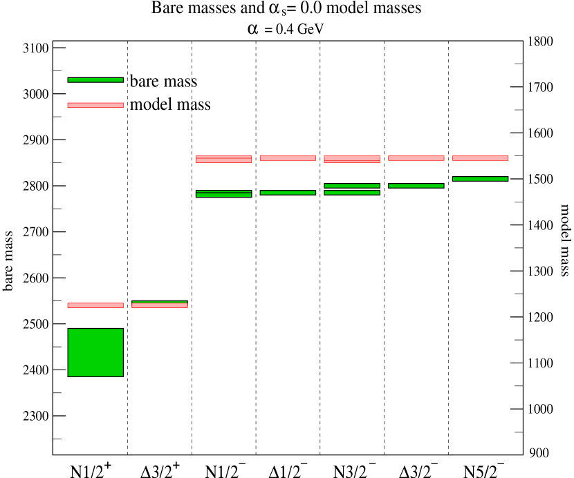
Figure 8: Comparison of the spectra of the bare masses required to fit the physical masses of the states shown and model masses obtained from a Hamiltonian with no residual quark-quark interactions. Here $\alpha_{s}=0.0$ and $\alpha=0.4$ GeV.

When all residual interactions between quarks have been removed, the spectrum of the states studied appears as shown in Figure 8. As stated above and seen here, model masses are degenerate by oscillator band. The inclusion of self energy loops requires different bare energies to fit the physical masses of the $N$ and $\Delta$ ground states, and reduces the splitting in the bare energies between oscillator bands. The Hamiltonian therefore produces model masses in bands that are too far apart at this point.

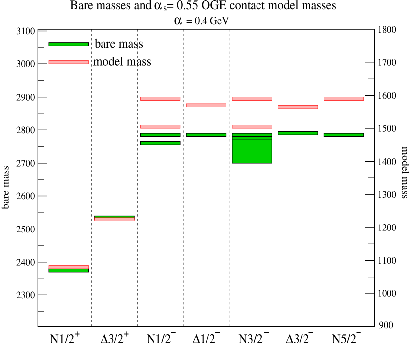
Figure 9: Comparison of the spectra of the bare masses required to fit the physical masses of the states shown and model masses obtained from a Hamiltonian with hyperfine contact interactions only. Here $\alpha_{s}=0.55$ and $\alpha=0.4$ GeV.

As seen in Figure 9, the addition of reduced-strength contact interactions between quarks induces configuration mixing in the wave functions and lifts the degeneracy between spin partners. States split by other type of interactions remain mostly unchanged by this addition. The effect of the self energies on the bare masses extracted from the physical masses also changes, although the $N$-$\Delta$ bare mass splitting is stable at roughly 150 MeV. The order of the two $N{\textstyle{1\over 2}}^{-}$ states, on the other hand, is reversed with the bare mass of the predominantly spin-1/2 state heavier than that of the predominantly spin-3/2 state, and the splitting is larger. The splitting between the bare masses of $N{\textstyle{3\over 2}}^{-}$ states appears to be reduced by the inclusion of loops but the presence of multiple solutions blurs the picture somewhat.

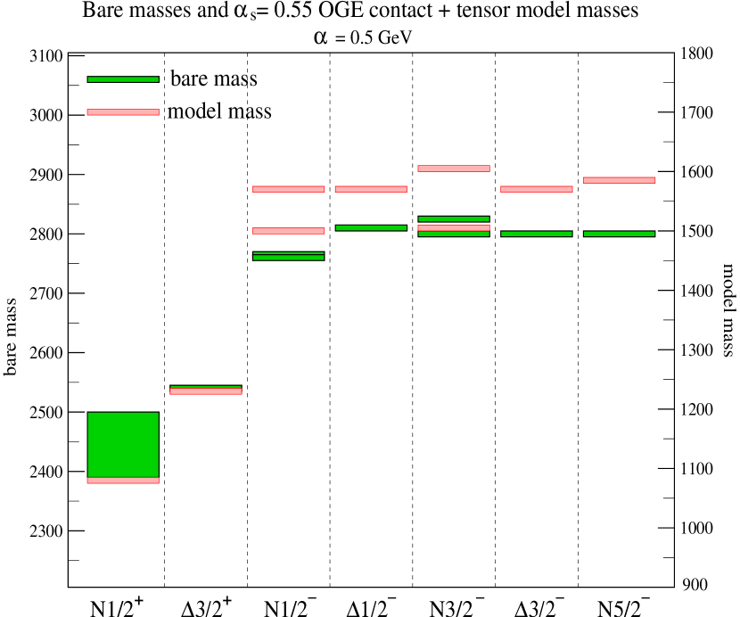
Figure 10: Comparison of the spectra of the bare masses required to fit the physical masses of the states shown and model masses obtained from a Hamiltonian with hyperfine contact and tensor interactions. Here $\alpha_{s}=0.55$ and $\alpha=0.5$ GeV.

The addition of the tensor part of the hyperfine interaction changes the spectra once again, as shown in Figure 10. The modifications to the Hamiltonian close slightly the splitting between the model masses of the $N{\textstyle{1\over 2}}^{-}$ states, and open it for the $N{\textstyle{3\over 2}}^{-}$ states. On the other hand the required bare energies of the $N{\textstyle{1\over 2}}^{-}$ states are almost degenerate, and those of the $N{\textstyle{3\over 2}}^{-}$ states are separated by about 25 MeV. It is expected that the mixing between states with same quantum numbers due to self energy loops will widen the gaps in both cases, so this picture is not yet complete. The splitting between oscillator bands is still larger for the model spectrum than for the bare mass spectrum but the overall agreement between the spectra remains fairly good.

In closing, it is important to mention the extensive computational work required to obtain the results presented in this Chapter and which comprised the most time consuming part of this work. The code used to produce the analytical form of the momentum dependence of the strong decay vertices was entirely done using the symbolic manipulator Maple. The code is based on the general method of Roberts and Silvestre-Brac [26] and was thoroughly tested by reproducing the large number of decay amplitudes found in several published papers by Capstick and Roberts [15, 22, 23]. The analytical expressions produced by the Maple code were subsequently translated into the programming language C, and then included in the code which numerically calculates the principal part of the loop integration using algorithms such as Gauss-Laguerre and Gauss-Legendre quadratures. These extensive calculations would not have been possible without access to the FSU Physics Department Computing Cluster. The computational time currently required to obtain the results listed in just one of the tables presented above is of the order of 5 days of full-time computing for an average of 10 nodes in the cluster. This does not, however, reflect the many months of intensive computing work done prior to this ‘step’ when several of the analytical components of the decay amplitudes were computed and stored. The interested reader is referred to Appendix 8 for more details about the computational methods used during this project.

Chapter 5 Conclusion

Within the context of the relativized quark model, a comprehensive study has been carried out of the effects of baryon-meson intermediate states, in the form of self-energy loop corrections to the mass of several baryons. The baryon states whose self energies have been studied include the nucleon and Delta ground states and the first band of negative-parity excited baryons. The ${}^{3}P_{0}$ decay model is used to obtain the analytical form of the momentum dependence of the baryon-baryon-meson vertices needed in the loop calculations. The model is modified to take into account the size of the constituent-quark pair-creation vertex. Wave functions generated from a Hamiltonian including reduced-strength one-gluon-exchange interactions between quarks are used to calculate the self energies. Since masses play a crucial role in the size of the self energies, physical masses are used where known, and model masses [15] used otherwise, for the intermediate baryons and mesons. The bare energy of the initial baryon is determined self-consistently by calculating the self energies for a range of bare energies, then finding the solution to Eq. 1 when $M_{B}=M_{\rm physical}$ for each initial baryon studied.

As demonstrated by Żenczykowski [6], a minimum set of baryon-meson intermediate states is required to recover the SU(3)${}_{f}\times$SU(2)_spin symmetry limit, while Brack and Bhaduri [9] showed that intermediate baryon states up to at least the second band ($N=3$) of negative-parity excited states must be included in order for the sum over intermediate baryon-meson states to converge. It is clear that truncation at only ground state baryons or only pseudo-scalar mesons leads to physically meaningless results. The present work therefore uses for the first time a complete set of spin-flavor symmetry related baryon-meson intermediate states, while at the same time including excited baryon states up to the $N=3$ band, to insure the convergence of the sum of intermediate states. It is shown that drastically different answers are obtained for some states if this sum is indeed truncated at smaller sets of intermediate states, and that convergence is reached for all the external baryon states considered in this work. It is also shown that a larger number of intermediate states is required to reach convergence as the initial state becomes more highly excited. For example, the set of intermediate states included in this work is found to be insufficient for initial states in the first ($N=2$) positive-parity excited state band, such as the Roper resonance. This and other states in the same harmonic oscillator band will require the inclusion of baryon intermediate states up to at least the second ($N=4$) positive-parity band.

The existence of decay thresholds and their effects on the self energies are shown. Since physical masses are used where available, actual thresholds can be identified on the graphical version of some of the results. Their presence creates an oscillatory pattern in the curves for the sum of the bare energy and the self energies, that may lead to multiple solutions to Eq. 1. Such situations become less frequent as the sum over intermediate states is expanded and convergence is reached.

In this model, it is found that roughly half of the splitting between the nucleon and Delta ground states arises from self energy loop effects, the other half coming from residual quark-quark interactions. Changes in these interactions have very little impact on this result since they do not affect the wave functions of these states very strongly. The effects of the same set of intermediate states on the spectrum of $L=1$ negative-parity excited states is also examined, and it is found that the resulting splittings are sensitive to configuration mixing in the baryon wavefunctions caused by residual interactions between the quarks. Additionally, some of these states are expected to mix further due to off-diagonal terms in their self energies. Fairly good agreement is found between the spectrum of bare masses produced by the inclusion of a large set of baryon-meson intermediate states and the spectrum of model masses obtained from a Hamiltonian with hyperfine and contact interactions between quarks. The overall shift between the two spectra of negative-parity states could be attributed to a problem with the string tension, which has been shown [33] to be renormalized by the presence of self-energy loops. Spin-orbit interactions are also expected to play an important role in changing both model masses and bare masses for the negative-parity excited states therefore the results of this work can be considered a significant step toward an understanding of these states but work remains to be done.

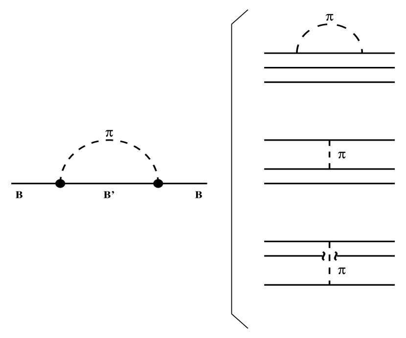
Figure 1: Self-energy model includes both loop effects and one-boson-exchange effects in a self-consistent calculation

It is important to note that the model used in this work not only self-consistently incorporates the effects on the properties of the quarks of self-energy loops, but also the effects of one-boson-exchange mechanism on baryon properties, since the created anti-quark can merge with any quark from the initial and final baryon to produce the intermediate meson. This point is illustrated in Figure 1. Calculations which treat only short distance interactions between quarks from the high momentum transfer limit of the last two diagrams on the right hand side of Figure 1 can be expected to neglect important effects from the self-consistent evaluation of quark self energies and exchange effects due to all mesons. They also do not properly take into account the two-hadron nature of the intermediate state at low momentum scales.

As mentioned before, and as it should also be apparent from the results of this work, conclusions made in prior works about spin-orbit forces in negative-parity excited baryon states were premature. Any calculation not including a complete set of spin-flavor symmetry related baryon-meson intermediate states, and excited baryon states up to at least the $N=3$ band, cannot claim to have complete results.

1 Outlook

After extensive work on this project there still remain many unanswered questions and unaddressed concerns. One important asset of the computational tools assembled for this project is their ability to be extended to larger sets of initial and intermediate hadrons given sufficient time and computing resources. Below, a few of the projects lined up behind this one are touched upon.

Since the framework is now in place, the next step is extension to the strange sector. The ground state $\Lambda$ and $\Sigma$ baryons as well as some of the experimentally better known $L=1$ negative-parity band $\Lambda$ and $\Sigma$ states are already under study. Experimental data for several of these states has recently improved, but agreement between the analyses of this experimental data and model predictions for resonance parameters is far from perfect. It will be interesting to find out how the baryon-meson loop induced self energies affect the splittings within this set of states.

As pointed out earlier, the inclusion of at least $N=4$ band baryon intermediate states will be required to bring about convergence of the intermediate state sum for $N=2$ band initial states. This should shed some light on the nature of some controversial and hard to model positive-parity states such as the Roper resonance. The computational tools used in this work are easily extended to such a calculation.

Mixing due to self energies must contribute to the splitting between baryons with same quantum numbers. Therefore studies of the mixing between the Nucleon and the Roper, the $N{\textstyle{1\over 2}}^{-}(1535)$ and $N{\textstyle{1\over 2}}^{-}(1650)$ states, and the $N{\textstyle{3\over 2}}^{-}(1520)$ and $N{\textstyle{3\over 2}}^{-}(1700)$ states will be required to further understand the impact of self energy loops on the splittings of these pairs of states.

The addition of spin-orbit interactions needs to be further explored. A preliminary study shows that the addition of spin-orbit interactions in the interactions leading to the wave functions used for the decay vertices can change the splitting between some states and even reverse the ordering of some of the states. More work is clearly needed in this area before conclusions can be drawn, as both the mixings due to self energies and spin-obit interactions strongly affect the masses of these states.

Even with these cautions, the present calculation goes far beyond anything previously available for the negative-parity non-strange baryons and shows, for the first time, results with a set of intermediate states large enough to achieve convergence. It also demonstrates for the first time the sensitivity of the self energies to the mixings caused by various components of the quark residual interactions.

Chapter 6 The Wave Functions

There are four components in each hadron wave function: color ($C$), flavor ($\phi$), spin ($\chi$), and spatial ($\psi$) wave functions.

Appendix 6.A Color

The meson color wave function is found by the rules of $SU(3)_{c}$ for direct products of quarks ($q$) and antiquarks ($\bar{q}$) carrying color charges or ${\bf 3}\otimes{\bf\bar{3}}={\bf 1}\oplus{\bf 8}$ and must be singlet to be an observable therefore it is

$$C^{M}=\sum_{i=1}^{3}\ \frac{1}{\sqrt{3}}\ q_{i}\ \bar{q}_{i}.$$ (1)

Similarly, the baryon color wave function is found by the same rules but for three quarks or ${\bf 3}\otimes{\bf 3}\otimes{\bf 3}={\bf 1}\oplus{\bf 8}\oplus{\bf 8^{\prime}}\oplus{\bf 10}$ to be the totally antisymmetric singlet combination

$$C_{A}^{B}=\sum_{i,j,k=1}^{3}\ \frac{1}{\sqrt{6}}\ \epsilon_{ijk}\ q_{1}^{i}\ q_{2}^{j}\ q_{3}^{k}.$$ (2)

Appendix 6.B Flavor

The flavor wave functions $\phi$ for the baryons and mesons included in this calculation are shown in Table 1. They are obtained from the irreducible representations of $SU(3)_{F}$ giving a flavor nonet each for the pseudoscalar mesons ($\pi,K,\bar{K},\eta,\eta^{\prime}$) and the vector mesons ($\rho,K^{*},\bar{K}^{*},\omega,\phi$).

For baryons, we follow the convention used in ref. [15] and adopt a generalized $uds$ basis that only symmetrizes the product $\phi\chi\psi$ in identical quarks. This removes the need for symmetrization between the $u$ and $d$ quarks in the spatial wave function making it manageable to work with states with up to $7\hbar\omega$ in the harmonic oscillator spectrum. Note that the baryon flavor wave functions are all either symmetric or antisymmetric under the interchange of quarks one and two.

Table 1: The baryon and meson flavor wave functions as a function of their isospin projection ($I_{z}$).

State	$+3/2$	$+1$	$1/2$	$0$	$-1/2$	$-1$	$-3/2$
$N$			$uud$		$ddu$
$\Delta$	$uuu$		$uud$		$ddu$		$ddd$
$\Lambda$				$\frac{1}{\sqrt{2}}(ud-du)s$
$\Sigma$		$uus$		$\frac{1}{\sqrt{2}}(ud+du)s$		$dds$
$\pi$		$-u\bar{d}$		$\frac{1}{\sqrt{2}}(u\bar{u}-d\bar{d})$		$+d\bar{u}$
$\rho$		$-u\bar{d}$		$\frac{1}{\sqrt{2}}(u\bar{u}-d\bar{d})$		$+d\bar{u}$
$K$			$-u\bar{s}$		$+s\bar{u}$
$K^{0}$			$-d\bar{s}$		$-s\bar{d}$
$\eta$				$\frac{1}{\sqrt{2}}\left[\frac{1}{\sqrt{2}}(u\bar{u}+d\bar{d})-s\bar{s}\right]$
$\eta^{\prime}$				$\frac{1}{\sqrt{2}}\left[\frac{1}{\sqrt{2}}(u\bar{u}+d\bar{d})+s\bar{s}\right]$
$\omega$				$\frac{1}{\sqrt{2}}(u\bar{u}+d\bar{d})$

Appendix 6.C Spin

The total spin of two spin-${\textstyle{1\over 2}}$ particles can be either zero or one giving us the pseudoscalar and vector mesons respectively.

The total spin of the three spin-${\textstyle{1\over 2}}$ particles can be either ${\textstyle{1\over 2}}$ or ${\textstyle{3\over 2}}$ so that as a complete set of spin wave functions $\chi$ we can choose

$$\chi^{S}_{{3\over 2}{3\over 2}} = |\uparrow\uparrow\uparrow\ \rangle\ \ ,\ \ {\rm{etc.}}$$ (3)

$$\chi^{M_{\rho}}_{{1\over 2}{1\over 2}} = {1\over\sqrt{2}}\left(\ |\uparrow\downarrow\uparrow\ \rangle-|\downarrow\uparrow\uparrow\ \rangle\ \right)\ \ ,\ \ {\rm{etc.}}$$ (4)

$$\chi^{M_{\lambda}}_{{1\over 2}{1\over 2}} = -{1\over\sqrt{6}}\left(\ |\uparrow\downarrow\uparrow\ \rangle+|\downarrow\uparrow\uparrow\ \rangle-2|\uparrow\uparrow\downarrow\ \rangle\ \right)\ \ ,\ \ {\rm{etc.}}$$ (5)

(We show only the top state of a JM multiplet; other wave functions follow the Condon-Shortley convention). Note that the baryon spin wave functions are also either symmetric or antisymmetric under interchange of the first two quarks.

Appendix 6.D Space

Finally, for the spatial wave functions $\Psi$ we take functions with definite total ${\bf L}={\bf l}_{\rho}+{\bf l}_{\lambda}$ made from a Clebsch-Gordan sum of harmonic oscillator wave functions in the two relative coordinates

$$\rho \equiv {1\over\sqrt{2}}({\bf r}_{1}-{\bf r}_{2})$$ (6)

and

$$\lambda \equiv {1\over\sqrt{6}}({\bf r}_{1}+{\bf r}_{2}-2{\bf r}_{3})$$ (7)

Figure 1: Relative coordinates $\rho$ and $\lambda$.

of the three body problem (see Figure 1). These are

$$\Psi_{{}_{LMn_{\rho}l_{\rho}n_{\lambda}l_{\lambda}}} = \alpha^{3}\sum_{m}C(l_{\rho}\,l_{\lambda}\,m\,M-m\,;\,L\,M){\cal{N}}_{n_{\rho}l_{\rho}}(\alpha\rho)^{l_{\rho}}e\,^{-{1\over 2}\alpha^{2}\rho^{2}}L_{n_{\rho}}^{l_{\rho}+{1\over 2}}(\alpha\rho)Y_{l_{\rho}m}(\Omega_{\rho})$$ (8)

$$\times{\cal{N}}_{n_{\lambda}l_{\lambda}}(\alpha\lambda)^{l_{\lambda}}e\,^{-{1\over 2}\alpha^{2}\lambda^{2}}L_{n_{\lambda}}^{l_{\lambda}+{1\over 2}}(\alpha\lambda)Y_{l_{\lambda}M-m}(\Omega_{\lambda}),$$

where the $L_{n}^{l+{1\over 2}}(x)$ are the associated Laguerre polynomials

$$L_{n}^{l+{1\over 2}}(x)=\sum_{m=0}^{n}(-1)^{m}{n+l+{1\over 2}\choose n-m}{x^{2m}\over m!}$$ (9)

(half-integral factorials are defined by the $\Gamma$ function), and the normalization coefficient ${\cal{N}}_{nl}$ is defined by

$${\cal{N}}_{nl}=\sqrt{2n!\over\Gamma(n+l+{3\over 2})}\ .$$ (10)

Putting all the elements together, the wave function is then expanded in a set of states of the form

$$|\alpha\ \rangle=C_{A}\Phi\sum_{M_{L}}C(L\,S\,M_{L}\,J-M_{L}\,;\,J\,M)\Psi_{{}_{LM_{L}n_{\rho}l_{\rho}n_{\lambda}l_{\lambda}}}\chi_{{}_{S\,M-M_{L}}}.$$ (11)

The entire wave function is now explicitly antisymmetric under the exchange of quarks one and two.

Chapter 7 Transition Amplitude

The final form of the transtition amplitude is

$$M_{A\to BC}={6\gamma\over 3\sqrt{3}}(-1)^{J_{a}+J_{b}+\ell_{a}+\ell_{b}-1}\sum_{J_{\rho},s_{a},s_{b}}{\hat{J}}\/_{\rho}^{2}\hat{s}_{a}{\hat{S}}\/_{a}{\hat{L}}\/_{a}\hat{s}_{b}{\hat{S}}\/_{b}{\hat{L}}\/_{b}$$

$$\left\{\matrix{S_{a}&L_{\rho}&s_{a}\cr\ell_{a}&J_{a}&L_{a}\cr}\right\}\left\{\matrix{L_{\rho}&S_{\rho}&J_{\rho}\cr{1\over 2}&s_{a}&S_{a}}\right\}\left\{\matrix{S_{b}&L_{\rho}&s_{b}\cr\ell_{b}&J_{b}&L_{b}\cr}\right\}\left\{\matrix{L_{\rho}&S_{\rho}&J_{\rho}\cr{1\over 2}&s_{b}&S_{b}}\right\}$$

$$(-1)^{\ell+\ell_{a}+J_{c}-L_{c}-S_{c}}{\cal F}(ABC){\cal R}(ABC)$$

$$\times\sum_{S_{bc}}(-1)^{s_{a}-S_{bc}}\left[\matrix{J_{\rho}&1/2&s_{b}\cr 1/2&1/2&S_{c}\cr s_{a}&1&S_{bc}}\right]\sum_{L_{bc}}(-1)^{L_{bc}}\left[\matrix{s_{b}&\ell_{b}&J_{b}\cr S_{c}&L_{c}&J_{c}\cr S_{bc}&L_{bc}&J_{bc}}\right]$$

$$\times\sum_{L}{\hat{L}}\/^{2}\left\{\matrix{s_{a}&\ell_{a}&J_{a}\cr L&S_{bc}&1}\right\}\left\{\matrix{S_{bc}&L_{bc}&J_{bc}\cr\ell&J_{a}&L}\right\}\varepsilon(\ell_{b},L_{c},L_{bc},\ell,\ell_{a},L,k_{0}).$$ (1)

Here

$${\bf J}_{a}={\bf L}_{a}+{\bf S}_{a}={\bf\ell}_{a}+{\bf s}_{a},$$ (2)

with

$${\bf L}_{a} = {\bf L}_{\lambda_{a}}+{\bf L}_{\rho_{a}}\equiv{\bf\ell}_{a}+{\bf L}_{\rho_{a}},$$

$${\bf S}_{a} = {\bf S}_{\rho_{a}}+{\bf 1/2},$$ (3)

and

$${\bf s}_{a} = {\bf J}_{\rho_{a}}+{\bf 1/2}={\bf L}_{\rho_{a}}+{\bf S}_{\rho_{a}}+{\bf 1/2},$$ (4)

with similar definitions for $B$. The first four $6-j$ symbols of Eq. (7) are necessary for transforming from the usual angular momentum basis for the baryons, given by Eq. (7), to the basis of Eq. (4), which is the more convenient one for evaluating the transition amplitude. $L$, $L_{bc}$ and $S_{bc}$ are internal summation variables, and ${\cal F}(ABC)$ is the flavor overlap for the decay.

The purely “spatial” part of the transition amplitude is

$$\varepsilon(\ell_{b},L_{c},L_{bc},\ell,\ell_{a},L,k_{0})={\cal J}(A)(-1)^{L_{bc}}{1\over 2}{\exp{(-F^{2}k_{0}^{2})}\over G^{\ell_{a}+\ell_{b}+L_{c}+4}}N_{a}N_{b}N_{c}$$

$$\times\sum_{\ell_{1},\ell_{2},\ell_{3},\ell_{4}}C^{\ell_{b}}_{\ell_{1}}C^{L_{c}}_{\ell_{2}}C^{1}_{\ell_{3}}C^{\ell_{a}}_{\ell_{4}}\left(x-\omega_{1}\right)^{\ell_{1}}\left(x-\omega_{2}\right)^{\ell_{2}}\left(x-1\right)^{\ell_{3}}x^{\ell_{4}}$$

$$\times\sum_{\ell_{12},\ell_{5},\ell_{6},\ell_{7},\ell_{8}}(-1)^{\ell_{12}+\ell_{6}}{\hat{\ell}_{5}\over\hat{L}}\left[\matrix{\ell_{1}&\ell_{1}^{\prime}&\ell_{b}\cr\ell_{2}&\ell_{2}^{\prime}&L_{c}\cr\ell_{12}&\ell_{6}&L_{bc}}\right]\left[\matrix{\ell_{3}&\ell_{3}^{\prime}&1\cr\ell_{4}&\ell_{4}^{\prime}&\ell_{a}\cr\ell_{7}&\ell_{8}&L}\right]$$

$$\times\left\{\matrix{\ell&\ell_{12}&\ell_{5}\cr\ell_{6}&L&L_{bc}}\right\}B^{\ell_{12}}_{\ell_{1}\ell_{2}}B^{\ell_{5}}_{\ell\ell_{12}}B^{\ell_{6}}_{\ell_{1}^{\prime}\ell_{2}^{\prime}}B^{\ell_{7}}_{\ell_{3}\ell_{4}}B^{\ell_{8}}_{\ell_{3}^{\prime}\ell_{4}^{\prime}}$$

$$\sum_{\lambda,\mu,\nu}D_{\lambda\mu\nu}(\omega_{1},\omega_{2},x)I_{\nu}(\ell_{5},\ell_{6},\ell_{7},\ell_{8};L)\left({\ell_{1}^{\prime}+\ell_{2}^{\prime}+\ell_{3}^{\prime}+\ell_{4}^{\prime}+2\mu+\nu+1\over 2}\right)!$$

$$\times k_{0}^{\ell_{1}+\ell_{2}+\ell_{3}+\ell_{4}+2\lambda+\nu}/G^{2\mu+\nu-\ell_{1}-\ell_{2}-\ell_{3}-\ell_{4}}.$$ (5)

In this expression, $N_{a}$ is a normalization coefficient that results from writing a single component of the wave function of $A$ as

$$\Psi_{LMn_{\rho}\ell_{\rho}n_{\lambda}\ell_{\lambda}}({\bf p}_{1},{\bf p}_{2},{\bf p}_{3})=\eta(AA^{\prime})^{3/2}\sum_{m}<\ell_{\rho}\ell_{\lambda}mM-m|LM>$$

$$\times{\cal N}_{n_{\rho}\ell_{\rho}}(A^{\prime}p_{\rho})^{\ell_{\rho}}e^{-{A^{\prime^{2}}p_{\rho}^{2}\over 2}}L_{n_{\rho}}^{\ell_{\rho}+1/2}(A^{\prime}p_{\rho})Y_{\ell_{\rho}m}({\bf\Omega}_{\rho})$$

$$\times{\cal N}_{n_{\lambda}\ell_{\lambda}}(Ap_{\lambda})^{\ell_{\lambda}}e^{-{A^{2}p_{\lambda}^{2}\over 2}}L_{n_{\lambda}}^{\ell_{\lambda}+1/2}(Ap_{\lambda})Y_{\ell_{\lambda}m}({\bf\Omega}_{\lambda}).$$ (6)

For proper exchange symmetry among the quarks, $A^{\prime}={2\over\sqrt{3}}A$, and

$${\bf p}_{\rho}={1\over 2}\left({\bf p}_{1}-{\bf p}_{2}\right),\,\,{\bf p}_{\lambda}={1\over 3}\left({\bf p}_{1}+{\bf p}_{2}-2{\bf p}_{3}\right).$$ (7)

$\eta$ is a phase factor that arises from calculating the Fourier transform of the configuration space wave functions, and has the value

$$\eta=(-i)^{2n_{\rho}+2n_{\lambda}+\ell_{\rho}+\ell_{\lambda}}.$$ (8)

With these definitions, $N_{a}=A^{\ell_{\lambda}+3/2}{\cal N}_{n_{\lambda}\ell_{\lambda}}$, with ${\cal N}_{n\ell}$ previously defined in 10, $L_{n}^{\ell+1/2}$ in 9, while the $Y_{\ell m}$ are the usual spherical harmonics.

${\cal J}$ is a Jacobian factor needed to convert from the basis used in evaluating the space factor $\varepsilon$ in Ref. [26], to the basis used in the evaluation of the wave functions used for explicit calculation of the decay amplitudes. The wave functions of Ref. [21] use

$${\bf p}_{\rho}^{\prime}={1\over\sqrt{2}}\left({\bf p}_{1}-{\bf p}_{2}\right),\,\,{\bf p}_{\lambda}^{\prime}={1\over\sqrt{6}}\left({\bf p}_{1}+{\bf p}_{2}-2{\bf p}_{3}\right),$$ (9)

so that both the Jacobian factor mentioned above, as well as a redefinition of the gaussian parameters of the wave functions, are required in order to use the wave functions of Ref. [21] with the above expression for the decay amplitude.

The factor ${\cal R}$ of Eq. (7) is obtained as the overlap of the wave functions in the $\rho$ coordinates in the initial and final baryon. Since in the model used here quarks $1$ and $2$ are spectators ($\ell_{\rho_{a}}=\ell_{\rho_{b}}$, $S_{\rho_{a}}=S_{\rho_{b}}$, $J_{\rho_{a}}=J_{\rho_{b}}$), and the basis is fully orthogonalized ($\alpha$ is the same in the initial and final baryons, so that $n_{\rho_{a}}=n_{\rho_{b}}$), this overlap is always unity. In addition, this means that the Jacobian discussed above is only necessary for the transformation in ${\bf p}_{\lambda}$.

The $\sum_{\lambda,\mu,\nu}D_{\lambda\mu\nu}(\omega_{1},\omega_{2},x)I_{\nu}(\ell_{5},\ell_{6},\ell_{7},\ell_{8};L)$ term arises from writing (here ${\bf q}_{a}\equiv{\bf p}_{\lambda_{a}}$, with a similar definition for the daughter baryon)

$$L_{n_{\lambda_{a}}}^{\ell_{a}}e^{-A^{2}q_{a}^{2}/2}L_{n_{\lambda_{b}}}^{\ell_{b}}e^{-B^{2}q_{b}^{2}/2}L_{n_{c}}^{L_{c}}e^{-C^{2}q_{c}^{2}/2}$$

$$\equiv\sum_{\lambda,\mu,\nu}D_{\lambda\mu\nu}(\omega_{1},\omega_{2},x)e^{-A^{2}q_{a}^{2}/2}e^{-B^{2}q_{b}^{2}/2}e^{-C^{2}q_{c}^{2}/2}.$$ (10)

When the substitutions ${\bf q}_{a}=x{\bf k}+{\bf q}$, ${\bf q}_{b}=(x-\omega_{1}){\bf k}+{\bf q}$, ${\bf q}_{c}=(x-\omega_{2}){\bf k}+{\bf q}$ are made, and the integrals over ${\bf k}$ and ${\bf q}$ are evaluated, the expression above results. The full form of the $D_{\lambda\mu\nu}$ does not provide additional information so it omitted.

In Eqs. (7) and (7),

$$\left[\matrix{a&b&c\cr d&e&f\cr g&h&i}\right]=\hat{c}\hat{f}\hat{g}\hat{h}\hat{i}\left\{\matrix{a&b&c\cr d&e&f\cr g&h&i}\right\}$$ (11)

where $\left\{\matrix{a&b&c\cr d&e&f\cr g&h&i}\right\}$ is the $9-j$ symbol, and ${\hat{J}}\/=\sqrt{2J+1}$.

In Eq. (7)

$$x = \left(B^{2}\omega_{1}+C^{2}\omega_{2}+f^{2}\right)\left(A^{2}+B^{2}+C^{2}+f^{2}\right)^{-1},$$

$$F^{2} = {1\over 2}\left[A^{2}x^{2}+B^{2}\left(x-\omega_{1}\right)^{2}+C^{2}\left(x-\omega_{2}\right)^{2}+f^{2}(x-1)^{2}\right],$$

$$G^{2} = {1\over 2}(A^{2}+B^{2}+C^{2}+f^{2}).$$ (12)

$\omega_{1}$ and $\omega_{2}$ are ratios of various linear combinations of quark masses. In general,

$$\omega_{1}={m_{1}+m_{2}\over m_{1}+m_{2}+m_{4}},\,\,\omega_{2}={m_{3}\over m_{3}+m_{4}},$$ (13)

where the subscripts refer to the quark labels shown in Figure 1. In addition,

$$C^{\ell}_{\ell_{1}} = \sqrt{{4\pi(2\ell+1)!\over(2\ell_{1}+1)![2(\ell-\ell_{1})+1]!}},$$

$$B^{\ell}_{\ell_{1}\ell_{2}} = {(-1)^{\ell}\over\sqrt{4\pi}}{\hat{\ell}}\/_{1}{\hat{\ell}}\/_{2}\left(\matrix{\ell_{1}&\ell_{2}&\ell\cr 0&0&0}\right),$$ (14)

and $\ell_{1}^{\prime}=L_{b}-\ell_{1}$, $\ell_{2}^{\prime}=L_{c}-\ell_{2}$, $\ell_{3}^{\prime}=1-\ell_{3}$, $\ell_{4}^{\prime}=L_{a}-\ell_{4}$ and the geometric factor $I_{\nu}$ is

$$I_{2p}(\ell_{5},\ell_{6},\ell_{7},\ell_{8};L)=(-1)^{L}(2p)!{\hat{\ell}}_{5}{\hat{\ell}}_{6}{\hat{\ell}}_{7}{\hat{\ell}}_{8}$$

$$\times\sum_{\lambda=0}^{p}{4^{\lambda}(4\lambda+1)(p+\lambda)!\over(2p+2\lambda+1)!(p-\lambda)!}\left(\matrix{2\lambda&\ell_{5}&\ell_{7}\cr 0&0&0}\right)\left(\matrix{2\lambda&\ell_{6}&\ell_{8}\cr 0&0&0}\right)\left\{\matrix{\ell_{5}&\ell_{6}&L\cr\ell_{8}&\ell_{7}&2\lambda}\right\},$$

$$I_{2p+1}(\ell_{5},\ell_{6},\ell_{7},\ell_{8};L)=2(-1)^{L+1}(2p+1)!{\hat{\ell}}_{5}{\hat{\ell}}_{6}{\hat{\ell}}_{7}{\hat{\ell}}_{8}$$

$$\times\sum_{\lambda=0}^{p}{4^{\lambda}(4\lambda+3)(p+\lambda+1)!\over(2p+2\lambda+3)!(p-\lambda)!}\left(\matrix{2\lambda+1&\ell_{5}&\ell_{7}\cr 0&0&0}\right)$$

$$\times\left(\matrix{2\lambda+1&\ell_{6}&\ell_{8}\cr 0&0&0}\right)\left\{\matrix{\ell_{5}&\ell_{6}&L\cr\ell_{8}&\ell_{7}&2\lambda+1}\right\}.$$ (15)

Chapter 8 Computational Methods

There are two main computational elements required to accomplish the calculation in this work. Recall the main equation of Chapter 1

$$Re[\Sigma_{B}(E)]=\sum_{B^{\prime}M}{\cal P}\int_{0}^{\infty}\frac{k^{2}dk{\cal M}_{BB^{\prime}M}^{\dagger}(k){\cal M}_{BB^{\prime}M}(k)}{E-\sqrt{M_{B^{\prime}}^{2}+k^{2}}-\sqrt{m_{M}^{2}+k^{2}}},$$ (1)

where ${\cal M}_{BB^{\prime}M}(k)$ is an expression for the momentum dependent vertex of the strong decay $B\rightarrow B^{\prime}M$, and ${\cal P}$ indicates that only the real part of the integral is evaluated by principal-part integration. How these components are computed is described in general terms in what follows, along with a sequence of how they are combined to produce the results presented in Chapter 4.

Appendix 8.A Strong Decay Vertices

The momentum dependence of the strong decay vertex can be obtained from the analytical form of the strong decay matrix element $\langle B^{\prime}M|T|B\rangle$, with $T$ representing the ${}^{3}P_{0}$ decay operator. The method used to evaluate these matrix elements is based on the work of Ref. [26] and Ref. [15], and several of the angular momentum techniques can be found in Ref. [28].

The symbolic manipulator Maple was used to compute all the components involved in calculating each decay matrix element for a large set of decays $B\rightarrow B^{\prime}M$. Subroutines were built to independently calculate each component so that it could be individually tested before being integrated into a higher level subroutine, and so that it could be totally portable. Basic procedures such as those to analytically calculate Clebsch-Gordan, $6-j$, or $9-j$ coefficients were implemented, along with generators of spherical harmonics and associated Laguerre polynomials. Then another series of algorithms were devised and coded to handle each component of Eq. 3 as defined in Appendix 7. The very large number of nested summations involved required careful and thorough testing as the trouble-shooting became more complex with each ‘layer’.

Due to the symmetry of the wave functions, in this ${}^{3}P_{0}$ model decays involving the first or second quark are considered separately from those involving the third quark of the decaying baryon. However, the two cases are related by a set of coefficients that, in effect, project a set of basis states onto another, or equivalently rotate a set of coordinates. The matrix elements can then be calculated in two different bases, and then combined after one set of results is transformed. These coefficients were adapted for this work from Moshinsky [29, 30, 31] brackets, coded, and then subsequently mass-produced with the results stored in analytical form. Once that was accomplished, it became possible to rapidly analytically compute matrix elements for decays from any initial baryon to any baryon-meson state, making this code a very versatile and powerful tool.

Since Maple is a powerful but slow program, and large parts of the analytical decay matrix elements are common for specific sets of quantum numbers, matrices of decay matrix elements were created between sets of hadron quantum numbers based on the expansion of the baryon wave functions. For example, matrices were built for decays from $J^{P}={\textstyle{3\over 2}}^{+}$ baryons (e.g. the $\Delta$ baryon) to $J^{P}={\textstyle{1\over 2}}^{+}$ baryons (e.g. the nucleon) and a pseudo-scalar meson (e.g. the pion). Since the baryon wave functions used in this project are expanded to the $N=6$ level (for positive-parity states and $N=7$ for negative-parity states) and thus have an average of about 100 components, for this example one matrix is 78 x 50, the other 152 x 100, with each element corresponding to a strong decay between a pair of basis substates. The process is repeated for decays involving vector mesons (e.g. the rho). Given the number of intermediate baryon-meson states included in this work, it is an understatement to say that this was a computer-intensive endeavor. It took several months to complete, using many nodes on the FSU Computer Cluster. Matrices were finally tested by using them to reproduce a large variety of published decay amplitudes [15, 22, 23].

The reward for this extensive calculation is the versatility of the code. Not only can it be used in the type of project described in this dissertation but, as mentioned above, it can also be applied to obtain any strong decay amplitude within the limits of the ${}^{3}P_{0}$ model. Since the decay matrix elements are stored in analytical form, changes in the value of any parameter can easily be handled without having to recalculate anything, and since wave function expansion coefficients are independent of the decay matrix elements, they can also be changed without affecting this part of the code.

Appendix 8.B Numerical Integration

Since the integrand of Eq. 1 can become extremely complex, it is not practical, and often not possible, to try to do the integration analytically, so numerical integration schemes were therefore used. Since both real (the initial baryon’s energy is above the threshold for production of the intermediate baryon-meson pair) and virtual (below threshold) decays are encountered, two different routines were used. In the case of virtual decays the integrand is always real, so a Gauss-Laguerre quadrature routine was used to perform the integration. Above threshold decays imply the presence of a pole, therefore a combination of Gauss-Laguerre and Gauss-Legendre type quadratures were used to integrate symmetrically around the pole and evaluate the principal part of Eq. 1.

The integration routines were developed using the C programming language, and used modified versions of pre-coded numerical algorithms from Ref. [32].

Appendix 8.C Overall Scheme

The numerator of Eq. 1 is obtained via a Maple routine which performs the matrix algebra required to combine the matrices of decay matrix elements with the appropriate vectors of wave function expansion coefficients. The result is an analytical expression as a function $k$ which is then translated into C code by Maple. The result is then used by the integration routine.

During the matrix algebra part of the calculation, it was found that the amount of time required to process analytical matrices ranging in size from 150 MB (for decays involving pseudo-scalar mesons) to well over 650 MB (for decays involving vector mesons) could limit the number of intermediate baryon-meson states included. Since a crucial ingredient of the calculation is the large extent of the sum over intermediate states, an additional routine was implemented to ‘preprocess’ the matrices by assigning numerical values to the parameters that were common to a set of initial states (based on a given set of baryon wave functions), which were then stored in new matrices for use when needed. This extra step, added at the cost of a few days of processing for each new set of matrices, cut the final matrix algebra time by a factor of roughly 60%, making it possible to compare multiple sets of results within a reasonable time frame.

For each initial baryon and each baryon-meson combination in the sum over intermediate states ($\sum_{B^{\prime}M}$), the associated integral is evaluated for 200 different values of $E$ over the energy range being considered. These values are then tabulated and then used to produce graphs such as those presented in Chapter 4.

Throughout this process, liberal use is made of scripts (both in Maple and Unix) to handle the large number of intermediate states and automate the process as much as possible.

References

- [1] F.J. Yndurain, The Theory of Quark and Gluon Interactions, Springer-Verlag, 1999.
- [2] W. Greiner, S. Schramm, and E. Stein, Quantum Chromodynamics, Springer-Verlag, 2000.
- [3] F. Gross, Relativistic Quantum Mechanics and Field Theory, John Wiley & Sons, 1999.
- [4] K. G. Wilson, Phys. Rev. D10, 2445 (1974).
- [5] M. Creutz, Quarks, gluons and lattices, Cambridge University Press, 1983.
- [6] P. Zenczykowski, Ann. Phys. (NY) 169 453 (1986); N. A. Tornqvist and P. Zenczykowski, Z. Phys. C30, 83 (1986); Phys. Rev. D29, 2139 (1984).
- [7] A. De Rujula, H. Georgi and S.L. Glashow, Phys. Rev. D12, 147 (1975).
- [8] W. Blask, M.G. Huber, and B. Metsch, Z. Phys. A326, 413 (1987).
- [9] M. Brack and R. K. Bhaduri, Phys. Rev. D35, 3541 (1987).
- [10] P. Geiger and N. Isgur, Phys. Rev. D44, 799 (1991).
- [11] K. G. Horacsek, Y. Iwamura and Y. Nogami, Phys. Rev. D32, 3001 (1985).
- [12] B. Silvestre-Brac and C. Gignoux, Phys. Rev. D43, 3699 (1991).
- [13] Y. Fujiwara, Prog. Th. Phys. 89, 455 (1993).
- [14] E.S. Ackleh, T. Barnes and E. Swanson, Phys. Rev. D54, 6811 (1996).
- [15] S. Capstick and W. Roberts, Phys. Rev. D47, 1994 (1993).
- [16] N. Isgur and G. Karl, Phys. Lett. 72B, 109 (1977).
- [17] N. Isgur and G. Karl, Phys. Lett. 74B, 353 (1978).
- [18] N. Isgur and G. Karl, Phys. Rev. D18, 4187 (1978).
- [19] N. Isgur and G. Karl, Phys. Rev. D20, 1191 (1979).
- [20] S. Godfrey and N. Isgur, Phys. Rev. D32, 189 (1985).
- [21] S. Capstick and N. Isgur, Phys. Rev. D34, 2809 (1986).
- [22] S. Capstick and W. Roberts, Phys. Rev. D49, 4570 (1994).
- [23] S. Capstick and W. Roberts, Phys. Rev. D58, 074011 (1998).
- [24] S. Capstick and W. Roberts, Prog. Part. Nucl. Phys. 45, S241 (2000).
- [25] A. Le Yaouanc, L. Oliver, O. Pène and J. C. Raynal, Hadron Transitions In The Quark Model, Gordon and Breach, 1988.
- [26] W. Roberts and B. Silvestre-Brac, Few Body Syst. 11, 171 (1992).
- [27] A.J. Buchmann, E. Hernández and A. Faessler, Phys. Rev. C55, 448 (1997).
- [28] D.A. Varshalovich, A.N. Moskalev, V.K. Khersonskii,Quantum Theory of Angular Momentum, World Scientific Publishing, 1988.
- [29] M. Moshinsky, Nucl. Phys. 13, 104 (1959).
- [30] T.A. Brody and M. Moshinsky, Tables of Transformation Brackets for Nuclear Shell-Model Calculations, Gordon and Breach, 1967.
- [31] M. Moshinsky, The Harmonic Oscillator in Modern Physics: From Atoms to Quarks, Gordon and Breach, 1969.
- [32] W.H. Press et al., Numerical Recipes in C : the art of scientific programming, Cambridge University Press, 1992.
- [33] P. Geiger and N. Isgur, Phys. Rev. D41, 1595 (1990).