Compatibility of localized wave packets and unrestricted single particle dynamics for cluster formation in nuclear collisions

Abstract

Antisymmetrized molecular dynamics with quantum branching is generalized so as to allow finite time duration of the unrestricted coherent mean field propagation which is followed by the decoherence into wave packets. In this new model, the wave packet shrinking by the mean field propagation is respected as well as the diffusion, so that it predicts a one-body dynamics similar to that in mean field models. The shrinking effect is expected to change the diffusion property of nucleons in nuclear matter and the global one-body dynamics. The central ${}^{129}\mathrm{Xe}+\mathrm{Sn}$ collisions at 50 MeV/nucleon are calculated by the models with and without shrinking, and it is shown that the inclusion of the wave packet shrinking has a large effect on the multifragmentation in a big expanding system with a moderate expansion velocity.

I Introduction

In order to describe heavy ion reactions as the dynamics of many-nucleon systems, two different kinds of microscopic approaches have been proposed and applied. One is the molecular dynamics models AICHELIN ; MARUb ; ONOab ; FELDMEIER and the other is the mean field (TDHF-like) models BERTSCH ; CASSING . An advantage of the mean field models is that they do not put any restriction on the one-body motion, while their disadvantage is that they cannot properly describe the cluster formation because of the lack of many-body cluster correlations. On the other hand, usual molecular dynamics models assume a fixed Gaussian shape for single particle wave functions. This is an efficient way to describe the cluster correlation even by using a simple product wave function with or without antisymmetrization. However, in another sense, the use of localized wave packets can be a regression because the one-body dynamics is not as precisely described as in mean field models.

An unified understanding is desired on the question whether the single particle wave functions should be unrestricted or localized. Unless we can solve the dynamics keeping the full order of the many-body correlations, it is essential for a reasonable model to introduce the fluctuations which bring the system into many quantum branches each of which corresponds to one of the reaction channels or the configurations of clusterization. In mean field models, it has been proposed to introduce fluctuations in the one-body distribution function AYIK ; RANDRUP , though it should be a difficult problem to determine the correlations among an infinite number of the degrees of freedom of fluctuations. In this viewpoint, the philosophy of molecular dynamics is to introduce a special kind of fluctuation by stochastically localizing the single particle wave functions, which is essential for the cluster production. The mean field equation should be interpreted as giving the short-time evolution of the one-body distribution averaged over the stochastic branches. Based on this idea, the antisymmetrized molecular dynamics (AMD) has been extended in Refs. ONOh ; ONOi by incorporating the wave packet diffusion effect in the mean field as a source of the fluctuation to the wave packet centroid which causes the quantum branching on the many-body level. Thus the single particle wave functions are localized in each branch, which makes cluster formation possible, while the single particle motion is not restricted for the averaged value over the branches. The stochastic treatment of the dynamics of the wave packet width is the essential point of our approach. There is another approach FELDMEIER ; KIDERLEN ; CHOMAZ ; MARU-EQMD which treats the width parameters as time-dependent variables in molecular dynamics, though it has turned out that the deterministic dynamics of the width variables cannot explain the evolution of the density fluctuation and the multiple cluster formation KIDERLEN ; CHOMAZ . Ohnishi and Randrup OHNISHI-RANDRUPb ; OHNISHI-RANDRUPc have introduced quantum fluctuation into wave packet molecular dynamics based on their statistical consideration and have shown its importance in cluster formation. However the dynamical origin of the their fluctuation has not been made clear.

An unsatisfactory point of the improvement in Refs. ONOh ; ONOi was that the stochastic fluctuation to the wave packet centroids can diffuse the distribution but cannot shrink the distribution. Note that a wave packet in the mean field normally diffuses in three directions in phase space and shrinks in the other three directions. Because of this difficulty, for example, the improved AMD could not be directly applied to an isolated nucleon, and therefore the diffusion was switched off for isolated nucleons, which introduces an ambiguity to the model. To solve this kind of problems, we absolutely need a consistent understanding of both the mean field description and the molecular dynamics description.

The first purpose of the present work is to construct a general framework which contains both molecular dynamics models and mean field models as specific cases. In this framework, the time evolution of a many-body system is given by the coherent mean field propagation and the decoherence of single particle states into wave packets. It will have two physically essential ingredients, $\tau$ and $\tau_{\text{mf}}$, which define when “decoherence” and “mean field branching” take place, respectively. The choice $(\tau,\tau_{\text{mf}})=(\infty,\infty)$ corresponds to a mean field model, while the choice $(\tau,\tau_{\text{mf}})=(0,0)$ corresponds to the version of AMD of Refs. ONOh ; ONOi (called AMD/D in this paper). Based on this general framework, we introduce a new model AMD/DS as the case of $(\tau,\tau_{\text{mf}})=(\text{large},0)$, with which we can respect not only the diffusion but also the shrinking of the phase space distribution predicted by the coherent mean field propagation.

The second purpose of the present work is to demonstrate the effect of the wave packet shrinking. The difference between AMD/D and AMD/DS is expected to result in the different diffusion properties of nucleons in nuclear matter and the different global one-body dynamics. We perform the AMD/D and AMD/DS calculations for the central ${}^{129}\mathrm{Xe}+\mathrm{Sn}$ collisions at 50 MeV/nucleon and compare the results. The velocity of the expansion strongly depends on the model. The different expansion velocity results in the different cluster size distribution. It is shown, by comparison with INDRA experimental data, that AMD/D had problems of the overestimation of $Z=4,5,6$ clusters and the underestimation of $Z\gtrsim 15$ clusters and these problems are solved by AMD/DS.

This paper is organized as follows. In Sec. II, the formulation is presented. The physical principle of the general framework is given in II.1, and then the concrete formulae are given in II.2 which includes all the details. In II.3, we introduce specific models such as AMD/D and AMD/DS, and give simple examples to show how our formulation works for AMD/D and AMD/DS. In Sec. III, the results of the calculations with AMD/D and AMD/DS are compared to each other and to the INDRA data for central ${}^{129}\mathrm{Xe}+\mathrm{Sn}$ collisions at 50 MeV/nucleon, so as to demonstrate the important effect of the wave packet shrinking in AMD/DS in multifragmentation. Section IV is devoted to a summary.

II Mean field propagation followed by decoherence

II.1 Principle

First we give a general framework which includes both mean field models and molecular dynamics models as limiting cases of model parameters. Originally we have reached this framework in the course of an extension of AMD by the incorporation of good points of mean field models. However, the framework is given here from a more general point of view as an approximation of quantum many-body dynamics.

In what follows, the two-nucleon collision effect is not shown explicitly for the brevity of presentation, but it is always considered in all the practical calculations as a stochastic process ONOab ; ONOd .

In this model, we will use (without specifying yet how to use it) the AMD wave function which is a Slater determinant of Gaussian wave packets ONOab ,

$$\langle\mathbf{r}_{1}\ldots\mathbf{r}_{A}|\Phi(Z)\rangle=\det_{ij}\Bigl{[}\exp\Bigl{\{}-\nu\Bigl{(}\mathbf{r}_{j}-\frac{\mathbf{Z}_{i}}{\sqrt{\nu}}\Bigr{)}^{2}\Bigr{\}}\chi_{\alpha_{i}}(j)\Bigr{]}.$$ (1)

The complex variables $Z\equiv\{\mathbf{Z}_{i};\ i=1,\ldots,A\}$ represent the centroids of the wave packets. We take the width parameter $\nu=0.16$ $\mathrm{fm}^{-2}$ and the spin isospin states $\chi_{\alpha_{i}}=p\uparrow$, $p\downarrow$, $n\uparrow$, or $n\downarrow$. Because of the antisymmetrization, the variables $Z$ do not necessarily have a direct physical meaning as nucleon positions and momenta. The AMD wave function $|\Phi(Z)\rangle$ contains many quantum features in it and has been applied to the study of nuclear structure problems with some extensions such as the parity and angular momentum projections ENYO .

The time-dependent many body wave function $|\Psi(t)\rangle$ describing a complicated nuclear collision is, in an intermediate or final state, a superposition of a huge number of channels each of which corresponds to a different clusterization configuration. We do not try to directly treat such a complicated many-body state $|\Psi(t)\rangle$ nor we do not approximate $|\Psi(t)\rangle$ by a single AMD wave function $|\Phi(Z)\rangle$. We rather approximate the many-body density matrix $|\Psi(t)\rangle\langle\Psi(t)|$ by an ensemble of many AMD wave functions,

$$|\Psi(t)\rangle\langle\Psi(t)|\approx\int\frac{|\Phi(Z)\rangle\langle\Phi(Z)|}{\langle\Phi(Z)|\Phi(Z)\rangle}w(Z,t)dZ.$$ (2)

A pure many-body state is approximated by a mixed state. This approximation itself will not be a serious drawback practically because the nuclear collision dynamics is so complicated that one cannot observe full many-body correlations to distinguish a pure state from a mixed state. The benefit of this approximation is that the right hand side of Eq. (2) still contains nontrivial many-body correlations required in multiple cluster formation, even though an ensemble of AMD wave functions is sufficiently simple to be tractable numerically. We should, of course, define a reasonable time evolution of the weight $w(Z,t)$ or, alternatively, stochastic trajectories of the variables $Z(t)$.

What is the physical idea when we use AMD wave functions $|\Phi(Z)\rangle$ in Eq. (2)? When multiple cluster formation takes place, $|\Psi(t)\rangle$ is composed of a huge number of branches. The decomposition into branches should be done so that, in each branch, the one-body distribution of each nucleon is localized in one of the clusters. Namely, a nucleon should not belong to many clusters at the same time, to avoid non-integer mass numbers of clusters. [The width of wave packets $\nu$ has been chosen in such a way.] In turn, if nucleons are localized in each branch, the clusters are naturally bound due to the mean field among localized nucleons. This idea exists behind the molecular dynamics models which restrict each single particle wave function in each branch to a wave packet.

The time evolution in our model is determined by two factors, the mean field propagation and the decomposition into branches. At a time $t_{0}$, let us take one of the branches $|\Phi(Z)\rangle\langle\Phi(Z)|$ from Eq. (2). This is justified because the time evolution of a branch is independent of the others due to linear quantum mechanics. We consider the mean field propagation from $t_{0}$ to $t_{0}+\tau$,

$$|\Phi(Z)\rangle\langle\Phi(Z)|\rightarrow|\Psi(\tau,Z)\rangle\langle\Psi(\tau,Z)|,$$ (3)

where $|\Psi(\tau,Z)\rangle$ is the solution of the mean field equation

$$i\hbar\frac{d}{dt}|\Psi(t,Z)\rangle=H^{\mathrm{HF}}(t)|\Psi(t,Z)\rangle$$ (4)

with the initial condition $|\Psi(0,Z)\rangle=|\Phi(Z)\rangle$. The mean field Hamiltonian has a form

$$H^{\mathrm{HF}}(t)=\sum_{i=1}^{A}h_{i}(t)=\sum_{i=1}^{A}\biggr{(}\frac{\mathbf{p}_{i}^{2}}{2M}+U(\mathbf{r}_{i},\mathbf{p}_{i};\hat{\rho}(t))\biggr{)},$$ (5)

where the potential $U$ depends on a one-body density matrix $\hat{\rho}(t)$. For the moment, we may assume that $\hat{\rho}(t)$ is the one-body density matrix for the state $|\Psi(t,Z)\rangle$. We wish to emphasize that the single particle wave functions are not restricted to Gaussian packets in the mean field propagation and therefore $|\Psi(\tau,Z)\rangle$ is a general Slater determinant. Next, at the time $t_{0}+\tau$, the propagated state $|\Psi(\tau,Z)\rangle\langle\Psi(\tau,Z)|$ is decomposed into AMD wave functions as

$$\frac{|\Psi(\tau,Z)\rangle\langle\Psi(\tau,Z)|}{\langle\Phi(Z)|\Phi(Z)\rangle}\approx\int\frac{|\Phi(z)\rangle\langle\Phi(z)|}{\langle\Phi(z)|\Phi(z)\rangle}w(z,\tau;Z)dz,$$ (6)

with a suitable weight $w(z,\tau;Z)$. A reasonable principle to determine $w(z,\tau;Z)$ would be first to choose a set of important (one-body) operators $\{\hat{O}_{\alpha}\}$ and then to require that both sides of Eq. (6) give the same expectation values for all $\{\hat{O}_{\alpha}\}$,

$$\int\frac{\langle\Phi(z)|\hat{O}_{\alpha}|\Phi(z)\rangle}{\langle\Phi(z)|\Phi(z)\rangle}w(z,\tau;Z)dz=\frac{\langle\Psi(\tau,Z)|\hat{O}_{\alpha}|\Psi(\tau,Z)\rangle}{\langle\Phi(Z)|\Phi(Z)\rangle}.$$ (7)

However, this prescription will not always work well because it is incompatible to the necessary condition $w(z,\tau;Z)\geq 0$. A practical choice of $\{\hat{O}_{\alpha}\}$ will be given bellow. In this way, in principle, Eq. (3) and Eq. (6) determine the time evolution from $t_{0}$ to $t_{0}+\tau$. The next time evolution after $t_{0}+\tau$ is obtained successively by applying the same model to each term of the right hand side of Eq. (6).

What is the physical meaning of $\tau$? Is Eq. (6) just a numerical approximation of a mean field model or does it have any physical meaning? Once one believes that the mean field propagation were always perfect, then the choice of a finite $\tau$ would be unphysical. But the mean field propagation is not perfect at least in that it unphysically keeps the idempotency $\hat{\rho}^{2}=\hat{\rho}$ of the one-body density matrix. In many-body systems, even though the idempotency is satisfied at a time, it is not the case at a later time due to many-body correlations. The reduced one-body density matrix will be an ensemble of idempotent density matrices. If we ignore the antisymmetrization for the simplicity of the discussion here, the one-body density matrix of a nucleon will be given like

$$\hat{\rho}=w^{\prime}|\varphi^{\prime}\rangle\langle\varphi^{\prime}|+w^{\prime\prime}|\varphi^{\prime\prime}\rangle\langle\varphi^{\prime\prime}|+\cdots,$$ (8)

in which different components $|\varphi^{\prime}\rangle$, $|\varphi^{\prime\prime}\rangle$,… do not interfere in a simple way. The many-body state for this situation will be like

$$|\Psi\rangle=c^{\prime}|\varphi^{\prime}\rangle\otimes|\tilde{\Psi}^{\prime}\rangle+c^{\prime\prime}|\varphi^{\prime\prime}\rangle\otimes|\tilde{\Psi}^{\prime\prime}\rangle+\cdots,$$ (9)

where the states of the rest of the system $|\tilde{\Psi}^{\prime}\rangle$, $|\tilde{\Psi}^{\prime\prime}\rangle$, … are orthogonal to one another, to have Eq. (8). In our model, the coherent mean field propagation ($|\Psi\rangle=|\varphi\rangle\otimes|\tilde{\Psi}\rangle$) is assumed to be valid in the time duration from $t_{0}$ to $t_{0}+\tau$, and “decoherence” is assumed to physically take place into Gaussian packets at $t_{0}+\tau$ as in Eq. (8) and Eq. (9). [“Decoherence” is a general concept of quantum mechanics in open systems ZUREK . It means not only that Eq. (8) is satisfied at a specific time but also that different branches do not interfere at any later time.] In this way, the parameter $\tau$ has a deep physical meaning as the coherence time. We do not try to determine $\tau$ a priori in the present paper, but we assume that decoherence is a physical process as should be the case at least in multiple cluster formation. It should be noted that the physical state changes by decoherence, and therefore Eq. (7) should not be required for all the operators $\{\hat{O}_{\alpha}\}$. We should require Eq. (7) for those operators $\{\hat{O}_{\alpha}\}$ which we can believe to remain after physical decoherence.

Closely related to the decoherence of a nucleon, we should decide how this nucleon interacts with the rest of the system, namely, how this nucleon contributes to the mean field potential $U$. Once decoherence takes place at $t_{0}+\tau$ so that different branches in Eq. (9) do not interfere any longer, then the mean field should be calculated in each branch, independently of the other branches, by using the corresponding wave packet (one of $|\varphi^{\prime}\rangle$, $|\varphi^{\prime\prime}\rangle$, …). We will call this change of the mean field “mean field branching”. The decomposition of the many body state in Eq. (6) is consistent to the mean field branching at $t_{0}+\tau$. Nevertheless, we may think of the other possibility that the time scale of mean field branching, denoted by $\tau_{\text{mf}}$, is shorter than $\tau$. The choice $\tau_{\text{mf}}<\tau$ can be reasonable in such a physical situation that, even before decoherence, the mean field approximation is applicable not to $|\Psi\rangle$ of Eq. (9) but to each of the “pre-branches” in the right hand side of Eq. (9) even when the pre-branches have not been decohered yet (i.e., $|\tilde{\Psi}^{\prime}\rangle$, $|\tilde{\Psi}^{\prime\prime}\rangle$, … are not orthogonal). This situation is possible because the true time evolution is linear while the mean field approximation is nonlinear. Therefore we regard $\tau_{\text{mf}}$ as a physical ingredient of the model which is not necessarily equal to $\tau$.

The physical origin of decoherence we have in mind here is the full oder of many-body correlations beyond the two-body correlation, which is especially important in multiple cluster formation. The choice of wave packets as decohered states is done for this purpose. Of course, the two-body collision effect destroys the idempotency of the one-body density matrix, but this effect is already taken into account by a more explicit way of the stochastic two-nucleon collision process ONOab ; ONOd in all the realistic calculations.

II.2 Formulation

Now we start to give concrete formulae for the calculation of the time evolution governed by the mean field propagation followed by the decoherence into stochastic branches. The explanation will be given by five steps.

Impatient readers may be able to skip this part first moving to Sec. II.3, and later come back here if necessary.

II.2.1 Physical coordinate approximation

We adopt the “physical coordinate approximation” for an AMD wave function,

$$\frac{|\Phi(Z)\rangle\langle\Phi(Z)|}{\langle\Phi(Z)|\Phi(Z)\rangle}\approx\bigotimes_{k=1}^{A}\frac{|\varphi(\mathbf{W}_{k})\chi_{\alpha_{k}}\rangle\langle\varphi(\mathbf{W}_{k})\chi_{\alpha_{k}}|}{\langle\varphi(\mathbf{W}_{k})\chi_{\alpha_{k}}|\varphi(\mathbf{W}_{k})\chi_{\alpha_{k}}\rangle}$$ (10)

where the spatial wave function of each nucleon $k$ is given by a Gaussian packet

$$\langle\mathbf{r}|\varphi(\mathbf{W}_{k})\rangle=\exp\Bigl{\{}-\nu\Bigl{(}\mathbf{r}-\frac{\mathbf{W}_{k}}{\sqrt{\nu}}\Bigr{)}^{2}\Bigr{\}}.$$ (11)

The centroids are the physical coordinates $W=\{\mathbf{W}_{k}\}$ defined in Ref. ONOab by

$$\mathbf{W}_{k}=\sqrt{\nu}\,\mathbf{R}_{k}+\frac{i}{2\hbar\sqrt{\nu}}\mathbf{P}_{k}=\sum_{j=1}^{A}\Bigl{(}\sqrt{Q}\Bigr{)}_{kj}\mathbf{Z}_{j},$$ (12)

$$Q_{kj}=B_{kj}B^{-1}_{jk},\qquad B_{kj}=e^{\mathbf{Z}_{k}^{*}\cdot\mathbf{Z}_{j}}\delta_{\alpha_{k}\alpha_{j}}.$$ (13)

In the phase space representation, the Wigner function for the nucleon $k$ is given by a Gaussian packet

$$g(x;X_{k})=8\exp\biggr{[}-2\sum_{a=1}^{6}(x_{a}-X_{ka})^{2}\biggr{]},$$ (14)

where we have introduced the 6-dimensional phase space coordinates

$$x=\{x_{a};\ a=1,\ldots,6\}=\biggl{\{}\sqrt{\nu}\,\mathbf{r},\ \frac{\mathbf{P}_{k}}{2\hbar\sqrt{\nu}}\biggr{\}},$$ (15)

$$X_{k}=\{X_{ka};\ a=1,\ldots,6\}=\biggl{\{}\sqrt{\nu}\,\mathbf{R}_{k},\ \frac{\mathbf{P}_{k}}{2\hbar\sqrt{\nu}}\biggr{\}}.$$ (16)

We wish to emphasize that much of the fermionic feature remains even though we adopt the physical coordinate approximation [Eq. (10)]. This is because the value of $W$ carries the fermionic information. For example, in the $6A$-dimensional space of $W$, there exists Pauli forbidden region where $W$ cannot take value for any choice of the original coordinate $Z$ ONOab . Nevertheless, it depends on the purpose whether this approximation gives a good result. For example, it gives only a poor approximation for the evaluation of the Hamiltonian and the mean field potential. For the calculation of such quantities, we use the exact antisymmetrized wave function $|\Phi(Z)\rangle$ or use a better approximation scheme ONOi .

II.2.2 Mean field propagation

The mean field propagation [Eq. (3)] from $t_{0}$ to $t_{0}+\tau$ is calculated based on the Vlasov equation with the “Gaussian-Gaussian approximation” whose exact meaning is given bellow.

We require that the Wigner function $\bar{f}_{k}(x,t)$ of the nucleon $k$ should satisfy the Vlasov equation

$$\frac{\delta\bar{f}_{k}}{\delta t}=-\frac{\partial h}{\partial\mathbf{p}}\cdot\frac{\partial\bar{f}_{k}}{\partial\mathbf{r}}+\frac{\partial h}{\partial\mathbf{r}}\cdot\frac{\partial\bar{f}_{k}}{\partial\mathbf{p}},$$ (17)

at least approximately, for the time interval from $t_{0}$ to $t_{0}+\tau$, with the initial condition $\bar{f}_{k}(x,0)=g(x;X_{k})$. A special notation of the time derivative ($\delta/\delta t$) is adopted for the mean field propagation in order to avoid a future possible confusion. Of course, it would be an easy numerical task to solve Eq. (17) directly. However, in order to make the later decoherence process as simple as possible, we take another method by writing the Wigner function as the mean of the stochastic virtual phase space distributions of deformed Gaussian shape,

$$\bar{f}_{k}(x,t) =\overline{g(x;X_{k}(t),S_{k}(t))}$$

$$=\int g(x;X,S_{k}(t))w_{k}(X,t)\frac{d^{6}X}{\pi^{3}},$$ (18)

with

$$g(x;X,S)=\frac{1}{8\sqrt{\det{S}}}\exp\biggr{[}-\frac{1}{2}\sum_{ab=1}^{6}S^{-1}_{ab}(x_{a}-X_{a})(x_{b}-X_{b})\biggr{]}.$$ (19)

Thus we have the virtually stochastic variables $X_{ka}(t)$ and $S_{kab}(t)$ which represent the centroid and the shape, respectively, of the virtually stochastic distribution $g(x,X_{k}(t),S_{k}(t))$. The initial condition for them can be given by $X_{ka}(0)=X_{ka}$ and $S_{kab}(0)=\frac{1}{4}\delta_{ab}$ at the initial time $t_{0}$ [Eq. (14)]. The stochasticity of $S_{kab}(t)$ is not shown explicitly in Eq. (18) because we will see later that its stochasticity is weak.

We shall now determine the virtually stochastic time evolution of $X_{ka}(t)$ and $S_{kab}(t)$. It is first noticed that the Vlasov equation can be applied to each component of Eq. (18) as long as Eq. (17) is linear in $\bar{f}_{k}$. The time evolution of $g_{k}(x,X_{k}(t),S_{k}(t))$ by the Vlasov equation

$$\frac{\delta g}{\delta t}=-\frac{\partial h}{\partial\mathbf{p}}\cdot\frac{\partial g}{\partial\mathbf{r}}+\frac{\partial h}{\partial\mathbf{r}}\cdot\frac{\partial g}{\partial\mathbf{p}},$$ (20)

is characterized by the time evolution of the first and the second moments of the distribution

$$\frac{\delta}{\delta t}{X}_{ka}(t)=\frac{\delta}{\delta t}\int x_{a}g(x,t)\frac{d^{6}x}{\pi^{3}},$$ (21)

$$\frac{\delta}{\delta t}{S}_{kab}(t)=\frac{\delta}{\delta t}\int\Bigl{(}x_{a}-X_{ka}(t)\Bigr{)}\Bigl{(}x_{b}-X_{kb}(t)\Bigr{)}g(x,t)\frac{d^{6}x}{\pi^{3}},$$ (22)

in which $(\delta/\delta t)g(x,t)$ is given by Eq. (20). The shape of the distribution at $t+\Delta t$ is characterized by $S_{kab}(t)+(\delta/\delta t){S}_{kab}(t)\Delta t$. This symmetric matrix is diagonalized by an orthogonal matrix as

$$S_{kab}(t)+\frac{\delta}{\delta t}{S}_{kab}(t)\Delta t=\sum_{c}\lambda_{c}O_{ac}O_{bc}.$$ (23)

The distribution is generally diffusing in some directions and shrinking in the other directions in the phase space. We will extract the component that is diffusing beyond the original width of the wave packet [Eq. (14)] by

$$\Bigl{(}\frac{\delta}{\delta t}S_{kab}(s)\Bigr{)}_{+}=\lim_{\Delta t\rightarrow 0}\frac{1}{\Delta t}\sum_{c}\max\Bigl{(}0,\ \lambda_{c}-{\textstyle\frac{1}{4}}\Bigr{)}O_{ac}O_{bc},$$ (24)

which is now taken into account, not by changing the variable $S_{kab}(t)$, but by giving a virtual Gaussian fluctuation $\Delta X_{ka}(t)$ to the centroid $X_{ka}(t)$ satisfying

$$\overline{\Delta X_{ka}(t)}=0,$$ (25a)

$$\overline{\Delta X_{ka}(t)\Delta X_{kb}(t^{\prime})}=\Bigl{(}\frac{\delta}{\delta t}S_{kab}(t)\Bigr{)}_{+}\delta(t-t^{\prime}).$$ (25b)

The equation of motion for $X_{ka}(t)$ with virtual stochasticity may be written as

$$\frac{d}{dt}X_{ka}(t)=\frac{\delta}{\delta t}X_{ka}(t)+\Delta X_{ka}(t).$$ (26)

The equation of motion for $S_{kab}(t)$ is

$$\frac{d}{dt}S_{kab}(t)=\frac{\delta}{\delta t}{S}_{kab}(t)-\Bigl{(}\frac{\delta}{\delta t}{S}_{kab}(t)\Bigr{)}_{+},$$ (27)

which does not contain the diffusing component beyond the original width because its effect has been counted as the fluctuation to $X_{kab}(t)$.

We emphasize again that the stochasticity has been, at this stage, introduced only as a numerical method to solve the mean field propagation [Eq. (17)]. By taking the mean of the ensemble of stochastic distributions $g(x,X_{k}(t),S_{k}(t))$ [Eq. (18)], our solution will reproduce the deterministic solution of Eq. (17), up to the Gaussian-Gaussian approximation. This approximation means that we have introduced some restriction on $\bar{f}_{k}(x,t)$ by considering only the Gaussian fluctuation to the centroid of deformed Gaussian distribution $g(x,X_{k}(t),S_{k}(t))$. Nevertheless, $\bar{f}_{k}(x,t)$ is not restricted to a Gaussian form because the stochastic centroid $X_{k}(t)$ can move on its own way in each stochastic realization.

II.2.3 Decoherence

At the time $t_{0}+\tau$, we will now perform the decoherence into AMD wave functions [Eq. (6)], by decomposing the wave function of each nucleon $k$,

$$\frac{|\psi_{k}(\tau)\rangle\langle\psi_{k}(\tau)|}{\langle\psi_{k}(\tau)|\psi_{k}(\tau)\rangle}\approx\int\frac{|\varphi(\mathbf{w})\rangle\langle\varphi(\mathbf{w})|}{\langle\varphi(\mathbf{w})|\varphi(\mathbf{w})\rangle}w^{\prime}_{k}(\mathbf{w},\tau)d\mathbf{w},$$ (28)

where $|\psi_{k}(\tau)\rangle$ stands for the state after the mean field propagation from $t_{0}$ to $t_{0}+\tau$ with the initial condition of the Gaussian packet $|\varphi(\mathbf{W}_{k})\rangle$ at $t_{0}$. In the phase space representation, an equivalent equation is written as

$$\bar{f}_{k}(x,\tau)\approx\int g(x;X)w_{k}^{\prime}(X,\tau)\frac{d^{6}X}{\pi^{3}},$$ (29)

with the wave packet $g(x;X)$ defined by Eq. (14). We are going to show that the weight $w_{k}^{\prime}(X,\tau)$ in this equation is given by the weight $w_{k}(X,\tau)$ defined by Eq. (18) under a reasonable choice of the requirement.

Before deriving it, we should notice two features of the variable $S_{kab}(\tau)$ which represents the shape of the stochastic Gaussian distribution $g(x;X_{k}(\tau),S_{k}(\tau))$. The first feature is that the stochasticity of $S_{kab}(\tau)$ is weak because it is only through the indirect influence of the stochasticity of $X_{ka}(t)$ [Eq. (27) and Eq. (26)], and therefore

$$S_{kab}(\tau)\approx S_{kab}^{\prime}(\tau)\qquad\mbox{if}\ |X_{ka}(\tau)-X^{\prime}_{ka}(\tau)|\lesssim 1,$$ (30)

for different stochastic realizations $(X_{ka}(t),S_{kab}(t))$ and $(X_{ka}^{\prime}(t),S_{kab}^{\prime}(t))$. The second feature is that the eigenvalues of $S_{kab}(\tau)$ ($\lambda_{1}\leq\cdots\leq\lambda_{6}$) are bound by 0 and $\frac{1}{4}$ as is evident from the way of the construction [Eq. (27) with Eq. (24)] and normally three of them are equal to $\frac{1}{4}$,

$$0<\lambda_{1}\leq\lambda_{2}\leq\lambda_{3}\leq\lambda_{4}=\lambda_{5}=\lambda_{6}=\frac{1}{4}.$$ (31)

[These two features are valid if the coherence time $\tau$ is not very long or the mean field Hamiltonian is not very different from a quadratic form (with arbitrary curvatures) in the interesting phase space region, as we will see later in simple examples.] For convenience, we can change the variable from $x$ to $y$, the latter being defined so as to diagonalize $S_{kab}(\tau)$,

$$y_{b}=\sum_{a}O_{ab}x_{a},\qquad Y_{b}=\sum_{a}O_{ab}X_{a},$$ (32)

where $O_{ab}$ is the matrix to diagonalize $S_{kab}(\tau)$,

$$S_{kab}(\tau)=\sum_{c}\lambda_{c}O_{ac}O_{bc}.$$ (33)

We now require that, integrated out the shrinking directions, the distribution in the diffusing directions $(y_{4},y_{5},y_{6})$

$$\int\bar{f}_{k}(y,\tau)\frac{dy_{1}dy_{2}dy_{3}}{\pi^{3/2}}$$ (34)

should be unchanged by decoherence. From Eqs. (18) and (29), it is easily seen that the requirement is satisfied by choosing $w_{k}^{\prime}(Y,\tau)$ so that

$$\int w_{k}^{\prime}(Y,\tau)\frac{dY_{1}dY_{2}dY_{3}}{\pi^{3/2}}=\int w_{k}(Y,\tau)\frac{dY_{1}dY_{2}dY_{3}}{\pi^{3/2}}.$$ (35)

This condition is, of course, fulfilled by taking $w^{\prime}(Y,\tau)=w(Y,\tau)$.

What about for the shrinking directions $(y_{1},y_{2},y_{3})$? In typical cases, the width of the Wigner function $\bar{f}_{k}(y,\tau)$ in the shrinking directions is comparable to $\lambda_{1},\lambda_{2},\lambda_{3}$ and smaller than $\frac{1}{4}$. [This is because the fluctuation has been given only to the diffusing directions and therefore the weight distribution $w(Y,\tau)$ is narrow in the shrinking directions, which is the case if $\tau\lesssim 2\pi/\omega$, where $\omega$ is the oscillation frequency corresponding to the curvature of the mean field Hamiltonian.] Therefore, by using Gaussian packets of width $\frac{1}{4}$ and positive weight $w_{k}^{\prime}$ in Eq. (29), it is impossible to reproduce the shrinking component of $\bar{f}_{k}(y,\tau)$. This is a physical consequence of the decoherence into wave packets. After decoherence has taken place, the shrinking disappears due to the uncertainty principle in each branch, which should be regarded as a physical change of the state by decoherence. Therefore we shall never require that the distribution in the shrinking directions $(y_{1},y_{2},y_{3})$ would be kept unchanged by decoherence. Instead, we require that the width of $\bar{f}_{k}(y,\tau)$ in these directions is kept as close as possible to the minimum value $\frac{1}{4}$. As mentioned above, the weight distribution $w(Y,\tau)$ in the shrinking directions is usually narrow, and therefore the choice $w_{k}^{\prime}(Y,\tau)=w(Y,\tau)$ does not increase the width of $\bar{f}_{k}(y,\tau)$ in the shrinking directions much beyond $\frac{1}{4}$.

The derived numerical procedure for decoherence is quite simple. The virtually stochastic variable $X_{ka}(\tau)$, obtained by the mean field propagation procedure, is now given the physical meaning as the wave packet centroid. Accordingly, the variable of the shape is replaced as

$$S_{kab}(\tau)\rightarrow\frac{1}{4}\delta_{ab},$$ (36)

and the calculation is continued to the next mean field propagation.

II.2.4 Mean field branching

Equation (20) for the mean field propagation of the nucleon $k$ contains the mean field Hamiltonian $h$ which depends on the state of the other nucleons. If one follows the original idea of the mean field propagation, $h$ should be calculated as $h[\bar{f}(t)]$ by using the Wigner function $\bar{f}_{l}(x,t)$ given by equations similar to Eq. (18) for $l=1,\ldots,A$. At the time $t_{0}+\tau$ when decoherence takes place for single particle wave functions, the mean field Hamiltonian will also change as

$$h[\bar{f}(\tau)]\rightarrow h[g(X(\tau))],$$ (37)

the latter being calculated for the wave packets $g(x,X_{l}(\tau))$. We will call this change “mean field branching”.

We may think of the other possibility that mean field branching does not necessarily take place at the same time as the decoherence of single particle wave functions. Let us introduce the time scale $\tau_{\text{mf}}$ of mean field branching which can be different from $\tau$, and generalize Eq. (37) to

$$h(t)=\left\{\begin{array}[]{ll}h[\bar{f}(t)]&\qquad\text{for}\quad 0\leq t<\tau_{\text{mf}}\\ h[g(X(t))]&\qquad\text{for}\quad\tau_{\text{mf}}\leq t<\tau\end{array}\right..$$ (38)

In fact, in a more elaborate theory, the decoherence of wave functions may take place gradually during the time interval from $t_{0}$ to $t_{0}+\tau$. Then it can be reasonable in our model with sudden branching to take $\tau_{\text{mf}}$ shorter than $\tau$; for example, $\tau_{\text{mf}}=\frac{1}{2}\tau$. As mentioned in Sec. II.1, another physical possibility of $\tau_{\text{mf}}<\tau$ is found if one considers the decomposition like Eq. (9) before the coherence time $\tau$. Even though the pre-branches have not decohered, the mean field approximation may be applicable not to the total state $|\Psi\rangle$ but to each of the pre-branches $|\varphi^{\prime}\rangle\otimes|\tilde{\Psi}^{\prime}\rangle$, $|\varphi^{\prime\prime}\rangle\otimes|\tilde{\Psi}^{\prime\prime}\rangle$, … separately. This situation is possible because the true time evolution is linear while the mean field approximation is nonlinear. If this is the physical case, we should take $\tau_{\text{mf}}<\tau$. It should also be mentioned that, if the coherence time $\tau$ is short compared to the time scale of the diffusion $1/[(\delta/\delta t)S_{l}]_{+}$, the result does not depend on the choice of $\tau_{\text{mf}}$ $(\leq\tau)$.

The extreme case of $\tau_{\text{mf}}=0$ is convenient for the numerical calculation with a code based on molecular dynamics. In this case, we only need to calculate the mean field Hamiltonian $h[g(X(t))]$ without performing the mean averaging in Eq. (18) which would be a hard numerical task. Another merit is that $h[g(X(t))]$ can be replaced with a precise mean field Hamiltonian $h[\Phi(Z(t))]$ which is obtained from the fully antisymmetrized AMD wave function $|\Phi(Z(t))\rangle$ without employing the physical coordinate approximation.

II.2.5 Equation of motion and energy conservation

The equation of motion (26) should be written in the original coordinates $Z$. Furthermore, a special consideration is necessary so as to ensure the total energy conservation. No change has been made since Ref. ONOi and these problems are not directly related to the main aim of this paper. Therefore the readers who are not interested in them can skip this part and go to Sec. II.3. The prescriptions which have been given in Ref. ONOi are briefly summarized bellow.

Before writing down the stochastic equation of motion for the wave packet centroids $Z$, several comments are necessary. The deterministic part of the equation is derived by the time-dependent variational principle for the AMD wave function rather than using the deterministic part of Eq. (26), though these two ways should be almost equivalent. The fluctuation $\Delta X_{ka}$ is for the physical coordinate $X_{ka}$ and therefore it is necessary to convert it to the fluctuation for the original coordinate $Z$. This is done by introducing a stochastic one-body quantity $\mathcal{O}_{k}$ that generates the fluctuation $\Delta X_{k}$ in the form of the Poisson brackets, as shown in Ref. ONOi . It has been implicitly assumed that there is no correlation among the fluctuations of different wave packets. However, some minimal correlations should exist so that the conservation laws are satisfied.

The equation of motion for the centroids is written as

$$\begin{split}\frac{d}{dt}\mathbf{Z}_{i}=\{\mathbf{Z}_{i},\mathcal{H}\}+\sum_{k=1}^{A}\biggl{[}&\Bigl{\{}\mathbf{Z}_{i},\;\mathcal{O}_{k}+\sum_{m}\alpha_{km}\mathcal{P}_{m}\Bigr{\}}_{\mathrm{C}_{k}}\\ &+\mu_{k}\Bigl{(}\mathbf{Z}_{i},\;\mathcal{H}+\sum_{m}\beta_{km}\mathcal{Q}_{m}\Bigr{)}_{\mathrm{N}_{k}}\biggr{]},\end{split}$$ (39)

where the Poisson brackets $\{\mathcal{F},\mathcal{G}\}$ and the inner product of the gradients $(\mathcal{F},\mathcal{G})$ are defined by

$$\{\mathcal{F},\mathcal{G}\}=\frac{1}{i\hbar}\sum_{i\sigma,j\tau}\biggl{(}\frac{\partial\mathcal{F}}{\partial Z_{i\sigma}}C^{-1}_{i\sigma,j\tau}\frac{\partial\mathcal{G}}{\partial Z_{j\tau}^{*}}-\frac{\partial\mathcal{G}}{\partial Z_{i\sigma}}C^{-1}_{i\sigma,j\tau}\frac{\partial\mathcal{F}}{\partial Z_{j\tau}^{*}}\biggr{)},$$ (40)

$$(\mathcal{F},\mathcal{G})=\frac{1}{\hbar}\sum_{i\sigma,j\tau}\biggl{(}\frac{\partial\mathcal{F}}{\partial Z_{i\sigma}}C^{-1}_{i\sigma,j\tau}\frac{\partial\mathcal{G}}{\partial Z_{j\tau}^{*}}+\frac{\partial\mathcal{G}}{\partial Z_{i\sigma}}C^{-1}_{i\sigma,j\tau}\frac{\partial\mathcal{F}}{\partial Z_{j\tau}^{*}}\biggr{)},$$ (41)

$$C_{i\sigma,j\tau}=\frac{\partial^{2}}{\partial Z_{i\sigma}^{*}\partial Z_{j\tau}}\log\langle\Phi(Z)|\Phi(Z)\rangle\qquad\sigma,\tau=x,y,z.$$ (42)

The subscripts $\mathrm{C}_{k}$ and $\mathrm{N}_{k}$ attached to these brackets indicates that the consideration is limited to the sets of nucleons $\mathrm{C}_{k}$ and $\mathrm{N}_{k}$, respectively, where $\mathrm{C}_{k}$ stands for the cluster that includes the nucleon $k$ and $\mathrm{N}_{k}$ stands for a neighborhood of the nucleon $k$. The explicit definition is given in Ref. ONOi .

The first term of Eq. (39) has been derived based on the time-dependent variational principle, with $\mathcal{H}$ given by

$$\mathcal{H}(Z)=\frac{\langle\Phi(Z)|H|\Phi(Z)\rangle}{\langle\Phi(Z)|\Phi(Z)\rangle}-\frac{3\hbar^{2}\nu}{2M}A+T_{0}(A-N_{\mathrm{F}}(Z)).$$ (43)

The quantum Hamiltonian $H$ includes an effective two-body interaction such as the Gogny force GOGNY which can be density dependent. The spurious kinetic energies of the zero-point oscillation of the center-of-mass of the isolated fragments and nucleons have been subtracted in Eq. (43) by introducing a continuous number of fragments $N_{\mathrm{F}}(Z)$ ONOab ; ONOd . Without this subtraction, the Q-values for nucleon emissions and fragmentations would not be reproduced. The parameter $T_{0}$ is $3\hbar^{2}\nu/2M$ in principle but treated as a free parameter for the adjustment of the binding energies.

The first term in the square brackets of Eq. (39) is the fluctuation due to $\Delta X_{k}$ generated by the stochastic one-body quantity $\mathcal{O}_{k}$ as mentioned above, with the correction for the conservation of the three components of the center-of-mass coordinate and those of the total momentum (denoted by $\{\mathcal{P}_{m}\}$). The Lagrange multipliers $\{\alpha_{m}\}$ should be determined by

$$\{\mathcal{P}_{l},\mathcal{O}_{k}\}_{\mathrm{C}_{k}}+\sum_{m}\{\mathcal{P}_{l},\mathcal{P}_{m}\}_{\mathrm{C}_{k}}\alpha_{km}=0.$$ (44)

The second term in the square brackets of Eq. (39) is the dissipation term to achieve the energy conservation. Since the dissipation term should not violate the other conservation laws, the center-of-mass coordinate, the total momentum and the total orbital angular momentum (denoted by $\{\mathcal{Q}_{m}\}$) are kept constant by determining the Lagrange multipliers $\beta_{km}$ by

$$(\mathcal{Q}_{l},\mathcal{H})_{\mathrm{N}_{k}}+\sum_{m}(\mathcal{Q}_{l},\mathcal{Q}_{m})_{\mathrm{N}_{k}}\beta_{km}=0.$$ (45)

The monopole and the quadrupole moments in the coordinate and momentum spaces are also included in $\{\mathcal{Q}_{m}\}$ when $\mathrm{N}_{k}$ is composed of more than 15 packets, because the global one-body quantities should be well described without the dissipation term due to the way how the fluctuation is derived. The parameter $\mu_{k}$ is then determined by

$$\mu_{k}=-\frac{\{\mathcal{H},\;\mathcal{O}_{k}+\sum_{m}\alpha_{km}\mathcal{P}_{m}\}_{\mathrm{C}_{k}}}{(\mathcal{H},\;\mathcal{H}+\sum_{m}\beta_{km}\mathcal{Q}_{m})_{\mathrm{N}_{k}}}$$ (46)

in order to conserve the total energy $\mathcal{H}$. Finally, we need to avoid the problem that the fluctuation is finite even near the ground state and therefore the energy conservation is impossible. This is done by introducing a reduction factor $\gamma_{k}$ in front of the square brackets of Eq. (39) near the ground state (see Ref. ONOi ).

II.3 Specific models and simple examples

Our framework includes two essential parameters $\tau$ and $\tau_{\text{mf}}$ which represent the time scales for the decoherence into wave packets and the mean field branching, respectively. Each of the following models can be regarded as corresponding to a specific choice of $(\tau,\tau_{\text{mf}})$ [with an additional simplification in the case of the original AMD]. One of the main aims here is to compare the last two models (AMD/D and AMD/DS) by taking simple examples.

II.3.1 Mean field models

It is needless to mention that the choice of $\tau=\tau_{\text{mf}}=\infty$ corresponds to the mean field theory which solves the mean field equation [Eq. (4)] for an given initial Slater determinant toward the final state for large $t$. In fact, in this case, our model is equivalent to solving the Vlasov equation

$$\frac{\partial\bar{f}}{\partial t}=-\frac{\partial h[\bar{f}]}{\partial\mathbf{p}}\cdot\frac{\partial\bar{f}}{\partial\mathbf{r}}+\frac{\partial h[\bar{f}]}{\partial\mathbf{r}}\cdot\frac{\partial\bar{f}}{\partial\mathbf{p}},$$ (47)

with the Gaussian-Gaussian approximation introduced in Sec. II.2.2. The collision term BERTSCH ; CASSING is not explicitly shown here for the brevity of presentation.

It is worthwhile to mention the similarity and the difference between our scheme and the mean field transport theory with fluctuation AYIK ; RANDRUP . In the latter theory, a stochastic term $\Delta f$ is added to the mean field equation. However, from the view point of this paper, we can equivalently interpret that the one-body Wigner function $\bar{f}$ follows the usual mean field equation (47) and, at the same time, the decomposition is made by

$$\bar{f}(\mathbf{r},\mathbf{p},t)=\sum_{\Delta f}w(\Delta f,t)\Bigl{[}\bar{f}(\mathbf{r},\mathbf{p},t)+\Delta f(\mathbf{r},\mathbf{p})\Bigr{]}$$ (48)

which defines a scheme of mean field branching. Nevertheless, we encounter a problem if we want to interpret each stochastic realization $\bar{f}+\Delta f$ as a decohered state. A special implementation of the fluctuation $\Delta f$ is necessary, because the randomness of $\Delta f$ does not generally ensure the idempotency of $\bar{f}+\Delta f$ and the eventual localization of it in phase space.

II.3.2 The original AMD

In the original version of AMD ONOab , the change of the wave packet shape in the mean field propagation [Eq. (3)] has not been considered. This corresponds to replacing Eq. (22) with

$$\frac{\delta}{\delta t}{S}_{kab}(t)=0,$$ (49)

to have a constant shape $S_{kab}=\frac{1}{4}\delta_{ab}$. Then there is no branching due to decoherence, and we have a deterministic equation of motion

$$\frac{d}{dt}\mathbf{Z}_{i}=\{\mathbf{Z}_{i},\mathcal{H}\}$$ (50)

instead of Eq. (39). It should be noted, however, that the two-body collision effect has been incorporated as a stochastic process ONOab ; ONOd in addition to Eq. (50) already in this original version, as well as in all the other versions of AMD.

II.3.3 AMD/D

In Refs. ONOh ; ONOi , the wave packet diffusion effect by the mean field propagation has been incorporated into AMD as a source of the stochastic branching of the wave packets. This version of AMD corresponds to the case of the strongest decoherence ($\tau=\tau_{\text{mf}}\rightarrow 0$) in the present general framework. It is straightforward to confirm that taking the limit $\tau\rightarrow 0$ exactly results in the formulation of Ref. ONOi .

This version of AMD, which is also called AMD-V, is called AMD/D in this paper, because the wave packet diffusion (D) effect in the mean field propagation [Eq. (4) or Eq. (17)] is taken into account as branching while the shrinking of wave packets in some phase space directions is discarded. It should be noted that the shrinking is a result of the coherent mean field propagation which disappears in the case of the zero coherence time $\tau=0$.

It is difficult to judge a priori whether the choice of $\tau=0$ is reasonable or not. The answer will depend on the type of reaction which we want to describe. AMD/D has been applied, with a reasonable success, to various reaction systems in the medium energy region not only for nuclear collisions ONOh ; WADAa ; WADAb ; QINZHI but also for nucleon induced fragmentation reactions TOSAKA . However, these successes do not mean that AMD/D is valid for all kinds of reactions.

We can a priori expect that AMD/D will fail if decoherence is not a physical case. The most simple and clear example is the dynamics of a single nucleon moving in a one-body external potential $U(\mathbf{r})$, in which decoherence does not exist because the nucleon is not interacting with anything. In this case, the exact time-evolution $\psi(\mathbf{r},t)$ is given by the time-dependent Schrödinger equation with an initial condition $\psi(\mathbf{r},t_{0})\propto\exp[-\nu(\mathbf{r}-\mathbf{Z}/\sqrt{\nu})^{2}].$ It is known that Eq. (17) with $h(\mathbf{r},\mathbf{p})=\mathbf{p}^{2}/2M+U(\mathbf{r})$ yields the exact quantum-mechanical time evolution of the one-body Wigner function $\bar{f}(\mathbf{r},\mathbf{p},t)$ when the potential has a quadratic form, including the case of a free nucleon or a nucleon in a harmonic oscillator potential with arbitrary curvatures.

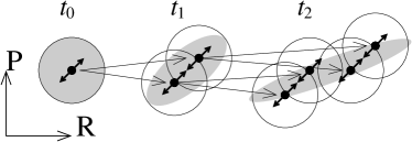
Figure 1: The branching of the wave packet in AMD/D is schematically shown for a free nucleon. The $\leftrightarrow$ symbols show the fluctuation to the wave packet centroids. Light gray region shows the exact time evolution of the Wigner function $\bar{f}$.

The light gray region in Fig. 1 shows the exact time evolution of the Wigner function $\bar{f}(\mathbf{r},\mathbf{p},t)$ for a free nucleon with the initial condition of a Gaussian wave packet at $t_{0}$. The spatial distribution increases as the time progresses, while the momentum distribution does not change at all. Due to the Liouville theorem, the phase space volume is conserved, which is the semiclassical analogue of the fact that $\bar{f}(\mathbf{r},\mathbf{p},t)$ corresponds to a pure state $\psi(\mathbf{r},t)$. At the initial time $t_{0}$, the Wigner function is diffusing in the direction of the $\leftrightarrow$ symbol in Fig. 1 and shrinking in the other direction. If AMD/D is applied to this situation, the diffusion is taken into account as branching by giving fluctuation to the wave packet centroid in the $\leftrightarrow$ direction, while the shrinking is ignored. At another time, $t_{1}$ or $t_{2}$, each of the branched wave packets is treated in the same way as the initial wave packet at $t_{0}$ (except for the different centroid value), without any influence of the history of the wave packet and the existence of the other branches. Namely, the fluctuation always has the same property for an free nucleon, and therefore both the spatial and the momentum distributions increase as the time progresses. Consequently the coherent Wigner function $\bar{f}(\mathbf{r},\mathbf{p},t)$ cannot be reproduced if AMD/D is applied. Generally speaking, decoherence increases the width of the phase space distribution.

In the practical calculations of nuclear reactions, the above problem for a free nucleon is not so serious because the dynamics of free nucleons is not of our interest, and it is usually sufficient to describe an emitted nucleon as moving on a straight line (or on a Coulomb trajectory) as a classical particle. Therefore, in Refs. ONOh ; ONOi the branching was switched off for isolated nucleons. For example, the switching-off condition adopted in Ref. ONOi is

$$\sum_{i}\theta\Bigl{(}1.75-|\Re(\mathbf{Z}_{i}-\mathbf{Z}_{k})|\Bigr{)}\leq 10$$ (51a)

and

$$\biggl{|}\sum_{i}\theta\Bigl{(}1.75-|\Re(\mathbf{Z}_{i}-\mathbf{Z}_{k})|\Bigr{)}\Re(\mathbf{Z}_{i}-\mathbf{Z}_{k})\biggr{|}\leq 5.$$ (51b)

This condition switches off the branching for the nucleons in small clusters with $A_{\text{c}}\lesssim 10$ as well as emitted nucleons.

Not only the branching is switched off for isolated nucleons, but also each isolated nucleon is regarded as having a definite momentum value without the internal distribution of the Gaussian wave packet. This interpretation is consistent to the definition of the Hamiltonian [Eq. (43)] where the zero-point oscillation kinetic energies of isolated nucleons have been subtracted. Therefore, we can get reasonable results even with AMD/D if the switching-off condition is appropriately chosen so that the branching is switched off (at $t_{2}$ in Fig. 1 for example) when the momentum centroid has got the appropriate amount of the fluctuation corresponding to the internal momentum distribution of the initial wave packet.

However, it will not be easy to find the switching-off condition that works for all situations. The condition of Eq. (51) may not work well for the reaction systems which have not been studied. When a big system is expanding slowly, for example, the switching-off will not take place for a long time, and then the branching will continue too long for the AMD/D method to reproduce the mean field prediction. In fact, we will show in Sec. III that the AMD/D method with the switching off condition (51) seems to overestimate the diffusion effect in a rather slowly expanding big system. Therefore we want such a new scheme of branching that we have no ambiguity of introducing any switching-off condition.

II.3.4 AMD/DS

Now we introduce a new scheme of decoherence by taking the choice of a large coherence time $\tau$ and a short time scale for mean field branching $\tau_{\text{mf}}=0$. We will call this model AMD/DS because the wave packet shrinking (S) effect in the mean field propagation [Eq. (4) or Eq. (17)] is reflected in the dynamics as well as the diffusion (D) effect with the choice of a finite $\tau$. The explicit definition of $\tau$, which depends on two-nucleon collisions, will be given later.

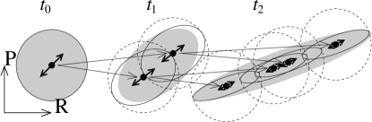
Figure 2: The branching of the wave packet in AMD/DS is schematically shown for a free nucleon. Light gray region shows the exact time evolution of the Wigner function $\bar{f}$. Each of the solid ellipses shows the shrunken shape $g(\mathbf{r},\mathbf{p};X(t),S(t))$ in each branch, while the dashed circles show the wave packets with the original width. The $\leftrightarrow$ symbols schematically show the magnitude and the direction of the fluctuation to the wave packet centroids.

AMD/DS provides us a one-body dynamics similar to that in mean field models, as expected from the fact that the coherent mean field propagation is respected by the choice of a large coherence time $\tau$. Figure 2 illustrates how our formulation in Sec. II.2 works in the simplest example of a free nucleon. The light gray region is identical to that in Fig. 1, showing the exact time evolution of the Wigner function $\bar{f}(\mathbf{r},\mathbf{p},t)$ with the initial condition of a Gaussian packet at the time $t_{0}$. The wave packet diffusion effect, $[(\delta/\delta t)S(t)]_{+}$ defined by Eq. (24), is taken into account as before by giving the fluctuation to the wave packet centroid $X(t)=(\mathbf{R}(t),\mathbf{P}(t))$ in Eq. (26) with the property of the fluctuation given by Eq. (25). On the other hand, the shrinking effect is reflected to the shape matrix $S(t)$ by the equation of motion (27). The ellipse with a solid line in each branch in Fig. 2 represents the deformed and shrunken shape of $g(\mathbf{r},\mathbf{p};X(t),S(t))$. It should be noted that the eigenvalues of $S(t)$ do not exceed the original wave packet width $\frac{1}{4}$ (shown by dotted circles in Fig. 2) since the diffusion beyond that width is considered by the fluctuation to the centroid. The exact Wigner function $\bar{f}(\mathbf{r},\mathbf{p},t)$ is reproduced by the mean average of the elliptic shapes $g(\mathbf{r},\mathbf{p};X(t),S(t))$ as defined by Eq. (18).

A general difference between AMD/DS and AMD/D is that the phase space diffusion is weaker in AMD/DS than in AMD/D, reflecting the different strength of decoherence. Mathematically, this difference arises due to the property of the fluctuation to the wave packet centroids. Namely, the Vlasov equation (20) is applied to different $g(\mathbf{r},\mathbf{p};X(t),S(t))$ which has always a full width in AMD/D and has a shrunken shape in AMD/DS, and therefore the property of the fluctuation [Eq. (25)] is different. In general, AMD/DS has smaller strength of the fluctuation than AMD/D (except for the switching-off in AMD/D). In the case of the AMD/DS description of a free nucleon in Fig. 2, as the time progresses, the strength of the fluctuation gets smaller and smaller with the direction of the fluctuation also changing, and at $t=\infty$ the fluctuation ceases and the elliptic distribution $S(\infty)$ is completely shrunken to have a definite value of the momentum.

It is easily proved that, in some cases, the coherent time evolution of the Wigner function is reproduced exactly by AMD/DS as the mean average of the shrunken elliptic shapes $g(\mathbf{r},\mathbf{p};X(t),S(t))$, in spite of the Gaussian-Gaussian approximation adopted in Sec. II.2.2. This is the case not only for a free nucleon but also for a nucleon in a harmonic oscillator potential with arbitrary curvatures. In general cases, however, the reproduction is not exact because of the Gaussian-Gaussian approximation. In future, such an approximation may be removed if it turns out to be necessary, but in the present work we are satisfied with this agreement of AMD/DS, which ensures the approximate validity of AMD/DS in the extreme case when decoherence does not physically take place.

When the coherence time $\tau$ is long and the mean field branching time is short ($\tau_{\text{mf}}=0$), it is interesting to imagine the behavior of this model in nuclear collisions. We can expect that the mean field branching (namely, the stochastic fluctuation of the mean field) does not influence so much the global dynamics and the early dynamics in high density stage. For such aspects, AMD/DS will behave similarly to the mean field model because the coherence of the single particle wave functions is kept for a large time scale $\tau$. On the other hand, for the aspect of clusterization, AMD/DS with $\tau_{\text{mf}}=0$ will behave like usual molecular dynamics models, because the branched mean field $h[\Phi(Z(t))]$ is equivalent to the mean field in such models, and therefore it helps the formation of clusters each of which is bound by the branched mean field.

The policy of the scheme of AMD/DS is to take $\tau$ that is as large as possible. However, if a two-nucleon collision takes place, it will not make sense to keep the coherence of the single particle wave functions of collided nucleons. Therefore, we assume that decoherence takes place for a nucleon with some probability when it experiences a two-nucleon collision with another nucleon. [Therefore $\tau$, defined for each nucleon, is the time interval between two successive collisions related to it.] The probability $P_{\text{dec}}$ of decoherence at each two-nucleon collision is chosen to be

$$P_{\text{dec}}(E,\theta)=e^{-E(1-\cos\theta)/E_{0}},$$ (52)

where $E$ is the two-nucleon collision energy in the laboratory system for the two nucleons and $\theta$ is the scattering angle in the center-of-mass system for the two nucleons. The purpose of this probability is to reject the low momentum transfer cases where the scattered state has a significant overlap probability with the case of no collision. Note that the probability is related to the momentum transfer $\mathbf{q}^{2}=ME(1-\cos\theta).$ The parameter $E_{0}=15$ MeV is chosen in the present work. With this choice, decoherence takes place in most of the collisions between the nucleons from the different initial nuclei in the early stage of the reaction with the incident energy more than several ten MeV/nucleon, while decoherence seldom takes place within the initial nuclei and the produced clusters.

At the end, let us discuss on the method of the subtraction of the zero-point kinetic energies of the isolated nucleons in Eq. (43). This subtraction is consistent to the coherent one-body dynamics of AMD/DS, in that the shrunken shape $g(\mathbf{r},\mathbf{p};X(t),S(t))$ for an emitted nucleon eventually has a definite momentum and therefore the zero-point kinetic energy should not be counted in the conserved energy $\mathcal{H}$. However, when a nucleon is coming out of a nucleus, the zero-point energy subtraction plays as a repulsive force to the nucleon from the nucleus in spite of the fact that such a repulsion does not exist in the one-body dynamics in the mean field. It is possible to remove the repulsive effect by keeping the conserved energy $\mathcal{H}$ given by Eq. (43). This is easily done by formally adding a term to the fluctuation part in the equation of motion (39) by the replacement

$$\frac{\partial\mathcal{O}_{k}}{\partial Z_{j\tau}^{*}}\rightarrow\frac{\partial\mathcal{O}_{k}}{\partial Z_{j\tau}^{*}}+\delta_{jk}T_{0}\frac{\partial N_{\mathrm{F}}}{\partial Z_{j\tau}^{*}}.$$ (53)

Then the added term cancels the zero-point subtraction term in the deterministic part $\{\mathbf{Z}_{i},\mathcal{H}\}$ and thus the repulsive force mentioned above does not exist any longer. The replacement of Eq. (53) is done at any place where $\mathcal{O}_{k}$ appears, like in Eqs. (44) and (46). Therefore, the conserved energy is still $\mathcal{H}$ with the zero-point energy subtracted. The key of this trick is that the zero-point energy is converted to the translational motion of the nucleon in the old treatment while that energy is shared by all the nucleons in the new treatment with the replacement of Eq. (53).

III Effects in a Multifragmentation Reaction

In this section, we discuss the results for ${}^{129}\mathrm{Xe}+\mathrm{Sn}$ collisions at the incident energy $E/A=50$ MeV and the impact parameter range $0<b<4$ fm. A detailed and systematic analysis of this reaction system will be given in separate papers HUDAN-thesis ; FRANKLAND-bormio . The main purpose here is to make comparison of the two models of the quantum branching in AMD, one (AMD/D) with only the wave packet diffusion effect and the other (AMD/DS) with the wave packet diffusion and shrinking effects, the latter effect being a consequence of the coherent mean field propagation for a finite coherence time $\tau$. From the character of these models, as discussed in the previous section, we expect that differences should be found in the diffusion property of nucleons in nuclear matter and the global one-body dynamics.

Many events with various impact parameters in the range of $0<b<4$ fm were produced by solving the stochastic equation of motion given in Sec. II.2. The triple loop approximation ONOi was used in order to save the computation time. The Gogny force GOGNY was used as the effective interaction. In the calculation of AMD/DS, we use the new treatment of the subtraction of the zero-point kinetic energies of nucleons and clusters given at the end of Sec. II.3.4, while AMD/D calculation is done with the old treatment of the zero-point subtraction, unless otherwise stated. In addition to the equation of motion, the two-nucleon collision effect was introduced in the usual stochastic way ONOab ; ONOd . The two-nucleon collision cross section adopted here is given by

$$\sigma(E,\rho)=\min\biggl{(}\sigma_{\text{LM}}(E,\rho),\ \frac{100\ \text{mb}}{1+E/(200\ \text{MeV})}\biggr{)},$$ (54)

where $\sigma_{\text{LM}}(E,\rho)$ is the cross section given by Li and Machleidt LiMachleidt from Dirac-Brueckner calculations using the Bonn nucleon-nucleon potential. This cross section depends on the two-nucleon collision energy $E$ and the density around the collision point $\rho$. It also depends on the isospins of the colliding nucleons. The temperature in the parameterization by Li and Macheit was, however, replaced by zero. A low energy cut has been introduced in the adopted cross section, though its effect on the final results has turned out to be unimportant. For the angular distribution, we use the same parameterization as in Ref. ONOd .

The calculation of each event was started by putting two nuclei with a distance 12 fm and boosting them at the time $t=0$. The AMD calculation was continued until $t=300$ fm/$c$, at which we assume the thermal equilibrium of each produced fragment and calculate its decay by using a statistical decay code MARUb which is based on the sequential binary decay model by Pühlhofer PUHLHOFER .

Figure 3: The time evolution of the density in the center of mass system projected on to the reaction plane, in a typical event of the ${}^{129}\mathrm{Xe}+\mathrm{Sn}$ collision at 50 MeV/nucleon, from $t=0$ to $t=225$ fm/$c$. The beam direction is parallel to the horizontal axis, and the impact parameter of this event is 3.4 fm. The size of the shown area is $60\ \text{fm}\times 60\ \text{fm}$. This is a result of the calculation with AMD/DS.

Figure 3 shows the time evolution of a typical event with the impact parameter $b=3.4$ fm. It appears that a system is formed, which, after a maximum compression around $t\sim 45$ fm/$c$, expands and many clusters appear around $t\sim 100$ fm/$c$. The expansion is stronger in the beam direction than in the transverse directions, which means that the initial nuclei do not stop completely even in such central collisions. Therefore, another possible interpretation may be that the initial two nuclei are passing each other with large dissipation and breaking up into clusters. However, the mixing of the wave packets from the two nuclei is considerable. On the average, 87 nucleons from the projectile ${}^{129}\mathrm{Xe}$ nucleus come out to the forward direction ($p_{z}>0$ in the center-of-mass system), while the other 42 nucleons from the projectile nucleus appear in the backward direction. This corresponds to around 67%-33% sharing of the projectile nucleons in forward-backward directions, to be compared with 50%-50% for full mixing or 100%-0% for no mixing at all. These qualitative features do not depend so much on the choice of the models of the quantum branching, though the event of Fig. 3 was obtained with AMD/DS.

The same reaction system has been studied by Nebauer et al. with the quantum molecular dynamics (QMD) INDRA . A serious problem of their QMD result is that too large projectilelike and targetlike fragments are produced even in the central collisions ($E_{\text{trans}}>450$ MeV). Consequently the QMD calculation largely overestimates the yield of the big clusters with $Z\gtrsim 20$, as shown in Fig. 7 of Ref. INDRA . This problem of the spurious binary feature is qualitatively similar to the problem which has ever encountered in the AMD calculation by Ono and Horiuchi for the ${}^{40}\mathrm{Ca}+{}^{40}\mathrm{Ca}$ collisions at 35 MeV/nucleon ONOh . This problem in AMD has been solved in Ref. ONOh by the stochastic incorporation the wave packet diffusion effect which allows the mixing and/or breakup of the initial nuclei. In fact, the present AMD calculation do not show the binary feature as strong as in the QMD calculation, which can be seen in Fig. 3 and in the cluster charge distribution to be shown later. The fermionic nature may also be important to solve the problem of QMD. Papa et al. have shown in Ref. PAPA that the spurious binary feature disappears when they introduce the fermionic nature into QMD in a stochastic way.

Figure 4: Time evolution of the transverse radius $\langle R_{\perp}\rangle$ (solid lines) and the transverse momentum $\langle P_{\perp}\rangle$ (dashed lines) in ${}^{129}\mathrm{Xe}+\mathrm{Sn}$ collisions at 50 MeV/nucleon averaged for the impact parameter region $0<b<4$ fm. The results of AMD/D are shown by thin lines, while those of AMD/DS are shown by thick lines. Filled and open circles show $\langle R_{\perp}\rangle$ and $\langle P_{\perp}\rangle$, respectively, obtained by the origial AMD calculation applied to the intermediate states at $t=60$ fm/$c$ of the AMD/DS calculation.

We can expect that the early stage dynamics is not so sensitive to the model of quantum branching, because AMD/D and AMD/DS are equivalent for a short time scale and because the effective coherence time in AMD/DS is short due to many two-nucleon collisions. In fact, it is seen in the part of $t\lesssim 60$ fm/$c$ in Fig. 4, which shows the time dependence of the two quantities

$$\langle R_{\perp}\rangle =\biggl{\langle}\frac{1}{A}\sum_{i=1}^{A}\sqrt{R_{ix}^{2}+R_{iy}^{2}}\biggr{\rangle},$$ (55)

$$\langle P_{\perp}\rangle =\biggl{\langle}\frac{1}{A}\sum_{i=1}^{A}\sqrt{P_{ix}^{2}+P_{iy}^{2}}\biggr{\rangle},$$ (56)

characterizing the transverse expansion. We use the transverse components of the physical positions $\mathbf{R}_{i}$ and the physical momenta $\mathbf{P}_{i}$ defined by Eq. (12). The brackets stand for the averaging over the events with the impact parameter range $0<b<4$ fm. [We consider these quantities rather than the root mean square quantities in order to focus on the central part of the system where clusters are mainly produced.] The solid lines in Fig. 4 show the transverse radius $\langle R_{\perp}\rangle$ and the dashed lines show the average transverse momentum $\langle P_{\perp}\rangle$. The thin lines show the result of AMD/D, while the thick lines show the result of AMD/DS. We can see that the transverse momentum is produced in the early stage of the collision (before 40 or 50 fm/$c$). As expected, there is no significant difference between AMD/D and AMD/DS for the early stage dynamics $t\lesssim 60$ fm/$c$.

Now our interest is in the evolution of the expanding system which has been created by the early stage dynamics before $t\sim 60$ fm/$c$. In Fig. 4, we can see that an important deviation between the two models appears in the spatial radius $\langle R_{\perp}\rangle$ in later reaction stage. The expansion velocity is slower in AMD/DS with the wave packet shrinking effect than in AMD/D without it. On the other hand, the transverse momentum, which is almost constant for $t\gtrsim 60$ fm/$c$, is almost independent of the model of the quantum branching. It should be noted that the expansion is governed not only by the momentum centroids of wave packets but also by the property of the fluctuation to the wave packet centroids. The latter is the difference between the models, which can be naturally understood because the wave packet shrinking effect reduces the strength of the fluctuation to the wave packet centroids, as discussed in Sec. II.3.4. To see this effect more clearly, we also show, by filled and open circles in Fig. 4, the results of the original AMD without quantum branching. In order to avoid the influence of the different early stage dynamics, the original AMD was applied to the intermediate states at $t=60$ fm/$c$ of the AMD/DS calculation. We can see that the transverse expansion is very weak without quantum branching.

In order to get a deeper understanding, let us first consider how the expansion dynamics is described if a mean field model (such as TDHF) is applied. If the two-nucleon collision effect is negligible in the expanding system, most of the single particle wave functions will widely spread over the space. Clusters will not be produced in a mean field model but the global one-body distribution may be reliable. Due to the coherence of the mean field propagation, the nucleon position and the nucleon momentum are strongly correlated in the expanded system, in a similar way to the case considered in Fig. 2 for example. If we focus on a local part of the expanded system, each nucleon has a rather sharp momentum distribution like a classical particle. The main aim of AMD/DS is to have the same global one-body distribution as in mean field models, when averaged over the branches. The essential difference is that the mean field varies from branch to branch in the case of AMD, which is the reason why clusters are produced in AMD, though this difference will not affect so much on the global one-body distribution. When clusters are formed, however, each nucleon is localized in one of the clusters, and then it should have some momentum distribution that satisfies the uncertainty relation and the Pauli principle. If this momentum distribution is considered, the global momentum distribution will become wider than the mean field prediction. Now the question is whether this widening of the momentum distribution should be respected or the coherent mean field propagation should be respected. When we apply AMD/DS, the coherent mean field propagation is respected and the widening of the momentum distribution is not considered as far as the one-body dynamics is concerned. It may be possible that the wave packet localization does not change the global one-body dynamics through complicated many-body correlations which are out of the scope of the present models. On the other hand, when we take AMD/D, we respect the widening of the momentum distribution due to the localization of the wave packet as physical decoherence, which will increase the future expansion velocity. It is not possible to say a priori that one model is superior to the other. What we can say is that AMD/DS reproduces the mean field prediction more precisely then AMD/D. It is another problem not discussed here whether the mean field prediction is always reliable or not.

Figure 5: The partitioning of the total charge into the clusters at $t=300$ fm/$c$ (before calculating the statistical decay of excited clusters) in ${}^{129}\mathrm{Xe}+\mathrm{Sn}$ collisions at 50 MeV/nucleon with the impact parameter $0<b<4$ fm. The area of each sector represents $ZM(Z)$ summed over the specified region of $Z$, where $M(Z)$ is the multiplicity of clusters with charge $Z$. (a) The result of AMD/DS. (b) The result of AMD/D. (c) The result of the original AMD applied to the intermediate states at 60 fm/$c$ of the AMD/DS calculation. (d) The result of AMD/D for the impact parameter region $4<b<7$ fm.

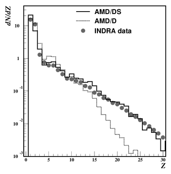
Figure 6: The charge distribution of the produced clusters in ${}^{129}\mathrm{Xe}+\mathrm{Sn}$ collisions at 50 MeV/nucleon with the impact parameter $0<b<4$ fm, after calculating the statistical decay of excited clusters and applying the experimental filter for the detector setup. Solid histogram shows the result of AMD/DS, while the dotted histogram shows the result of AMD/D. The INDRA experimental data INDRA are shown by bullets.

How does the different expansion velocity in the two models appear in the observables? As we have seen in Fig. 4, the difference does not appear in the global transverse momentum, and therefore the energy spectra are not good quantities to see the effect directly. The different expansion velocity is not due to the different momentum but due to the different strength of the spatial component of the fluctuation to the wave packet centroids. Therefore, we should look at the quantities which carry the information of the increase rate of the spatial radius. The cluster size distribution is one of such quantities because each cluster is formed by the nucleons with similar spatial positions and velocities. It has been shown that the cluster size decreases as the expansion velocity increases GRADY ; CHIKAZUMI . Figure 5 shows how the total 104 protons in the system are divided into clusters at $t=300$ fm/$c$ before calculating the statistical decay of excited clusters. The results of AMD/DS and AMD/D are shown in (a) and (b), respectively. It is clearly seen that heavy clusters are produced more abundantly in AMD/DS than in AMD/D, reflecting the different expansion velocity. In the case of the original AMD calculation circles) linked to the early stage dynamics of AMD/DS [shown in (c)], the produced clusters are much bigger than in AMD/DS, reflecting the very slow expansion. In Fig. 6, the final charge distribution after statistical decay is shown together with the INDRA data (bullets). The data and the calculated results can be directly compared, since the filter has been applied to the calculated events in order to take account of the properties of the detector system. The result of AMD/D has a serious problem that the multiplicity of the heavy clusters with $Z\gtrsim 15$ are underestimated. Instead of the heavy clusters, the relatively light clusters with $Z\sim 5,6$ are produced too abundantly. Therefore, it seems that the expansion is too fast in AMD/D. On the other hand, the reproduction by AMD/DS is quite satisfactory for the charge distribution of the clusters with $Z\geq 3$. These results suggest that it is reasonable to respect the mean field prediction of the expansion dynamics in this reaction system which consists of rather many nucleons and is expanding with a moderate velocity. However, AMD/DS has a problem of the overestimation of the proton multiplicity and the underestimation the $\alpha$ particle multiplicity. Probably this is a side effect of the fact that AMD/DS uses the mean field equation so faithfully that the light cluster emission is not respected compared to the nucleon emission. A special care ONOcoal will be necessary to explain the direct production of light clusters which have only one quantum bound state. The use of the semiclassical version of the mean field equation (the Vlasov equation) may also be one of the reasons why the nucleon emission is overestimated.

The above quantitative results can be affected, in principle, by the centrality selection method. In our calculation all the events with $0<b<4$ fm are considered as central events, while in experiment the central events are selected by using the sum of the transverse energies ($E_{\text{trans}}$) of observed light charged particles ($Z=1,2$). The experimental data in Fig. 6 were obtained by selecting the events with the condition $E_{\text{trans}}>450$ MeV INDRA . [These data are identical to those which have been shown by the histogram in Fig. 7 of Ref. INDRA in an arbitrary scale, while in our figure they are shown in the absolute scale.] Nebauer et al. have shown in QMD simulation that events with $4<b<6$ or 7 fm are also mixed in the selected events with $E_{\text{trans}}>450$ MeV (Fig. 3 of Ref. INDRA ). In order to estimate the effect of these semi-peripheral events, we show in Fig. 5(d) the charge partitioning obtained by AMD/D for $4<b<7$ fm. We can see that the character of clusterization in semi-peripheral events is not very different from the central events [Fig. 5(b)]. The difference between central and semi-peripheral events in AMD/D calculation [(b) and (d)] is not as big as the difference between AMD/D and AMD/DS in central events [(b) and (a)]. Therefore, a possible considerable mixture of semi-peripheral events in the data does not change our conclusion that too many small clusters are produced in AMD/D and that the reproduction is improved by respecting the coherence mean field propagation as in AMD/DS.

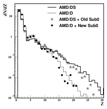
Figure 7: Similar to Fig. 6. Solid and dotted histograms are the same as in Fig. 6, showing the results of AMD/DS and AMD/D, respectively. The stars show the result of the calculation with AMD/DS combined with the old treatment of the zero-point kinetic energy subtraction. The bullets show the result of the calculation with AMD/D combined with the new treatment of the zero-point kinetic energy subtraction.

Finally, the dependence on the treatment of the zero-point kinetic energy subtraction is shown in Fig. 7 for the cluster charge distribution. As far as the AMD/D model of the quantum branching is used, the result is far from the experimental data irrelevantly to the treatment of the zero-point subtraction. In the result of AMD/DS, we can get a slightly better reproduction of data by using the new treatment of the zero-point subtraction given at the end of Sec. II.3.4. It should be noted that the new treatment of the zero-point subtraction is more consistent to the philosophy of the AMD/DS model of the quantum branching in that the mean field prediction of the one-body dynamics is respected.

IV Summary

In this paper, we have given a general framework which determines the many-body quantum dynamics by the combination of the coherent mean field propagation and the decoherence into branched wave packets. This framework contains the mean field description and the molecular dynamics description as specific cases. The model given by Refs. ONOh ; ONOi (AMD/D) corresponds to taking the zero coherence time ($\tau=0$) for the mean field propagation. In this scheme, the wave packet diffusion by the mean field propagation is respected by giving appropriate fluctuation to the wave packet centroids. However, the usual fluctuation was not able to describe the shrinking of the phase space distribution which could be respected only by keeping the coherence of the mean field propagation. On the other hand, we have shown in this paper that it is possible to implement a finite time duration $\tau$ of the coherent mean field propagation before decoherence, even though we still adopt a branching treatment. As a consequence, in the new model (AMD/DS), the shrinking of the phase space distribution is respected as well as the diffusion. AMD/DS reproduces the exact dynamics for a free nucleon and for a nucleon in a harmonic oscillator potential with arbitrary curvatures. In general cases, the branch-averaged one-body dynamics in AMD/DS should be much closer to the prediction by mean field models than in AMD/D. Nevertheless, by the choice of $\tau_{\text{mf}}=0$ for mean field branching, clusters can be formed in AMD/DS as well as in usual molecular dynamics models, because the mean field is calculated with localized wave packets in each branch. The two-nucleon collision effect is introduced as usual, and the decoherence into wave packets is assumed to take place when a nucleon experiences a two-nucleon collision with a substantial momentum transfer.

The difference of the decoherence scheme between the two models results in the different diffusion properties of nucleons in nuclear matter and the different global one-body dynamics. We have applied both models of AMD/D and AMD/DS to the ${}^{129}\mathrm{Xe}+\mathrm{Sn}$ collisions at 50 MeV/nucleon in the impact parameter range $0<b<4$ fm, where many clusters are produced from the expanding system with a moderate expansion velocity. The effect of the wave packet shrinking in AMD/DS certainly reduces the expansion velocity compared to AMD/D. Reflecting this difference in the expansion velocity, the charge distribution of the produced clusters strongly depends on the model of decoherence into branches. With AMD/DS, we have larger number of heavy clusters with $Z\gtrsim 15$ and smaller number of relatively small clusters with $Z\sim 5,6$ than with AMD/D. AMD/DS reproduces the INDRA experimental data much better than AMD/D, which suggests that the coherent mean field propagation for the one-body dynamics should be respected in this reaction system where a big system is expanding with a moderate expansion velocity. The detailed analysis of this reaction system based on the AMD calculations will be given in a separate paper.

However, we do not claim that AMD/DS is always superior to AMD/D or vice versa. These two models should be regarded as different schemes of approximation. AMD/DS respects the coherent mean field propagation, while AMD/D respects the existence of strong many-body correlations which causes the decoherence into branched wave packets. Although the decoherence has been considered in AMD/DS based on the two-nucleon collisions in this paper, it is also possible to have other many-body effects to cause decoherence, with which AMD/DS can be closer to AMD/D depending on the considered reaction systems. In future works, it will be important to investigate such possibilities.

- (1) J. Aichelin, Phys. Rep. 202, 233 (1991).
- (2) Toshiki Maruyama, A. Ono, A. Ohnishi and H. Horiuchi, Prog. Theor. Phys. 87, 1367 (1992).
- (3) A. Ono, H. Horiuchi, Toshiki Maruyama and A. Ohnishi, Phys. Rev. Lett. 68, 2898 (1992); A. Ono, H. Horiuchi, Toshiki Maruyama and A. Ohnishi, Prog. Theor. Phys. 87, 1185 (1992).
- (4) H. Feldmeier, Nucl. Phys. A515, 147 (1990).
- (5) G. F. Bertsch and S. Das Gupta, Phys. Rep. 160, 189 (1988).
- (6) W. Cassing, V. Metag, U. Mosel and K. Niita, Phys. Rep. 188, 363 (1990).
- (7) S. Ayik and C. Gregoire, Phys. Lett. B212, 269 (1988); Nucl. Phys. A513, 187 (1990).
- (8) J. Randrup and B. Remaud, Nucl. Phys. A514, 339 (1990).
- (9) A. Ono and H. Horiuchi, Phys. Rev. C53, 2958 (1996).
- (10) A. Ono, Phys. Rev. C59, 853 (1999).
- (11) D. Kiderlen and P. Danielewicz, Nucl. Phys. A620, 346 (1997).
- (12) M. Colonna and Ph. Chomaz, Phys. Letters, B436 1 (1998).
- (13) Toshiki Maruyama, K. Niita and A. Iwamoto, Phys. Rev. C53, 297 (1996).
- (14) A. Ohnishi and J. Randrup, Phys. Rev. Lett. 75, 596 (1995).
- (15) A. Ohnishi and J. Randrup, Ann. Phys. 253, 279 (1997).
- (16) A. Ono, H. Horiuchi and Toshiki Maruyama, Phys. Rev. C48, 2946 (1993).
- (17) Y. Kanada-En’yo, H. Horiuchi and A. Doté, Phys. Rev. C 60, 064304 (1999); and references therein.
- (18) W. H. Zurek, Phys. Today 44 (10), 36 (1991); and references therein.
- (19) R. Wada, K. Hagel, J. Cibor, J. Li, N. Marie, W. Q. Shen, Y. Zhao, J. B. Natowitz and A. Ono, Phys. Lett. B422, 6 (1998).
- (20) R. Wada, K. Hagel, J. Cibor, M. Gonin, Th. Keutgen, M. Murray, J. B. Natowitz, A. Ono, J. C. Steckmeyer, A. Kerambrum, J. C. Angélique, A. Auger, G. Bizard, R. Brou, C. Cabot, E. Crema, D. Cussol, D. Durand, Y. El Masri, P. Eudes, Z. Y. He, S. C. Jeong, C. Lebrun, J. P. Patry, A. Péghaire, J. Peter, R. Régimbart, E. Rosato, F. Saint-Laurent, B. Tamain, and E. Vient, Phys. Rev. C62, 034601 (2000).
- (21) Qin Zhi, A. Ono, Li Wenxin, Zhao Lili, Sun Tongyu, S. Ambe, Y. Ohkubo, M. Iwamoto, Y. Kobayashi, H. Maeda, F. Ambe, Z. Phys. A355, 315 (1996).
- (22) Y. Tosaka, A. Ono and H. Horiuchi, Phys. Rev. C60, 064613 (1999).
- (23) S. Hudan, Thèse de doctorat de l’Université de Caen, GANIL T01 07 (2001).
- (24) J. D. Frankland, A. Chbihi, S. Hudan, A. Mignon, A. Ono, for the INDRA and ALADIN collaborations, GANIL P 02 07, nucl-ex/0202026.
- (25) J. Dechargé and D. Gogny, Phys. Rev. C21, 1568 (1980).
- (26) G. Q. Li and R. Machleidt, Phys. Rev. C48, 1702 (1993); Phys. Rev. C49, 566 (1994).
- (27) F. Pühlhofer, Nucl. Phys. A280, 267 (1977).
- (28) R. Nebauer, J. Aichelin and the INDRA Collaboration, Nucl. Phys. A658, 67 (1999).
- (29) M. Papa, Toshiki Maruyama and A. Bonasera, Phys. Rev. C 64, 024612 (2001).
- (30) B. L. Holian and D. E. Grady, Phys. Rev. Lett. 60, 1355 (1988).
- (31) S. Chikazumi, Toshiki Maruyama, S. Chiba, K. Niita, and A. Iwamoto, Phys. Rev. C 63, 024602 (2001).
- (32) A. Ono, Proc. 7th International Conference on Clustering Aspects of Nuclear Structure and Dynamics, Rab, Croatia, June 14–19, 1999. (World Scientific, 2000) p. 294.