Nuclear weak-interaction processes in stars

Abstract

Recent experimental data and progress in nuclear structure modeling have lead to improved descriptions of astrophysically important weak-interaction processes. The review discusses these advances and their applications to hydrostatic solar and stellar burning, to the slow and rapid neutron-capture processes, to neutrino nucleosynthesis, and to explosive hydrogen burning. Special emphasis is given to the weak-interaction processes associated with core-collapse supernovae. Despite some significant progress, important improvements are still warranted. Such improvements are expected to come from future radioactive ion-beam facilities.

I Introduction

The weak interaction is one the four fundamental forces in nature. Like the other three – strong, electromagnetic and gravitation – it plays a keyrole in many astrophysical processes. This can be nicely illustrated by the observation that new insights into the nature of the weak interaction usually were closely followed by the recognition of their importance in some astrophysical context. Shortly after Pauli postulated the existence of the neutrino and Fermi developed the first theory of weak interaction Fermi (1934), Gamow and Schoenberg speculated about the possible role of neutrinos in stellar evolution and proposed their production in the star as an important source for stellar energy losses Gamow and Schoenberg (1940); Gamow (1941); Gamow and Schoenberg (1941). The development of the universal $V-A$ theory Feynman and Gell-Mann (1958) led Pontecorvo to realize that the bremsstrahlung radiation of neutrino pairs by electrons would be a very effective stellar energy loss mechanism Pontecorvo (1959). Just after the discovery of neutral weak current Freedman (1974), Mazurek (1975), and Sato (1975) recognized that this interaction would result in a sizable elastic scattering cross section between neutrinos and nucleons, leading to neutrino trapping during the core collapse of a massive star in a type II supernova.

The unified model of electroweak interaction Weinberg (1967); Salam (1968); Glashow et al. (1970) allows derivation of accurate cross sections for weak processes among elementary particles (i.e. electrons, neutrinos, quarks), but also for neutron and protons if proper formfactors are taken into account which describe the composite nature of the nucleons. However, the situation is different for weak interaction processes involving nuclei. Clearly, the smallness of the weak interaction coupling parameter allows treatment of these processes in perturbation theory, reducing the calculation basically to a nuclear structure problem. However, it has been the inability to adequately treat the nuclear many-body problem, which has – and in many cases still does - introduced a substantial uncertainty into some of the key weak interaction rates used in astrophysical simulations. However, the recent few years have witnessed a tremendous progress in nuclear many-body theory, made possible by new approaches and novel computer realizations of established models, but also by the availability of large computational capabilities. This progress allowed calculation of the rates for many of the stellar weak-interaction processes involving nuclei with significantly improved accuracy or for the first time. To actually know that the calculations are more reliable, implies the availability of experimental data which test, constrain and guide the theoretical models. Thus, the advances in modelling nuclear weak-interaction processes in stars also reflects the progress made by experimentalists in recent years which have succeeded to measure data which are relevant for the astrophysical applications discussed in this review either directly, e.g. half-lives for some short-lived nuclei on the r-process path Pfeiffer et al. (2001), or indirectly like the Gamow-Teller distributions for nuclei in the iron mass range Osterfeld (1992) which decisively constrain the nuclear models. Another recent experimental first has been the measurement of charged- and neutral-current neutrino-nucleus cross sections.

This review will report about progress in modelling nuclear weak-interaction processes and their possible implications for stellar evolution and nucleosynthesis. We will restrict ourselves to advances achieved by improved nuclear models, treating the weak interaction within the standard model. Of course, it has long been recognized (e.g. Sato and Sato, 1975) that stars can be used as laboratories for fundamental physics Raffelt (1996) searching for new weakly interacting particles or constraining exotic components of the weak interaction outside the standard model. This field is rapidly growing (see for example Raffelt, 1996, 1999, 2000; Corsico et al., 2001; Domínguez et al., 1999).

Our review is structured as follows. Following a very brief discussion of the required ingredients of the weak interaction we introduce the nuclear many-body models which have been used in the studies of the weak-interaction processes (section II). The remaining sections are devoted to the results of these calculations and their applications to astrophysics which include the solar nuclear reaction network and neutrino problem, the core collapse of massive stars, s- and r-process nucleosynthesis, neutrino nucleosynthesis, explosive hydrogen burning and type Ia supernovae.

Although generally quite important, weak-interaction processes constitute only a part of the many nuclear reactions occuring in stars. For recent reviews about other stellar nuclear reactions networks and nucleosynthesis the reader is referred to the comprehensive and competent work by (Wallerstein et al., 1997; Arnould and Takahashi, 1999; Boyd, 2000; Smith and Rehm, 2001).

II Theoretical description

II.1 Weak interactions in nuclei

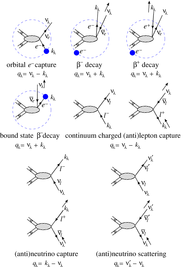
Figure 1: Semileptonic weak processes that occur during the evolution of stars. For each process the hadronic current is on the left and the leptonic current to the right. The dashed circle indicates a bound electron in the initial or final state. The four-momentum transfer $q_{\lambda}=(-\omega,\bm{q})$ for each process is given in terms of the charged lepton four-momentum $k_{\lambda}=(\epsilon,\bm{k})$ and the neutrino four-momentum $\nu_{\lambda}=(\nu,\bm{\nu})$. $\omega$, $\epsilon$, and $\nu$ represent the energy transfer, lepton energy and neutrino energy, respectively. In the case of antiparticles the directions of the momenta are show as an arrow close to the four-momentum label. The first row shows the usual decay modes in the laboratory. The second and third rows show processes that can occur under stellar conditions.

Processes mediated by the weak interaction in stars can be classified as leptonic (all interacting particles are leptons) and semileptonic (leptons interact with hadrons via the weak interaction). Leptonic processes can be straightforwardly computed using the standard electroweak model Grotz and Klapdor (1990). The calculation of semileptonic processes (i.e. neutrino-nucleus reactions, charged-lepton capture, and $\beta$-decay) is more complicated due to the description of the nuclear states involved. Fortunately the momenta of the particles turn out to be small compared with the masses of the $Z,W$ bosons. Thus it is sufficient to consider the semileptonic processes of interest in the lowest-order approximation in the weak interaction. Then the interaction can be described by a current-current Hamiltonian density:

$$\mathcal{H}(\bm{x})=-\frac{G}{\sqrt{2}}\mathcal{J}_{\mu}(\bm{x})j_{\mu}(\bm{x}),$$ (1)

where $G=G_{F}V_{ud}$ for charge-current processes and $G=G_{F}$ for neutral current processes, with $G_{F}$ the Fermi coupling constant and $V_{ud}$ the up-down entry of the Cabibbo-Kobayashi-Maskawa matrix Groom et al. (2000). $j_{\mu}(\bm{x})$ and $\mathcal{J}_{\mu}(\bm{x})$ are the weak leptonic and hadronic density operators Walecka (1975, 1995); Donnelly and Peccei (1979). The structure of the leptonic current $j_{\mu}(\bm{x})$ for a particular process is given by the standard electroweak model Weinberg (1967); Salam (1968); Glashow et al. (1970), and contains both, vector and axial-vector components. The standard model describes the hadronic current in terms of quark degrees of freedom. Since we are only interested in the matrix elements of $\mathcal{J}_{\mu}(\bm{x})$ in nuclei we need only to retain the pieces which involve $u$ and $d$ quarks. (The contribution from strange quarks is normally neglected, but see the discussion in section V.3.) As in nuclear physics the nucleons are treated as elementary spin-1/2 fermions, the Standard Model current is not immediately applicable. Moreover, nucleons in nuclei interact also via the strong interaction. It is then convenient to define an effective hadronic current using arguments of Lorentz covariance and isospin invariance of the strong interaction. The effective hadronic current can be decomposed into strong isoscalar ($T=0$) and isovector ($T=1$) components and contains both vector ($V$) and axial-vector ($A$) pieces. The weak charge-changing current is isovector with $M_{T}=\pm 1$ and can be written in a general form as:

$$\mathcal{J}_{\mu}=V_{\mu}^{1M_{T}}+A_{\mu}^{1M_{T}}.$$ (2)

This current governs processes (see figure 1) such as $\beta^{\pm}$-decay, $e$-capture, neutrino $(\nu_{l},l^{-})$ and anti-neutrino $(\bar{\nu}_{l},l^{+})$ reactions ($l=e,\mu$ or $\tau$). Under the conserved vector current (CVC) hypothesis Feynman and Gell-Mann (1958) the current $V_{\mu}^{1M_{T}}$ has a structure identical to the isovector part of the electromagnetic current. As a consequence of this hypothesis the weak charge-changing vector current is a conserved quantity. For the weak neutral current one has $M_{T}=0$ and, in general, both $T=0$ and $T=1$ pieces can occur. The general form of this current is

$$\mathcal{J}_{\mu}=\beta_{V}^{(0)}V_{\mu}^{00}+\beta_{A}^{(0)}A_{\mu}^{00}+\beta_{V}^{(1)}V_{\mu}^{10}+\beta_{A}^{(1)}A_{\mu}^{10}.$$ (3)

Assuming that the coupling constants are given by the Standard Model we have: $\beta_{V}^{(0)}=-2\sin^{2}\theta_{W}$, $\beta_{A}^{(0)}=0$, $\beta_{V}^{(1)}=1-2\sin^{2}\theta_{W}$, $\beta_{A}^{(1)}=1$ (Donnelly and Peccei, 1979, p. 25). $\theta_{W}$ is the weak mixing angle. The neutral current describes weak interactions such as neutrino $(\nu,\nu^{\prime})$ and anti-neutrino $(\bar{\nu},\bar{\nu}^{\prime})$ scattering.

The nuclear transitions that are induced by such weak currents (operators) involve initial and final states that are usually assumed to be eigenstates of angular momentum, parity, as well as isospin. It is then convenient to do a multipole expansion of the current operators. In that way one obtains the Coulomb, longitudinal, transverse electric and transverse magnetic multipoles defined in (Walecka, 1975, p. 136). The expressions necessary for the calculation of the processes shown in figure 1 can be obtained from references Walecka (1975); Donnelly and Peccei (1979) in terms of the multipole operators. In general the multipole operators are $A$-body nuclear operators (with $A$ the nucleon number). In practice, at the energy scales we are interested in, weak interactions perturb the nucleus only slightly, so that to a good approximation one-body components dominate most of the transitions. Two-body meson exchange currents and other many body effects are neglected (see Marcucci et al., 2001; Schiavilla and Wiringa, 2002, for a description of the nuclear current including two-body operators). It is further assumed that a nucleon in a nucleus undergoing a weak interaction can be treated as a free nucleon, which for the purpose of constructing interaction operators satisfies the Dirac equation. This latter approximation is known as the impulse approximation. For a single free nucleon, we have, using Lorentz covariance, conservation of parity, time-reversal invariance, and isospin invariance, the following general form for the vector and axial vector currents

$$\langle\bm{k}^{\prime}\lambda^{\prime};1/2m_{t^{\prime}}|V_{\mu}^{TM_{T}}|\bm{k}\lambda;1/2m_{t}\rangle=i\bar{u}(\bm{k}^{\prime}\lambda^{\prime})\left[F_{1}^{(T)}\gamma_{\mu}+F_{2}^{(T)}\sigma_{\mu\nu}q_{\nu}\right]u(\bm{k}\lambda)\langle 1/2m_{t^{\prime}}|I_{T}^{M_{T}}|1/2m_{t}\rangle,$$ (4a)

$$\langle\bm{k}^{\prime}\lambda^{\prime};1/2m_{t^{\prime}}|A_{\mu}^{TM_{T}}|\bm{k}\lambda;1/2m_{t}\rangle=i\bar{u}(\bm{k}^{\prime}\lambda^{\prime})\left[F_{A}^{(T)}\gamma_{5}\gamma_{\mu}-iF_{P}^{(T)}\gamma_{5}q_{\mu}\right]u(\bm{k}\lambda)\langle 1/2m_{t^{\prime}}|I_{T}^{M_{T}}|1/2m_{t}\rangle.$$ (4b)

Here, the plane-wave single nucleon states are labelled with the three-momenta $\bm{k}$ ($\bm{k}^{\prime}$), helicities $\lambda$ ($\lambda^{\prime}$), isospin $1/2$ and isospin projections $m_{t}$ ($m_{t^{\prime}}$). The momentum transfer, $q_{\mu}^{2}=q^{2}-\omega^{2}$, with $q=|\bm{q}|$, is defined in figure 1. Bold letters denote the three-momentum. The single-nucleon form factors $F_{X}^{(T)}=F_{X}^{(T)}(q_{\mu}^{2})$, $T=0,1$, $X=1,2,A,P$ (vector Dirac, vector Pauli, axial, and pseudoscalar) are all functions of $q_{\mu}^{2}$ Donnelly and Peccei (1979); Kuramoto et al. (1990); Beise and McKeown (1991); Musolf and Donnelly (1992). Second class currents are not included in equation (4). The isospin dependence in equations (4) is contained in

$$I_{T}^{M_{T}}\equiv\frac{1}{2}\times\left\{\begin{array}[]{ll}1&T=0,M_{T}=0\\ \tau_{0}&T=1,M_{T}=0\\ \tau_{\pm 1}=\mp\frac{1}{\sqrt{2}}(\tau_{1}\pm i\tau_{2})&T=1,M_{T}=\pm 1\end{array}\right.$$ (5)

To evaluate weak-interaction processes in nuclei, one needs matrix elements of the multipole operators between nuclear many-body states, labeled $|J_{i}M_{J_{i}};T_{i}M_{T_{i}}\rangle$ which are complicated nuclear configurations of protons and neutrons. Using the Wigner-Eckart theorem we can write the matrix element of an arbitrary multipole operator $\hat{T}_{JM_{J};TM_{T}}$ as Edmonds (1960)

$$\langle J_{1}M_{J_{1}};T_{1}M_{T_{1}}|\hat{T}_{JM_{J};TM_{T}}(q)|J_{2}M_{J_{2}};T_{2}M_{T_{2}}\rangle = (-1)^{J_{1}-M_{J_{1}}}\left(\begin{array}[]{ccc}J_{1}&J&J_{2}\\ -M_{J_{1}}&M_{J}&M_{J_{2}}\end{array}\right)$$ (8)

$$\times (-1)^{T_{1}-M_{T_{1}}}\left(\begin{array}[]{ccc}T_{1}&T&T_{2}\\ -M_{T_{1}}&M_{T}&M_{T_{2}}\end{array}\right)\langle J_{1};T_{1}|||\hat{T}_{J;T}(q)|||J_{2};T_{2}\rangle$$ (11)

where the symbol $|||$ denotes that the matrix element is reduced in both angular momentum and isospin. If we assume that the multipole operators are one-body operators, we can write Heyde (1994)

$$\langle J_{1};T_{1}|||\hat{T}_{J;T}(q)|||J_{2};T_{2}\rangle=\sum_{\alpha\alpha^{\prime}}\frac{\langle J_{1};T_{1}|||[a^{\dagger}_{\alpha^{\prime}}\otimes\tilde{a}_{\alpha}]_{J;T}|||J_{2};T_{2}\rangle}{\sqrt{(2J+1)(2T+1)}}\langle\alpha^{\prime}|||T_{J;T}(q)|||\alpha\rangle$$ (12)

with the sums extending over complete sets of single-particle wavefunctions $\alpha={n,l,j}$. The tensor product involves the single-particle creation operator $a^{\dagger}_{\alpha}\equiv a^{\dagger}_{\alpha;m_{j_{\alpha}}m_{t_{\alpha}}}$ and $\tilde{a}_{\alpha}\equiv(-1)^{j_{\alpha}-m_{\alpha}}(-1)^{1/2-m_{t_{\alpha}}}a_{\alpha;-m_{j_{\alpha}}-m_{t_{\alpha}}}$, with $a$ the destruction operator. The phase factor is introduced so that the operator $\tilde{a}$ transforms as a spherical tensor Edmonds (1960).

In practice the infinite sums in equation (12) are approximated to include a finite number of (hopefully) dominant terms. The number of terms to include depends both of the computed observable and the model used (Shell-Model, Random phase approximation, …). Typical nuclear models are non-relativistic, requiring a non-relativistic reduction of the single-particle operators; the respective expressions are given for example by Walecka (1975) and Donnelly and Peccei (1979). Donnelly and Haxton (1979) give the expressions for the single-particle matrix elements of these operators with harmonic oscillator wave functions. Donnelly and Haxton (1980) provide expressions for general wave functions.

The above discussion presents the general theory of semileptonic processes. However, in many applications the momentum transfers involved are small compared with the typical nuclear momentum $Q\approx R^{-1}$, with R the nuclear radius. In that case, the above formulas can be expanded in powers of $(qR)$ (long-wavelength limit) and one obtains the standard approximations to allowed (Gamow-Teller and Fermi) and forbidden transitions Behrens and Bühring (1982, 1971); Bambynek et al. (1977). In these limits the effect of the electromagnetic interaction on the initial or final charged lepton, that has been neglected in the above expressions, can be included Schopper (1966).

II.2 Nuclear models

As discussed in the previous section one of the basic ingredients for the evaluation of weak-interaction processes involving nuclei is the description of the nuclear many-body states. Moreover, the calculation of weak processes in stars have to account for the peculiarities of the medium (high temperatures and densities) and the presence of an electron plasma. When the temperatures and densities are small (for example during the r- and s-processes) weak transitions could be determined using the experimentally measured half-lives (in some cases one has to account for the presence of low lying isomeric states). However, as many of the very neutron-rich nuclei that participate in the r-process, are not currently accessible experimentally (see Pfeiffer et al., 2001, for recent experimental advances in the study of r-process nuclei), the necessary nuclear properties have to be extracted from theoretical models.

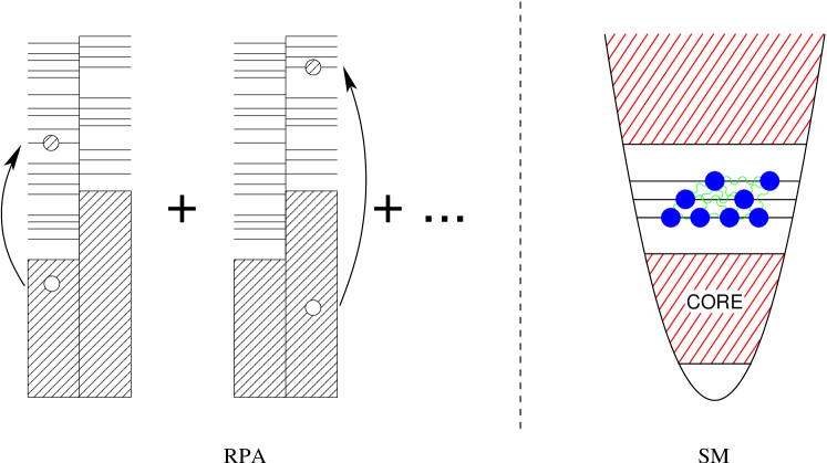
Figure 2: The most commonly used nuclear models for the calculation of weak processes in stars are the Random Phase Aproximation (RPA) and the Shell-Model (SM). In the RPA the basis states are characterized by particle-hole excitations around a given configuration (typically a closed-shell nucleus). In the SM, all the possible two-body correlations in a given valence space are considered. Excitations from the core or outside the model space are neglected, but his effect can be included perturbatively using effective interactions and operators.

As the degrees of freedom increase drastically with the number of nucleons, models of different sophistication have to be chosen for the various regions in the nuclear charts. Exact calculations using realistic nucleon-nucleon interactions, e.g. by Green’s Function Monte Carlo techniques, are restricted to light nuclei with mass $A\leq 10$ Carlson and Schiavilla (1998); Wiringa et al. (2000); Pieper (2002). As an alternative, methods based on effective field theory van Kolck (1999); Beane et al. (2001) have recently been developed for very light nuclei ($A\leq 3$) Marcucci et al. (2001); Park et al. (2001a, b); Marcucci et al. (2000). For heavier nuclei different approximations are required. In particular, restricted model spaces are used so that effective interactions and operators are necessary Hjorth-Jensen et al. (1995). For medium-mass nuclei ($A\leq 70$) the shell model is the method of choice Talmi (1993). This model explicitly treats all two-body correlations among a set of valance particles by a residual interaction. By diagonalizing the respective Hamiltonian matrix in the model space spanned by the independent particle states of the valence particles a quite satisfactory description of the ground state, the spectrum at moderate excitation energies and the electromagnetic and weak transitions among these states are obtained Caurier et al. (1994); Martínez-Pinedo et al. (1997). In recent times due to progress both in computer technology and programming techniques shell-model calculations are now possible in model spaces which seemed impossible only a few years ago; i.e. the diagonalization codes antoine or nathan developed by Etienne Caurier allow for complete calculations in the $pf$-shell where the maximum dimension currently attained is $2.3\times 10^{9}$ $M=0$ slater determinants for a complete diagonalization of ⁶⁰Zn Caurier (2002); Mazzocchi et al. (2001). To treat even larger model spaces in the diagonalization shell model, different schemes are required. One method is to expand the nuclear many-body wave functions in terms of a few symmetry-projected Hartree-Fock-Bogoliubov (HFB) type quasiparticle determinants Schmid et al. (1987, 1989); Schmid (2001). A novel approach, introduced by Honma et al. (1995) (see also Otsuka et al., 2001), employs stochastical methods to determine the most important Slater determinants in the chosen model space. As an alternative to the diagonalization method, the Shell Model Monte Carlo (SMMC) Johnson et al. (1992b); Koonin et al. (1997) allows calculation of nuclear properties as thermal averages, employing the Hubbard-Stratonovich transformation to rewrite the two-body parts of the residual interaction by integrals over fluctuating auxiliary fields. The integrations are performed by Monte Carlo techniques, making the SMMC method available for basically unrestricted model spaces. While the strength of the SMMC method is the study of nuclear properties at finite temperature, it does not allow for detailed nuclear spectroscopy.

The evaluation of nuclear matrix elements for the Fermi operator is straightforward. The Gamow-Teller operator connects Slater determinants within a model space spanned by a single harmonic oscillator shell ($0\hbar\omega$ space). The shell model is then the method of choice to calculate the nuclear states involved in weak-interaction processes dominated by allowed transitions as complete or sufficiently converged truncated calculations are nowadays possible for such $0\hbar\omega$ model spaces. The practical calculation of the Gamow-Teller distribution is achieved by adopting the Lanczos method Wilkinson (1965) as proposed by Whitehead (1980); (see also Poves and Nowacki, 2001; Langanke and Poves, 2000).

The calculation of forbidden transitions, however, involves nuclear transitions between different harmonic oscillator shells and thus requires multi-$\hbar\omega$ model spaces. These are currently only feasible for light nuclei where ab initio shell model calculations are possible Navrátil et al. (2000); Caurier et al. (2001). Such multi-$\hbar\omega$ calculations have been used for the calculation of neutrino scattering from ¹²C Hayes and Towner (2000); Volpe et al. (2000). However, for heavier nuclei one has to rely on more strongly truncated nuclear models. As the kinematics of stellar weak-interaction processes are often such that forbidden transitions are dominated by the collective response of the nucleus the Random Phase Appoximation Rowe (1968) is usually the method of choice (figure 2). Another advantage of this method is that, in contrast to the shell model, it allows for global calculations of these processes for the many nuclei often involved in nuclear networks. An illustrative example is the evaluation of nuclear half-lives based on the calculation of the GT strength function within the Quasiparticle RPA model Krumlinde and Möller (1984); Möller and Randrup (1990). The RPA method considers the residual correlations among nucleons via one particle one hole (1p-1h) excitations in large multi-$\hbar\omega$ model spaces. Compared to the shell model, the neglect of higher-order correlations renders the RPA method inferior for matrix elements between individual, non-collective states. A prominent example is the GT transition from the ¹²C ground state to the $T=1$ triad in the $A=12$ nuclei (e.g. Engel et al., 1996). While the shell model is able to reproduce the GT matrix element between these states Cohen and Kurath (1965); Warburton and Brown (1992), RPA calculations miss an important part of the nucleon correlations and overestimate these matrix elements by about a factor of 2 Kolbe et al. (1994); Engel et al. (1996). Recent developments have extended the RPA method to include the complete set of 2p-2h excitations in a given model space Drożdż et al. (1990). Such 2p-2h RPA models have, however, not yet been applied to semileptonic weak processes in stars. Moreover, the RPA allows for the proper treatment of the momentum-dependence in the different multipole operators, as it can be important in certain stellar neutrino-nucleus processes (see below), and for the inclusion of the continuum Buballa et al. (1991). Detailed studies indicate that standard and continuum RPA calculations yield nearly the same results for total semileptonic cross sections Kolbe et al. (2000). This is related to the fact that both RPA versions obey the same sumrules. The RPA has also been extended to deal with partial occupation of the orbits so that configuration mixing in the same shell is included schematically Rowe (1968); Kolbe et al. (1999b).

III Hydrogen burning and solar neutrinos

The tale of the solar neutrinos and their ‘famous’ problem took an exciting twist from its original goal of measuring the central temperature of the Sun to providing convincing evidence for neutrino oscillations, thus opening the door to physics beyond the standard model of the weak interaction. In 1946, Pontecorvo suggested Pontecorvo (1946, 1991) (later independently proposed by Álvarez, 1949) that chlorine would be a good detector material for neutrinos and subsequently in the 1950’s Davis built a radiochemical neutrino detector which observed reactor neutrinos via the ³⁷Cl($\nu_{e},e^{-})^{37}$Ar reaction Davis (1955). After the ³He($\alpha,\gamma){}^{7}$Be cross section at low energies had been found to be significantly larger than expected Holmgren and Johnston (1958) and, slightly later, the ⁷Be$(p,\gamma){}^{8}$B cross section at low energies had been measured Kavanagh (1960), it became clear that the Sun should also operate by what are now known as the ppII and ppIII chains and in that way generate neutrinos with energies high enough to be detectable by a chlorine detector Fowler (1958); Cameron (1958). This idea was then seriously pursued by Davis, in close collaboration with Bahcall. The observed solar neutrino flux turned out to be lower than predicted by the solar models (the original solar neutrino problem) Davis et al. (1968); Bahcall et al. (1968), triggering the development of further solar neutrino detectors, initiating the field of neutrino oscillation experiments and, after precision helioseismology data Christensen-Dalsgaard (2002) boosted the confidence in the solar models, finally culminating in the conclusive evidence for neutrino oscillations in the solar flux. A detailed recent review of the solar hydrogen burning and neutrino problem is given in Kirsten (1999).

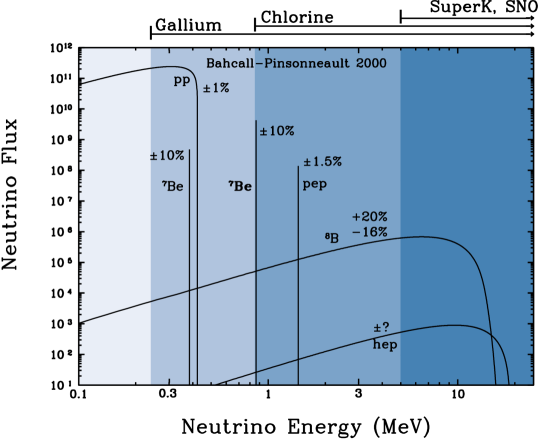
Figure 3: The energy spectrum of neutrinos predicted by the standard solar model Bahcall et al. (2001). The neutrino fluxes from continuum sources (like pp and ⁸B) are given in the units of number per cm² per second per MeV, while the line fluxes (e.g. ⁷Be) are given in number per cm² per second. The ranges of neutrino energies observable in the various detectors are indicated by arrows. The uncertainties in the various fluxes are given in percent (courtesy of J. N. Bahcall).

Reaction	Term	$\nu$ Energy
	(%)	(MeV)
$p+p\rightarrow{}^{2}\text{H}+e^{+}+\nu_{e}$	99.96	$\leq 0.423$
or
$p+e^{-}+p\rightarrow{}^{2}\text{H}+\nu_{e}$	0.44	1.445
${}^{2}\text{H}+p\rightarrow{}^{3}\text{H}+\gamma$	100
${}^{3}\text{He}+{}^{3}\text{He}\rightarrow\alpha+2p$	85
or
${}^{3}\text{He}+{}^{4}\text{He}\rightarrow{}^{7}\text{Be}+\gamma$	15
$\qquad{}^{7}\text{Be}+e^{-}\rightarrow{}^{7}\text{Li}+\nu_{e}$	15	$\left\{\begin{array}[]{r}0.863\ 90\%\\ 0.385\ 10\%\end{array}\right.$
$\qquad{}^{7}\text{Li}+p\rightarrow 2\alpha$
or
${}^{7}\text{Be}+p\rightarrow{}^{8}\text{B}+\gamma$	0.02
$\qquad{}^{8}\text{B}\rightarrow{}^{8}\text{Be}^{*}+e^{+}+\nu_{e}$		$<15$
$\qquad{}^{8}\text{Be}^{*}\rightarrow 2\alpha$
or
${}^{3}\text{He}+p\rightarrow{}^{4}\text{He}+e^{+}+\nu_{e}$	0.00003	$<18.8$

Table 1: The solar pp chains. The neutrino terminations are from the BP2000 solar model Bahcall et al. (2001). The neutrino energies include the solar corrections Bahcall (1997).

The Sun generates its energy from nuclear fusion reactions in the pp chain (see table 1), with a small contribution by the CNO cycle. Several of these reactions are mediated by the weak interaction, and hence create (electron) neutrinos which in the standard solar model can leave the Sun unhindered. The predicted flux of solar neutrinos on the surface of the earth is shown in figure 3. These predictions depend on the knowledge of the relevant nuclear cross sections at solar energies (a few keV) which, with the notable exception of the ³He(³He,2p)⁴He reaction Bonetti et al. (1999) which has been measured directly in the underground laboratory in the Gran Sasso, relies on the extrapolation of data taken at higher energies. As these reactions are all non-resonant, the extrapolations are quite mild and appear to be under control Adelberger et al. (1998). The cross section for the initial $p+p$ fusion reaction is so low that no data exist and the respective solar reaction rate relies completely on theoretical modelling. Nevertheless the underlying theory is thought to be under control and the uncertainty in this important rate is estimated to be about $1\%$ Kamionkowski and Bahcall (1994), based on potential model calculations, and it is probably even smaller if effective field theory is applied Park et al. (2001a); Park et al. (1998); Kong and Ravndal (2001). In the solar plasma the reaction rates are slightly enhanced due to screening effects Dzitko et al. (1995); Gruzinov and Bahcall (1998). The most significant plasma modification is found for the lifetime of ⁷Be with respect to electron capture where capture of continuum and bound electrons with the relevant screening corrections have to be accounted for Johnson et al. (1992a); Gruzinov and Bahcall (1998). It is generally believed that the ⁷Be$(p,\gamma){}^{8}$B reaction is the least known nuclear input in nuclear models. Although this reaction occurs in the weak ppIII chain, the decay of ⁸B is the source of the high-energy neutrinos observed by the solar neutrino detectors. Recent direct and indirect experimental methods have improved the knowledge of the ⁷Be$(p,\gamma)^{8}$B rate considerably (Davids et al. (2001) and references therein). While these data point to an astrophysical S-factor in the range of 18–20 eV b, a very recent direct measurement with special emphasis on the control and determination of the potential errors yielded a slightly larger value Junghans et al. (2001); Junghans and Snover (2002). The neutrino energy distribution arising from the subsequent ⁸B decay has been measured precisely by Ortiz et al. (2000). In principle, high-energy neutrinos are also produced in the ${}^{3}\text{He}+p$ fusion reaction which, however, occurs only in a weak branch in the solar pp cycles. Although the calculation of this cross section represents a severe theoretical challenge, it appears to be determined now with the required accuracy using state-of-the-art few-body methods Marcucci et al. (2000, 2001); Park et al. (2001a, b); Kong and Ravndal (2001).

The solar nuclear cross sections have been reviewed by Adelberger et al. (1998), including also the reactions occuring in the CNO cycle. Except for some discrepancies in the ¹⁴N(p,$\gamma)^{15}$O cross section at low energies Adelberger et al. (1998); Angulo and Descouvemont (2001), all relevant solar rates are sufficiently well known.

There are currently 5 solar neutrino detectors operating. Three of them, the homestake chlorine detector (Bahcall, 1989, p. 487), GALLEX Anselmann et al. (1992), and SAGE Abdurashitov et al. (1994)) can only observe charge-current (electron) neutrino reactions, while the two water Cerenkov detectors (Super-Kamiokande Fukuda et al. (1998b), SNO Boger et al. (2000)) also observe neutral-current events, which can be triggered by all neutrino flavors. All neutrino detectors have characteristic energy thresholds for neutrino detection, dictated by the various observation schemes; i.e. the detectors are blind for neutrinos with energies less than the threshold energy $E_{th}$. The pioneering chlorine experiment of Davis uses the ³⁷Cl($\nu_{e},e^{-})^{37}$Ar reaction as detector, with $E_{th}=814$ keV. Gallex and Sage detect neutrinos via ⁷¹Ga($\nu_{e},e^{-})^{71}$Ge with the threshold energy $E_{th}$=233.2 keV. In Super-Kamiokande (SK) solar neutrinos are identified by the observation of relativistic electrons produced from inelastic $\nu+e^{-}$ scattering. Due to high background at low energies, the observational threshold is set to $\sim 7$ MeV. SNO has an inner vessel of heavy water, surrounded by normal water. Like SK, this detector can also observe neutrinos via inelastic scattering off electrons. Additionally, and more importantly, SNO can also detect neutrinos by the dissociation of the deuteron in heavy water, with the threshold energy of order 6 MeV.

The threshold energies and the predicted solar neutrino fluxes are shown in figure 3. One notes that SK and SNO are only sensitive to ⁸B neutrinos (neglecting the weak $hep$ flux), the chlorine experiment detects mainly ⁸B (76$\%$ of the predicted flux by Bahcall et al. (2001)) and ⁷Be neutrinos, while Gallex and Sage can also observe neutrinos generated in the main solar energy source, the $p+p$ fusion reaction (54$\%$ of the predicted flux). It is important to note that the solar neutrino detectors have been calibrated, using known neutrino sources.

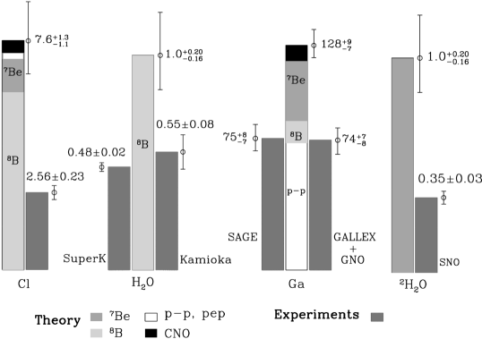
Figure 4: Comparison of the predicted solar neutrino fluxes Bahcall et al. (2001) for the various neutrino detectors with the observed fluxes. The unit for the chlorine detector (Cl) and the Gallium detectors (Ga) are Solar Neutrino Units (SNU) (see Bahcall, 1989), while for SNO and SK the comparison is in percentage of the predicted flux (courtesy of John N. Bahcall).

The original solar neutrino problem constitutes the fact that the earthbound detectors observe less neutrinos than predicted by the solar model. The current comparison is depicted in figure 4. Importantly, Sage and Gallex, in close agreement to each other, observe at least a neutrino flux which is consistent with the fact that the current solar luminosity is powered by the $p+p$ fusion reaction Hampel et al. (1999); Abdurashitov et al. (1999). With improved input (nuclear reaction rates, opacities, etc.) the solar models evolved and, as a milestone, passed the stringent test of detailed comparison to the soundspeed distribution derived from helioseismology Christensen-Dalsgaard et al. (1996). It became clear that the solution to the solar neutrino problem pointed to weak-interaction physics beyond the standard model. This line of reasoning was supported by the observation Heeger and Robertson (1996) that any solar model assuming standard weak-interaction physics leads to contradictions between the observed fluxes in the various detectors.

It has been speculated already for a long time Pontecorvo (1968) that the solution to the deficient observed neutrino flux lies in the possibility that neutrinos change their flavor on their way from the center of the Sun to the earthbound detectors. Neutrino oscillations can occur if the flavor eigenstates (the physical $\nu_{e},\nu_{\mu},\nu_{\tau}$ neutrinos) are not identical with the mass eigenstates $(\nu_{1},\nu_{2},\nu_{3}$) of the weak Hamiltonian, but rather are given by a unitary transformation of these states defined by a set of mixing angles. Importantly, oscillations between two flavor states can only occur if at least one of these states does not propagate with the speed of light implying that this neutrino has a mass different from zero; more precisely $\Delta m^{2}=m_{1}^{2}-m_{2}^{2}\neq 0$, where $m_{1,2}$ are the masses of the oscillating neutrinos. As all neutrino masses are assumed to be zero in the Weinberg-Salam model, the observation of neutrino oscillations opens the door to new physics beyond the standard model of weak interaction. Neutrino oscillations can occur for free-propagating neutrinos (vacuum oscillations). However, their occurence can also be influenced by the environment. In particular, it has been pointed out that the high-energy ($\nu_{e}$) solar neutrinos can, for a certain range of mixing angles and mass differences, transform resonantly into other flavors, mediated by the interaction of the $\nu_{e}$ neutrinos with the electrons in the solar plasma, resulting in matter-enhanced oscillations (the so-called MSW effect Wolfenstein, 1978; Mikheyev and Smirnov, 1986).

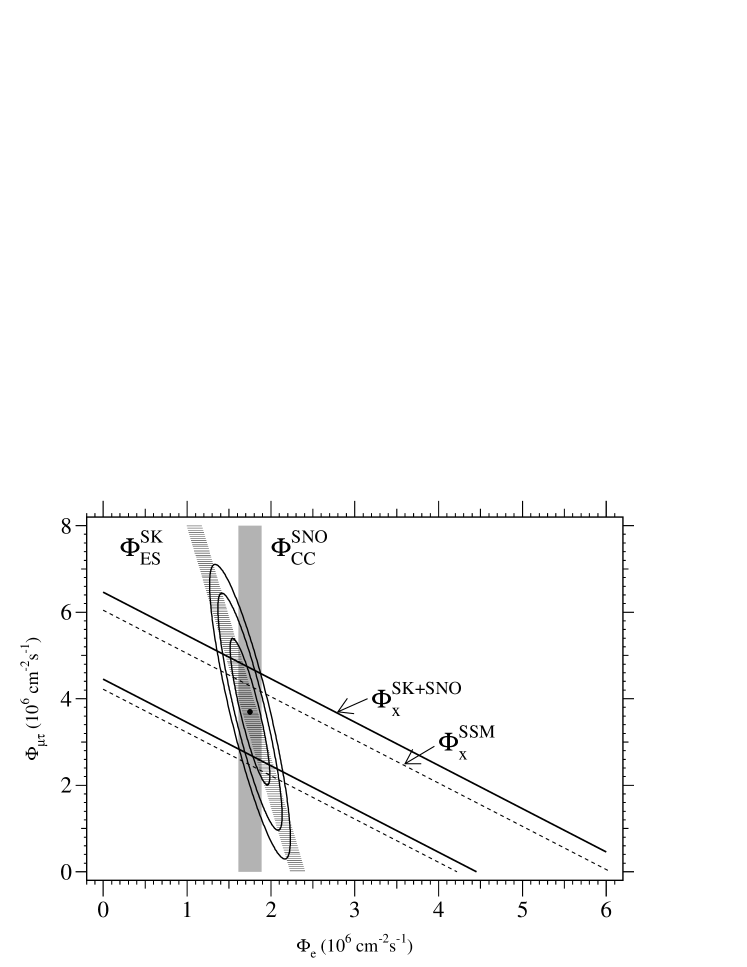
Figure 5: Flux of $\nu_{\mu,\tau}$ neutrinos vs. electron neutrinos as deduced from the SNO and SK ⁸B neutrino data. The diagonal bands show the total ⁸B flux as predicted by the standard solar model (SSM, dashed lines) Bahcall et al. (2001) and that derived from the SNO and SK measurements (solid lines). The intercepts with the axis represent $1\sigma$ errors (from Ahmad et al., 2001).

First clear evidence for neutrino oscillations was reported by the SK collaboration which observed a deficit of $\nu_{\mu}$-induced events from atmospheric neutrinos and could link this deficit to $\nu_{\mu}\rightleftarrows\nu_{\tau}$ oscillations Fukuda et al. (1998a); Fukuda et al. (1999). [Further evidence for neutrino oscillations has been given by the LSND collaboration Athanassopoulos et al. (1996, 1998). This result, however, was, for most of the allowed parameter space not confirmed by the Karmen experiment Armbruster et al. (1998a, b). The complete LSND result will be tested by the MiniBoone experiment which is currently under construction.] A clear link between neutrino oscillations and the solar neutrino problem has been presented recently by a combined analysis Ahmad et al. (2001) of the first SNO data with the precise SK data Fukuda et al. (2001). SNO measured the integrated event rate above the kinetic energy threshold $T_{\text{eff}}=6.75$ MeV (the electron energy threshold then is $E_{\text{th}}=T_{\text{eff}}+0.511$ MeV) for charged-current (CC) reactions on the deuteron and inelastic electron scattering (ES). As no evidence for a deviation of the spectral shape from the predicted shape under the no-oscillation hypothesis has been observed, the integrated rate could be converted into the measured ⁸B neutrino flux, resulting in $\Phi^{\text{CC}}_{\text{SNO}}(\nu_{e})=1.75\pm 0.07(\text{stat})\pm 0.12(\text{syst})\pm 0.05(\text{theor})\times 10^{6}$ cm^-2 s^-1, $\Phi^{\text{ES}}_{\text{SNO}}(\nu)=2.39\pm 0.34(\text{stat})\pm 0.15(\text{syst})\times 10^{6}$ cm^-2 s^-1. The SNO electron scattering flux result agrees with the more precise measurement from SK which yields $\Phi^{\text{ES}}_{\text{SK}}(\nu)=2.32\pm 0.03(\text{stat})\pm 0.08(\text{syst})\times 10^{6}$ cm^-2 s^-1. We note that the charged-current reaction can only be triggered by $\nu_{e}$ neutrinos at the energies of the solar neutrinos. Thus, from the measurement of the $\nu_{e}+D$ event rate, SNO has determined the solar $\nu_{e}$-flux arriving on earth stemming from the decay of ⁸B. On the other hand, neutrino-electron scattering can occur for all neutrino types, whereby the $\nu_{e}+e^{-}$ cross section is about seven times larger than the $\nu_{\mu,\tau}+e^{-}$ cross section. If no oscillations involving solar $\nu_{e}$ neutrinos occur, the SNO charged-current flux $\Phi^{\text{CC}}_{\text{SNO}}$ and the SK inelastic electron scattering flux $\Phi^{\text{ES}}_{\text{SK}}$ should be the same; that is excluded by 3.3 $\sigma$. [The exclusion is even slightly more severe if the recent revision of the $\nu_{e}+D$ cross section including radiative corrections is considered Kurylov et al. (2002).] If $\nu_{e}\rightleftarrows\nu_{\mu,\tau}$ oscillations occur, $\Phi^{\text{ES}}_{\text{SK}}$ should be larger than $\Phi^{\text{CC}}_{\text{SNO}}$ as it then contains additional neutral-current contributions from $\nu_{\mu,\tau}$ neutrinos. From a best fit to the SNO and SK data (see figure 5), this contribution has been determined as (with 1$\sigma$ uncertainty) $\Phi_{\mu,\tau}=3.69\pm 1.13\times 10^{6}$ cm^-2 s^-1 Ahmad et al. (2001), implying that the total solar flux is $\Phi_{\text{SNO}}^{\text{CC}}(\nu_{e})+\Phi(\nu_{\mu,\tau})=5.44\pm 0.99\times 10^{6}$ cm^-2 s^-1. This result agrees very nicely with the ⁸B neutrino flux predicted by the solar model Bahcall et al. (2001) ($5.05\times 10^{6}$ cm^-2 s^-1).

For years the measurement of the neutral-current $\nu$+D reaction at SNO has been anticipated as the ‘smoking gun’ for solar neutrino oscillations. After finishing this review, the first results of this milestone experiment have been published Ahmad et al. (2002a). They lead to the same conclusions as the earlier SNO results Ahmad et al. (2001) showing a clear excess of neutral-current over charged-current events, as expected if neutrino oscillations are the origin of the solar neutrino problem. Furthermore, the observed neutral-current event rate is again consistent with the prediction of the solar model Bahcall et al. (2001).

A global analysis of the latest solar neutrino data including the SNO charged-current rate favors matter-enhanced neutrino oscillations with large mixing angles Krastev and Smirnov (2002). Considering the recent constraints on the ⁷Be$(p,\gamma){}^{8}$B cross section and the respectively predicted ⁸B solar neutrino flux, vacuum oscillations are essentially excluded. A similar result is obtained by Bahcall et al. (2002) including the recent day-night asymmetry measured at SNO Ahmad et al. (2002b)

For more than 30 years the solar neutrino problem has been a demanding challenge for experimentalists and theorists, for nuclear, particle and astrophysicists alike. The challenge appears to be mastered, leading to new physics and without the need of the many desperate solution attempts put forward over the years.

IV Late-stage stellar evolution

IV.1 General remarks

Weak interactions play an essential role already during hydrostatic burning. Its importance lies in the fact that the neutrinos generated by these processes can leave the star unhindered, thus carrying away energy and hence cooling the star. While the consideration of energy losses by neutrinos is already required during hydrogen burning (see above), the heat flux in the early stages of stellar burning is predominantly by radiation. This changes, following helium burning, when the stellar temperatures reach $\sim 5\times 10^{8}$ K and neutrino-antineutrino pair production and emission becomes the leading energy loss mechanism. The respective cooling rate is a local property of the star depending on density $\rho$ and, very sensitively, on temperature $T$; i.e. the energy loss rate for $\nu{\bar{\nu}}$ emission scales approximately like $T^{11}$, implying that the hot inner regions of the star cool most effectively. However, the dominant nuclear reactions, occuring after helium burning, have even stronger temperature dependences. For example, the heat production $\epsilon$ in the ¹²C+¹²C or ¹⁶O+¹⁶O fusion reactions, which dominate hydrostatic carbon and oxygen burning, scales like $\epsilon\approx T^{22}$ and $\approx T^{35}$ around $T=10^{9}$ K. As a consequence of the temperature gradient in the stellar interior and the vast difference in the temperature sensitivity, nuclear reaction heating overcomes the neutrino energy loss in the center. However, in the cooler mantle region surrounding the core neutrino cooling dominates. The resulting entropy difference leads to convective instabilities (see Arnett, 1996). First attempts of modelling late-stage stellar burning and nucleosynthesis including a two-dimensional treatment of convection is reported in Baleisis and Arnett (2001).

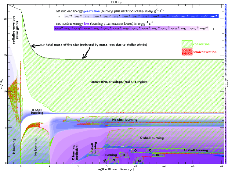
Figure 6: Energy history of a 22 $M_{\odot}$ star as a function of time until core collapse. The y-axis defines the included mass from the center. Hydrogen and helium core and shell burning are major energy sources. In the later burning stages, following oxygen core burning, neutrino losses related to weak processes in the stellar interior become increasingly important and can dominate over the nuclear energy production. Convection plays an important role in the envelope outside the helium burning shell, but also in shells during oxygen and silicon burning (from Heger and Woosley, 2001).

The importance of convection has, of course, already been noticed before and is accounted for in one-dimensional models within the so-called mixing-length theory Clayton (1968). It has been found that this convective transport is far more efficient at carrying energy and mixing the matter composition than radiation transport. For example, convection dominates the envelope region in massive stars during helium shell burning, as can be seen in figure 6 which shows the energy history of a 22 $M_{\odot}$ star Heger and Woosley (2001). The figure also identifies the various subsequent energy reservoirs of the star: hydrogen, helium, carbon, neon, oxygen, and silicon core and shell burning. However, the figure also demonstrates the importance of neutrino losses which, following oxygen core burning, can overcome the nuclear energy generation, except at the high temperatures in the very inner core. Obviously weak-interaction processes are crucial in this late epoch of massive stars. This is not only true for the star’s energy budget, but these processes can also alter the matter composition and entropy which, in turn, can affect the location and extension of convective shells, e.g. during oxygen and silicon burning, with subsequent changes in the stellar structure. Such effects have recently been observed after the improved shell-model weak-interaction rates (subsection III.2) have been incorporated into stellar models. (figure 6 is already based on these rates.)

IV.2 Shell-model electron capture and $\beta$ decay rates

The late evolution stages of massive stars are strongly influenced by weak interactions which act to determine the core entropy and electron to baryon ratio, $Y_{e}$, of the presupernova star, hence its Chandrasekhar mass which is proportional to $Y_{e}^{2}$. Electron capture reduces the number of electrons available for pressure support, while beta-decay acts in the opposite direction. Both processes generate neutrinos which, for densities $\rho\lesssim 10^{11}$ g cm^-3, escape the star carrying away energy and entropy from the core.

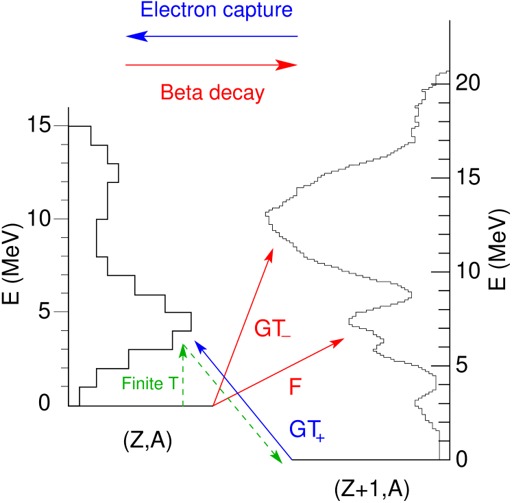
Figure 7: The figure shows schematically the electron capture and beta decay processes in the stellar environment. Electron capture proceeds by Gamow-Teller transitions to the GT₊ resonance. In the case of beta decay both the Fermi and Gamow-Teller resonances are typically outside of the $Q_{\beta}$ window, and hence are not populated in laboratory decays. Due to the finite temperature in stars excited states in the decaying nucleus can be thermally populated. Some of these states have strong GT transitions to low-lying states in the daughter nucleus. These states in the decaying nucleus are called “backresonances”.

Electron capture and beta decay during the final evolution of a massive star are dominated by Fermi and Gamow-Teller (GT) transitions. While the treatment of Fermi transitions (important only in beta decays) is straightforward, a correct description of the GT transitions is a difficult problem in nuclear structure. In the astrophysical environment nuclei are fully ionized so one has continuum electron capture from the degenerate electron plasma. The energies of the electrons are high enough to induce transitions to the Gamow-Teller resonance. Shortly after the discovery of this collective excitation Bethe et al. (1979) recognized its importance for stellar electron capture. The presence of the degenerate electron gas blocks the phase space for the produced electron in beta decay. Then the decay rate of a given nuclear state is greatly reduced or even completely blocked at high densities. However, due to the finite temperature excited states in the decaying nucleus can be thermally populated. Some of these states are connected by strong GT transitions to low-lying states in the daughter nucleus that with increased phase space can significantly contribute to the stellar beta decay rates. The importance of these states in the parent nucleus for beta-decay was first recognized by Fuller, Fowler and Newman (commonly abbreviated as FFN) who coined the term “backresonances” (see figure 7).

Over the years, many calculations of weak interaction rates for astrophysical applications have become available Hansen (1966, 1968); Mazurek (1973); Mazurek et al. (1974); Takahashi et al. (1973); Aufderheide et al. (1994c). For approximately 15 years though, the standard in the field has been the tabulations of Fuller, Fowler, and Newman (1980); Fuller, Fowler, and Newman (1982b, a); Fuller, Fowler, and Newman (1985). These authors calculated rates for electron capture, positron capture, beta-decay, and positron emission plus the associated neutrino losses for all the astrophysically relevant nuclei ranging in mass number from 21 to 60. Their calculations were based upon an examination of all available experimental information in the mid 1980s for individual transitions between ground states and low-lying excited states in the nuclei of interest. Recognizing that this only saturated a small part of the Gamow-Teller distribution, they added the collective strength via a single-state representation. Both, energy position and strength collected in this single state were determined using an independent particle model (IPM).

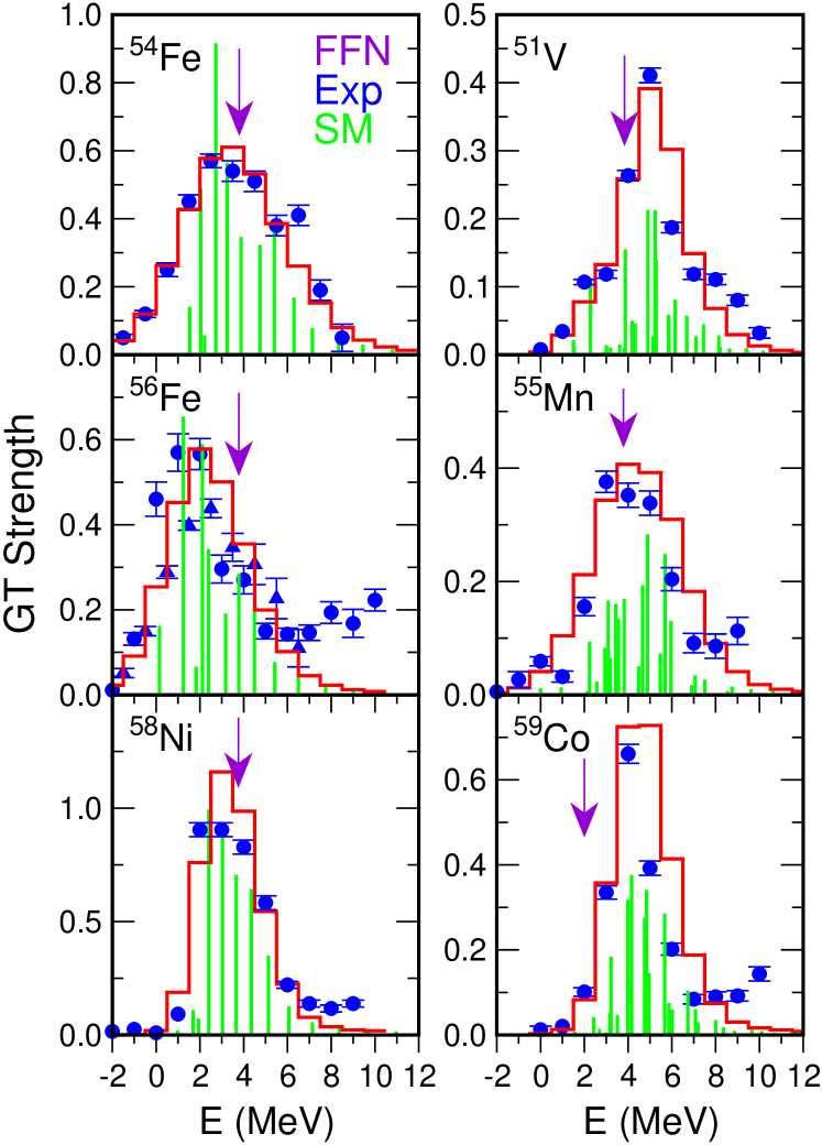
Figure 8: Comparison of shell model GT₊ distributions with experimental data Rönnqvist et al. (1993); El-Kateb et al. (1994); Alford et al. (1993) for selected nuclei. The shell model results (discrete lines) have been folded with the experimental resolution (histograms). The arrows indicate the positions where Fuller et al. (1982b) placed the GT resonance in their calculations of the stellar weak-interaction rates (adapted from Caurier et al., 1999).

Recent experimental data on GT distributions in iron group nuclei Alford et al. (1990, 1993); Williams et al. (1995); Vetterli et al. (1990); El-Kateb et al. (1994); Rapaport et al. (1983); Anderson et al. (1985, 1990); Rönnqvist et al. (1993) measured in charge exchange reactions Goodman et al. (1980); Osterfeld (1992), show that the GT strength is strongly quenched, compared with the independent particle model value, and fragmented over many states in the daughter nucleus. Both effects are caused by the residual interaction among the valence nucleons and an accurate description of these correlations is essential for a reliable evaluation of the stellar weak-interaction rates due to the strong phase space energy dependence, particularly of the stellar electron-capture rates. The shell model is the only known tool to reliably describe GT distributions in nuclei Brown and Wildenthal (1988). Indeed, Caurier et al. (1999) demonstrated that the shell model reproduces all measured GT₊ distributions (in this direction a proton is changed into a neutron, like in electron capture) for nuclei in the iron mass range very well and gives a very reasonable account of the experimentally known GT_- distributions (in this direction, a neutron is changed into a proton, like in $\beta$ decay). Further, the lifetimes of the $pf$-shell nuclei and their spectroscopy at low energies are simultaneously also described well. Figure 8 compares the shell model GT₊ distributions to the pioneering measurement performed at TRIUMF. These measurements had a typical energy resolution of $\sim 1$ MeV. Recently developed techniques, involving for example (${}^{3}\text{He},t$) Fujita et al. (1996) and ($d,{}^{2}$He) Wörtche (2001) charge-exchange reactions at intermediate energies, demonstrated in pilot experiments an improvement in the energy resolution by an order of magnitude or more. Again, the shell model calculations agree quite favorably with the improved data.

Several years ago, Aufderheide (1991) and Aufderheide et al. (1996, 1994c, 1993a, 1993b) pointed out that the interacting shell model is the method of choice for the calculation of stellar weak-interaction rates. Following the work by Brown and Wildenthal (1988), Oda et al. (1994) calculated shell-model rates for all the relevant weak processes for $sd$-shell nuclei ($A=17$–39). This work was then extended to heavier nuclei ($A=45$–65) by Langanke and Martínez-Pinedo (2001) based on shell-model calculations in the complete $pf$ shell. Following the spirit of FFN, the shell model results have been replaced by experimental data (energy positions, transition strengths) wherever available.

Weak interaction rates have also been computed using the proton-neutron quasiparticle RPA model Nabi and Klapdor-Kleingrothaus (1999b, a) and the spectral distribution theory Kar et al. (1994); Sutaria and Ray (1995)

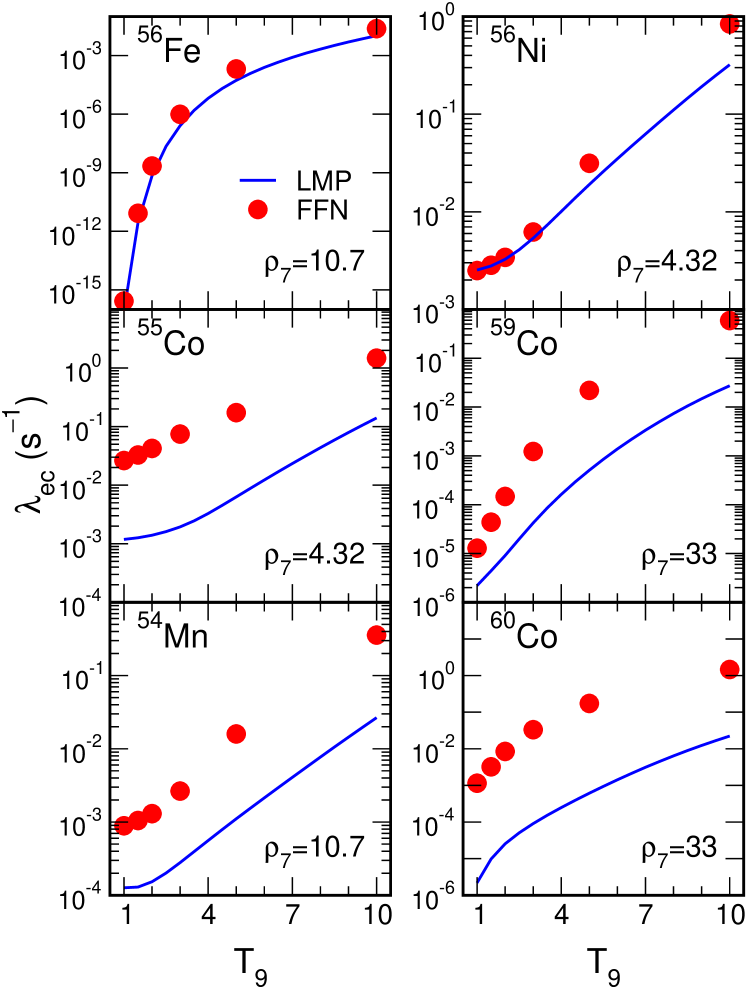
Figure 9: Shell model electron-capture rates as a function of temperature ($T_{9}$ measures the temperature in $10^{9}$ K) and for selected densities ($\rho_{7}$ defines the density in $10^{7}$ g cm^-3) and nuclei. For comparison, the FFN rates are given by the full points.

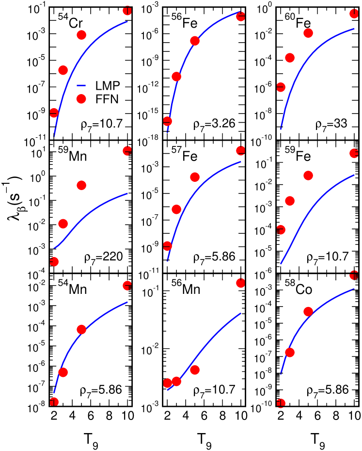
Figure 10: Shell model beta-decay rates as a function of temperature ($T_{9}$ measures the temperature in $10^{9}$ K) and for selected densities ($\rho_{7}$ defines the density in $10^{7}$ g cm^-3) and nuclei. For comparison, the FFN rates are given by the full points (from Martínez-Pinedo et al., 2000).

After oxygen burning, the important weak processes are electron captures and beta decays on nuclei in the iron mass range ($A\sim 45$–65). Conventional stellar models described these weak processes using the rates estimated by Fuller, Fowler, and Newman (1982b). These rates are compared to the shell model electron capture rates in figure 9 at relevant temperatures and densities. Importantly the shell model rates are nearly always lower than the FFN rates. Thus this difference represents a systematic trend, which is not expected to be washed out if the many nuclei in the stellar composition are considered. The difference is caused, for example, by the reduction of the Gamow-Teller strength (quenching) compared to the IPM value and a systematic misplacement of the Gamow-Teller centroid in nuclei with certain pairing structure Langanke and Martínez-Pinedo (2000). In some cases, experimental data, which were not available to FFN, but could be used by Langanke and Martínez-Pinedo (2001), led to significant changes. The FFN and shell-model beta decay rates are compared in figure 10, Martínez-Pinedo et al. (2000) discuss the differences between the two rate sets.

IV.3 Consequences of the shell model rates in stellar models

Heger et al. (2001a, b) have investigated the influence of the shell model rates on the late-stage evolution of massive stars by repeating the calculations of Woosley and Weaver (1995) keeping the stellar physics, except for the weak rates, as close to the original studies as possible. The new calculations have incorporated the shell-model weak interaction rates for nuclei with mass numbers $A=45$–65, supplemented by rates from Oda et al. (1994) for lighter nuclei. The earlier calculations of Weaver and Woosley (WW) used the FFN rates for electron capture and an older set of beta decay rates Mazurek (1973); Mazurek et al. (1974). As a side-remark we note that late-stage evolution of massive stars is quite sensitive to the still not sufficiently well known ¹²C($\alpha,\gamma)^{16}$O rate. The value adopted in the standard WW and in the Heger et al. models [$S(E=300\ \text{keV})=170$ keV b] agrees, however, rather nicely with the recent data analysis [$S(300)=165\pm 50$ keV b Kunz et al. (2001)] and the value derived from nucleosynthesis arguments by Weaver and Woosley (1993), [$S(300)=170\pm 20$ keV b].

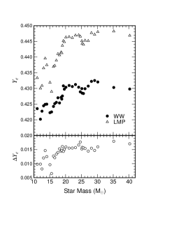
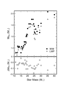
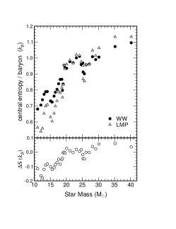
Figure 11: Comparison of the center values of $Y_{e}$ (left), the iron core sizes (middle) and the central entropy (right) for $11\text{--}40\ M_{\odot}$ stars between the WW models and the ones using the shell model weak interaction rates (LMP) (from Heger et al., 2001a). The lower parts define the changes in the 3 quantities between the LMP and WW models.

Figure 11 illustrates the consequences of the shell model weak interaction rates for presupernova models in terms of the three decisive quantities: the central electron-to-baryon ratio $Y_{e}$, the entropy, and the iron core mass. The central values of $Y_{e}$ at the onset of core collapse increased by 0.01-0.015 for the new rates. This is a significant effect. For example, a change from $Y_{e}=0.43$ in the WW model for a 20 $M_{\odot}$ star to $Y_{e}=0.445$ in the new models increases the respective Chandrasekhar mass by about 0.075 $M_{\odot}$. We note that the new models also result in lower core entropies for stars with $M\leq 20\ M_{\odot}$, while for $M\geq 20\ M_{\odot}$, the new models actually have a slightly larger entropy. The iron core masses are generally smaller in the new models where the effect is larger for more massive stars ($M\geq 20\ M_{\odot}$), while for the most common supernovae ($M\leq 20\ M_{\odot}$) the reduction is by about 0.05 $M_{\odot}$. [We define the iron core as the mass interior to the point where the composition becomes at least $50\%$ of iron group elements $(A\geq 48)$]. This reduction of the iron core mass appears to be counterintuitive at first glance with respect to the slower electron capture rates in the new models. It is, however, related to changes in the entropy profile during silicon shell burning which reduces the growth of the iron core just prior to collapse Heger et al. (2001a).

It is intriguing to speculate what effects these changes might have for the subsequent core collapse and supernova explosion. At first we note that in the current supernova picture Bethe (1990); Burrows (2000); Langanke and Wiescher (2001); Woosley et al. (2002) gravitation overcomes the resisting electron degeneracy pressure in the core, leading to increasing densities and temperatures. Shortly after neutrino trapping at densities of a few $10^{11}$ g cm^-3, an homologous core, which stays in sonic communication, forms in the center. Once the core reaches densities somewhat in excess of nuclear matter density (a few $10^{14}$ g cm^-3) the nuclear equation of state stiffens and a spring-like bounce is created triggering the formation of a shock wave at the surface of the homologous core Bethe (1990). This shock wave tries to traverse the rest of the infalling matter in the iron core. However, the shock loses its energy by dissociation of the infalling matter and by neutrino emission, and it is generally believed now that supernovae do not explode promptly due to the bounce shock. Probably, this happens in the ‘delayed mechanism’ Wilson (1985) where the shock is revived by energy deposition from the neutrinos generated by the cooling of the proto-neutron star, the remnant in the center of the explosion.

With the larger $Y_{e}$ values, obtained in the calculations with the improved weak rates, the core contains more electrons whose pressure acts against the collapse. It is also expected that the size of the homologous core, which scales like $\sim Y_{e}^{2}$ with the $Y_{e}$ value at neutrino trapping, should be larger. This, combined with the smaller iron cores, yields less material which the shock has to traverse. Furthermore, the change in entropy will affect the mass fraction of free protons, which in the later stage of the collapse contribute significantly to the electron capture. For presupernova models with masses $M<20\ M_{\odot}$, however, the number fraction of protons is very low ($\lesssim 10^{-6}$, Heger et al., 2001a) so that for these stars electron capture should still be dominated by nuclei, even at densities in access of $10^{10}$ g cm^-3. We will return to this problem below.

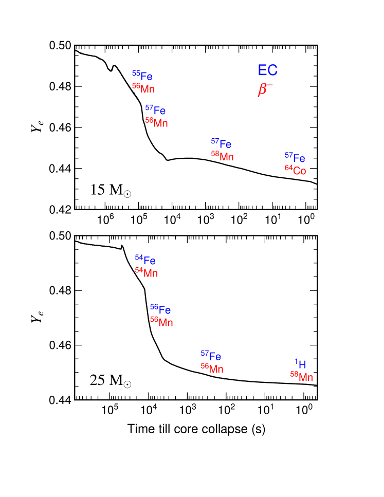
Figure 12: Evolution of the $Y_{e}$ value in the center of a 15 $M_{\odot}$ (upper part) and 25 $M_{\odot}$ (lower part) as a function of time until bounce. The most important $Y_{e}$-changing nuclei for the calculations adopting the shell model rates are indicated at different times, where the upper nucleus refers to electron capture and the lower to $\beta$-decay.

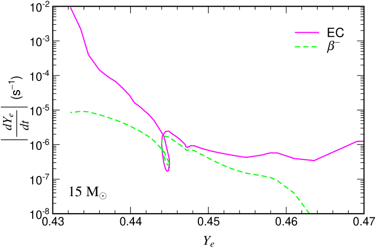
Figure 13: Comparison of the change of the $Y_{e}$ value with time, $|dY_{e}/dt|$ due to electron capture and beta decay in a 15 $M_{\odot}$ star. In general, the $Y_{e}$ value decreases with time during the collapse, caused by electron captures. The loops indicate that during this period beta-decay, which increases $Y_{e}$, dominates over electron capture.

To understand the origin of these differences it is illustrative to investigate the role of the weak-interaction rates in greater details. The evolution of $Y_{e}$ during the collapse phase is plotted in figure 12. Weak processes become particularly important in reducing $Y_{e}$ below 0.5 after oxygen depletion ($\sim 10^{7}$ s and $10^{6}$ s before core collapse for the 15 $M_{\odot}$ and 25 $M_{\odot}$ stars, respectively) and $Y_{e}$ begins a decline which becomes precipitous during silicon burning. Initially electron capture occurs much more rapidly than beta decay. As the shell model rates are generally smaller than the FFN electron capture rates, the initial reduction of $Y_{e}$ is smaller in the new models; the temperature in these models is correspondingly larger as less energy is radiated away by neutrino emission.

An important feature of the new models is demonstrated in figure 13. Beta decay becomes temporarily competitive with electron capture after silicon depletion in the core and during silicon shell burning (this had been foreseen in Aufderheide et al., 1994b). The presence of an important beta decay contribution has two effects. Obviously it counteracts the reduction of $Y_{e}$ in the core, but equally important, beta decays are an additional neutrino source and thus they add to the cooling of the core and a reduction in entropy. This cooling can be quite efficient as often the average neutrino energy in the involved beta decays is larger than for the competing electron captures. As a consequence the new models have significantly lower core temperatures than the WW models after silicon burning. At later stages of the collapse, beta decay becomes unimportant again as an increased electron chemical potential drastically reduces the phase space.

We note that the shell model weak interaction rates predict the presupernova evolution to proceed along a temperature-density-$Y_{e}$ trajectory where the weak processes are dominated by nuclei rather close to stability. Thus it will be possible, after next generation radioactive ion-beam facilities become operational, to further constrain the shell model calculations by measuring relevant GT distributions for unstable nuclei by charge-exchange reaction, where we like to point out again that the GT₊ distribution is also crucial for stellar $\beta$-decays. Figure 12 identifies those nuclei which dominate (defined by the product of abundance times rate) the electron capture and beta decay during various stages of the final evolution of 15 $M_{\odot}$ and 25 $M_{\odot}$ stars. Heger et al. (2001b) give an exhaustive list of the most important nuclei for both electron capture and beta decay during the final stages of stellar evolution for stars of different masses.

In total, the weak interaction processes shift the matter composition to smaller $Y_{e}$ values (see Fig. 12) and hence more neutron-rich nuclei, subsequently affecting the nucleosynthesis. Its importance for the elemental abundance distribution, however, strongly depends on the location of the mass cut in the supernova explosion. It is currently assumed that the remnant will have a baryonic mass between the iron core and oxygen shell masses Woosley et al. (2002). As the reduction of $Y_{e}$ occurs mainly during silicon burning, it is essential to determine how much of this material will be ejected. Another important issue is the possible long-term mixing of material during the explosion (e.g. Kifonidis et al., 2000). Changes of the elemental abundances due to the improved weak-interaction rates are rather small as the differences, compared to FFN, occur in regions of the star which are probably not ejected (however, for type Ia supernovae, see below). The weak interaction also determines the decay of the newly synthesized nuclei in supernova explosions. Some of them are proton-rich nuclei that decay by orbital electron capture, leaving atomic K-shell electron vacancies. The X-rays emitted can escape the supernova ejecta for sufficiently long-lived isotopes and can possibly be detected by the current generation of X-ray telescopes Leising (2001).

In dense stellar environment the electron capture rates have to be corrected for screening effects caused by the relativistically degenerate electron liquid. Such studies have been recently performed within the linear response theory Itoh et al. (2002) who find typical screening corrections of order a few percent.

V Collapse and post-bounce stage

The models, as we have described them above, constitute the so-called presupernova models. They follow the late-stage stellar evolution until core densities just below $10^{10}$ g cm^-3 and temperatures between 5 and 10 GK. (More precisely, Woosley and Weaver (1995) define the final presupernova models as the time when the collapse velocity near the edge of the iron core first reached 1000 km s^-1.) As we have stressed above, stellar evolution until this time requires the consideration of an extensive nuclear network, but is simplified by the fact that neutrinos need only be treated as a source for energy losses. This is no longer valid at later stages of the collapse. As neutrinos will eventually be trapped in the collapsing core and their interaction with the surrounding matter is believed to be crucial for the supernova explosion, computer simulations of the collapse, bounce and explosion necessitate a detailed time- and space-dependent bookkeeping of the various neutrino ($\nu_{e},\nu_{\mu},\nu_{\tau}$ neutrinos and their antiparticles) distributions in the core. Built on the pioneering work by Bruenn (1985), this is done by multi-group (neutrinos of different flavor and energy) Boltzmann neutrino transport Mezzacappa et al. (2001); Liebendörfer et al. (2001); Rampp and Janka (2000). Advantageously, the temperature during the collapse and explosion are high enough that the matter composition is given by nuclear statistical equilibrium without the need of reaction networks for the strong and electromagnetic interaction. The transition from a rather complex global nuclear network, involving many neutron, proton and $\alpha$ fusion reactions and their inverse, to a quasi-statistical equilibrium, in which reactions within mini-cycles are fast enough to bring constrained regions of the nuclear chart into equilibrium, to finally global nuclear statistical equilibrium is extensively discussed by Woosley (1986).

Presupernova models are the input for collapse and explosion simulations. Currently, one-dimensional models with sophisticated neutrino transport do not explode Mezzacappa et al. (2001); Liebendörfer et al. (2001); Rampp and Janka (2000), including first attempts with the presupernova models derived with the improved weak-interaction rates discussed above Messer et al. (2002). Explosions can, however, be achieved if the shock revival in the delayed mechanism is modelled by two-dimensional hydrodynamics allowing for more efficient neutrino energy transfer Herant et al. (1994); Burrows et al. (1995); Janka and Müller (1996). Thus the intriguing question arises: Are supernova explosions three-dimensional phenomena requiring convective motion and perhaps rotation and magnetic fields? Or do one-dimensional models fail due to incorrect or insufficient nuclear physics input? Although first steps have been taken in modelling the multi-dimensional effects (for reviews and references see Janka et al., 2001; Woosley et al., 2002), these require extremely demanding and computationally challenging simulations. In the following we will briefly discuss some nuclear physics ingredients in the collapse models and their possible improvements.

The crucial weak processes during the collapse are Bruenn (1985); Rampp and Janka (2002); Burrows (2001):

$$p+e^{-} \rightleftarrows n+\nu_{e}$$ (13a)

$$n+e^{+} \rightleftarrows p+\bar{\nu}_{e}$$ (13b)

$$(A,Z)+e^{-} \rightleftarrows (A,Z-1)+\nu_{e}$$ (13c)

$$(A,Z)+e^{+} \rightleftarrows (A,Z+1)+\bar{\nu}_{e}$$ (13d)

$$\nu+N \rightleftarrows \nu+N$$ (13e)

$$N+N \rightleftarrows N+N+\nu+\bar{\nu}$$ (13f)

$$\nu+(A,Z) \rightleftarrows \nu+(A,Z)$$ (13g)

$$\nu+e^{\pm} \rightleftarrows \nu+e^{\pm}$$ (13h)

$$\nu+(A,Z) \rightleftarrows \nu+(A,Z)^{*}$$ (13i)

$$e^{+}+e^{-} \rightleftarrows \nu+\bar{\nu}$$ (13j)

$$(A,Z)^{*} \rightleftarrows (A,Z)+\nu+\bar{\nu}$$ (13k)

Here, a nucleus is symbolized by its mass number $A$ and charge $Z$, $N$ denotes either a neutron or a proton and $\nu$ represents any neutrino or antineutrino. In the early collapse stage, before trapping, these reactions proceed dominantly to the right. We note that, due to the generally accepted collapse picture (e.g. Bethe, 1990), elastic scattering of neutrinos on nuclei (13g) is mainly responsible for the trapping, as it determines the diffusion time scale of the outwards streaming neutrinos. Shortly after trapping, the neutrinos are thermalized by the energy downscattering, experienced mainly in inelastic scattering off electrons (13h). The relevant cross sections for these processes are readily derived Bruenn (1985). For elastic neutrino-nucleus scattering one usually makes the simplifying assumption that the nucleus has a $J=0^{+}$ spin/parity assignment, as appropriate for the ground state of even-even nuclei. The scattering process is then restricted to the Fermi part of the neutral current (pure vector coupling) Freedman (1974); Tubbs and Schramm (1975) and gives rise to coherent scattering; i.e. the cross section scales with $A^{2}$, except from a correction $\sim(N-Z)/A$ arising from the neutron excess. This assumption is, in principle, not correct for the ground states of odd-$A$ and odd-odd nuclei and for all nuclei at finite temperature, as then $J\geq 0$ and the cross section will also have an axial-vector Gamow-Teller contribution. However, the relevant GT₀ strength is not concentrated in one state, but rather fragmented over many nuclear levels. Thus, one can expect that the GT contributions to the elastic neutrino-nucleus cross sections are in general small enough to be neglected.

Reactions (13a) and (13c) are equally important, as they control the neutronization of the matter and, in a large portion, also the star’s energy losses. Due to their strong phase space sensitivity ($\sim E_{e}^{5}$), the electron capture cross sections increase rapidly during the collapse as the density (the electron chemical potential scales like $\sim\rho^{1/3}$) and the temperature increase. We already observed above that beta-decay is rather unimportant during the collapse due to Pauli-blocking of the electron phase space in the final state. We also noted how sensitively the electron capture rate on nuclei depends on a proper description of nuclear structure. As we will discuss now, this is also expected for this stage of the collapse, although the relevant nuclear structure issues are somewhat different.

V.1 Electron capture on nuclei

The new presupernova models indicate that electron capture on nuclei will still be important, at least in the early stage of the collapse. Although capture on free protons, compared to nuclei, is favored by the significantly lower Q-value, the number fraction of free protons $Y_{p}$, i.e. the number of free protons divided by the total number of nucleons, is quite low ($Y_{p}\sim 10^{-6}$ in the 15 $M_{\odot}$ presupernova model of Heger et al., 2001b). This tendency had already been observed before, but has been strengthened in the new presupernova models, where the $Y_{e}$ values are significantly larger and thus the nuclei present in the matter composition are less neutron-rich, implying lower Q-values for electron capture. Furthermore, the entropy is smaller in stars with $\lesssim 20\ M_{\odot}$, yielding a smaller fraction of free protons.

As the entropy is rather low Bethe et al. (1979), most of the collapsing matter survives in heavy nuclei. However, $Y_{e}$ decreases during the collapse making the matter composition more neutron-rich, hence energetically favoring increasingly heavy nuclei. In computer studies of the collapse, the ensemble of heavy nuclei is described by one representative which is generally chosen to be the most abundant in the nuclear statistical equilibrium composition. Due to a simulation of the infall phase Mezzacappa and Bruenn (1993a, b), such representative nuclei are ⁷⁰Zn and ⁸⁸Kr at different stages of the collapse Mezzacappa (2001).

In current collapse simulations the treatment of electron capture on nuclei is schematic and rather simplistic. The nuclear structure required to derive the capture rate is then described solely on the basis of an independent particle model for iron range nuclei, i.e., considering only Gamow-Teller transitions from $f_{7/2}$ protons to $f_{5/2}$ neutrons Bethe et al. (1979); Bruenn (1985); Mezzacappa and Bruenn (1993a, b). In particular, this model predicts that electron capture vanishes for nuclei with charge number $Z<40$ and neutron number $N\geq 40$, arguing that Gamow-Teller transitions are blocked by the Pauli principle, as all possible final neutron orbitals are already occupied in nuclei with $N\geq 40$ (closed $pf$ shell) Fuller (1982). Such a situation would, for example, occur for the two nuclei ⁷⁰Zn and ⁸⁸Kr with $(Z=30,N=40)$ and $(Z=36,N=52)$, respectively. It has been pointed out Cooperstein and Wambach (1984) that this picture is too simple and that the blocking of the GT transitions will be overcome by thermal excitation which either moves protons into $g_{9/2}$ orbitals or removes neutrons from the $pf$ shell, in both ways reallowing GT transitions. In fact, due to this ‘thermal unblocking’, GT transitions again dominate the electron capture on nuclei for temperatures of order 1.5 MeV Cooperstein and Wambach (1984). An even more important unblocking effect, which is already relevant at lower temperatures is, however, expected by the residual interaction which will mix the $g_{9/2}$ (and higher) orbitals with those in the $pf$ shell.

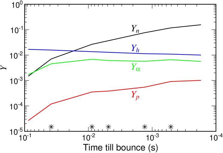
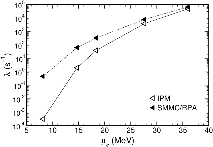
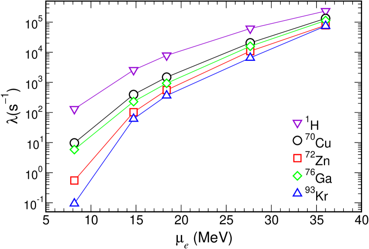
Figure 14: Electron capture rates on free proton and several representative nuclei as a function of electron chemical potential $\mu_{e}$ (lower panel). The rates have been determined for conditions during the infall phase Liebendörfer (2002): ($T,Y_{e},\rho_{11}$)=(0.846,0.429,0.102), (1.133,0.410,0.601), (1.259,0.400,1.186), (1.617,0.372,4.287), (2.000,0.349,10.063), where the temperature $T$ is given in MeV and $\rho_{11}$ measures the density in $10^{11}$ g cm^-3. The electron chemical potential increases during the infall, $\mu_{e}\sim\rho^{1/3}$. The middle panel compares the capture rates on ⁷⁸Ge in the independent particle model (IPM), in which Gamow-Teller transitions are Pauli-blocked, with the results obtained in the hybrid model (SMMC/RPA) which unblocks these transitions due to correlations and finite temperature effects. The rates have been calculated without neutrino final-state Pauli blocking which will become important at trapping densities. The upper panel shows the time evolution of the number abundances for neutrons $Y_{n}$, protons $Y_{p}$, $\alpha$-particles $Y_{\alpha}$ and heavy nuclei $Y_{h}$ calculated along the same stellar trajectory for which the rates have been calculated at selected points. These points are marked by asterisks (from Sampaio et al., 2002a).

A consistent calculation of the electron capture rates for nuclei with neutron numbers $N>40$ and proton numbers $20<Z<40$, including configuration mixing and finite temperature, is not yet feasible by direct shell model diagonalization due to the large model spaces and many states involved. It can, however, be performed in a reasonable way adopting a hybrid model: The capture rates are calculated within the RPA approach with partial occupation formalism, including allowed and forbidden transitions. The partial occupation numbers represent an ‘average’ state of the parent nucleus and depend on temperature. They are calculated within the Shell Model Monte Carlo approach at finite temperature Koonin et al. (1997) and include an appropriate residual interaction. Exploratory studies, performed for a chain of germanium isotopes ($Z=32$), confirm that the GT transition is not blocked for $N\geq 40$ and still dominates the electron capture process for such nuclei at stellar conditions Langanke et al. (2001a). This is demonstrated in figure 14, which compares electron capture rates for ⁷⁸Ge calculated within the hybrid model with the results in the independent particle model (IPM). For this nucleus ($N=46$) the rate in the IPM is given solely by forbidden transitions (mainly induced by $1^{-}$ and $2^{-}$ multipoles). However, correlations and finite temperature unblock the GT transitions in the hybrid model which increases the rate significantly. The differences are particularly important at lower densities (a few $10^{10}$ g cm^-3) where the electron chemical potential does not suffice to induce forbidden transitions.

We note again that many nuclei are present with similar mass abundances during the supernova collapse phase and that their relative abundances are approximately described by nuclear statistical equilibrium. Figure 14 shows the capture rates for several representative nuclei during the collapse phase, identified by the average charge and mass number of the matter composition following the time evolution of a certain ($M=0.6\ M_{\odot}$) mass trajectory Liebendörfer et al. (2001). (For the conditions shown in figure 14 ⁹³Kr and ⁷²Zn are examples of representative nuclei at $\rho_{11}=10.063$ and 0.601, respectively). The general trend of the rates reflects the competition of the two main energy scales of the capture process: the electron chemical potential $\mu_{e}$, which grows like $\rho^{1/3}$ during infall, and the reaction Q-value. As the Q-value is smaller for free protons ($Q=1.29$ MeV) than for neutronrich nuclei ($Q\sim$ few MeV), the capture rate on free protons is larger than for the heavy nuclei. However, this difference diminishes with increasing density. This is expected because the electron energies involved (for example, the electron chemical potential is $\mu_{e}\sim 18$ MeV at $\rho=10^{11}$ g cm^-3) are then significantly higher than the $Q$-values for the capture reactions on the abundant nuclei, (i.e. ⁹³Kr has a $Q$-value of about 11 MeV). As also nuclear structure effects at the relatively high temperatures involved are rather unimportant, the capture rates on the abundant nuclei at the later stage of the collapse are rather similar. However, the capture rate is quite sensitive to the reaction $Q$-value for the lower electron chemical potentials. To quantify this argument we take the point of the stellar trajectory from figure 14 with the lowest electron chemical potential ($\mu_{e}\sim 8$ MeV) as an example. Under these conditions the capture rates on ⁷⁰Cu and ⁷⁶Ga (both nuclei have $Q$-values around 4 MeV) are noticeably larger than for ⁷⁸Ge and ⁷²Zn with $Q$-values around 8 MeV. However, in nuclear statistical equilibrium the relative mass fraction of ⁷²Zn (about $1.2\times 10^{-2}$) is larger than for ⁷⁰Cu ($4.0\times 10^{-3}$) or ⁷⁶Ga ($1.8\times 10^{-3}$). The most abundant nucleus, ⁶⁶Ni, has a mass fraction of $4.3\times 10^{-2}$ and a capture rate comparable to ⁷²Zn. ⁹³Kr is too neutron-rich to have a significant abundance at this stage of the collapse. This discussion indicates that the most abundant nuclei are not necessarily the nuclei which dominate the electron capture in the infall phase. Thus, a single-nucleus approximation can be quite inaccurate and should be replaced by an ensemble average.

What matters for the competition of capture on nuclei compared to that on free protons is the product of number abundance times capture rate. Figure 14 shows the time evolution of the number abundances for free neutrons, protons, $\alpha$-particles and heavy nuclei, calculated for the same stellar trajectory (obtained from Liebendörfer, 2002) for which the capture rates have been evaluated under the assumption of nuclear statistical equilibrium (NSE). (We note that the commonly adopted equations of states Lattimer and Swesty (1991); Shen et al. (1998a) yield somewhat larger $Y_{p}$ fractions than obtained in NSE.) Importantly the number abundance of heavy nuclei is significantly larger than that of free protons (by more than two orders of magnitude at the example point discussed above) to compensate for the smaller capture rates on heavy nuclei. It appears thus that electron capture on nuclei cannot be neglected during the collapse. We note that the average energies of the neutrinos produced by capture on nuclei are significantly smaller than for capture on free protons making this process a potentially important source for low-energy neutrinos.

The neutron number $N=40$ is not magic in nuclear structure, nor for stellar electron capture rates. Thus the anticipated strong reduction of the capture rate on nuclei will not occur and we expect capture on nuclei to be an important neutronization process probably until neutrino trapping. The magic neutron number $N=50$ is also no barrier as for nuclei like ⁹³Kr ($N=57$), the neutron $pf$-shell is nearly completely occupied, but due to correlations protons occupy, for example, the $g_{9/2}$ orbital, and thus unblock GT transitions by allowing transformations into $g_{9/2},g_{7/2}$ neutrons. The description of electron capture on nuclei in the collapse simulations needs to be improved.

In the current simulations the inverse reaction rates of the weak processes listed above are derived by detailed balance. Thus an improved description of electron capture will then also affect the neutrino absorption on nuclei, although this process is strongly suppressed by Pauli blocking in the final state.

V.2 Neutrino rates

Figure 15: Normalized neutrino spectra for stellar electron capture on the six most important ‘electron-capturing nuclei’ in the presupernova model of a 15 $M_{\odot}$ star, as identified in Heger et al. (2001a). The stellar parameters are $T=7.2\times 10^{9}$ K, $\rho=9.1\times 10^{9}$ g cm^-3 and $Y_{e}=0.43$. The solid lines represent the spectra derived from the shell model electron capture rates. The dashed and dashed-dotted lines correspond to parametrizations recommended by Langanke et al. (2001b) and Bruenn (1985), respectively.

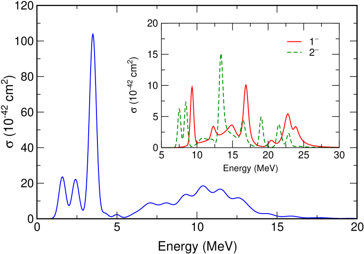
Figure 16: Differential ⁵⁶Fe$(\nu_{e},e^{-}){}^{56}$Co cross section for the KARMEN neutrino spectrum, coming from the decay at rest of the muon, as a function of the excitation energy in ⁵⁶Co. The figure shows the allowed contributions, while the inset gives the contribution of the 1^- and 2^- multipolarities.

In the capture process on nuclei, the electron has to overcome the Q-values of the nuclei and the internal excitation energy of the GT states in the daughter, so the final neutrino energies are noticeably smaller than for capture on free protons. Typical neutrino spectra for a presupernova model are shown in figure 15. In this stage of the collapse the neutrino energies are sufficiently small that they only excite allowed transitions. Consequently neutrino-nucleus cross sections for $pf$-shell nuclei can be determined on the basis of GT distributions determined in the shell model. In the later stage of the collapse, the increased density results also in higher energy electrons ($E_{e}\sim\rho^{1/3}$) which in turn, if captured by protons or nuclei, produce neutrinos with energies larger than 15–20 MeV. For such neutrinos forbidden (mainly $\lambda=1$ dipole and spin-dipole) transitions can significantly contribute to the neutrino-nucleus cross section. Such a situation is shown in figure 16 which shows the differential cross section for the process ⁵⁶Fe$(\nu_{e},e^{-}){}^{56}$Co computed using the Shell-Model for the Gamow-Teller contribution and the CRPA for the forbidden contributions Kolbe et al. (1999a). The calculation adopts a neutrino spectrum corresponding to a muon decaying at rest. The average energy, $\bar{E}_{\nu}\approx 30$ MeV, and momentum transfer, $q\approx 50$ MeV, represent the maximum values for $\nu_{e}$ neutrinos expected during the supernova collapse phase, i.e., the maximum contribution expected from forbidden transitions to the total neutrino-nucleus cross sections. In this particular case the $1^{+}$ multipole (Gamow-Teller at the $q=0$ limit) represents 50% of the cross section. The ⁵⁶Fe$(\nu_{e},e^{-}){}^{56}$Co cross section for neutrinos from muon-decay at rest has been measured by the Karmen collaboration. The measured cross section ($2.56\pm 1.08({\rm stat})\pm 0.43({\rm syst})\times 10^{-40}$ cm²) Zeitnitz (1994) agrees with the result calculated in the shell model (allowed transitions) plus CRPA (forbidden transitions) approach ($2.38\times 10^{-40}$ cm²) Kolbe et al. (1999a).

Although the most important neutrino reactions during collapse are coherent elastic scattering on nuclei and inelastic scattering off electrons, it has been noted Haxton (1988); Bruenn and Haxton (1991) that neutrino-induced reactions on nuclei can happen as well. Using ⁵⁶Fe as a representative nucleus, Bruenn and Haxton concluded that charged-current $(\nu_{e},e^{-})$ reactions do not have an appreciable effect on the evolution of the core during infall, due to the high-threshold for neutrino absorption. Based on shell model calculations of the GT strength distributions, Sampaio et al. (2001) confirmed this finding for other, more relevant nuclei in the core composition. The same authors showed that finite-temperature effects can increase the $(\nu_{e},e^{-})$ cross sections for low neutrino energies drastically Sampaio et al. (2001). But this increase is found to be significantly smaller than the reduction of the cross section caused by Pauli blocking of the final phase space, i.e. due to the increasing electron chemical potential. This environmental effect ensures that neutrino absorption on nuclei is unimportant during the collapse compared with inelastic neutrino-electron scattering.

Figure 17: Inelastic neutrino cross sections for ⁵⁶Fe (left) and ⁵⁹Co (right) as function of initial neutrino energy and for selected temperatures (upper part). Only allowed Gamow-Teller transitions have been considered. Temperatures are in MeV. For $T=0$, the cross section is calculated for the ground state only. At $T>0$, the cross sections have been evaluated for a thermal ensemble of initial states. The corresponding neutrino energy distribution in the final state is shown in the lower part, assuming an initial neutrino energy of $E_{\nu}=7.5$ MeV. Due to threshold effects a significant portion of the neutrinos are upscattered in energy for even-even nuclei.

Bruenn and Haxton (1991) observed that inelastic neutrino scattering off nuclei plays the same important role of equilibrating electron neutrinos with matter during infall as neutrino-electron scattering. The influence of finite temperature on inelastic neutrino-nucleus scattering was studied in Fuller and Meyer (1991), using an independent particle model. While the study in Bruenn and Haxton (1991) was restricted to ⁵⁶Fe, additional cross sections have been calculated for inelastic scattering of neutrinos on other nuclei based on modern shell-model GT strength distributions Sampaio et al. (2002b). Again, for low neutrino energies the cross sections are enhanced at finite temperatures (figure 17). This is caused by the possibility that, at finite temperatures, the initial nucleus can reside in excited states which can be connected with the ground state by sizable GT matrix elements. These states can then be deexcited in inelastic neutrino scattering. Note that in this case the final neutrino energy is larger than the initial (see figure 17) so that the deexcitation occurs additionally with larger phase space. Until neutrino trapping there is little phase space blocking in inelastic neutrino-nucleus scattering. Toivanen et al. (2001) presented the charged- and neutral-current cross sections for neutrino-induced reactions on the iron isotopes ^52-60Fe, using a combination of shell model and RPA approach. Other possible neutrino processes, e.g. nuclear deexcitation by neutrino pair production (13k), have been discussed in Fuller and Meyer (1991), but the estimated rates are probably too small for these processes to be important during the collapse.

Finally we remark that coherent elastic scattering on nuclei scales like $\sim E_{\nu}^{2}$ so that neutrinos with low energies are the last to be trapped. In order to fill this important sink for entropy and energy, processes which affect the production of neutrinos with low energies can be quite relevant for the collapse. Inelastic neutrino scattering on nuclei, including finite temperature effects, is one such process Bruenn and Haxton (1991). The significantly lower energies of the neutrinos generated by electron capture on nuclei than the ones generated by capture on free protons is another reason to implement these processes with appropriate care in collapse simulations.

V.3 Delayed supernova mechanism

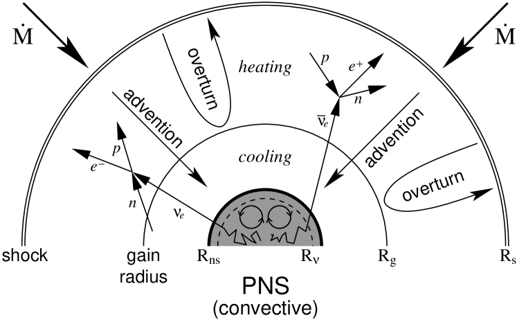
Figure 18: Sketch of the stellar core during the shock revival phase. $R_{\nu}$ is the neutrinosphere radius, from which neutrinos are expected to stream out freely, $R_{ns}$ is the radius of the protoneutron star, $R_{g}$ the gain radius (see text) and $R_{s}$ the radius at which the shock is stalled. The shock expansion is impeded by mass infall at a rate ${\dot{M}}$, but supported by convective energy transport from the region of strongest neutrino heating to the stalled shock. Convection inside the protoneutron star (PNS) as well as correlations in the dense nuclear medium increase the neutrino luminosity (adapted from Janka et al., 2001).

In the delayed supernova mechanism the fate of the explosion is determined by several distinct neutrino processes. When the shock reaches the $\nu_{e}$ neutrinosphere, from which $\nu_{e}$ are expected to stream out freely, electron capture on the shock-heated and shock-dissociated matter increases the $\nu_{e}$ production rate significantly. Additionally neutrinos are produced by the transformation of electron-positron pairs into $\nu\bar{\nu}$ pairs (equation 13j). This process is strongly temperature dependent (e.g. Soyeur and Brown, 1979) and occurs most effectively in the shock-heated regions of the proto-neutron star. Electron-positron pair annihilation and nucleon-nucleon bremsstrahlung (equation 13f) generate pairs of all three neutrino flavors with the same probability and thus are the main mechanisms for the production of $\nu_{\mu}$, $\nu_{\tau}$ neutrinos and antineutrinos Raffelt (2001); Hanhart et al. (2001); Stoica and Horvath (2002); Hannestad and Raffelt (1998); Hannestad (2001); Thompson and Burrows (2001); Thompson et al. (2000). The emitted $\nu_{e}$ and $\bar{\nu}_{e}$ neutrinos, however, can be absorbed again by the free nucleons behind the shock. Due to the temperature and density dependences of the neutrino processes involved, neutrino emission wins over neutrino absorption in a region inside a certain radius (the gain radius), while outside the gain radius matter is heated by neutrino interactions that are dominated by absorption of electron neutrinos and antineutrinos on free nucleons which have been previously liberated by dissociation due to the shock (see figure 18). As a net effect, neutrinos transport energy across the gain radius to the layers behind the shock. Due to the smaller abundances, neutrino-induced reactions on finite nuclei are expected to contribute only modestly to the shock revival. It has been also suggested that the shock revival is supported by ‘preheating’ Haxton (1988). In this scenario the electron neutrinos, which have been trapped during the final collapse phase and are liberated in a very short burst (with luminosities of a few $10^{53}$ erg s^-1 lasting for about 10 ms), can partly dissociate the matter (e.g. iron and silicon isotopes) prior to the shock arrival. As reliable neutrino-induced cross sections on nuclei have not been available until recently, the neutrino-nucleus reactions have not been included in collapse and post-bounce simulations.

To describe the important neutrino-nucleon processes, most core collapse simulations use the same lowest order cross section for both neutrinos and antineutrinos Bruenn (1985); Horowitz (2002), i.e., they neglect terms of order $E_{\nu}/M$, where $E_{\nu}$ is the neutrino energy and $M$ the nucleon mass. The most important corrections to the cross section at this order are the nucleon recoil and the weak magnetism related to the form factor $F_{2}$ in Eq. (4a) Horowitz (2002). The recoil correction is the same for neutrinos and antineutrinos and decreases the cross sections. However, the weak magnetism corrects the cross sections via its parity-violating interference with the dominant axial-vector component. As the interference is constructive for neutrinos and destructive for antineutrinos, inclusion of the weak magnetism correction increases the neutrino cross section, while it decreases the $\bar{\nu}$-nucleon cross sections. It is then expected that corrections up to order $E_{\nu}/M$ decrease the antineutrino cross section noticeably (by about $25\%$ for 40 MeV antineutrinos), while the $\nu$-nucleon cross sections are only affected by a few percents for $E_{\nu}\leq 100$ MeV Horowitz (2002).

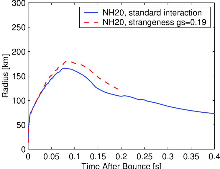
Figure 19: Shock trajectories of a 20 $M_{\odot}$ star, calculated with (dashed) and without (solid) an isoscalar strange axialform factor in the neutrino-nucleon elastic cross sections (courtesy of M. Liebendörfer).

Neutral-current processes are sensitive to possible strange quark contributions in the nucleon which would give rise to an isoscalar piece $g_{A}^{s}$ in the axial-vector form factor besides the standard isovector form factor $g_{A}\bm{\tau}$ Jaffe and Manohar (1990); Beise and McKeown (1991). The current knowledge on $g_{A}^{s}$ comes from a $\nu p$ elastic scattering experiment performed at Brookhaven yielding $g_{A}^{s}=-0.15\pm 0.08$ Ahrens et al. (1987), but is considered rather uncertain Garvey et al. (1993b). With $g_{A}=1.26$ and assuming axial-vector dominance, i.e. the cross section scales like $\sigma\sim|g_{A}\bm{\tau}-g_{A}^{s}|^{2}$, a non-vanishing strange axial-vector form factor would reduce the elastic scattering cross section on neutrons and increase the $\nu p$ elastic cross section Garvey et al. (1992); Garvey et al. (1993a); Horowitz (2002). As the matter behind the shock is neutron-rich, the net effect will be a reduction of the neutrino-nucleon elastic cross section. This increases the energy transfer to the stalled shock, however, a simulation has shown that this increase is not strong enough for a successful shock revival (Liebendörfer et al., 2002, see figure 19).

The physics involved in the attempt to revive the shock by neutrino heating is exhaustively reviewed by Janka et al. (2001) (see also Burrows and Goshy, 1993). These authors show that the fate of the stalled shock does not only depend on the neutrino heating above the gain radius, but is also influenced by the energy loss in the cooling region below the gain radius (see also Bethe and Wilson, 1985). Janka (2001) also demonstrates the existence of a critical value for the neutrino luminosity from the neutron star needed to revive the shock. This critical luminosity depends on the neutron star mass and radius and on the mass infall to the shock. One expects that the shock expansion is eased for high mass infall rates, which increase the matter pile-up on the neutron star and push the shock outwards, and for high $\nu_{e}$ and $\bar{\nu}_{e}$ luminosities from the neutron star, which lead to an enhancement of neutrino absorption relative to neutrino emission in the gain region.

The explosion depends crucially on the effectiveness by which energy is transported by neutrinos to the region where the shock has stalled. As stressed before, one-dimensional models including sophisticated neutrino transport (e.g. Rampp and Janka, 2000; Liebendörfer et al., 2001) fail to explode. However, the neutrino energy transport is very sensitive to: i) the effect of nucleon-nucleon correlations on the neutrino opacities in dense matter and ii) convection both in the neutrino-heated region and in the proto-neutron star Janka et al. (2001).

In his pioneering work, Sawyer (1989) calculated the neutrino mean free path, or equivalently the neutrino opacity, in uniform nuclear matter and showed that effects due to strong interaction between nucleons are important. The same conclusion has been reached by Raffelt et al. (1996) who demonstrated that the average neutrino-nucleon cross section in the medium is reduced due to spin fluctuations induced by the spin-dependent interaction among nucleons. (For earlier calculations of the neutrino mean free path in uniform nuclear matter, see Sawyer, 1975; Friman and Maxwell, 1979; Iwamoto and Pethick, 1982). Sawyer (1989) exploited the relation between the equation of state (EOS) of the matter and the long-wavelength excitations of the system to calculate the weak interaction rates. However, consistency between the EOS and the neutrino opacities are more difficult to achieve for large energy ($q_{0}$) and momentum ($q$) transfer of the neutrinos. Here, particle-hole and particle-particle interactions are examples of effects which might influence the EOS and the neutrino opacities. For the following discussion it is quite illuminating to realize the similarity of the neutrino-induced excitations of nuclear matter with the physics of multipole giant resonances in finite nuclei.

For muon and tau neutrinos, neutral current reactions are the only source of opacities. Here, the energy and momentum transfer is limited by the matter temperature alone. For electron neutrinos the mean free path is dominated by charged-current reactions, for which the energy transfer is typically of the order of the difference between neutron and proton chemical potentials. During the early deleptonization epoch of the proto-neutron star the typical neutron momenta are large ($\sim 100$–200 MeV) and the mismatch of proton, neutron and electron Fermi momenta can be overcome by the neutrino momenta. This is not longer possible in later stages when the neutrino energies are of order $k_{b}T$; then momentum conservation restricts the available phase space for the absorption reaction. Pauli blocking of the lepton in the final state increases the mean free path for charged-current and neutral-current reactions.

We note an important and quite general consequence of the fact that muon and tau neutrinos react with the proto-neutron star matter only by neutral-current reactions: The four neutrino types have similar spectra. Due to universality, $\nu_{\mu}$, $\nu_{\tau}$ and $\bar{\nu}_{\mu}$, $\bar{\nu}_{\tau}$ have identical spectra. It is usually even assumed that neutrinos and antineutrinos have the same spectra (one therefore refers to the 4 neutrino types unifyingly as $\nu_{x}$ neutrinos) exploiting axial-vector dominance in the neutrino cross sections. However, the interference of the axial-vector and the weak magnetism components makes the $\bar{\nu}_{x}$ spectra slightly hotter than the $\nu_{x}$ spectra. The $\nu_{x}$ neutrinos decouple deepest in the star, i.e., at a higher temperature, than electron neutrinos and antineutrinos, and hence have higher energies. As the matter in the proto-neutron star is neutron-rich, electron neutrinos, which are absorbed by neutrons, decouple at a larger radius than their antiparticles, which interact with protons by charged-current reactions. As a consequence decoupled electron neutrinos have, on average, smaller energies than electron antineutrinos. Calculated supernova neutrino spectra can be found in Janka and Hillebrandt (1989); Yamada et al. (1999), which yield the average energies of the various supernova neutrinos approximately as: $\langle E_{\nu_{e}}\rangle=11$ MeV, $\langle E_{\bar{\nu}_{e}}\rangle=16$ MeV, and $\langle E_{\nu_{x}}\rangle=25$ MeV. Burrows et al. (2000) find the same hierarchy, but somewhat smaller average neutrino energies.

For a much deeper and detailed description of the neutrino mean free paths in dense matter the reader is refered to Reddy et al. (1999); Prakash et al. (2001) and the earlier work Reddy et al. (1998); Burrows and Sawyer (1998, 1999). We will here only briefly summarize the essence of the work presented in these references.

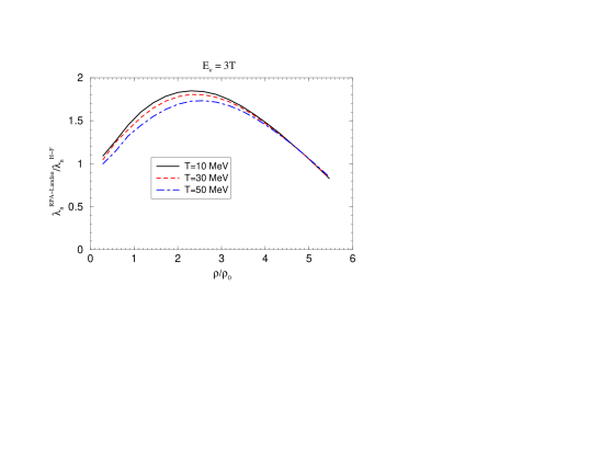
Figure 20: Ratio of neutrino mean free paths in neutron matter calculated in RPA and Hartree-Fock approaches at various temperatures Margueron et al. (2002). The interaction is the Gogny force D1P. The neutrino energy is taken as $E_{\nu}=3T$.

Collapse simulations describe neutrino opacities typically on the mean-field level or even by a nucleon gas. Then an analytical expression can be derived for the vector and axial-vector response of the medium which in turn determines the charged- and neutral-current cross sections. Effects due to the strong interaction between nucleons are considered by a medium-dependent effective mass in the dispersion relation. Like in finite nuclei, collective excitations in nuclear matter arise due to nucleon-nucleon correlations beyond the mean-field approximation. As it is believed that single-pair excitations dominate over multi-pair excitations for the kinematics of interest to neutrino scattering and absorption, it appears to be sufficient to determine the vector and axial-vector response, in a first step, within the Random Phase Approximation (RPA). Assuming that the interaction is short-ranged compared to the wavelength of the excitations, it is justified to retain only s-wave components in the interaction which in turn can be related to Fermi-liquid parameters. It is found that the repulsive nature of the parameter $G_{0}^{\prime}$, which is related to the isovector spin-flip or giant Gamow-Teller resonances in nuclei, induces a collective state in the region $\omega/q\sim v_{F}$ ($v_{F}$ is the Fermi velocity), while the cross section is reduced at smaller energies. However, these smaller energies are important for the neutrino mean free path at nuclear matter densities ($\rho_{0}$) or smaller densities. Assuming a typical neutrino energy $E_{\nu}\approx 3T$ (corresponding to a Fermi-Dirac distribution with temperature $T$ and zero chemical potential) RPA correlations increase the neutral-current neutrino mean-free path (see figure 20) at low temperatures and for $\rho=\rho_{0}$, compared with the mean-field result. An enhancement due to RPA correlations is also found for neutrino absorption mean-free paths for neutrino-trapped matter. Like in the case of neutrino-induced reactions on finite nuclei (see above), finite-temperature effects allow that nuclear excitation energy is transferred to the neutrino in inelastic scattering processes. This contributes to the cooling of the nuclear matter and increases the neutrino energy in the final state.

Neutrino heating is maximal in the layer just above the gain radius. The energy transport from this region to the shock, which is stalled further out, can be supported by convective overturn and might lead to successful explosions, as has been demonstrated in several simulations with two-dimensional hydrodynamics treatment of the region between the gain radius and the shock Herant et al. (1994); Burrows et al. (1995); Janka and Müller (1996). The effect of convection is twofold Janka et al. (2001): At first, heated matter is transported outwards to cooler regions where the energy loss due to neutrino emission is reduced (the neutrino production rate for electron and positron captures on nucleons depends strongly on temperature). Second, cooler matter is brought down closer to the gain radius where the neutrino fluxes are larger and hence the heating is more effective. While this picture is certainly appealing, it is not yet clear whether multi-dimensional simulations will indeed lead to explosions as the two-dimensional studies did not include state-of-the-art Boltzmann neutrino transport, but treated neutrino transport in an approximate manner. In fact, in a simulation with an improved treatment of neutrino transport the convective overturn was found not to be strong enough to revive the stalled shock Mezzacappa et al. (1998).

The shock revival can also be supported by convection occuring inside the protoneutron star where it is mainly driven by the negative lepton gradient which is established by the rapid loss of leptons in the region around the neutrinosphere Burrows (1987); Keil et al. (1996). By this mode, lepton-rich matter will be transported from inside the protoneutron star to the neutrinosphere which increases the neutrino luminosity and thus is expected to help the explosion. The simulation of protoneutron star convection is complicated by the fact that neutrinos and matter are strongly coupled. In fact, two-dimensional simulations found that neutrino transport can equilibrate otherwise convective fluid elements Mezzacappa et al. (1998). Such a damping is possible in regions where neutrinos are still strongly coupled to matter, but neutrino opacities are not too high to make neutrino transport insufficient. In the model of Keil et al. (1996) the convective mixing occurs very deep inside the core where the neutrino opacities are high; no damping of the convection by neutrinos is then found.

Wilson and Mayle attempted to simulate convection in their spherical model by introducing neutron-fingers and found successful explosions Wilson and Mayle (1993). This idea is based on the assumption that energy transport (by three neutrino flavors) is more efficient than lepton number transport (only by electron neutrinos). However, this assumption is under debate Bruenn and Dineva (1996).

VI Nucleosynthesis beyond iron

While the elements lighter than mass number $A\sim 60$ are made by charged-particle fusion reactions, the heavier nuclei are made by neutron captures, which have to compete with $\beta$ decays. Already Burbidge et al. (1957); Cameron (1957) realized that two distinct processes are required to make the heavier elements. This is the slow neutron-capture process (s-process), for which the $\beta$ lifetimes $\tau_{\beta}$ are shorter than the competing neutron capture times $\tau_{n}$. This requirement ensures that the s-process runs through nuclei in the valley of stability. The rapid neutron-capture process (r-process) requires $\tau_{n}\ll\tau_{\beta}$. This is achieved in extremely neutron-rich environment, as $\tau_{n}$ is inversely proportional to the neutron density of the environment. The r-process runs through very neutron-rich, unstable nuclei, which are far-off stability and whose physical properties are often experimentally unknown.

Weak-interaction processes play interesting, but different roles in these processes. The half-lives of the $\beta$-unstable nuclei along the s-process path are usually known with good precision. However, the nuclear half-life in the stellar environment can change due to the thermal population of excited states in the parent nucleus. This is particularly interesting if the effective lifetime is then comparable to $\tau_{n}$, leading to branchings in the s-process path, from which the temperature and neutron density of the environment can be determined. Several recent examples are discussed in the next subsection. For the r-process, $\beta$-decays are probably even more crucial. They regulate the flow to larger charge numbers and determine the resulting abundance pattern and duration of the process. Except for a few key nuclei, $\beta$-decays of r-process nuclei have to be modelled theoretically; we will briefly summarize the recent progress below. Although the r-process site is not yet fully determined, it is conceivable that it occurs in the presence of extreme neutrino fluxes. As we will discuss, neutrino-nucleus reactions can have interesting effects during and after the r-process, perhaps allowing for clues to ultimately identify the r-process site.

VI.1 S-process

The analysis of the solar abundances have indicated that two components of the s-process have contributed to the synthesis of elements heavier than $A\sim 60$. The weak component produces the elements with $A\lesssim 90$. Its site is related with helium core burning of CNO material in more massive stars Couch et al. (1974); Käppeler et al. (1994). The main component, which is responsible for the heavier s-process nuclides up to Pb and Bi, is associated with helium flashes occurring during shell burning in low-mass (asymptotic giant branch) stars Busso et al. (1999). The ²²Ne($\alpha,n)^{25}$Mg and ¹³C($\alpha,n)^{16}$O reactions are believed to be the supplier of neutrons for the weak and main components, respectively. The s-process abundances $N_{s}$ are found to be inversely proportional to the respective (temperature averaged) neutron capture cross sections $\langle\sigma\rangle$, as expected for a steady-flow picture Burbidge et al. (1957), which, however, breaks down for the extemely small cross sections at the magic neutron numbers. As a consequence, the product $N_{s}\cdot\langle\sigma\rangle$ exhibits almost constant plateaus between the magic neutron numbers, separated by pronounced steps, (e.g. Käppeler, 1999).

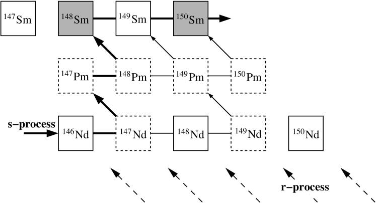
Figure 21: The s-process reaction path in the Nd-Pm-Sm region with the branchings at $A=147$, 148, and 149. Note that ¹⁴⁸Sm and ¹⁵⁰Sm are shielded against r-process $\beta$-decays (adapted from Käppeler, 1999).

The neutron density of the stellar environment during the main s-process component can be determined from branching points occuring, for example, in the $A=147$–149 mass region (see figure 21). Here the relative abundances of the two s-process-only isotopes ¹⁴⁸Sm and ¹⁵⁰Sm ($Z=62$), which are shielded against r-process contributions by the two stable Nd ($Z=60$) isotopes ¹⁴⁸Nd and ¹⁵⁰Nd, is strongly affected by branchings occuring at ¹⁴⁷Nd and, more importantly, at ¹⁴⁸Pm and at ¹⁴⁷Pm. As the neutron captures on these branching nuclei will bypass ¹⁴⁸Sm in the flow pattern, the ¹⁵⁰Sm $N_{s}\langle\sigma\rangle$ value will be larger for this nucleus than for ¹⁴⁸Sm. Furthermore, the neutron capture rate $\lambda_{n}$ is proportional to the neutron density $N_{n}$. Thus, $N_{n}$ can be determined from the relative ¹⁵⁰Sm/¹⁴⁸Sm abundances, resulting in $N_{n}=(4.1\pm 0.6)\times 10^{8}$ cm^-3 Toukan et al. (1995). A similar analysis for the weak s-process component yields neutron densities of order $(0.5\text{--}1.3)\times 10^{8}$ cm^-3 Walter et al. (1986a, b). We stress that a 10% determination of the neutron density requires the knowledge of the involved neutron capture cross sections with about 1% accuracy Käppeler et al. (1998), which has yet not been achieved for unstable nuclei. Improvements are expected from new time-of-flight facilities like LANSCE at Los Alamos or NTOF at CERN.

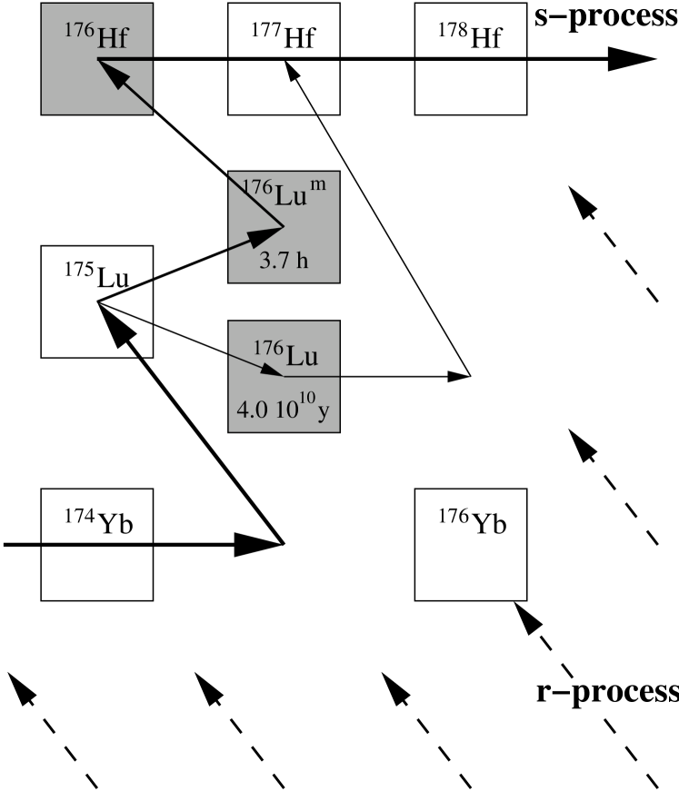
Figure 22: The s-process neutron capture path in the Yb-Lu-Hf region (solid lines). For ¹⁷⁶Lu the ground state and isomer are shown separately. Note that ¹⁷⁶Lu and ¹⁷⁶Hf are shielded against r-process $\beta$-decays (adapted from Doll et al., 1999).

Figure 23: The figure shows an schematic energy-level diagram of ¹⁸⁰Ta and its daughters illustrating the possibility for thermally enhanced decay of ¹⁸⁰Ta^m in the stellar environment of the s-process. The inset shows the photon density at s-process temperature (adapted from Belic et al., 1999).

The temperature of the s-process environment can be ‘measured’, if the $\beta$ half-life of a branching point nucleus is very sensitive to the thermal population of excited nuclear levels. A prominent example is ¹⁷⁶Lu Beer et al. (1981). For mass number $A=176$, the $\beta$-decays from the r-process terminate at ¹⁷⁶Yb ($Z=70$), making ¹⁷⁶Hf ($Z=72$) and ¹⁷⁶Lu ($Z=71$) s-only nuclides (see figure 22). Besides the long-lived ground state ($t_{1/2}=4.00(22)\times 10^{10}$ y), ¹⁷⁶Lu has an isomeric state at an excitation energy of 123 keV ($t_{1/2}=3.664(19)$ h). Both states can be populated by ¹⁷⁵Lu$(n,\gamma)$ with known partial cross sections. At ¹⁷⁶Lu, the s-process matter flow is determined by the competition of neutron capture on the ground state and $\beta$-decay of the isomer. But importantly, the ground and isomeric states couple in the stellar photon bath via the excitation of an intermediate state at 838 keV (figure 23 shows a similar process taking place in ¹⁸⁰Ta), leading to a matter flow from the isomer to the ground state, which is very temperature-dependent. A recent analysis of the ¹⁷⁶Lu s-process branching yields an environment temperature of $T=(2.5\text{--}3.5)\times 10^{8}$ K Doll et al. (1999).

Similar finite-temperature effects play also an important role in the s-process production of ¹⁸⁰Ta. This is the rarest isotope (0.012%) of nature’s rarest element. It only exists in a long-lived isomer ($J^{\pi}=9^{-}$) at an excitation energy of 75.3 keV and with a half-life of $t_{1/2}\geq 1.2\times 10^{15}$ y. The $1^{+}$ ground state decays with a half-life of 8.152(6) h, mainly by electron capture to ¹⁸⁰Hf. While potential s-process production paths of the ¹⁸⁰Ta isomer have been pointed out, the survival of this state in a finite-temperature environment has long been questionable. While a direct electromagnetic decay to the ground state is strongly suppressed due to angular momentum mismatch, the isomer can decay via thermal population of intermediate states with branchings to the ground state (see figure 23). By measuring the relevant electromagnetic coupling strength, the temperature-dependent half-life, and thus the ¹⁸⁰Ta survival rate, has been determined by Belic et al. (1999) under s-process conditions as $t_{1/2}\lesssim 1$ y, i.e. more than 15 orders of magnitude smaller than the half-life of the isomer! Accompanied by progress in stellar modeling of the convective modes during the main s-process component (which brings freshly produced ¹⁸⁰Ta to cooler zones, where it can survive more easily, on timescales of days) it appears now likely that ¹⁸⁰Ta is partly made within s-process nucleosynthesis Wisshak et al. (2001). The p-process Rayet et al. (1995) and neutrino nucleosynthesis Woosley et al. (1990) have been proposed as alternative sites for the ¹⁸⁰Ta production.

The two neighboring isotopes ¹⁸⁶Os and ¹⁸⁷Os are s-process only nuclides, shielded against the r-process by ¹⁸⁶W and ¹⁸⁷Rh. The nucleus ¹⁸⁷Rh has a half-life of 42 Gy which is comparable with the age of the universe. As the ¹⁸⁷Rh decay has contributed to the observed ¹⁸⁷Os abundance, the Os/Rh abundance ratio can serve as a sensitive clock for the age of the universe, once the s-process component is subtracted from the ¹⁸⁷Os abundance Clayton (1964). To determine the latter precise measurements of the neutron capture cross sections on ¹⁸⁶Os and ¹⁸⁷Os are required, which are in progress at CERN’s NTOF facility. A potential complication arises from the fact that ¹⁸⁷Os has a low-lying state at 9.8 keV which is populated equally with the ground state at s-process temperatures. The respective neutron capture cross sections on the excited state can be indirectly determined from (n,n’) measurements. Furthermore one has to consider that the half-life of ¹⁸⁷Rh is strongly temperature-dependent: If stripped of its electrons, the half-life is reduced by 9 orders of magnitude to $t_{1/2}=32.9\pm 2$ y as measured at the GSI storage ring Bosch et al. (1996). However, the GSI data can be translated into a $\log ft$ value from which the ¹⁸⁷Rh half-life can be deduced for every ionization state.

The decay of totally ionized ¹⁸⁷Rh is an example for a bound state $\beta$-decay, i.e., the decay of bare ¹⁸⁷Rh⁷⁵⁺ to continuum states of ¹⁸⁷Os⁷⁶⁺ is energetically forbidden, but it is possible if the decay electron is captured in the K-shell ($Q_{\beta}$=73 keV) or in the L-shell ($Q_{\beta}$=9.1 keV) Johnson and Soff (1985). We note that the decay of neutral ¹⁸⁷Rh is energetically allowed for a first-forbidden transition to the ¹⁸⁷Os ground state; the long half-life results from the small matrix element and $Q_{\beta}$ value related to this transition. Another example of a bound state $\beta$-decay with importance for the s-process occurs for ¹⁶³Dy. This nucleus is stable as a neutral atom, but, if fully ionized, can decay to ¹⁶³Ho with a half-life of $47^{+5}_{-4}$ d; the measurement of this half-life at the GSI storage ring was the first observation of bound state $\beta$-decay Jung et al. (1992). The consideration of the ¹⁶³Dy decay at s-process conditions has been found to be essential to explain the abundance of the s-process only nuclide ¹⁶⁴Er, which is produced by neutron capture on ¹⁶³Ho, the daughter of the bound state $\beta$-decay of ¹⁶³Dy, and the subsequent $\beta$-decay of ¹⁶⁴Ho to ¹⁶⁴Er.

VI.2 R-process

Phenomenological parameter studies indicate that the r-process occurs at temperatures around $T\sim 100$ keV and at extreme neutron fluxes (neutron number densities $n>10^{20}$ cm^-3) (e.g. Cowan et al., 1991). It has also been demonstrated that not all r-process nuclides can be made simultaneously at the same astrophysical conditions (constant temperature, neutron density), i.e. the r-process is a dynamical process with changing (different) conditions and paths Kratz et al. (1993). In a good approximation, the neutron captures proceed in $(n,\gamma)\rightleftarrows(\gamma,n)$ equilibrium, fixing the reaction paths at rather low neutron separation energies of $S_{n}\sim 2$–3 MeV Cowan et al. (1991), implying paths through very neutron-rich nuclei in the nuclear chart as is shown in figure 24. While the general picture of the r-process appears to be well accepted, its astrophysical site is still open. The extreme neutron fluxes point to explosive scenarios and, in fact, the neutrino-driven wind above the nascent neutron star in a core-collapse supernova is the currently favored model Witti et al. (1994a, b); Woosley et al. (1994). But also shock-processed helium shells in type II supernovae Truran et al. (2001) and neutron star mergers Freiburghaus et al. (1999b); Rosswog et al. (2000) are investigated as possible r-process sites. Recent meteoritic clues Wasserburg et al. (1996); Qian et al. (1998) as well as observations of r-process abundances in low-metallicity stars Sneden et al. (2000) point to more than one distinct site for the solar r-process nuclides.

In an important astronomical observation Cayrel et al. (2001) have recently detected the r-process nuclides thorium and uranium in an old galactical halo star. As these two nuclei have halflives, which are comparable to the expected age of the universe, their measured abundance ratio serves as a sensitive clock to determine a lower limit to this age, provided their initial r-process production abundance ratio can be calculated with sufficient accuracy. Cayrel et al. (2001) have used their observed ²³⁸U/²³²Th abundance ratio from the star CS31082-001 and the r-process model predictions from Cowan et al. (1999); Goriely and Clerbaux (1999) to deduce a value of $12.5\pm 3.3$ Gyr for the age of the star. Recently, a refined analysis of the CS31082-001 spectra has led to a significant improvement in the derived abundances which provides now an age estimate of $14.0\pm 2.4$ Gyr Hill et al. (2002). The effect of different nuclear physics input on the r-process production of U and Th have been studied by Goriely and Arnould (2001) and by Schatz et al. (2002)

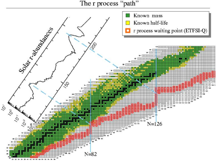
Figure 24: The r-process occurs under dynamically changing astrophysically conditions which affect the reaction pathway. The figure shows the range of r-process paths, defined by their waiting point nuclei. After decay to stability the abundance of the r-process progenitors produce the observed solar r-process abundance distribution. The r-process paths run generally through neutronrich nuclei with experimentally unknown masses and halflives. In this calculation a mass formula based on the Extended Thomas Fermi model with Strutinski Integral (ETFSI) and special treatment of shell quenching (see text) has been adopted. (courtesy of Karl-Ludwig Kratz and Hendrik Schatz).

As relevant nuclear input, r-process simulations require neutron separation energies (i.e. masses), half-lives and neutron capture cross sections of the very neutron-rich nuclei on the various dynamical r-process paths. As currently only few experimental data are known for r-process nuclei, these quantities have to be modelled. Traditionally this has been done by global models which, by fitting a certain set of parameters to known experimental data, are then being used to predict the properties of all nuclei in the nuclear landscape. Arguably the most important input to r-process simulations are neutron separation energies as they determine, for given temperature and neutron density of the astrophysical environment, the r-process paths. The most commonly used mass tabulations are based on the microscopic-macroscopic finite-range droplet model (FRDM) approach Möller et al. (1997) or the Extended Thomas-Fermi model with Strutinski Integral (ETFSI) approach Aboussir et al. (1995). In more recent developments mass tabulations have been developed adopting parametrizations inspired by shell model results Duflo and Zuker (1995) or calculated on the basis of nuclear many-body theories like the Hartree-Fock model with a BCS treatment of pairing Goriely et al. (2001). Special attention has been paid recently also to the ‘shell quenching’, i.e. the observations made in HFB calculations that the shell gap at magic neutron numbers is less pronounced in very neutron-rich nuclei than in nuclei close to stability Dobaczewski et al. (1994). Such a vanishing of the shell gap has been experimentally verified for the magic neutron number $N=20$ Guillemaud-Mueller et al. (1984); Motobayashi et al. (1995). The confirmation of the predicted quenching at the $N=82$ shell closure is the aim of considerable current experimental activities Kratz et al. (2000). Recent theoretical studies on this topic are reported in Sharma and Farhan (2001, 2002). The potential importance of shell quenching for the r-process rests on the observation Chen et al. (1995); Pfeiffer et al. (1997) that it can correct the strong trough just below the r-process peaks in the calculated r-process abundances encountered with conventional mass models. Neutron capture cross sections become important, if the r-process flow drops out of $(n,\gamma)\rightleftarrows(\gamma,n)$ equilibrium, which happens close to freeze-out when the neutron source ceases. They can also be relevant for nuclides with small abundances for which no flow equilibrium is built up Surman et al. (1997); Surman and Engel (2001). In the following we will summarize recent progress in calculating half-lives for nuclei on the r-process paths.

VI.2.1 Half-Lives

The nuclear half-lives determine the relative r-process abundances. In a simple $\beta$-flow equilibrium picture the elemental abundance is proportional to the half-life, with some corrections for $\beta$-delayed neutron emission Kratz et al. (1988). As r-process half-lives are longest for the magic nuclei, these waiting point nuclei determine the minimal r-process duration time; i.e. the time needed to build up the r-process peak around $A\sim 200$ via matter-flow from the seed nucleus. We note, however, that this time depends also crucially on the r-process path.

Pioneering experiments to measure half-lives of neutron-rich isotopes near the r-process path succeeded in determining the half-lives of two $N=50$ (⁸⁰Zn, ⁷⁹Cu) and two $N=82$ (¹²⁹Ag, ¹³⁰Cd) waiting point nuclei Gill et al. (1986); Kratz et al. (1986); Pfeiffer et al. (2001). Pfeiffer et al. (2001) reviewed the experimental information on r-process nuclei. These data play crucial roles in constraining and testing nuclear models, which are still necessary to predict the bulk of half-lives required in r-process simulations. It is generally assumed that the half-lives are determined by allowed Gamow-Teller (GT) transitions. The calculations of $\beta$-decays require usually two ingredients: the GT strength distribution in the daughter nucleus and the relative energy scale between parent and daughter, i.e. their mass difference. However, the $\beta$ decays only probe the weak low-energy tail of the GT distributions. Only a few percent of the $3(N-Z)$ Ikeda sum rule Ikeda et al. (1963) lie within the $Q_{\beta}$ window (i.e. at energies accessible in $\beta$-decay), the rest being located in the region of the Gamow-Teller resonance at higher excitation energies. Due to the strong $E^{5}$ energy dependence of the phase space $\beta$-decay rates are very sensitive to the correct description of the detailed low-energy GT distribution and its relative energy scale to the parent nucleus. This explains why different calculations of the $\beta$-decay half-lives present large deviations among them.

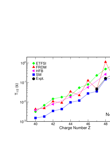
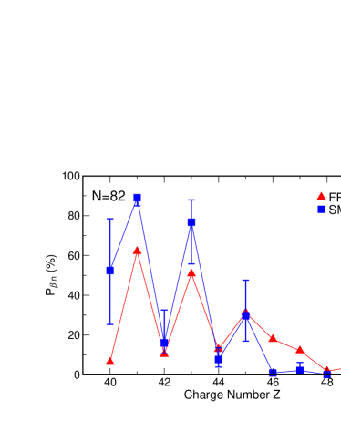
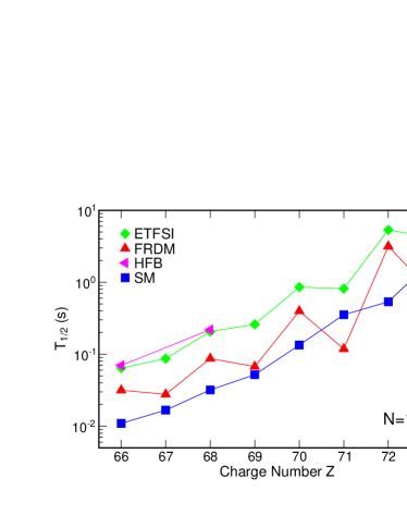
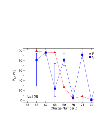
Figure 25: The left panels show the half-lives of the r-process waiting point nuclei with neutron numbers $N=82$ and 126, obtained within different theoretical models. In the case of $N=82$ the half-lives of ¹³¹In, ¹³⁰Cd and ¹²⁹Ag are experimentally known Pfeiffer et al. (2001). The right panels compare the beta-delayed neutron emission probabilities for the $N=82$ (upper) and $N=126$ (lower) waiting-point nuclei as calculated in two different models. For the shell-model (SM) probabilities the error bars indicate the sensitivity of the calculations to a change of $\pm 0.5$ MeV in the neutron separation energies.

Because of the huge number of nuclei relevant for the r-process, the estimates of the half-lives are so far based on a combination of global mass models and the quasiparticle random phase approximation (QRPA), the latter to calculate the GT matrix elements. Examples of these models are the FRDM/QRPA Möller et al. (1997) and the ETFSI/QRPA Borzov and Goriely (2000). Recently, calculations based on the self-consistent Hartree-Fock-Bogoliubov plus QRPA model became available for r-process waiting point nuclei with magic neutron numbers $N=50$, 82 and 126 Engel et al. (1999). The presence of a closed neutron shell has allowed also for the study of these nuclei by shell-model calculations Martínez-Pinedo and Langanke (1999); Martínez-Pinedo (2001), which is the method of choice to determine the $\beta$-decay matrix elements. However an adequate calculation of the nuclear masses for heavy nuclei is yet prohibitive in the shell model. In Martínez-Pinedo and Langanke (1999), and Martínez-Pinedo (2001) the masses were adopted from the global model of Duflo and Zuker (1995). Figure 25 compares the half-lives predicted by the different approaches. For $N=82$, the half-lives of ¹³¹In, ¹³⁰Cd and ¹²⁹Ag are known experimentally Kratz et al. (1986); Pfeiffer et al. (2001). The comparison of the predictions of the different models with the few experimental r-process benchmarks reveals some of their insufficiencies. For example, the FRDM/QRPA half-lives show a significant odd-even staggering which is not present in the data, while the ETFSI/QRPA half-lives appear globally too long. The HFB/QRPA and SM approaches obtain half-lives in reasonable agreement with the data and predict shorter half-lives for the unmeasured waiting point nuclei with $N=82$ than the global FRDM/QRPA and ETFSI/QRPA approaches. For $N=126$ there is no experimental information so the different models remain untested. While HFB calculations for the half-lives of all the r-process nuclei are conceivable, similar calculations within the shell-model approach are still not feasible due to computer memory limitations.

While the $Q_{\beta}$ value for the decay of neutron-rich r-process nuclei is large, the neutron separation energies are small. Hence $\beta$ decay can lead to final states above neutron threshold and is accompanied by neutron emission. If the r-process proceeds by an $(n,\gamma)\rightleftarrows(\gamma,n)$ equilibrium the $\beta$-delayed neutron emission probabilities, $P_{\beta,n}$, only play a role at the end of the r-process when the neutron source has ceased and the produced nuclei decay to stability. The calculated $P_{\beta,n}$ values are very sensitive to both the low-energy GT distribution and the neutron threshold energies. No model describes currently both quantities simultaneously with sufficient accuracy. Figure 25 compares the $P_{\beta,n}$ computed in the FRDM/QRPA and SM approaches for $N=82$ and 126. The predictions between different models can be quite different in experimentally non-determined mass regions. For the SM approach the error bars indicate the sensitivity of the computed $P_{\beta,n}$ values to a change of $\pm 0.5$ MeV in the neutron separation energies of the daughter nucleus; the effect can be large.

It has been pointed out that first-forbidden transitions might have important contributions in some nuclei close to magic numbers Blomqvist et al. (1983); Homma et al. (1996); Korgul et al. (2001). A systematic inclusion of first-forbidden transitions in the calculation of r-process beta-decay half-lives in any of the many-body methods used to describe the GT contributions has not been done. However, a first attempt towards this goal Möller et al. (2002) has combined first-forbidden transitions estimated in the Gross Theory Takahashi et al. (1973) with GT results taken from QRPA calculations. No significant changes compared to r-process studies, which consider only the GT contributions to the halflives, have been observed Kratz (2002).

The presence of low-lying isomeric states in r-process nuclei might change the effective half-lives in the stellar environment. Currently no estimates of these effect exists except for odd-A nuclei with $N=82$. Here shell-model calculations predict half-lives for the isomeric states very similar to the ground state half-lives Martínez-Pinedo and Langanke (1999). The halflives of the isomeric state in ¹²⁹Ag has also been estimated within the QRPA approach and by a second shell model calculation finding values about a factor of 2 larger than the ¹²⁹Ag ground state half-life Kratz (2001). This reference also reports about the first attempt to measure the half-life of the isomeric state.

For heavy nuclei ($Z\geq 84$) some final states populated by $\beta$-decay in the daughter nucleus can also decay by fission Cowan et al. (1991). The relevant beta-delayed fission probabilities depend sensitively on the modelling of the fission barriers Howard and Möller (1980); Mamdouh et al. (2001).

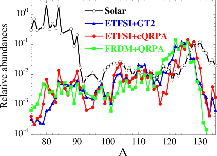
Figure 26: Abundances of r-process nuclides calculated in a dynamical r-process model and for different global sets of $\beta$-decay half-lives. In the dynamical r-process the matter flow timescale competes with the nuclear timescale, set by the $\beta$-decay half-lives. As a consequence the magic neutron numbers (here $N=82$) are reached at different astrophysical conditions and hence at different proton numbers, which is reflected in the shifts of the abundance peaks (from Borzov and Goriely, 2000).

Borzov and Goriely have studied the influence of the $\beta$ half-lives on the r-process abundances within two distinct scenarios: the canonical r-process picture with a exposure of the seed nucleus ⁵⁶Fe by a constant neutron density and temperature for a fixed duration time (2.4 s) and the neutrino-driven wind model. In the canonical model the location of the r-process abundance peaks depends on the masses, but not on the $\beta$ half-lives, which act only as bottlenecks for the matter-flow to more massive nuclei. In the dynamical neutrino-driven wind model the half-lives affect the abundance distribution. This comes about as at later times in this model the environmental conditions shift the r-process to more neutron-rich nuclei. Long half-lives then imply that the matter-flow reaches the magic neutron numbers later, i.e. for more neutron-rich nuclei. Consequently the abundance peaks are shifted to smaller $A$-values (see figure 26, Borzov and Goriely, 2000). Similar studies have been presented by Kratz et al. (1998).

VI.2.2 The possible role of neutrinos in the r-process

Among the various possible astrophysical sites for the r-process, the neutrino-driven wind model Witti et al. (1994a, b); Woosley et al. (1994) has attracted most attention in recent years. Here it is assumed that the r-process occurs in the layers heated by neutrino emission and evaporating from the hot protoneutron star after core collapse in a type II supernova Thompson et al. (2001). Adopting the parameters of a supernova simulation by Wilson Wilson (1985) Woosley and collaborators obtained quite satisfying agreement between an r-process simulation and observation Woosley et al. (1994). In the classical picture the r-process nuclides are made by successive capture of neutrons, starting from a seed nucleus with mass number $A_{\text{seed}}$. Thus, to make the third r-process peak around $A\sim 200$ requires a large neutron-to-seed ratio of $n/s\sim 200-A_{\text{seed}}$. In the Wilson supernova models Wilson (1985, 2001) this is achieved due to a high entropy found in the neutrino wind at late times (a few seconds after the bounce). However, other models with a different equation of state and treatment of diffusion do not obtain such high entropies; in these models the r-process fails to make the $A=200$ peak. To explain the strong sensitivity of the r-process nucleosynthesis on the entropy of the environment Qian (1997) noted that the slowest reaction in the nuclear network, which transforms protons, neutrons and $\alpha$ particles into r-process seed nuclei, is the 3-body $\alpha+\alpha+n\rightarrow{}^{9}$Be reaction. Due to its low binding energy ($E_{b}=1.57$ MeV), ⁹Be can be easily destroyed in a hot thermal environment and thus the matter flow to nuclei heavier than ⁹Be depends strongly on the entropy of the surrounding. The larger the entropy, the smaller the abundance of surviving ⁹Be nuclei, which are then transformed into seed nuclei, and the larger the neutron-to-seed ratio. Meyer (1995) pointed out that in a very strong neutrino flux the slow 3-body $\alpha+\alpha+n\rightarrow{{}^{9}}$Be reaction can be potentially bypassed by a sequence of two-body reactions started by the neutrino-induced spallation of an $\alpha$ particle; e.g. ⁴He($\nu,\nu^{\prime}p)^{3}$H$({{}^{4}}$He,$\gamma)^{7}$Li(⁴He,$\gamma$)¹¹B and ⁴He($\nu,\nu^{\prime}n)^{3}$He$({{}^{4}}$He,$\gamma)^{7}$Be(⁴He,$\gamma$)¹¹C. This would speed up the mass flow to the seed nuclei and thus reduce the neutron-to-seed ratio.

Systematic studies by Hoffman et al. (1997) and Freiburghaus et al. (1999a) have shown that a successful r-process requires either large entropies at the $Y_{e}$ values currently obtained in supernova models, or smaller values for $Y_{e}$.

In the neutrino-driven wind model the extreme flux of $\nu_{e}$ and $\bar{\nu}_{e}$ neutrinos from the protoneutron star interacts with the free protons and neutrons in the shocked matter by charge-current reactions, setting the proton-to-neutron ratio $n/p$ or equivalently the $Y_{e}$ value of the r-process matter. As shown by Fuller and Qian one has the simple relation Qian and Fuller (1995); Qian (1997)

$$\frac{n}{p}\approx\frac{L_{\bar{\nu}_{e}}\langle E_{\bar{\nu}_{e}}\rangle}{L_{\nu_{e}}\langle E_{\nu_{e}}\rangle}$$ (14)

As the neutrino energy luminosities are about equal for all species ($L_{\nu}\sim 10^{52}$ erg s^-1) the n/p-ratio is set by the ratio of average energies for the antineutrino and neutrino. As discussed above, their different opacities in the protoneutron star ensure that $\langle E_{\bar{\nu}_{e}}\rangle>\langle E_{\nu_{e}}\rangle$ and the matter is neutron-rich, as is required for a successful r-process. When the matter reaches cooler temperatures, nucleosynthesis starts and the free protons are, in the first step, assemblied into $\alpha$-particles, with some extra neutrons remaining. If these neutrons are still exposed to a large neutrino flux, it will change some of the neutrons into protons, which will then, together with additional neutrons, also be bound very quickly into $\alpha$-particles. Thus, this so-called $\alpha$ effect Meyer et al. (1998) would severely reduce the final neutron-to-seed ratio and is therefore very counter-productive to a successful r-process. As mentioned above, the neutrino-nucleon cross sections are only considered to lowest order in supernova simulations. The correction, introduced by the weak magnetism, acts to reduce the neutron-to-proton ratio in the neutrino-driven wind Horowitz and Li (1999).

There are possible ways out of this dilemma: One solution is to remove the matter very quickly from the neutron star in order to reduce the neutrino fluxes for the $\alpha$ effect. Such a short dynamical timescale of the material in the wind is found in neutrino-driven wind models studied by Kajino and collaborators. These authors also observe that relativistic effects as well as nuclear reaction paths through neutron-rich light elements might be helpful for a successful r-process Otsuki et al. (2000); Wanajo et al. (2001); Terasawa et al. (2001b, a). Another intriguing cure is discussed by McLaughlin et al. (1999) and Caldwell et al. (2000) invoking matter-enhanced active-sterile neutrino oscillations to remove the $\nu_{e}$ from the r-process site.

A simple estimate for the duration of the r-process can be had by adding up the half-lives of the waiting point nuclei, which results in about 1–2 seconds. However, in the neutrino-driven wind model it appears that the ejected matter passes through the region with the conditions suited for an r-process in shorter times ($\sim 0.5$ s), implying that there might not be enough time for sufficient matter-flow from the seed to nuclides in the $A\sim 200$ mass region. Such a ‘time problem’ is avoided if, as indicated above, the half-lives of the waiting point nuclei are shorter than conventionally assumed, or if, in a dynamically changing environment, the matter, which freezes out making the $A\sim 200$ r-process peak, breaks through the $N=50$ and 82 waiting points closer to the neutron dripline, i.e. through nuclei with shorter half-lives, than the matter which freezes out at these lower magic neutron numbers.

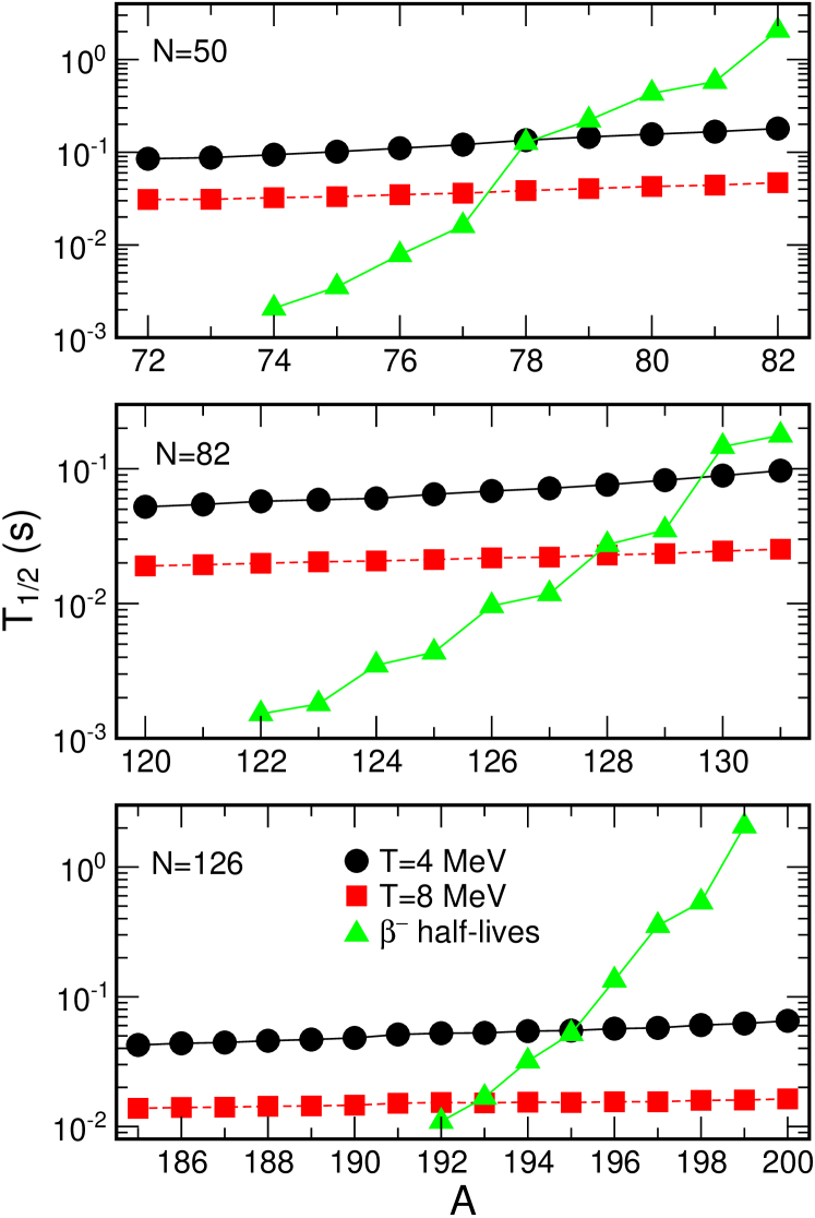
Figure 27: Half-Lives of r-process waiting point nuclei with $N=50$ (top panel), 82 (middle panel) and 126 (bottom panel) against charged-current $(\nu_{e},e^{-})$ reactions. For the neutrinos a Fermi-Dirac distribution with $T=4$ MeV and zero chemical potential (circles) and a luminosity of ($L_{\nu}\sim 10^{52}$ erg s^-1) has been adopted. It is assumed that the reactions occur at a radius of 100 km, measured from the center of the neutron star. The half-lives can be significantly shorter if $\nu_{e}\rightleftarrows\nu_{\mu,\tau}$ oscillations occur. The squares show the half-lives for neutrinos with a Fermi-Dirac distribution with $T=8$ MeV and zero chemical potential, which corresponds to complete $\nu_{e}\rightleftarrows\nu_{\mu,\tau}$ oscillations.

In an environment with large neutrino fluxes the matter-flow to heavier nuclei can also be sped up by charged-current $(\nu_{e},e^{-})$ reactions Nadyozhin and Panov (1993); Qian et al. (1997) which can compete with $\beta$-decays. This is particularly important at the waiting point nuclei associated with $N=50,82$, and 126. Figure 27 shows the $(\nu_{e},e^{-})$ half-lives Hektor et al. (2000); Langanke and Kolbe (2001) for these waiting point nuclei, considering reasonable supernova neutrino parametrizations and assuming that the ejected matter has reached a radius of 100 km. Due to the dependence on $L_{\nu}$ the $(\nu_{e},e^{-})$ half-lives scale with $r^{2}$. Indeed, a comparison with the $\beta$ half-lives (figure 27) shows that $(\nu_{e},e^{-})$ reactions can be faster than the longest $\beta$-decays of the $N=50,82$, and 126 waiting point nuclei, thus speeding up the breakthrough of the matter at the waiting points, if the r-process occurs rather close to the surface of the neutron star. This is even further enforced if $\nu_{e}\rightleftarrows\nu_{\mu,\tau}$ oscillations occur due to the higher energy spectrum of the supernova $\nu_{\mu,\tau}$ neutrinos. However, the presence of charged-current reactions on nuclei in the neutrino-driven wind model implies also neutrino reactions on nucleons strengthening the $\alpha$ effect Meyer et al. (1998).

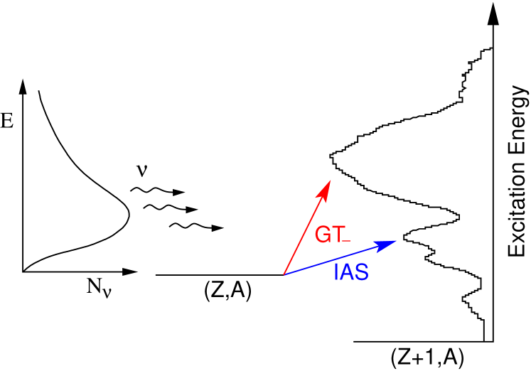
Figure 28: Schematic view of the $(\nu_{e},e^{-})$ reaction on r-process nuclei. Due to the high neutrino energies the cross sections are dominated by transitions to the Fermi (IAS) and Gamow-Teller resonances.

Under a strong neutrino flux the weak flow is determined by an effective weak rate given by the addition of the charged-current $(\nu_{e},e^{-})$ and the nuclear beta-decay rates McLaughlin and Fuller (1997). It has been argued that the solar system r-process abundances provide evidence for the weak steady-flow approximation, which implies that the observed abundances should be proportional to the half-lives of their progenitor nuclei on the r-process path Kratz et al. (1988, 1993). If this is so, the r-process freeze-out must occur at conditions (i.e. radii) at which $\beta$-decay dominates over $(\nu_{e},e^{-})$ reactions, at least for late times. The reason is that neutrino capture on magic nuclei with $N=50,82,126$ is not reduced if compared to the neighboring nuclides, as the capture occurs from a reservoir of neutrinos with sufficiently high energies to allow for transitions to the IAS and GT resonant states (see figure 28). Consequently $(\nu_{e},e^{-})$ cross sections scale approximately like the neutron excess $(N-Z)$, reflecting the Fermi and Ikeda sumrules (see figure 27). However, the observed solar abundances around the $A=130$ ($N=82$) and 195 ($N=126$) peaks do not show such a smooth dependence with $A$ as will be the case if the effective weak rate is dominated by neutrino reactions. If we require that the $\beta$ decay half-lives dominate over the $(\nu_{e},e^{-})$ reactions we can put constraints on the neutrino fluence in the neutrino-driven wind scenario, which is particularly strict if neutrino oscillations occur. If, as an illustrative example, we apply the constraint to the heavy waiting point nuclei with $N=126$ (e.g. the nuclei with $A\sim 199$) and adopt the neutrino and beta half-lives from figure 27, $\beta$-decay is only faster if the neutrino-nucleus reactions occur at distances larger than $\sim 500$ km.

Figure 29: Effect of post-processing by neutrino-induced reactions on the r-process abundance. The unprocessed distribution (solid line) is compared with the distribution after post-processing (dashed line). A constant fluence of ${\cal F}=0.015$ has been assumed, which provides a best fit to the observed abundances for $A=183-87$ (see inset). The observed abundances are plotted as filled circles with error bars (from Qian et al., 1997)).

As the $Q_{\beta}$ values in the very neutron-rich r-process nuclei are large, the IAS and GT resonant states reside at rather high excitation energies ($\sim 20$–30 MeV), in the daughter nuclei for $(\nu_{e},e^{-})$ reactions. This fact, combined with the small neutron separation energies in these nuclei, ensures that $(\nu_{e},e^{-}$) reactions, and also neutral-current $(\nu,\nu^{\prime}$) reactions, spall neutrons out of the target nuclei Haxton et al. (1997); Qian et al. (1997) ($\sim 5$–7 neutrons for nuclei in the $A=195$ mass region Haxton et al. (1997); Hektor et al. (2000)). During the r-process, i.e. as long as the neutron source is strong enough to establish $(n,\gamma)\rightleftarrows(\gamma,n)$ equilibrium, the neutrons will immediately be recaptured leading to no effect on the abundance distribution. However, once the neutron source has ceased, e.g. after freeze-out, and if the r-process matter in the neutrino-driven wind model is still subject to strong neutrino fluxes, neutrons liberated during this phase by neutrino-induced reactions, will not be recaptured and this post-processing Qian et al. (1997); Haxton et al. (1997) leads to changes in the r-process abundance distribution. It is argued Haxton et al. (1997) that due to the smooth dependence of the neutrino cross sections on the mass number, the post-processing, in general, shifts abundances from the peaks to the wings at lower $A$-values (figure 29). This shift depends on the neutrino exposures and allows constraints to be put on the total neutrino fluence in the neutrino-driven wind model Qian et al. (1997); Haxton et al. (1997). The limits obtained this way are compatible with the values predicted by supernova models. Whether $\beta$-delayed neutron emission, which has been neglected in Haxton et al. (1997) might affect the post-processing is an open question Kratz (2001, 2002).

Attempts to include neutrino-induced reactions in the r-process network within the neutrino-driven wind model have been reported in Fuller and Meyer (1995); McLaughlin and Fuller (1995); Terasawa et al. (2001b, a). In particular Meyer et al. (1998) studied the competition of the $\alpha$-effect with the possible speed-up of the matter-flow by charged-current reactions on nuclei. These authors estimated the respective charged-current cross sections for allowed transitions on the basis of the independent particle model. Improving on this treatment, Borzov and Goriely calculated $(\nu_{e},e^{-})$ cross sections for supernova neutrinos (Fermi-Dirac distribution with $T=4$ MeV) within the ETFSI method, consistently with their most recent estimates for the $\beta$ half-lives Borzov and Goriely (2000). RPA-based neutrino-nucleus cross sections for selected nuclei have been reported in Surman and Engel (1998); Hektor et al. (2000). Very recently a tabulation with charged- and neutral-current total and partial neutron spallation cross sections have become available for the neutron-rich r-process nuclei Langanke and Kolbe (2001, 2002). This tabulation is based on the RPA and considers allowed and forbidden transitions. Furthermore, the cross sections are tabulated for various supernova neutrino distributions, thus also allowing study of the influence of complete neutrino oscillations on the r-process.

Figure 30: The lower panel shows the average mass number of heavy seed nuclei $\langle A\rangle$ and the neutron-to-seed ratio (n/Seed) in a neutrino-driven wind simulation with an exponential time dependence of the matter flow, determined by the parameter $\tau_{\text{dyn}}$. The open squares show the results for a simulation including neutrino-nucleus reactions, while the full triangles refer to a study in which the neutrino-reactions on nuclei have been switched off. The upper panel shows the sum of the mass number of the seed nucleus plus the neutron-to-seed ratio. This quantity shows up to which mass number the r-process can produce nuclides. The horizontal lines indicate the second ($A\sim 130$) and third ($A\sim 200$) r-process peaks as well as the position of the smaller r-process peak related to the deformed nuclei in the rare-earth region (REE peak), (courtesy of M. Terasawa).

Terasawa et al. (2001b, a) have performed studies similar to the pioneering work of Meyer et al. (1998), however, using their neutrino-driven wind model and the complete set of RPA neutrino-nucleus reaction rates Langanke and Kolbe (2001, 2002). A typical result is shown in figure 30, where, however, the simplifying, but reasonable assumption of an exponential time-dependence of the matter-flow, governed by the parameter $\tau_{\text{dyn}}$, away from the neutron star has been assumed. The quantity $\langle A\rangle$ defines the average mass of the heavy seed nuclei present at the beginning of the r-process, defined at $T=2.5\times 10^{9}$ K. The neutron-to-seed ratio $n/s$ is very sensitive to the dynamical evolution time. This comes about as the shorter $\tau_{\text{dyn}}$, the less time is available to assemble the seed nuclei from $\alpha$-particles and neutrons. Consequently the abundance of seed nuclei decreases for shorter $\tau_{\text{dyn}}$, increasing the $n/s$ ratio. If the neutrino flux is artificially switched off, matter-flow to the 3rd r-process peak at $A\sim 200$ (2nd r-process peak at $A\sim 130$) is achieved if $\tau_{\text{dyn}}\leq 0.01$ s ($\tau_{\text{dyn}}\leq 1$ s). The consistent inclusion of neutrino reactions is counter-productive to a successful r-process. This effect becomes more dramatic if the matter-flow is slow as then the $\alpha$-effect strongly suppresses the availability of free neutrons at the beginning of the r-process (see also Meyer et al., 1998). No r-process, i.e. no production of nuclides in the second r-process peak at $A\sim 130$, is observed if $\tau_{\text{dyn}}\gtrsim 0.05$ s.

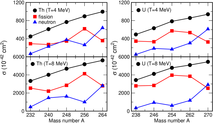
Figure 31: Total $(\nu_{e},e^{-})$ (circles) and partial $(\nu_{e},e^{-}n)$ (triangles) and neutrino-induced fission cross sections (squares) for selected thorium and uranium isotopes. The calculations have been performed for Fermi-Dirac $\nu_{e}$ distributions with temperature $T=4$ MeV and 8 MeV. The first reflects a typical supernova $\nu_{e}$ spectrum, while the latter assumes complete $\nu_{\mu,\tau}\rightarrow\nu_{e}$ neutrino oscillations.

Recently Qian (2002) has suggested that, within the neutrino-driven wind r-process scenario, charged-current neutrino reactions can induce fission reactions on r-process progenitor nuclei heavier than lead and that the fission products account for the observed r-process abundance in metal-poor stars Sneden et al. (2000). These observed abundances show a peak around mass number $A\sim 195$, which follows the solar r-process distribution, and enhanced structures at around $A\sim 90$ and $\sim 132$ which, due to the suggestion of Qian (2002), are fission products, which do not follow a solar r-process pattern. First calculations of neutrino-induced fission cross sections have been performed by Kolbe et al. (2002) using a combination of RPA model, to calculate the $(\nu_{e},e^{-})$ excitation function, and statistical model to determine the final branching probabilities. The neutrino-induced fission cross sections (see figure 31) are quite large as the progenitor nuclei are neutronrich, which increases the Fermi and Gamow-Teller contributions to the total cross sections and places their strengths at energies above the fission barrier in the daughter nucleus. The calculations shown in figure 31 use the fission barriers derived by Howard and Möller (1980). Modern evaluations predict larger fission barriers (e.g. Mamdouh et al., 2001) which would reduce the fission cross section. The cross sections can be significantly enlarged if $\nu_{\mu,\tau}\rightarrow\nu_{e}$ neutrino oscillations occur during the neutrino-driven wind r-process scenario.

VII The Neutrino Process

When the flux of neutrinos generated by the cooling of the neutron star passes through the overlying shells of heavy elements interesting nuclear transmutations are induced, despite the small neutrino-nucleus cross sections. Of particular interest here are neutral-current reactions as they can be induced by $\nu_{\mu},\nu_{\tau}$ neutrinos and their antiparticles with the higher energy spectra ($\langle E_{\nu}\rangle\sim 25$ MeV). These neutrinos are energetic enough to excite the GT resonant state, and more importantly, also the giant dipole resonant states. These states usually reside above particle thresholds and hence decay mainly by proton or neutron emission, generating new nuclides. The neutrino reaction rates are too small to affect the abundances of the parent nuclei, but they can noticeably contribute to the production of the (sometimes much less abundant) daughter nuclei. As a rule-of-thumb, the neutrino process, i.e. the synthesis of nuclides by neutrino-induced spallation in a supernova, can become a significant production process for the daughter nuclide if one wants to explain abundance ratios of parent-to-daughter which exceed about $10^{3}$ Woosley (2001).

The most interesting neutrino nucleosynthesis occurs in the outer burning shells of the massive star which have not been affected by the fatal core collapse in the center when the neutrinos pass through. However, a little later the shock reaches these shells and the matter will be subjected to rather high temperatures initiating fast nuclear reactions involving also the nuclides just produced by the neutrino-induced reactions. Hence studies of the neutrino process depend on various neutrino-nucleus reaction rates and on the neutrino spectra and fluxes, especially of the $\nu_{\mu},\nu_{\tau}$ neutrinos, and they require a rather moderate nuclear network to simulate the effects of the re-processing by the shock. The first investigation of the neutrino process has been reported in Woosley et al. (1990). A more recent study Woosley and Weaver (1995) confirmed the main result that a few specific nuclei (⁷Li, ¹¹B, ¹⁹F) are being made by the neutrino process in significant fractions. For example, ¹¹B and ¹⁹F are being made by $(\nu,\nu^{\prime}p)$ and $(\nu,\nu^{\prime}n)$ (followed by a $\beta$-decay) reactions on the abundant ¹²C and ²⁰Ne, respectively. As noted by Woosley et al. (1990) neutrino nucleosynthesis can also contribute to the production of ¹⁸⁰Ta (see above) and ¹³⁸La. First calculations of the relevant total and partial neutrino-induced cross sections have been reported in Heger et al. (2002), (see also Belic et al., 2002). The nucleus ¹³⁸La is special as it is mainly made by the charged-current reaction ¹³⁸Ba$(\nu_{e},e^{-}){}^{138}$La, while the lighter nuclei (⁷Li, ¹¹B, ¹⁹F) and dominantly also ¹⁸⁰Ta, are being produced by neutral-current reactions induced by $\nu_{\mu},\nu_{\tau}$ neutrinos. The neutrino process is therefore sensitive to $\nu_{e}$ and ($\nu_{\mu},\nu_{\tau}$) neutrinos, which are expected to have different spectra in Type II supernovae (see section V.C), and hence it can test this prediction. Moreover, the ¹³⁸La nucleosynthesis is sensitive to neutrino oscillations, as this nuclide would be significantly overproduced if supernova $\nu_{\mu},\nu_{\tau}$ neutrinos have a noticeably larger average energy and if they oscillate into $\nu_{e}$ neutrinos before reaching the ¹³⁸La production site (helium shell) in massive stars.

Neutrino-induced nucleon spallation on ¹²C can also knock-out a deuteron or a proton-neutron pair, in this way producing ¹⁰B. The expected ¹⁰B/¹¹B abundance ratio in neutrino-nucleosynthesis is $\sim 0.05$, which is significantly smaller than the observed abundance ratio, 0.25 Haxton (2000). Thus there must be a second process which contributes to the production of ^10,11B. These are reactions of energetic protons on ¹²C in cosmic rays, which yield a ratio of ¹⁰B/¹¹B of about 0.5, larger than the observed value. A solution might be that the two nuclides are being produced by both mechanisms, neutrino-nucleosynthesis and cosmic ray spallation. It is interesting to note that the first process, being associated with supernovae, is a primary process, while the latter is a secondary process, as it requires the existence of protons and ¹²C in the interstellar medium. As a consequence the ¹⁰B/¹¹B abundance ratio should have changed during the history of the galaxy. This can be tested once observers are able to distinguish between the abundances of the two different boron nuclides in stellar spectra Haxton (2000).

VIII Binary Systems

Weak processes can also play interesting roles in the evolution and nucleosynthesis processes in close binary systems where one component is a compact object (white dwarf or neutron star) and the other a massive star. If the latter expands during helium core burning, mass flow from the hydrogen envelopment of the star onto the surface of the compact object sets in. If the respective mass accretion rate is rather low ($10^{-8}$–$10^{-10}$ $M_{\odot}$ y^-1), the hydrogen, accreted on the surface of the compact object, burns explosively under degenerate conditions leading to a nova (if the compact object is a white dwarf) or an x-ray burst (neutron star). This means that the energy released by the nuclear reactions is used to heat the matter rather than for expansion. The rise in temperature increases the nuclear reaction rates, triggering a thermonuclear runaway until the degeneracy is finally lifted and an outer layer of matter is ejected. In a type Ia supernova the faster mass accretion rate on to the surface of a white dwarf (likely a carbon-oxygen white dwarf with sub-Chandrasekhar mass $\sim 0.7\ M_{\odot}$) leads to steady hydrogen and subsequently helium burning. If the growing mass of the white dwarf exceeds the Chandrasekhar mass, contraction sets in and the carbon in the center ignites by fusion reactions with screening enhancement. As the environment is highly degenerate, a thermonuclear runaway is triggered which eventually will explode the entire star.

VIII.1 Novae

The main energy source of a nova is the CNO cycle, with additional burning from proton reactions on nuclei between neon and sulfur, if the white dwarf also contained some ²⁰Ne Truran (1982). A nova expels matter which is enriched in $\beta$-unstable ^14,15O for carbon-oxygen white dwarfs (leading to the production of stable ^14,15N nuclides) or can contain nuclides up to the sulfur mass region for neon-oxygen novae Starrfield et al. (1998, 2000); José and Hernanz (1998). The most important role of weak-interaction processes in novae is their limitation of the energy generation during the thermonuclear runaway. An interesting branching occurs at $T\sim 8\times 10^{7}$ K. For lower temperatures the $\beta$-decay of ¹³N with a half-life of $\sim 10$ m dominates over the ¹³N$(p,\gamma)$ reaction and sets the timescale for the nuclear burning. As charged-particle fusion reactions are sensitively dependent on temperature, their reaction rates strongly increase with rising temperature and for $T\geq 8\times 10^{7}$ K and densities of order $10^{4}$ g cm^-3 the proton capture on ¹³N is faster than the $\beta$-decay. The CNO cycle turns into the hot CNO cycle and now the positron decay of ¹⁵O with a half-life of 122 s is the slowest reaction occuring in the CNO nova network. It turns out that, once the degeneracy is lifted, the dynamical expansion timescale is faster than the one for nuclear energy generation, set by the ¹⁵O half-life. As a consequence the runaway is quenched Truran (1982). We mention that the determination of the dominant resonant contribution to the ¹³N$(p,\gamma){}^{14}$O rate has been the first successful application of the Coulomb dissociation technique in nuclear astrophysics Motobayashi et al. (1991).

Weak-interaction rates relevant for nova studies can be derived from either experimental data or shell-model calculations.

VIII.2 X-ray Bursts

An x-ray burst is explained as a thermonuclear runaway in the hydrogen-rich envelope of an accreting neutron star Lewin et al. (1993); Taam et al. (1993). Due to the higher gravitational potential of a neutron star, the accreted matter on the surface reaches larger densities than in a nova (up to a few $10^{6}$ g cm^-3) and the temperature during the runaway can rise up to $2\times 10^{9}$ K Schatz et al. (1998). Under these conditions hydrogen burning is explosively fast. The trigger reactions of the runaway are the triple-alpha reactions and the break-out from the hot CNO cycle, mainly by $\alpha$-capture on ¹⁵O and ¹⁸Ne. We note that these two reaction rates are yet insufficiently known due to uncertain resonant contribution at low energies Mao et al. (1996); Görres et al. (1995). The thermonuclear runaway is driven first by the $\alpha p$ process, a sequence of $(\alpha,p)$ and $(p,\gamma)$ reactions which shifts the ashes of the hot CNO cycle to the Ar and Ca mass region, and then by the rp-process (short for rapid proton capture process). The rp-process represents proton-capture reactions along the proton dripline and subsequent $\beta$-decays of dripline nuclei processing the material from the Ar-Ca region up to ⁵⁶Ni Schatz et al. (1998). The $\beta$ half-lives on the rp-process path up to ⁵⁶Ni are known sufficiently well.

The runaway freezes out in thermal equilibrium at peak temperatures of $(2\text{--}3)\times 10^{9}$ K with an abundance distribution rich in ⁵⁶Ni, forming Ni oceans on the surface of the neutron star. Further matter flow at these temperatures is suppressed due to the low proton separation energy of ⁵⁷Cu and the long half-life of ⁵⁶Ni. Re-ignition of the rp-process then takes place during the cooling phase, starting with proton capture on ⁵⁶Ni and potentially shifting matter up to the ¹⁰⁰Sn region where the rp-process ends in a cycle in the Sn-Te-I range Schatz et al. (2001). A matter flow to even heavier nuclei is possible, if the rp-process operates in a repetitive mannor; i.e. a new rp-process is ignited after the ashes of the previous process have decayed to stability and before these nuclei have sunk too deep into the crust of the neutron star (see below). Such repetitive rp-process models, shortly called $(\rm rp)^{2}$-process, have been studied by Boyd et al. (2002).

The reaction path beyond ⁵⁶Ni runs through the even-even $N=Z$ nuclei which due to their known long half-lives (⁶⁴Ge has a half-life of 63.7(25) s) represent a strong impedance to the matter-flow. This can also not be overcome always by proton captures as for some of the $\alpha$-like nuclei the resulting odd-$A$ nucleus is proton-unbound and exists only as a resonance. Such situations occur, for example, for the ⁶⁸Se$(p,\gamma){}^{69}$Br and ⁷²Kr$(p,\gamma){}^{73}$Rb reactions. It has been suggested Görres et al. (1995) that the gap in the reaction path can be bridged by two-proton captures, with the resonance serving as intermediate state (like in the triple-$\alpha$ reaction). The reaction rate for such a two-step process depends crucially on the resonance energy, with some appropriate screening corrections.

Most half-lives along the rp-process path up to the ⁸⁰Zr region are known experimentally. This region of the nuclear mass chart is known for strong ground state deformations, caused by coupling of the $pf$-shell orbitals to the $g_{9/2}$ and $d_{5/2}$ levels. The strong deformation makes theoretical half-life predictions quite inaccurate, mainly due to uncertainties in the $Q$-values stemming from insufficiently wellknown mass differences. We note that the effective half-life of a nucleus along the rp-process path could be affected by the feeding of isomeric states in the proton captures or by thermal population of excited states in general. Again, deformation plays a major role as then even in $\alpha$-like nuclei excited states are at rather low energies (e.g. the first $2^{+}$ state in ⁸⁰Zr is at 290 keV). Apparently a measurement of the half-lives is indispensable for rp-process studies beyond $A=80$. An important step has recently been taken by measuring the half-life of ⁸⁰Zr at the Holifield Facility in Oak Ridge Ressler et al. (2000). The experimental value of $4.1^{+0.8}_{-0.6}$ s reduces the previous (theoretical) uncertainty considerably and, in fact, it is shorter than the value adopted previously in x-ray bursts simulations. Fast proton captures on the daughter products ⁸⁰Y and ⁸⁰Sr allow matter-flow to heavier nuclei, with the $\alpha$-nucleus ⁸⁴Mo ($N=Z=42$) being the next bottleneck. Experiments to measure this important half-life are in progress.

The nucleosynthesis during the cooling phase in an x-ray burst alters considerably the abundance distribution in the atmosphere, ocean and crust of the neutron star. For example, the rp-process may be a possible contributor to the presently unexplained relatively high observed abundance of light p-nuclei like ⁹²Mo and ⁹⁶Ru Schatz et al. (1998). This assumes that the matter produced in the x-ray burst gets expelled out of the large gravitational potential of the neutron star, which is still questionable. Due to continuing accretion the rp-process ashes are pressed into the ocean and crust of the neutron star, replacing there the neutron star’s original material. When the ashes sink into the crust, they reach regions of higher densities, and relatedly, larger electron chemical potentials. Thus, consecutive electron captures will become energetically favorable and make the ashes more neutron-rich. At densities beyond neutron drip ($\rho\sim(4\text{--}6)\times 10^{11}$ g cm^-3) neutron emissions become possible and at even higher densities pycnonuclear reactions can set in Bisnovatyi-Kogan and Chechetkin (1979); Sato (1979); Haensel and Zdunik (1990). Importantly, these processes (electron capture, pycnonuclear reactions) generate energies which can be locally stored in the neutron star’s ocean and crust and will affect their thermal properties Brown and Bildsten (1998). Previous studies of these processes in accreting neutron stars have assumed that iron is the endproduct of nuclear burning and the sole nucleus reaching the crust of the neutron star (e.g. Haensel and Zdunik, 1990). But clearly the rp-process produces a wide mixture of heavy elements Schatz et al. (1999), where the abundance distribution depends on the accretion rate.

The ashes consist mainly of even-even $N=Z$ nuclei, for which electron capture at neutron star conditions occur always in steps of two. At first, the capture on the even-even nucleus sets in once sufficiently high-energy electrons are available to effectively overcome the $Q_{\text{EC}}$-value to the odd-odd daughter nucleus. Due to nuclear pairing, which favors even-even nuclei, the $Q_{\text{EC}}$-value for the produced daughter nucleus is noticeably lower so that electron capture on the daughter readily follows at the same conditions. The energy gain of the double-electron capture is of order the difference of the two $Q_{\text{EC}}$-values; this gain is split between the emitted neutrino and a local heating. Considering a blob of accreted matter initially consisting solely of ⁵⁶Ni and assuming temperature $T=0$, the evolution of this blob was followed on the neutron star surface until neutron-drip densities and beyond Haensel and Zdunik (1990). The $rp$-process simulations, however, indicate a finite temperature of the ashes of a few $10^{8}$ K, allowing electron capture already from the high-energy tail of the electron distribution and significantly reducing the required densities.

VIII.3 Type Ia Supernovae

Type Ia supernovae at high redshifts serve currently as the standard candles for the largest distances in the universe. Importantly recent surveys of such distant supernovae provide evidence for an accelerating expansion of the universe over the last several $10^{9}$ years Riess et al. (1998); Perlmutter et al. (1999).

Type Ia supernovae have been identified as thermonuclear explosions of accreting white dwarfs with high accretion rates in a close binary system. While the general explosion mechanism is probably understood, several issues are still open like the masses of the stars in the binary or the carbon/oxygen ratio and distribution in the white dwarf. The probably most important problem yet is the modelling of the matter transport during the explosion and the velocity of the burning front, both requiring multidimensional simulations (e.g. Woosley, 2001; Reinecke et al., 1999; Hillebrandt and Niemeyer, 2000).

Figure 32: $Y_{e}$ profile as a function of radial mass for the standard type Ia supernova model WS15 Nomoto et al. (1984) using the FFN and the shell-model weak-interaction rates (LMP), (courtesy of F. Brachwitz).

Figure 33: Ratio of calculated to solar abundances predicted by the WS15 model Nomoto et al. (1984) using the FFN and the shell-model rates (LMP). The ordinate is normalized to ⁵⁶Fe. Intermediate-mass elements exist but are underproduced by a factor of 2–3 for SNe Ia models in comparison to Fe group elements. Using the FFN rates the Fe group does not show a composition close to solar. Especially ⁵⁰Ti and ⁵⁴Cr are strongly overproduced by more than a factor of 3. The change from FFN rates (left) to LMP (right) reduces the overproduction over solar close to the acceptable limit of a factor 2 (courtesy of F. Brachwitz).

Type Ia supernovae contribute about half to the abundance of Fe-group nuclides in galactic evolution. Thus one can expect that type Ia supernovae should not overproduce abundances of nuclides in the iron group, such as ⁵⁴Cr or ⁵⁰Ti, relative to ⁵⁶Fe by more than a factor of two compared with the relative solar abundances. This requirement puts stringent constraints on models, in particular on the central density of the progenitor white dwarf and the flame speed Iwamoto et al. (1999). When the flame travels outwards, it heats the matter to temperatures of a few $10^{9}$ K and brings its composition close to nuclear statistical equilibrium (NSE). As the original matter (¹⁶O, ¹²C) had an electron-to-baryon ratio of $Y_{e}=0.5$, the NSE composition is dominated by ⁵⁶Ni, which after being expelled decays to ⁵⁶Fe. However, behind the flame front, which travels with a few percent of the local sound speed Niemeyer and Hillebrandt (1995), electron captures occur, which lower $Y_{e}$ and drive the matter composition more neutron-rich. This effect is larger the greater the central density of the white dwarf (which increases the electron capture rates) and the slower the flame speed (which allows more time for electron captures). Figure 32 shows the $Y_{e}$ profile obtained in a standard type Ia model WS15 Nomoto et al. (1984), with slow deflagration flame speed (1.5% of sound velocity), central ignition density $\rho=2.1\times 10^{9}$ g cm^-3 and a transition from deflagration to detonation at density $\rho=2.1\times 10^{7}$ g cm^-3. The calculations have been performed by Brachwitz (2001) with the FFN Fuller et al. (1982b) and shell model Langanke and Martínez-Pinedo (2001) weak interaction rate sets. The differences are quite significant, even if one considers that about $60\%$ of the captures occur on free protons, which are unaffected by the differences in these rate sets. Under otherwise identical conditions the slower shell model rates yield a central $Y_{e}$ value of 0.45, which is about 0.01 larger than for the FFN rates. Consequently very neutron-rich nuclei with $Y_{e}\leq 0.45$ are significantly suppressed (see figure 33). In fact, no nuclide is significantly overproduced in this model compared to the solar abundance. The net effect of the new rates is that, for an otherwise unchanged model, it increases the central density by about a factor of 1.3 Brachwitz et al. (2000); Woosley (2001). This can have quite interesting consequences if one wants to use the nucleosynthesis constraint to distinguish between two quite distinct type Ia models. On the basis of recent models it has been concluded that the majority of type Ia progenitors grow towards the Chandrasekhar mass through steady hydrogen and helium burning Hachisu et al. (1999). Such systems would lead to rather low central densities $\rho\leq 2\times 10^{9}$ g cm^-3. In these models, only a small fraction of progenitors would deviate from steady hydrogen burning at the end of the accretion history experiencing weak hydrogen flashes; such cases correspond to the W-model discussed above yielding higher central densities. We stress, however, that changes in the nucleosynthesis caused by differences in the central densities in the models can be counterbalanced by changes of the flame speed.

IX Conclusions and future perspectives

It has long been recognized that nuclear weak-interaction processes play essential roles in many astrophysical scenarios. In a few cases these are specific reactions, which are particularly important, and these reactions have then been studied with increasingly refined models. Examples are the various weak-interaction processes in the solar hydrogen burning chains including the initial $p+p$ fusion reaction Kamionkowski and Bahcall (1994); Park et al. (1998); Park et al. (2001a); Kong and Ravndal (2001) or the very challenging ${}^{3}\text{He}+p$ reaction Marcucci et al. (2001); Park et al. (2001b); Marcucci et al. (2000), which generates the highest-energy neutrinos in the sun. Another typical example is the solar electron capture rate on ⁷Be, where the nuclear matrix element can be determined from the experimental lifetime of atomic ⁷Be, while the proper description of the solar plasma effects on the capture rate with the desired accuracy has been quite demanding.

However, most astrophysical applications require the knowledge of weak-interaction rates for a huge body of nuclei. If, like for s-process nucleosynthesis, the nuclei involved are close to the valley of stability and hence quite long-lived, the needed rates (usually half-lives) have been determined experimentally in decade-long efforts. For the s-process the challenge now focuses on the branching point nuclei where the reaction flow branches into two (or more) paths and where, in some cases, the observed relative abundances of nuclides along the different paths depend on the stellar conditions (temperature, neutron density) and hence allow determination of these quantities inside the star. Again, the approach is to measure the necessary data, e.g. half-lives of excited nuclear states.

Other astrophysical scenarios involve nuclei far-off stability, often under extreme conditions (high density, neutron flux, temperature). These astrophysical sites include core-collapse (type II) and thermonuclear (type Ia) supernovae, r-process nucleosynthesis and explosive hydrogen burning; and the interest in all of these has been boosted recently by novel observations and data (supernova 1987A, high-redshift supernova survey, Hubble Space Telescope, …). A direct experimental determination of the respective stellar weak-interaction rates has been possible in a few cases, like the half-lives of r-process and rp-process waiting point nuclei. However, in nearly all cases the weak-interaction processes had to be theoretically modeled so far – a very demanding job if one considers that often results for many hundreds of nuclei for a large range of stellar conditions are needed. These data were then derived globally based on parametrized nuclear structure arguments, as an appropriate treatment of the involved nuclear structure problem was prohibited by both the available computational capabilities and the lack of experimental guidance. Although evaluation of rate sets for astrophysical purposes often appears to be a theoretical problem, the second point – experimental guidance – is crucial and often overlooked. It is Willy Fowler’s strategy and legacy that nuclear models used to derive nuclear ingredients in astrophysical applications, should be consistent, but more importantly they should be accurate and, as a consequence, experimental data are to be used whenever available. Therefore the role of experimental data in nuclear astrophysics is twofold: If possible, they supply the needed information directly, or equally important, they constitute constraints and guidance for the nuclear models from which the needed information is obtained. Thus, the renaissance of nuclear structure, which we have witnessed in recent years, has two consequences in nuclear astrophysics. The recent development of new facilities, techniques and devices brought a large flood of new experimental information, in particular for the proton- and neutron-rich nuclei away from stability. These data indicate that the nuclear structure models adopted to derive the global data and rate sets were usually too simple and improvements were warranted. The experimental renaissance went hand-in-hand with decisive progress in nuclear structure theory, made possible by the development of new models and better computer hardware and software. Due to both experimental and theoretical advances, it becomes now possible to calculate nuclear data sets for astrophysical applications on the basis of realistic models rather than on crude and often oversimplified parametrizations. This review presents a summary of recent theoretical calculations.

The advances in nuclear structure modelling have also lead to progress in astrophysically important nuclear input other than weak-interaction processes. Typical examples are the equation of state, derived on the basis of the relativistic mean-field model guided by the relativistic Brückner-Hartree-Fock theory Shen et al. (1998a, b), which serves as an alternative to the standard Lattimer-Swesty EOS Lattimer and Swesty (1991), or the nuclear mass table and level density parametrizations determined within the framework of the Hartree-Fock model with BCS pairing Goriely et al. (2001); Demetriou and Goriely (2001). Such mass tables, or equivalently neutron separation energies, play an essential role in r-process nucleosynthesis and are conventionally derived by parametrizations constrained to known masses.

Other astrophysical areas, loosely or indirectly related to the topic of this review, have also benefitted from the progress in modelling nuclear weak-interaction processes. A field with rapidly growing importance is Gamma-ray Astronomy with beta-unstable nuclei. Due to $\gamma$-ray observatories in space it has been possible in recent years to search the sky for sources of known $\gamma$-rays which can then be associated with recent nucleosynthesis activities. A highlight has been the observation of the 1.157 MeV $\gamma$-line, produced in the $\beta$-decay scheme of ⁴⁴Ti, in the Cassiopeia supernova remnant Iyudin et al. (1994). Knowing the date of the supernova, the ⁴⁴Ti half-life, the distance to the source and the measured intensity of the $\gamma$-line allows determination of how much ⁴⁴Ti has been ejected into the interstellar medium by the supernova event. Furthermore, as $\gamma$-rays can, in contrast to optical wave lengths, escape from the galactic bulk, $\gamma$-ray observation allows to detect historical supernovae which have not been observed optically Iyudin et al. (1998), (also observed in x-rays by Aschenbach, 1998). Such searches for historical supernovae and an improved determination of the supernova frequency in our galaxy will be one of the main missions of future $\gamma$-ray observatories in space, like INTEGRAL. A longer-lived radioactive nuclide produced in supernovae is ⁶⁰Fe. Investigations of rock samples taken from the ocean floor, by precision accelerator mass spectroscopy, found a significant increase of ⁶⁰Fe abundance compared to other iron isotopes pointing to a close-by supernova about 5 million years ago Knie et al. (1999).

Weak-processes on nuclei and electrons are the means to observe solar and supernova neutrinos Balantekin and Haxton (1999). Solar neutrinos have rather low energies ($E_{\nu}\leq 14$ MeV) and hence induce specific low-lying transitions which are theoretically modelled best by shell-model calculations. Applications have been performed, for example, for ³⁷Cl Aufderheide et al. (1994a), ⁴⁰Ar Ormand et al. (1995) and ⁷¹Ga Haxton (1998), the detector material in the Homestake Cleveland et al. (1998), ICARUS, and GALLEX/SAGE/GNO detectors Hampel et al. (1999); Abdurashitov et al. (1999); Altmann et al. (2000), respectively. Supernova neutrinos have higher energies; in particular, the energies of $\mu,\tau$ neutrinos and antineutrinos are expected to be high enough to excite the giant dipole resonances in nuclei. Studies for detector materials like Na, Fe, Pb have been performed in hybrid approaches combining shell model calculations for allowed transitions with the RPA model for forbidden transitions or treating the forbidden transitions on the basis of the Goldhaber-Teller model Fuller et al. (1999); Kolbe and Langanke (2001).

Despite the experimental and theoretical progress, lack of knowledge of relevant or accurate weak-interaction data still constitutes a major obstacle in the simulation of some astrophysical scenarios today. This refers mainly to type II supernovae and r-process nucleosynthesis.

Core-collapse supernovae, as the breeding places of carbon and oxygen, and hence life, in the universe, attract currently significant attention and the quest to definitely identify the explosion mechanism is on the agenda of several international and interdisciplinary collaborations. While most of the efforts concentrate on computational developments towards a multidimensional treatment of the hydrodynamics and the neutrino transport, some relevant and potentially important nuclear problems remain. The improved description of weak-interaction rates in the iron mass range has lead to significant changes in the presupernova models. Evaluation of electron capture rates for heavier nuclei will be available in the near future. First results imply that capture on heavy nuclei, usually ignored in collapse simulations, can compete with the capture on free protons. Whether the inclusion of this process then leads to changes in the collapse trajectory has yet to be seen. Further, finite temperature neutrino-nucleus rates will also soon be available. This will then test whether inelastic neutrino scattering on nuclei, yet not modelled in the simulations, influences the collapse dynamics or supports the revival of the shock wave by preheating of the infalling matter after the bounce. The largest nuclear uncertainty in collapse simulations are likely associated with the description of nuclear matter at high density, extreme isospin and finite temperature. In particular a reliable description of the neutrino opacity in nuclear matter might very well be what is needed for successful explosion simulations. Nucleon-nucleon correlations have been identified to strongly influence the neutrino opacities and nuclear models like the RPA are quite useful to guide the way. Ultimately one would like to see the many-body Monte Carlo techniques, which have been so successfully applied to few-body systems or the nuclear shell model, extended to the nuclear matter problem. First steps along these lines have been reported by Schmidt and Fantoni (1999) and Fantoni et al. (2001), who proposed a novel constrained-path Diffusion Monte Carlo model to study nuclear matter at temperature $T=0$. The Shell Model Monte Carlo model, formulated in momentum space and naturally at finite temperature, constitutes an alternative approach. First attempts in this direction have been taken by the Caltech group Zheng (1996) and by Rombouts (1998). Whether the notorious sign-problem in the SMMC approach can also be circumvented for nuclear matter has still to be demonstrated. Müller et al. (2000) have investigated whether nuclear matter can be formulated on a spatial lattice with nearest neighbor interactions, similar to the Hubbard model for high-$T_{c}$ superconductors. Besides these theoretical efforts it is equally important to improve our understanding of the nuclear interaction in extremely neutron-rich nuclei (matter).

Despite four decades of intense research, the astrophysical site of the r-process nucleosynthesis has yet not been identified. Recent astronomical and meteoric evidence points now to more than one source for the solar r-process nuclides, and it is clearly a major goal in the astrophysics community to solve this cosmic riddle. However, the puzzle will not be definitely solved if the nuclear uncertainties involved are not removed. This is even more necessary as recent research shows that the r-process is a dynamical process under changing astrophysical conditions. This implies dynamically changing r-process paths. To determine the paths one needs to know the masses of nuclei far-off stability accurately, besides the condition of the astrophysical environment. In a dynamical r-process, the astrophysical timescale will compete with the nuclear timescale, i.e. with the time needed for the matter flow from the seed nuclei to the heavier r-process nuclides. This nuclear timescale is set by the half-lives of the nuclei along the paths, in particular by those of the longer-lived waiting point nuclei associated with the magic neutron numbers. The half-lives of waiting point nuclei are a very illustrative example for the need of reliable experimental data: Modern global theoretical models predict half-lives at the waiting points with a spread of nearly one order of magnitude and only data can decide. For the $N=50$ and $N=82$ waiting points such data exist for a few key nuclides (e.g. Pfeiffer et al., 2001), but not for the $N=126$ nuclei.

R-process nucleosynthesis as well as other astrophysical processes will tremendously benefit from future experimental developments in nuclear physics. Worldwide radioactive ion-beam facilities, with important and dedicated programs in nuclear astrophysics, have just started operation or are under construction or in the proposal stage. These new facilities will boost our knowledge about nuclei far-off stability, they will determine astrophysically relevant nuclear input directly (e.g. masses and half-lives for the r-process, half-lives and cross sections for the rp-process, etc). But equally important, the radioactive ion-beam facilities will guide and constrain the nuclear models, in this way indirectly contributing to the reduction of the nuclear inaccuracies in astrophysical models. Ultimatively nuclear physics can and will then become a stringent test and guidance for astrophysical theories and ideas.