Bethe–Salpeter Approach with the Separable Interaction for the Deuteron.

S.G. Bondarenko,1 V.V. Burov,1,3 A.V. Molochkov,1,3 G.I. Smirnov,2 H. Toki 3

1 Bogoliubov Laboratory of Theoretical Physics
Joint Institute for Nuclear Research, Dubna, Russia
2 Laboratory of Particle Physics
Joint Institute for Nuclear Research, Dubna, Russia
3 Research Center for Nuclear Physics
Osaka University, Osaka, 567-0047, Japan
Abstract

Recent developments of the covariant Bethe–Salpeter (BS) approach with the use of the separable interaction for the deuteron are reviewed. It is shown that the BS formalism allows a covariant description of various electromagnetic reactions like the lepton-deuteron scattering, deuteron electro-disintegration, deep inelastic scattering (DIS) of leptons on light nuclei. The procedure of the construction of the separable nucleon-nucleon ($NN$) interaction is discussed. The BS formalism facilitates analysis of the role of the $P$-waves (negative energy components) in the electromagnetic properties of the deuteron and its comparison with the nonrelativistic results. Furthermore the covariant BS approach makes it possible to analyze DIS of leptons from the deuteron in a model independent way and to extend the formalism to DIS reactions on the light nuclei.

1 Introduction

The study of electromagnetic properties of light nuclei, $A\leq 4$, facilitates the construction of the theory of strong interactions and, in particular, the nucleon–nucleon interaction (see, for example, [1]). Theoretical research in this field is of topical interest which is reflected in recent review articles [2]-[7]. A large amount of available experimental data stimulate a further development of theoretical methods which are often restricted to qualitative predictions. The forthcoming experiments are expected to provide high precision data which will allow us to explore the region of large momentum transfer in elastic, inelastic and deep inelastic (DIS) electron-nucleus reactions.

These data will be able to furnish qualitatively new information about the fine nuclear structure at small distance. This is the reason why the role of the non-nucleon degrees of freedom as mesons, $\Delta$-isobars, quarks etc. on intermediate and high energy phenomena is widely discussed (see, for example,  [8]-[21]). Clear understanding and consistent interpretation of the experimental information is not possible without the consideration of the relativistic kinematics of reactions and the dynamics of the interaction. For this reason, the construction of a covariant approach and a detailed analysis of relativistic effects in electromagnetic reactions with light nuclei become the tasks of the highest priority.

One can identify three steps for the construction of a theoretical framework of the lepton–nucleus interaction. The first step is to introduce the dynamical degrees of freedom parameterizing hadronic and nuclear structure. The second one is to construct from these degrees of freedom bound states which are hadrons and nuclei. The third step is to find a formalism of the interaction of these degrees of freedom with incident particles which are photons $\gamma$ and leptons $l$ in the present study.

In some sense this division is artificial, since the three steps are just different parts of the same problem of dynamics of interacting fields to be solved in one consistent approach. The problems are interrelated by the underlying physics in such a way that by fixing one of them one can find solutions for the others. Nevertheless, such a division helps us to separate the task within a consistent set of approximations and to use a phenomenological technique to set constrains on different parts of the approach.

The fact that nuclei consist of bound nucleons introduces a major problem for theoretical description of relativistic $l-A$ interactions. The deuteron is naturally the first object in the row of many other nuclei, and has received a vast number of treatments within many different approaches. One finds also that non-relativistic schemes of calculations are widely employed in the analysis, which can be justified for a few particular cases. On the other hand, the consistent consideration of the relativistic bound states is offered within the Bethe-Salpeter (BS) formalism [22, 23], which makes it most promising for the class of the tasks considered in the present review. What is even more important is that the BS formalism allows qualitatively a new interpretation of the physics of the relativistic bound state and should not be regarded as an alternative scheme only.

The first practical applications of the BS formalism were based on the three dimensional reduction. The first reduction of the BS formalism, the so-called quasi-potential equation, has been made in several works [1],[24]-[37]. The main idea behind these approaches is to fix the relative time of bound constituents to a certain value. Since the relative time (or relative energy in momentum space) is considered as an unphysical feature of the BS formalism, the different ways of fixing the relative time should produce equivalent quasipotential approaches. The comparison of the different quasipotential equations was done in review articles [4, 5]. This line of realization of the BS formalism allows one to take into account some of the relativistic effects, but it looses the general relativistic covariance [38] (see, papers [39, 41] also). Moreover, a number of difficulties arises which does not allow one to establish a direct link to the non-relativistic calculations, for example, the absence of a non-relativistic reduction of arbitrary kernels, the problem of the interpretation of the abnormal parity states. This fact motivates us to use the original BS formalism which offers a consistent covariant description of the interacting particles and their bound states. The qualitative connection with the nonrelativistic results can be made on the level of observables. Such exotic features of the BS formalism as relative time of the bound constituents and abnormal parity states receive their nonrelativistic interpretation through the relation to dynamical degrees of freedom. Analysis of the relative time dependence gives qualitatively a new point of view on relativistic bound states.

This review is devoted to the analysis of the three steps considered above within the Bethe-Salpeter formalism and its application to the study of the electromagnetic properties of light nuclei. We emphasize the covariant description of the BS formalism by taking the separable interaction, which is still a stage of infancy. In particular, the role of the abnormal parity states, in not yet confronted with experimental data, though the necessity is demonstrated in this paper. The review is divided into 6 sections. In section 2, we consider basic properties and definitions of the Bethe-Salpeter formalism. By using an example of the $NN$ system we discuss the basic properties of the four dimensional ($4D$) bound states. In section 3, we investigate the simplest process for such a study — elastic scattering of electrons off the deuteron. In section 4, we discuss the application of the BS formalism to the problem of the deuteron electro-disintegration, which is an inelastic process with finite momentum transfer. The analysis of the deep inelastic scattering of leptons on the lightest nuclei — $A=2\ldots 4$ is presented in section 5. The consideration of the DIS reaction in the infinite momentum frame leads to many simplifications in the analysis and allows us to understand clearly some of the important physical consequences of the $4D$ consideration and to draw model independent conclusions. Section 6 is devoted to the summary of the results of the $4D$ BS formalism.

2 Bethe–Salpeter Approach

2.1 Formalism

In study of processes, involving bound states, in local field theory we have to consider particles which are not asymptotically free. The standard field theory reduction technique gives a way to extract all the information about physical states contained in the matrix elements to a product of field operators (see for example  [42]). However, this technique is based on the assumption that the physical states in the matrix elements can be treated as being asymptotically free, and the interaction is switched on adiabatically. Therefore, bound states are excluded from consideration. In order to include bound states, the reduction formalism must be supplemented by a procedure allowing expectation values in such states to be expressed in terms of vacuum expectation values.

This problem is solved in the nonrelativistic field theory by introducing an external classical field which allows the bound state dynamics to be described as a particle motion in a potential well. As a result, the calculation of the expectation value in a bound state reduces to the calculation of the expectation value in a one-particle state, and binding effects are taken into account by introducing the momentum distribution of this particle. This simple approach can be used to obtain amplitudes of the lepton scattering off bound states in the form of convolution. However, in this case, the role played by relativistic corrections and off-shell effects remains unclear. In quasipotential approaches, the solution of the bound state problem reduces to deriving an analog of the Shrödinger equation with a covariant three-dimensional potential [26]-[31]. The calculation of expectation values in bound states should be essentially the same as in the nonrelativistic case. However, in contrast to nonrelativistic approaches, the quasipotential method allows a qualitative study of the role of the relativistic and the off-shell effects.

A method of calculating the expectation values of $\rm T$-products of local operators in bound states was suggested in [23]. The essence of the method is that the expectation values in bound states are expressed in terms of the vacuum expectation values of a ${\rm T}$-product of local operators and the matrix elements for the transition between the vacuum and the bound state. We shall consider the application of this method to processes involving a bound state of $n$ nucleons.

2.2 The Bethe–Salpeter Amplitude

A consideration of a scattering process is based on the analysis of the matrix element of a ${\rm T}$-product of local operators $\eta_{1}(y_{1})\dots\eta_{k}(y_{k})$ in the initial $A$ and final $A^{\prime}$ bound states. :

$$\langle A^{\prime}(\alpha^{\prime},P^{\prime})|{\rm T}(\eta_{1}(y_{1})\dots\eta_{k}(y_{k}))|A(\alpha,P)\rangle.$$ (1)

$P$ and $P^{\prime}$ are the initial and final momenta of the bound state while the $\alpha$ and $\alpha^{\prime}$ are full sets of their discrete quantum numbers. The local field operators, ${\eta_{i}(y_{i})}$, are current operators determining the nucleon interactions with external fields. To express this matrix element in terms of vacuum expectation values we shall use the fact that in a definite kinematical region the joint propagation of $n$ interacting nucleons occurs via the formation of a bound state. In this case the first term of the series expansion of the $n$-nucleon Green’s function in intermediate state has the form:

$\displaystyle\langle 0|{\rm T}(\Psi(x_{1})\dots\Psi(x_{n})\overline{\Psi}(x^{\prime}_{1}))\dots\overline{\Psi}(x^{\prime}_{n})|0\rangle=$
$\displaystyle=\int\frac{d^{3}P}{(2\pi)^{3}}\sum\limits_{\alpha}\langle 0|{\rm T}(\Psi(x_{1})\dots\Psi(x_{n}))|A(\alpha,P)\rangle\times$
$\displaystyle\times\langle A(\alpha,P)|{\rm T}(\overline{\Psi}(x^{\prime}_{1})\dots\overline{\Psi}(x^{\prime}_{n}))|0\rangle\theta(min\{|{x_{0}}_{i}|\}-max\{|{x^{\prime}_{0}}_{i}|\})+\dots.$ (2)

The functions $\Psi$ and $\overline{\Psi}$ are nucleon field operators in the Heinsenberg representation. The $\theta$ function is arising due to the expansion of the $\rm T$-product in the matrix elements. This function ensures that the causality condition is satisfied:

$$min\{{x_{0}}_{i}\}>max\{{x^{\prime}_{0}}_{i}\}.$$

The extreme values (minimum and maximum) of the nucleon coordinates can be determined by introducing the average coordinate of $n$ fields conjugate to the total momentum $P$, which in the case of $n$ particles of the same mass has the form,

$$X=\frac{\sum\limits_{i}^{n}x_{i}}{n}.$$ (3)

The nucleon coordinates relative to this point are $\tilde{x}_{i}=x_{i}-X$. As a result, the maximum and minimum coordinates can be defined as

$\displaystyle max\{{x_{0}}_{i}\}=X_{0}+max\{|\tilde{x_{0}}_{i}|\},$
$\displaystyle min\{{x_{0}}_{i}\}=X_{0}-max\{|\tilde{x_{0}}_{i}|\}.$ (4)

Using the integral representation of the $\theta$ function

$$\theta(x_{0})=\frac{i}{2\pi}\int\limits_{-\infty}^{+\infty}\frac{e^{-ip_{0}x_{0}}}{p_{0}+i\delta}dp_{0},$$ (5)

we obtain the necessary expression relating the vacuum expectation value of the nucleon operators and the matrix elements for the transition from the vacuum to the bound state:

$\displaystyle\langle 0|{\rm T}(\Psi(x_{1})\dots\Psi(x_{n}))\overline{\Psi}(x^{\prime}_{1})\dots\overline{\Psi}(x^{\prime}_{n})|0\rangle=\sum_{\alpha}\int\frac{d^{3}P}{(2\pi)^{3}}\frac{dP_{0}}{2\pi}e^{-i(P_{0}-E)(X_{0}-X_{0}^{\prime})}\times$ (6)
$\displaystyle\times e^{i(P_{0}-E)(max\{|{\tilde{x}_{0i}}|\}+max\{|{\tilde{x}^{\prime}_{0i}}|\})}\frac{\langle 0|{\rm T}(\Psi(x_{1})\dots\Psi(x_{n}))|A(\alpha,P)\rangle\langle A(\alpha,P)|{\rm T}(\Psi(x^{\prime}_{1})\dots\Psi(x^{\prime}_{n}))|0\rangle}{P_{0}-E+i\delta}.$

This expression is inconvenient because of using two sets of coordinates simultaneously, $\{x_{i}\}$ and $\{X,\tilde{x}_{i}\}$. To avoid this, we shall change over to using the second set of coordinates everywhere in the calculations. Owing to the translational invariance, the following relation holds for the fields $\Psi$:

$\displaystyle\Psi(x+\tilde{x})=e^{i\hat{P}x}\Psi(\tilde{x})e^{-i\hat{P}x}.$ (7)

Replacing $x_{i}$ by $X+\tilde{x}_{i}$ in the operators $\Psi$ and $\overline{\Psi}$ and shifting by $X$, using transformation (7), we obtain the matrix elements for the transition from the vacuum to the bound state in the space of relative nucleon locations:

$\displaystyle\langle 0|{\rm T}(e^{i\hat{P}X}\Psi(x_{1})e^{-i\hat{P}X}\dots e^{i\hat{P}X}\Psi(x_{n})e^{-i\hat{P}X})|A(\alpha,P)\rangle=\Phi^{A(\alpha,P)}(\tilde{x}_{1},\dots\tilde{x}_{n})e^{-i(EX_{0}-{\bf P\cdot X})},$
$\displaystyle\langle A(\alpha,P)|{\rm T}(e^{i\hat{P}X}\overline{\Psi}(x^{\prime}_{1})e^{-i\hat{P}X}\dots e^{i\hat{P}X}\overline{\Psi}(x^{\prime}_{n})e^{-i\hat{P}X})|0\rangle=\overline{\Phi}^{A(\alpha,P)}(\tilde{x}^{\prime}_{1},\dots\tilde{x}^{\prime}_{n})e^{i(EX_{0}-{\bf P\cdot X})}.$ (8)

Although the functions $\Phi^{A(\alpha,P)}$ formally depend on $n$ variables, only $n-1$ of them are independent, owing to the equation $\sum\limits_{i}^{n}\tilde{x}_{i}=0.$ As a result of these transformations, Eq. (6) takes the form:

$\displaystyle\langle 0|{\rm T}(\Psi(x_{1})\dots\Psi(x_{n})\overline{\Psi}(x^{\prime}_{1})\dots\overline{\Psi}(x^{\prime}_{n}))|0\rangle=\sum_{\alpha}\int\frac{d^{4}P}{(2\pi)^{4}}e^{-iP(X-X^{\prime})}\frac{\Phi^{A(\alpha,P)}(\tilde{x}_{1},\dots\tilde{x}_{n})\overline{\Phi}^{A(\alpha,P)}(\tilde{x}^{\prime}_{1},\dots\tilde{x}^{\prime}_{n})}{P_{0}-E+i\delta}.$ (9)

Since the integral with respect to $P_{0}$ is determined by the behavior of the integrand near the pole $P_{0}=E$, we have omitted the exponential factor $exp\{i(P_{0}-E)(max\{|{\tilde{x}_{0i}}|\}+max\{|{\tilde{x}^{\prime}_{0i}}|\})\}$.

The unknown functions $\Phi^{A(\alpha,P)}$ and $\overline{\Phi}^{A(\alpha,P)}$

$\displaystyle\Phi^{A(\alpha,P)}(x_{1},\dots x_{n})=\langle 0|{\rm T}(\Psi(x_{1})\dots\Psi(x_{n}))|A(\alpha,P)\rangle,$
$\displaystyle\overline{\Phi}^{A(\alpha,P)}(x^{\prime}_{1},\dots x^{\prime}_{n})=\langle A(\alpha,P)|{\rm T}(\overline{\Psi}(x^{\prime}_{1})\dots\overline{\Psi}(x^{\prime}_{n}))|0\rangle,$ (10)

introduced above and entering into the matrix elements for the transition from the vacuum to the bound state in Eq. (10) describe the nuclear state in terms of the degrees of freedom of the virtual nucleons. These functions are called the Bethe–Salpeter amplitudes. They give the solution of the fundamental problem — the expression of the expectation values in bound states in terms of the vacuum expectation values.

2.3 Analysis of the Matrix Elements in the BS Formalism

In order to explain how the matrix element (1) is related to the nucleon Green’s functions and the Bethe–Salpeter amplitudes, we consider the matrix element

$$\langle 0|{\rm T}(\Psi(x_{1})\dots\Psi(x_{n})\eta_{1}(y_{1})\dots\eta_{k}(y_{k})\overline{\Psi}(x^{\prime}_{1})\dots\overline{\Psi}(x^{\prime}_{n}))|0\rangle$$ (11)

near the singularity of the $n$-nucleon bound state at $P^{2}=M^{2}$. We expand the time-ordered product in the matrix element (1) in a product of matrix elements of $\Psi$, $\eta$, $\overline{\Psi}$. In order to do this, we choose the maximum and minimum zeroth components from the set $\{x_{i}\}$ in accordance with (4) and keeping only terms which correspond to the first term in (2) we write the $\rm T$-product in the form:

$\displaystyle{\rm T}(\Psi(x_{1})\dots\Psi(x_{n})\eta_{1}(y_{1})\dots\eta_{k}(y_{k})\overline{\Psi}(x^{\prime}_{1})\dots\overline{\Psi}(x^{\prime}_{n}))=$
$\displaystyle={\rm T}(\Psi(x_{1})\dots\Psi(x_{n})){\rm T}(\eta_{1}(y_{1})\dots\eta_{k}(y_{k})){\rm T}(\overline{\Psi}(x^{\prime}_{1})\dots\overline{\Psi}(x^{\prime}_{n}))\times$
$\displaystyle\times\theta(X_{0}-Y_{0}-max\{|{\tilde{x}_{0i}}|\}-max\{|{\tilde{y}_{0i}}|\})\theta(Y_{0}-X^{\prime}_{0}-max\{|{\tilde{x}^{\prime}_{0i}}|\}-max\{|{\tilde{y}_{0i}}|\})+$
$\displaystyle+{\rm T}(\overline{\Psi}(x^{\prime}_{1})\dots\overline{\Psi}(x^{\prime}_{n})){\rm T}(\eta_{1}(y_{1})\dots_{k}\eta(y_{k})){\rm T}(\Psi(x_{1})\dots\Psi(x_{n}))\times$
$\displaystyle\times\theta(X^{\prime}_{0}-Y_{0}-max\{|{\tilde{x}^{\prime}_{0i}}|\}-max\{|{\tilde{y}_{0i}}|\})\theta(Y_{0}-X_{0}-max\{|{\tilde{x}_{0i}}|\}-max\{|{\tilde{y}_{0i}}|\}).$

Inserting a complete set between $\rm T$-products, we rewrite Eq. (1) as a sum over states from the complete set:

$\displaystyle\langle 0|{\rm T}(\Psi(x_{1})\dots\Psi(x_{n})\eta_{1}(y_{1})\dots\eta_{k}(y_{k})\overline{\Psi}(x^{\prime}_{1})\dots\overline{\Psi}(x^{\prime}_{n}))|0\rangle=$
$\displaystyle=\sum_{R,R^{\prime}}\langle 0|{\rm T}(\Psi(x_{1})\dots\Psi(x_{n}))|R\rangle\langle R|{\rm T}(\eta_{1}(y_{1})\dots\eta_{k}(y_{k}))|R^{\prime}\rangle\times$
$\displaystyle\times\langle R^{\prime}|{\rm T}(\overline{\Psi}(x^{\prime}_{1})\dots\overline{\Psi}(x^{\prime}_{n}))|0\rangle\theta(X_{0}-Y_{0}-max\{{|\tilde{x}_{0i}}|\}-max\{|{\tilde{y}_{0i}}|\})\times$
$\displaystyle\times\theta(Y_{0}-X^{\prime}_{0}-max\{|{\tilde{x}^{\prime}_{0i}}|\}-max\{|{\tilde{y}_{0i}}|\})+$
$\displaystyle+\sum_{R,R^{\prime}}\langle 0|{\rm T}(\overline{\Psi}(x^{\prime}_{1})\dots\overline{\Psi}(x^{\prime}_{n}))|R\rangle\langle R|{\rm T}(\eta_{1}(y_{1})\dots\eta_{k}(y_{k}))|R^{\prime}\rangle\times$
$\displaystyle\times\langle R^{\prime}|{\rm T}(\Psi(x_{1})\dots\Psi(x_{n}))|0\rangle\theta(X^{\prime}_{0}-Y_{0}-max\{|{\tilde{x}^{\prime}_{0i}}|\}-max\{|{\tilde{y}_{0i}}|\})\times$
$\displaystyle\times\theta(Y_{0}-X_{0}-max\{|{\tilde{x}_{0i}}|\}-max\{|{\tilde{y}_{0i}}|\})~{},$ (12)

where $\sum\limits_{R,R^{\prime}}$ denotes a summation over discrete quantum numbers and an integration over continuous variables.

Since we are interested in the behavior of Eq. (1) near the pole at $P^{2}=M^{2}$, it is sufficient to study the contribution to Eq. (12) from the lowest bound state corresponding to this pole. The bound state corresponds to the first term of the series (12) with $R=A(\alpha,P)$ and $R^{\prime}=A^{\prime}(\alpha^{\prime},P^{\prime})$. Using the integral representation (5) for the $\theta$ function, we obtain the following expression for the matrix element (11):

$\displaystyle\langle 0|{\rm T}(\Psi(x_{1})\dots\Psi(x_{n})\eta_{1}(y_{1})\dots\eta_{k}(y_{k})\overline{\Psi}(x^{\prime}_{1})\dots\overline{\Psi}(x^{\prime}_{n}))|0\rangle=\sum\limits_{\alpha,\alpha^{\prime}}\int\frac{d^{3}P}{(2\pi)^{3}}\frac{d^{3}P^{\prime}}{(2\pi)^{3}}\langle 0|{\rm T}(\Psi(x_{1})\dots\Psi(x_{n}))|A(\alpha,P)\rangle$
$\displaystyle\langle A(\alpha,P)|{\rm T}(\eta_{1}(y_{1})\dots\eta_{k}(y_{k})|A^{\prime}(\alpha^{\prime},P^{\prime}))\rangle\langle A^{\prime}(\alpha^{\prime},P^{\prime})|{\rm T}(\overline{\Psi}(x^{\prime}_{1})\dots\overline{\Psi}(x^{\prime}_{n}))|0\rangle\times$ (13)
$\displaystyle\int\frac{dP_{0}}{(2\pi)}\frac{dP_{0}^{\prime}}{(2\pi)}\frac{e^{-i(P_{0}-E)(X_{0}-Y_{0})}e^{-i(P^{\prime}_{0}-E^{\prime})(Y_{0}-X^{\prime}_{0})}e^{-i(P_{0}-E)(max\{|{\tilde{x}_{0i}}|\}-max\{|{\tilde{y}_{0i}}|\})}e^{-i(P^{\prime}_{0}-E^{\prime})(max\{|{\tilde{x}^{\prime}_{0i}}|\}-max\{|{\tilde{y}_{0i}}|\})}}{(P_{0}-E+i\delta)(P_{0}^{\prime}-E^{\prime}+i\delta)}~{}.$

Using Eq. (8) to get over to the relative variables, we rewrite this expression as

$\displaystyle\langle 0|{\rm T}(\Psi(x_{1})\dots\Psi(x_{n})\eta_{1}(y_{1})\dots\eta_{k}(y_{k})\overline{\Psi}(x^{\prime}_{1})\dots\overline{\Psi}(x^{\prime}_{n}))|0\rangle=$ (14)
$\displaystyle\sum\limits_{\alpha,\alpha^{\prime}}\int\frac{d^{4}P}{(2\pi)^{4}}\frac{d^{4}P^{\prime}}{(2\pi)^{4}}e^{-i(P_{0}-E)(max\{|{\tilde{x}_{0i}}|\}-max\{|{\tilde{y}_{0i}}|\})}e^{-i(P^{\prime}_{0}-E^{\prime})(max\{|{\tilde{x}^{\prime}_{0i}}|\}-max\{|{\tilde{y}_{0i}}|\})}$
$\displaystyle\times\frac{\Phi^{A(\alpha,P)}(\tilde{x}_{1},\dots\tilde{x}_{n})\langle A(\alpha,P)|{\rm T}(\eta_{1}(\tilde{y}_{1})\dots\eta_{k}(\tilde{y}_{k}))|A^{\prime}(\alpha^{\prime},P^{\prime})\rangle\overline{\Phi}^{A^{\prime}(\alpha^{\prime},P^{\prime})}(\tilde{x}^{\prime}_{1},\dots\tilde{x}^{\prime}_{n})}{(P_{0}-E+i\delta)(P_{0}^{\prime}-E^{\prime}+i\delta)}e^{-iPX}e^{iP^{\prime}X^{\prime}}e^{-i(P-P^{\prime})Y}.$

On the other hand, owing to the unitarity of the $n$-nucleon Green’s function related to the amplitude (2) as

$\displaystyle G_{2n}(x_{1}\dots x_{n},x^{\prime}_{1},\dots x^{\prime}_{n})=\langle 0|{\rm T}(\Psi(x_{1})\dots\Psi(x_{n})\overline{\Psi}(x^{\prime}_{1})\dots\overline{\Psi}(x^{\prime}_{n}))|0\rangle,$ (15)

the matrix element (11) can be rewritten identically as

$\displaystyle\langle 0|{\rm T}(\Psi(x_{1})\dots\Psi(x_{n})\eta_{1}(y_{1})\dots\eta_{k}(y_{k})\overline{\Psi}(x^{\prime}_{1})\dots\overline{\Psi}(x^{\prime}_{n}))|0\rangle=$
$\displaystyle\int d^{4}z_{1}\dots d^{4}z_{n}d^{4}z^{\prime}_{1}\dots d^{4}z^{\prime}_{n}d^{4}z^{\prime\prime}_{1}\dots d^{4}z^{\prime\prime}_{n}d^{4}z^{\prime\prime\prime}_{1}\dots d^{4}z^{\prime\prime\prime}_{n}G_{2n}(x_{1}\dots x_{n},z_{1},\dots z_{n})$
$\displaystyle\times G^{-1}_{2n}(z_{1}\dots z_{n},z^{\prime}_{1},\dots z^{\prime}_{n})\langle 0|{\rm T}(\Psi(z^{\prime}_{1})\dots\Psi(z^{\prime}_{n})\eta_{1}(y_{1})\dots\eta_{k}(y_{k})\overline{\Psi}(z^{\prime\prime}_{1})\dots\overline{\Psi}(z^{\prime\prime}_{n}))|0\rangle$
$\displaystyle\times G^{-1}_{2n}(z^{\prime\prime}_{1},\dots z^{\prime\prime}_{n},z^{\prime\prime\prime}_{1},\dots z^{\prime\prime\prime}_{n})G_{2n}(z^{\prime\prime\prime}_{1},\dots z^{\prime\prime\prime}_{n},x^{\prime}_{1},\dots x^{\prime}_{n})=$
$\displaystyle\int d^{4}z_{1}\dots d^{4}z_{n}d^{4}z^{\prime\prime\prime}_{1}\dots d^{4}z^{\prime\prime\prime}_{n}G_{2n}(x_{1}\dots x_{n},z_{1},\dots z_{n})$
$\displaystyle\times\overline{G}_{2n+k}(z_{1}\dots z_{n},y_{1}\dots y_{k},z^{\prime\prime\prime}_{1},\dots z^{\prime\prime\prime}_{n})G_{2n}(z^{\prime\prime\prime}_{1},\dots z^{\prime\prime\prime}_{n},x^{\prime}_{1},\dots x^{\prime}_{n}~{}),$ (16)

where $\overline{G}_{2n+k}$ is the truncated Green’s function defined as:

$\displaystyle\overline{G}_{2n+k}(x_{1}\dots x_{n},y_{1}\dots y_{k},x^{\prime}_{1},\dots x^{\prime}_{n})=$
$\displaystyle=\int d^{4}z_{1}\dots d^{4}z_{n}d^{4}z^{\prime}_{1}\dots d^{4}z^{\prime}_{n}G^{-1}_{2n}(x_{1}\dots x_{n},z_{k},\dots z_{n})\times$
$\displaystyle\times\langle 0|{\rm T}(\Psi(z_{1})\dots\Psi(z_{n})\eta_{1}(y_{1})\dots\eta_{k}(y_{k})\overline{\Psi}(z^{\prime}_{1})\dots\overline{\Psi}(z^{\prime}_{n}))|0\rangle G^{-1}_{2n}(z^{\prime}_{1},\dots z^{\prime}_{n},x^{\prime}_{1},\dots x^{\prime}_{n}),$ (17)

where index $n$ is related to the nuclear operators $\Psi$ and index $k$ is related to the external field operators $\eta$. Taking into account the behavior of $n$-nucleon Green’s function (9) near the pole at $P^{2}=M^{2}$, we compare this expression with (14):

$\displaystyle\sum_{\alpha,\alpha^{\prime}}\int\frac{d^{4}P}{(2\pi)^{4}}\frac{d^{4}P^{\prime}}{(2\pi)^{4}}\int dz_{1}\dots dz_{n}dz^{\prime}_{1}\dots dz^{\prime}_{n}e^{-iPX}e^{iP^{\prime}X^{\prime}}\frac{\Phi^{A(\alpha,P)}(\tilde{x}_{1},\dots\tilde{x}_{n})\overline{\Phi}^{A(\alpha,P)}(z_{1},\dots z_{n})}{P_{0}-E+i\delta}$
$\displaystyle\times\overline{G}_{2n+k}(z_{1}\dots z_{n},\tilde{y}_{1}\dots\tilde{y}_{k},z^{\prime}_{1}\dots z^{\prime}_{n})\frac{\Phi^{A^{\prime}(\alpha^{\prime},P^{\prime})}(z^{\prime}_{1},\dots z^{\prime}_{n})\overline{\Phi}^{A^{\prime}(\alpha^{\prime},P^{\prime})}(\tilde{x}^{\prime}_{1},\dots\tilde{x}^{\prime}_{n})}{P^{\prime}_{0}-E^{\prime}+i\delta}=$
$\displaystyle\sum\limits_{\alpha,\alpha^{\prime}}\int\frac{d^{4}P}{(2\pi)^{4}}\frac{d^{4}P^{\prime}}{(2\pi)^{4}}e^{-i(P_{0}-E)(max\{|{\tilde{x}_{0i}}|\}-max\{|{\tilde{y}_{0i}}|\})}e^{-i(P^{\prime}_{0}-E^{\prime})(max\{|{\tilde{x}^{\prime}_{0i}}|\}-max\{|{\tilde{y}_{0i}}|\})}e^{-i(P-P^{\prime})Y}$
$\displaystyle\times\frac{\Phi^{A(\alpha,P)}(\tilde{x}_{1},\dots\tilde{x}_{n})\langle A(\alpha,P)|{\rm T}(\eta_{1}(\tilde{y}_{1})\dots\eta_{k}(\tilde{y}_{k}))|A^{\prime}(\alpha^{\prime},P^{\prime})\rangle\overline{\Phi}^{A^{\prime}(\alpha^{\prime},P^{\prime})}(\tilde{x}^{\prime}_{1},\dots\tilde{x}^{\prime}_{n})}{(P_{0}-E+i\delta)(P_{0}^{\prime}-E^{\prime}+i\delta)}e^{-iPX}e^{iP^{\prime}X^{\prime}}.$ (18)

Multiplying both sides of the integrand in (18) by $(P_{0}-E)(P^{\prime}_{0}-E^{\prime})$ and passing to the limit $P_{0}\to E$ and $P^{\prime}_{0}\to E^{\prime}$, we obtain an expression for calculating the expectation value in the bound state of the ${\rm T}$-product of a set of local operators:

$\displaystyle\langle A(\alpha,P)|{\rm T}(\eta(y_{1})\dots\eta(y_{k}))|A^{\prime}(\alpha^{\prime},P^{\prime})\rangle=\int dz_{1}\dots dz_{n}dz^{\prime}_{1}\dots dz^{\prime}_{n}\overline{\Phi}^{A(\alpha,P)}(z_{1},\dots z_{n})$
$\displaystyle\overline{G}_{2n+k}(z_{1}\dots z_{n},y_{1}\dots y_{k},z^{\prime}_{1}\dots z^{\prime}_{n}){\Phi}^{A^{\prime}(\alpha^{\prime},P^{\prime})}(z^{\prime}_{1},\dots z^{\prime}_{n}).$ (19)

This expression relates the scattering amplitude of $n$-nucleon bound state with irreducible Green’s function $\overline{G}_{2n+k}$, describing scattering on $n$ virtual nucleons, to the BS amplitudes $\Phi^{A(\alpha,P)}$ and $\overline{\Phi}^{A(\alpha,P)}$ describing the nuclear states in terms of the nucleon degrees of freedom, the equation of which is to be found.

2.4 The Bethe–Salpeter Equation

The relation between the BS amplitude $\Phi^{A(\alpha,P)}$ and the $n$-nucleon Green’s function $G_{2n}$ is established in Eq. (9). Thus, having an equation for $G_{2n}$, we obtain an equation satisfied by the BS amplitude $\Phi^{A(\alpha,P)}$. For this task, however, it is insufficient to know $G_{2n}$ only perturbatively, since the analysis of the behavior of the Green’s function near a bound-state pole requires summation of the entire perturbation series. Let us therefore examine what general equations for $G_{2n}$ can be obtained without invoking to any perturbation theory.

The propagation of a free nucleon from a point $x_{1}$ to a point $x_{2}$ is described by the free Green’s function $S_{(1)}$ satisfying the equation of the form [55]:

$$(i\hat{\partial}_{x_{1}}-m)S_{(1)}(x_{1},x_{2})=\delta(x_{1}-x_{2}),$$ (20)

where $m$ is the nucleon mass. In the case of a nucleon interacting with its own field, a term taking into account the self-interaction appears on the right-hand side of the equation for the exact Green’s function $G_{2}$,

$$(i\hat{\partial}_{x_{1}}-m)G_{2}(x_{1},x_{2})=\delta(x_{1}-x_{2})+\int dx^{\prime}_{1}\overline{G}_{2}(x_{1},x^{\prime}_{1})G_{2}(x^{\prime}_{1},x_{2}),$$ (21)

Comparing (20) and (21), we see that the function $\overline{G}_{2}(x_{1},x^{\prime}_{1})$ satisfies the Dyson equation,

$$\overline{G}_{2}(x_{1},x_{2})=S^{-1}_{(1)}(x_{1},x_{2})-G^{-1}_{2}(x_{1},x_{2}),$$ (22)

i.e., it coincides with the one-nucleon irreducible self-energy part. The Green’s function $S_{(2)}$ describing the joint propagation of two physical nucleons which do not interact with each other satisfies an equation of the form:

$$(i\hat{\partial}_{x_{1}}-m^{*})\otimes(i\hat{\partial}_{x_{2}}-m^{*})S_{(2)}(x_{1},x_{2},y_{1},y_{2})=\delta(x_{1}-y_{1})\delta(x_{2}-y_{2}),$$ (23)

where $m^{*}=m+G_{2}(x_{1},x_{2})$. Inclusion of the interaction between the nucleons leads to the appearance of an additional term on the right-hand side:

$\displaystyle(i\hat{\partial}_{x_{1}}-m^{*})\otimes(i\hat{\partial}_{x_{2}}-m^{*})G_{4}(x_{1},x_{2},y_{1},y_{2})=$ (24)
$\displaystyle=$ $\displaystyle\delta(x_{1}-y_{1})\delta(x_{2}-y_{2})+\int dy^{\prime}_{1}dy^{\prime}_{2}\overline{G}_{4}(x_{1},x_{2},y^{\prime}_{1},y^{\prime}_{2})G_{4}(y^{\prime}_{1},y^{\prime}_{2},y_{1},y_{2}).$

Comparing (23) and (24), we obtain the two-particle analog of the Dyson equation, namely, the inhomogeneous Bethe–Salpeter equation:

$$\overline{G}_{4}(x_{1},x_{2},y_{1},y_{2})=S^{-1}_{(2)}(x_{1},x_{2},y_{1},y_{2})-G^{-1}_{4}(x_{1},x_{2},y_{1},y_{2}),$$ (25)

In analogy with the one-nucleon case, the function describing the interaction between the nucleons coincides with the irreducible self-energy part of the two-nucleon system. Generalizing to the case of $n$ nucleons, we obtain the equation:

$$\overline{G}_{2n}(x_{1}\dots x_{n},x^{\prime}_{1}\dots x^{\prime}_{n})=S^{-1}_{(n)}(x_{1}\dots x_{n},x^{\prime}_{1}\dots x^{\prime}_{n})-G^{-1}_{2n}(x_{1}\dots x_{n},x^{\prime}_{1}\dots x^{\prime}_{n}),$$ (26)

where the function $S_{(n)}$ is the direct product of $n$-nucleon propagators:

$$S_{(n)}(x_{1}\dots x_{n},x^{\prime}_{1}\dots x^{\prime}_{n})=\langle 0|{\rm T}(\Psi(x_{1})\overline{\Psi}(x^{\prime}_{1}))|0\rangle\otimes\dots\langle 0|{\rm T}(\Psi(x_{n})\overline{\Psi}(x^{\prime}_{n}))|0\rangle.$$ (27)

Using Eq. (26) for $G_{2n}$, we obtain the integral equation with $\overline{G}_{2n}$ as the kernel:

$\displaystyle G_{2n}(x_{1}\dots x_{n},x^{\prime}_{1}\dots x^{\prime}_{n})=S_{(n)}(x_{1}\dots x_{n},x^{\prime}_{1}\dots x^{\prime}_{n})+$
$\displaystyle\int dz_{1}\dots dz_{n}dz^{\prime}_{1}\dots dz^{\prime}_{n}S_{(n)}(x_{1}\dots x_{n},z_{1}\dots z_{n})\overline{G}_{2n}(z_{1}\dots z_{n},z^{\prime}_{1}\dots z^{\prime}_{n})$
$\displaystyle\times G_{2n}(z^{\prime}_{1}\dots z^{\prime}_{n},x^{\prime}_{1}\dots x^{\prime}_{n}).$ (28)

Thus, the exact $n$-nucleon Green’s function is the solution of the integral equation which relates the two unknown Green’s functions $G_{2n}$ and $\overline{G}_{2n}$ to each other.

There are several ways of solving this problem:

  • dispersion method with Nakanishi integral representation of perturbation theory;

  • separable ansatz for $\overline{G}_{2n}$;

  • perturbative method.

In analogy with the Dyson equation, the Bethe–Salpeter equation can be studied by using the technique of dispersion relations. This can be realized by introducing a generalization of the spectral representation for the exact one-particle Green’s function for the case of $n$ particles — the Nakanishi integral representation of perturbation theory [43]. This approach has been used successfully for solving the Bethe–Salpeter equation in the case of two scalar particles [44, 45].

On the other hand, Eq. (28) offers an excellent possibility to model the $n$-nucleon Green’s function if $\overline{G}_{2n}$ is introduced explicitly. Both the separable ansatz and perturbative methods are related to this strategy.

In the case of a separable form for the kernel of Eq. (28), we write:

$$\overline{G}_{2n}(z_{1}\dots z_{n},z^{\prime}_{1}\dots z^{\prime}_{n})=\sum^{N}_{i,j}\lambda_{ij}g_{i}(z_{1}\dots z_{n})g_{j}(z^{\prime}_{1}\dots z^{\prime}_{n}).$$ (29)

In this case the problem of solving the integral equation is replaced by the problem of solving a system of linear equations. This approach has been used successfully to describe a two-nucleon system [48, 50]. Recently, the combination of the approaches based on the use of a separable potential and the spectral representation taking into account the analytic properties of the two-nucleon Green’s function is demonstrated to serve as the foundation for the construction of a relativistic separable ansatz for the function $\overline{G}_{2n}$ [51].

Most commonly used form of $\overline{G}_{2n}$ can be obtained by perturbative methods. Let us consider the iterative solution of Eq. (28). We take the zeroth iteration as

$$G_{2n}^{(0)}(x_{1}\dots x_{n},x^{\prime}_{1}\dots x^{\prime}_{n})=S_{(n)}(x_{1}\dots x_{n},x^{\prime}_{1}\dots x^{\prime}_{n}).$$

Substituting this expression into Eq. (28), we obtain the first iteration:

$\displaystyle G_{2n}^{(1)}(x_{1}\dots x_{n},x^{\prime}_{1}\dots x^{\prime}_{n})=S_{(n)}(x_{1}\dots x_{n},x^{\prime}_{1}\dots x^{\prime}_{n})+$
$\displaystyle+\int dz_{1}\dots dz_{n}dz^{\prime}_{1}\dots dz^{\prime}_{n}S_{(n)}(x_{1}\dots x_{n},z_{1}\dots z_{n})\overline{G}_{2n}(z_{1}\dots z_{n},z^{\prime}_{1}\dots z^{\prime}_{n})\times$
$\displaystyle\times S_{(n)}(z^{\prime}_{1}\dots z^{\prime}_{n},x^{\prime}_{1}\dots x^{\prime}_{n}).$ (30)

In the course of successive iterations we obtain the expansion of the exact $n$-nucleon Green’s function in an infinite series in powers of $\overline{G}_{2n}$:

$\displaystyle G_{2n}(x_{1}\dots x_{n},x^{\prime}_{1}\dots x^{\prime}_{n})=S_{(n)}(x_{1}\dots x_{n},x^{\prime}_{1}\dots x^{\prime}_{n})+$
$\displaystyle+\sum\limits_{m}^{\infty}\int dz_{1}\dots dz_{n}dz^{\prime}_{1}\dots dz^{\prime}_{n}\dots dz^{(m)}_{1}\dots dz^{(m)}_{n}S_{(n)}(x_{1}\dots x_{n},z_{1}\dots z_{n})\times$
$\displaystyle\times\overline{G}_{2n}(z_{1}\dots z_{n},z^{\prime}_{1}\dots z^{\prime}_{n})S_{(n)}(z^{\prime}_{1}\dots z^{\prime}_{n},x^{\prime}_{1}\dots x^{\prime}_{n})\dots\times$
$\displaystyle\times\overline{G}_{2n}(z^{(m-1)}_{1}\dots z^{(m-1)}_{n},z^{(m)}_{1}\dots z^{(m)}_{n})S_{(n)}(z^{(m)}_{1}\dots z^{(m)}_{n},x^{\prime}_{1}\dots x^{\prime}_{n}).$ (31)

On the other hand, the function $G_{2n}$ can be expanded in a perturbation series in a specific nucleon–nucleon interaction model (for example, the meson-exchange model):

$\displaystyle G_{2n}(x_{1}\dots x_{n},x^{\prime}_{1}\dots x^{\prime}_{n})=\sum_{i}G^{(i)}_{2n}(x_{1}\dots x_{n},x^{\prime}_{1}\dots x^{\prime}_{n}),$
$\displaystyle G^{(0)}_{2n}(x_{1}\dots x_{n},x^{\prime}_{1}\dots x^{\prime}_{n})=S_{(n)}(x_{1}\dots x_{n},x^{\prime}_{1}\dots x^{\prime}_{n}).$ (32)

Comparing  (31) and (32), we obtain:

$\displaystyle\overline{G}_{2n}(x_{1}\dots x_{n},x^{\prime}_{1}\dots x^{\prime}_{n})=$
$\displaystyle=\sum\limits_{m}^{\infty}\sum\limits_{m_{1}+m_{2}=m}\frac{1}{m+1}\int dz_{1}\dots dz_{n}dz^{\prime}_{1}\dots dz^{\prime}_{n}{G^{(m_{1})}}^{-1}_{2n}(x_{1}\dots x_{n},z_{1}\dots z_{n})\times$
$\displaystyle\times{G^{(m+1)}}_{2n}(z_{1}\dots z_{n},z^{\prime}_{1}\dots z^{\prime}_{n}){G^{(m_{2})}}^{-1}_{2n}(z^{\prime}_{1}\dots z^{\prime}_{n},x^{\prime}_{1}\dots x^{\prime}_{n}).$ (33)

In the meson-exchange model of $NN$ interaction, the first term of the series ($m=1$) corresponds to the one-boson exchange approximation in the kernel of (28) (the ladder approximation).

We substitute Eq. (9) into Eq. (28), multiply both sides of the resulting expression by $(P_{0}-E)$, and take $P_{0}\to E$. We obtain:

$\displaystyle{\Phi}^{A(\alpha,P)}(x_{1},\dots x_{n})=$ (34)
$\displaystyle=\int dz_{1}\dots dz_{n}dz^{\prime}_{1}\dots dz^{\prime}_{n}S_{(n)}(x_{1}\dots x_{n},z_{1}\dots z_{n})\overline{G}_{2n}(z_{1}\dots z_{n},z^{\prime}_{1}\dots z^{\prime}_{n}){\Phi}^{A(\alpha,P)}(z^{\prime}_{1},\dots z^{\prime}_{n}).$

Thus, the matrix element for the transition between the vacuum and the $n$-nucleon bound state satisfies a homogeneous integral equation with kernel $\overline{G}_{2n}$, which is related to the exact $n$-nucleon and one-nucleon Green’s functions by (26).

We shall need Eq. (34) for the rest of the calculations. By means of the Fourier transform, the Bethe–Salpeter amplitude $\Phi^{A}$ can be rewritten in momentum space as:

$\displaystyle\Phi^{A(\alpha)}(p_{1}\dots p_{n})=\int d^{4}x_{1}\dots d^{4}x_{n}e^{i\sum_{i}^{n}p_{i}x_{i}}\Phi^{A(\alpha,P)}(x_{1}\dots x_{n}),$ (35)

where $p_{i}$ is momentum of $i$-th nucleon, $\sum_{i}^{n}p_{i}=P$. It is more convenient to use a set of the variables which includes the total momentum $P$ explicitly. We use the set of the momenta $\{P,k_{i}\}_{{}_{i=1..n-1}}$, where $k_{i}=p_{i}-P/n$ is the nucleon relative momenta. The momentum $k_{n}$ is not included in the set because it is not independent, $k_{n}=-\sum_{i}^{n-1}k_{i}$. In terms of this set the expression (35) can be written as:

$\displaystyle\Phi^{A(\alpha)}(P,k_{1}\dots k_{n-1})=\int d^{4}\tilde{x}_{1}\dots d^{4}\tilde{x}_{n}e^{i\sum_{i}^{n}k_{i}\tilde{x}_{i}}\Phi^{A(\alpha,P)}(\tilde{x}_{1}\dots\tilde{x}_{n}).$ (36)

The BS equation in the momentum space takes the form:

$\displaystyle\Phi^{A(\alpha)}(P,k_{1},\dots k_{n-1})=$ (37)
$\displaystyle S_{(n)}(P,k_{1},\dots k_{n-1})\int\frac{d^{4}k_{1}}{(2\pi)^{4}}\dots\frac{d^{4}k_{n-1}}{(2\pi)^{4}}\overline{G}_{2n}(P,k_{1}\dots k_{n-1},k^{\prime}_{1}\dots k^{\prime}_{n-1})\Phi^{A(\alpha)}(P,k^{\prime}_{1},\dots k^{\prime}_{n-1}).$

Since (37) and (34) are homogeneous integral equations, the BS amplitude is defined up to some constant. In order to determine this constant we consider the expectation value of the baryon current at zero momentum transfer,

$$\langle A(\alpha,P)|J_{\mu}(0)|A(\alpha^{\prime},P)\rangle=inP_{\mu}\delta^{\alpha,\alpha^{\prime}}.$$ (38)

Using Eq. (19) we obtain the normalization condition for $\Phi^{A(\alpha)}$:

$\displaystyle\int\frac{d^{4}k_{1}}{(2\pi)^{4}}\dots\frac{d^{4}k_{n-1}}{(2\pi)^{4}}\frac{d^{4}k^{\prime}_{1}}{(2\pi)^{4}}\dots\frac{d^{4}k^{\prime}_{n-1}}{(2\pi)^{4}}\overline{\Phi}^{A(\alpha)}(P,k_{1},\dots k_{n-1})\times$ (39)
$\displaystyle\times{\overline{G}_{2n+1}}_{\mu}(q=0,P,k_{1}\dots k_{n-1},k^{\prime}_{1}\dots k^{\prime}_{n-1})\Phi^{A(\alpha^{\prime})}(P,k^{\prime}_{1},\dots k^{\prime}_{n-1})=inP_{\mu}\delta^{\alpha,\alpha^{\prime}}.$

Using the fact that at zero momentum transfer the exact truncated photon-$n$-nucleon vertex ${\overline{G}_{2n+1}}_{\mu}$ is related to the derivative of the $n$-nucleon Green’s function with respect to the total momentum,

$\displaystyle{\overline{G}_{2n+1}}_{\mu}(q=0,P,k_{1}\dots k_{n-1},k^{\prime}_{1}\dots k^{\prime}_{n-1})=-\frac{\partial}{\partial P_{\mu}}G_{2n}^{-1}(P,k_{1}\dots k_{n-1},k^{\prime}_{1}\dots k^{\prime}_{n-1}),$ (40)

and expressing $G_{2n}^{-1}$ with the help of Eq. (26), we obtain the normalization condition:

$\displaystyle\int\frac{d^{4}k_{1}}{(2\pi)^{4}}\dots\frac{d^{4}k_{n}}{(2\pi)^{4}}\frac{d^{4}k^{\prime}_{1}}{(2\pi)^{4}}\dots\frac{d^{4}k^{\prime}_{n}}{(2\pi)^{4}}\overline{\Phi}^{A(\alpha)}(P,k_{1},\dots k_{n-1})\times$
$\displaystyle\times\left[S^{-1}_{(n)}(P,k_{1},\dots k_{n-1})\left\{\frac{\partial}{\partial{P_{\mu}}}S_{(n)}(P,k_{1},\dots k_{n-1})\right\}S^{-1}_{(n)}(P,k_{1},\dots k_{n-1})\right.+$
$\displaystyle+\left.\frac{\partial}{\partial{P_{\mu}}}\overline{G}_{2n}(P,k_{1}\dots k_{n-1},k^{\prime}_{1}\dots k^{\prime}_{n-1})\right]\Phi^{A(\alpha^{\prime})}(P,k^{\prime}_{1},\dots k^{\prime}_{n-1})=-inP_{\mu}\delta^{\alpha,\alpha^{\prime}}.$ (41)

We conclude this section by noting the important features of the BS amplitude:

  • the BS amplitude depends on the zeroth component of the relative coordinate (relative time) of the nucleons, which, according to (19), is reflected in the dynamical observables of the $n$-nucleon bound state. In momentum space this leads to a dependence on the zeroth component of the nucleon relative momentum (relative energy). The relative time dependence is manifested as observable effects in DIS of leptons which will be discussed in section 5,

  • the analytic properties of $\Phi^{A(\alpha)}$ in (9) are related with singularities of Green’s function $G_{2n}$. This connection can be used to derive nonperturbatively the kernel of the BS equation [51]. In section 2.8.2 we will consider this in details. There are poles associated with the external nucleon propagators, cuts in the relative momenta, and poles associated with the various bound states formed either by several or by all nucleons. The latter ones are isolated in (9) and therefore do not contribute to $\Phi^{A(\alpha)}$. The poles associated with a bound state of $n$-nucleons ($n<A$) can be isolated by special procedure [52, 53], discussed in section 5.4, where it is applied to the study of DIS of leptons off light nuclei. The consideration of these poles gives the nuclear amplitude in terms of nucleons and lighter nuclei amplitudes. The first type of singularities can be explicitly isolated by introducing the BS vertex function:

    $\displaystyle S_{(n)}(P,k_{1}\dots k_{n-1})\Gamma^{A(\alpha)}(P,k_{1}\dots k_{n-1})=\Phi^{A(\alpha)}(P,k_{1},\dots k_{n-1}),$ (42)

    which is widely used in this review.

2.5 Basic Properties of Two–Nucleon BS equation

We consider now the two-particle case of the BS equation, which allows one to understand its basic properties in detail. Starting from the formula (28) with $n=2$,

$\displaystyle{G_{4}}_{\alpha\beta,\gamma\delta}(x_{1},x_{2},x^{\prime}_{1},x^{\prime}_{2})={S_{(2)}}_{\alpha\beta,\gamma\delta}(x_{1},x_{2},x^{\prime}_{1},x^{\prime}_{2})$ (43)
$\displaystyle\hskip 28.45274pt+i\int\prod\limits_{i}^{4}d^{4}w_{i}{S_{(2)}}_{\alpha\beta,\sigma\rho}(x_{1},x_{2},w_{1},w_{2}){\overline{G}_{4}}_{\sigma\rho,\lambda\omega}(w_{1},w_{2},w_{3},w_{4}){G_{4}}_{\lambda\omega,\gamma\delta}(w_{3},w_{4},x^{\prime}_{1},x^{\prime}_{2}),$

where we have introduced explicitly the spinor indices noted by Greek letters. The repeated spinor indices are assumed to be summed up. The functions $G_{4}$ and ${\overline{G}}_{4}$ are the exact and the truncated two-nucleon Green’s functions, respectively, and $S_{(2)}$ is the Green’s function of two noninteracting nucleons, and equals to the direct product of full one-nucleon propagators. It is a widely used assumption to omit self-energy part in one-nucleon propagators. In this case

$\displaystyle{S_{(2)}}_{\alpha\beta,\gamma\delta}(x_{1},x_{2},x^{\prime}_{1},x^{\prime}_{2})={S^{(0)}_{\alpha\gamma}}(x_{1}-x^{\prime}_{1}){S^{(0)}_{\beta\delta}}(x_{2}-x^{\prime}_{2}).$ (44)

To write the BS equation in momentum space, we take Fourier transform and introduce

$\displaystyle V(P,k^{\prime},k)=\int d^{4}x_{1}d^{4}x_{2}d^{4}y_{1}d^{4}y_{2}{\overline{G}_{4}}(x_{1},x_{2},y_{1},y_{2})\times\hskip 85.35826pt$ (45)
$\displaystyle\exp{(iP(\frac{x_{1}+x_{2}}{2}-\frac{y_{1}+y_{2}}{2})+ik^{\prime}\frac{x_{1}-x_{2}}{2}-ik\frac{y_{1}-y_{2}}{2})},$

where $P$ is the total momentum, $k$ and $k^{\prime}$ are the relative 4-momenta of the two nucleons before and after the interaction. They are connected with 4-momenta of first ($p_{1}$) and second ($p_{2}$) particles:

$\displaystyle P=p_{1}+p_{2},\qquad k=(p_{1}-p_{2})/2,$ (46)
$\displaystyle p_{1}=P/2+k,\quad p_{2}=P/2-k.$

We introduce the function $V(P;k^{\prime},k)$ in momentum space for the kernel ${\overline{G}_{4}}(x_{1},x_{2},x^{\prime}_{1},x^{\prime}_{2})$ of the BS equation (28). Similar formula could be written for functions $G_{4}(x_{1},x_{2},x^{\prime}_{1},x^{\prime}_{2})$ and $S_{(2)}(x_{1},x_{2},x^{\prime}_{1},x^{\prime}_{2})$.

Thus, the BS equation for full Green’s function of the two-nucleon system can be written as,

$\displaystyle G_{\alpha\beta,\gamma\delta}(P,k^{\prime},k)=\,S_{\alpha\gamma}(\frac{P}{2}+k)S_{\beta\delta}(\frac{P}{2}-k)\delta^{(4)}(k^{\prime}-k)$ (47)
$\displaystyle\hskip 28.45274pt+iS_{\alpha\epsilon}(\frac{P}{2}+k^{\prime})S_{\beta\lambda}(\frac{P}{2}-k^{\prime})\int\,\frac{d^{4}k^{\prime\prime}}{(2\pi)^{4}}V_{\epsilon\lambda,\rho\omega}(P,k^{\prime},k^{\prime\prime})G_{\rho\omega,\gamma\delta}(P,k^{\prime\prime},k),$

where one-nucleon propagator $S_{\alpha\beta}(p)$ with assumption (44) has the form,

$\displaystyle S_{\alpha\beta}(p)=\left[1/(p\cdot\gamma-m+i\epsilon)\right]_{\alpha\beta}.$ (48)

Here $m$ is the mass of the nucleon, $p\cdot\gamma$ denotes $p_{\mu}\gamma^{\mu}$, and $\gamma_{\mu}$ are Dirac matrices. The Greek letters $\alpha\beta$ denote the component in the $4\times 4$ matrix.

Introducing two-nucleon $T$-matrix by equation

$$S_{\alpha\sigma}(\frac{P}{2}+k^{\prime})S_{\beta\rho}(\frac{P}{2}-k)T_{\sigma\rho,\gamma\delta}(P,k^{\prime},k)=\int\,\frac{d^{4}k^{\prime\prime}}{(2\pi)^{4}}G_{\alpha\beta,\epsilon\lambda}(P,k^{\prime},k^{\prime\prime})V_{\epsilon\lambda,\gamma\delta}(P,k^{\prime\prime},k),$$ (49)

we can write the BS equation for the $T$-matrix as

$\displaystyle T_{\alpha\beta,\gamma\delta}(P,k^{\prime},k)=V_{\alpha\beta,\gamma\delta}(P,k^{\prime},k)$ (50)
$\displaystyle\hskip 28.45274pt+i\int\frac{d^{4}k^{\prime\prime}}{(2\pi)^{4}}V_{\alpha\beta,\epsilon\lambda}(P,k^{\prime},k^{\prime\prime})S_{\epsilon\eta}(P/2+k^{\prime\prime})S_{\lambda\rho}(P/2-k^{\prime\prime})T_{\eta\rho,\gamma\delta}(P,k^{\prime\prime},k).$

To solve the BS equation, we should assume some form for the interaction kernel. Considering a model with exchange particle (for instance, meson with mass $\mu$) interacting with nucleons we could formulate the following analytic properties of the two-nucleon $T$-matrix with all legs on mass-shell:

  1. 1.

    if the two-nucleon system forms a bound state, $T$-matrix has a simple pole in the total momentum squared ($s=P^{2}$) at the point corresponding to the mass of the bound state $s=M^{2}$;

  2. 2.

    in the region $s>4m^{2}$, $T$-matrix has so-called unitarity cut which corresponds to the elastic nucleon-nucleon scattering ($NN\to NN$);

  3. 3.

    in the region $s>(2m+n\mu)^{2}$, $T$-matrix has cuts which correspond to the inelastic nucleon-nucleon scattering resulting in the production of $n$ mesons with mass $\mu$ ($NN\to NN(n\mu)$);

  4. 4.

    in the region $s<(4m^{2}-(n\mu)^{2})$, $T$-matrix has cuts which correspond to the inelastic nucleon-antinucleon scattering (in a cross-reaction) with production of $n$ mesons with mass $\mu$ ($N{\bar{N}}\to N{\bar{N}}(n\mu)$) (so-called left-hand cuts).

Another choice of the kernel (for instance a widely used separable form) leads to analytic properties different from the ones considered here. It will be discussed in section 2.8.

The equation for the BS amplitude in momentum space can be written by using Eq. (37). We use $A(\alpha)\equiv J{\cal M}$ because the total momentum $J$ defines the bound state in the two-nucleon case.

$\displaystyle\Phi^{J{\cal M}}_{\alpha\beta}(P,k)=iS_{\alpha\eta}(\frac{P}{2}+k)S_{\beta\rho}(\frac{P}{2}-k)\int\frac{d^{4}k^{\prime\prime}}{(2\pi)^{4}}V_{\eta\rho,\epsilon\lambda}(P,k,k^{\prime\prime})\Phi^{J{\cal M}}_{\epsilon\lambda}(P,k^{\prime\prime}),$ (51)

and the normalization condition (41) takes the form:

$\displaystyle\int\frac{d^{4}k^{\prime}}{(2\pi)^{4}}\frac{d^{4}k}{(2\pi)^{4}}\overline{\Phi}^{J{\cal M}}(P,k^{\prime})\left[\phantom{A\over B}\delta^{(4)}(k-k^{\prime})S^{-1}(P/2+k)S^{-1}(P/2-k)\right.$
$\displaystyle\frac{\partial}{\partial{P_{\mu}}}\left\{{S}(P/2+k){S}(P/2-k)\right\}{S}^{-1}(P/2+k){S}^{-1}(P/2-k)+$
$\displaystyle+\left.\frac{\partial}{\partial{P_{\mu}}}V(P,k^{\prime},k)\right]\Phi^{J{\cal M}^{\prime}}(P,k)=-2iP_{\mu}\delta^{{\cal M}{\cal M}^{\prime}}.$ (52)

If the interaction kernel does not depend on the total momentum $P$, then Eq. (52) becomes

$\displaystyle\int\frac{d^{4}k}{(2\pi)^{4}}\overline{\Gamma}^{J{\cal M}}(P,k)\frac{\partial}{\partial{P_{\mu}}}\left\{{S}(P/2+k){S}(P/2-k)\right\}\Gamma^{J{\cal M}}(P,k)=-2iP_{\mu}\delta^{{\cal M}{\cal M}^{\prime}},$ (53)

where $\Gamma^{J{\cal M}}(P,k)$ is the two-nucleon vertex function defined as

$\displaystyle S_{\alpha\gamma}(\frac{P}{2}+k)S_{\beta\delta}(\frac{P}{2}-k)\Gamma_{\gamma\delta}(P,k)=\Phi_{\alpha\beta}(P,k).$ (54)

2.6 Partial–Wave Decomposition of the BS Amplitude

In order to solve the BS equation and to calculate the cross sections of the electromagnetic reactions with a two-nucleon system, we use the partial wave decomposition of the BS amplitude separating the radial and the spin-angular parts. The two representations for the partial-wave decomposition are considered.

2.6.1 Direct Product Representation

In the direct product representation, we determine the two particle spinor basis in laboratory frame as ${U^{\rho_{1}}_{s_{1}}}({\mbox{\boldmath$k$}})\otimes{U^{\rho_{2}}_{s_{2}}}(-{\mbox{\boldmath$k$}})$, where $\mu$ is the spin projection, $\rho_{1,2}$ is the so called $\rho$-spin [54], which distinguishes the positive and negative energy states. Both the positive and negative energy states are necessary in order to prepare a complete set for the two-particle bound state. The spinors ${U^{\rho}_{s}}({\mbox{\boldmath$k$}})$ are connected with the Dirac free spinors, $u_{s}({\mbox{\boldmath$k$}})$ and $v_{s}({\mbox{\boldmath$k$}})$, as

$\displaystyle U^{\rho}_{s}({\mbox{\boldmath$k$}})=\left\{\begin{array}[]{ll}u_{s}({\mbox{\boldmath$k$}}),&\rho=+,\\ v_{-s}(-{\mbox{\boldmath$k$}}),&\rho=-.\end{array}\right.$ (57)

The Dirac spinors are determined as [55],

$\displaystyle u_{s}({\mbox{\boldmath$k$}})=L({\mbox{\boldmath$k$}})u_{s}(\mbox{\boldmath$0$}),\quad v_{s}({\mbox{\boldmath$k$}})=L({\mbox{\boldmath$k$}})v_{s}(\mbox{\boldmath$0$}),$ (58)

and the boost operator for a particle with spin $1/2$ and mass $m$ is [126]

$\displaystyle L(\mbox{\boldmath$k$})=\frac{m+k\cdot\gamma\gamma_{0}}{\sqrt{2E_{{\mbox{\boldmath$k$}}}(m+E_{{\mbox{\boldmath$k$}}})}}.$ (59)

Here $k=(E_{{\mbox{\boldmath$k$}}},{\mbox{\boldmath$k$}})$ is the 4-momentum of a particle on mass shell, $E_{{\mbox{\boldmath$k$}}}=\sqrt{m^{2}+{\mbox{\boldmath$k$}}^{2}}$ is the energy of the particle. In laboratory frame the spinors can be written as:

$\displaystyle u_{s}(\mbox{\boldmath$0$})=\left(\begin{array}[]{c}\chi_{s}\\ 0\end{array}\right),\quad v_{s}(\mbox{\boldmath$0$})=\left(\begin{array}[]{c}0\\ \chi_{-s}\end{array}\right),$ (64)

where $\chi_{s}$ are two-component Pauli spinors. The normalization conditions are:

$\displaystyle{\bar{u}}_{s}({\mbox{\boldmath$k$}})\,u_{s^{\prime}}({\mbox{\boldmath$k$}})=\frac{m}{E_{{\mbox{\boldmath$k$}}}}\delta_{ss^{\prime}},\quad\quad{\bar{v}}_{s}({\mbox{\boldmath$k$}})\,v_{s^{\prime}}({\mbox{\boldmath$k$}})=-\frac{m}{E_{{\mbox{\boldmath$k$}}}}\delta_{ss^{\prime}}.$ (65)

The BS amplitude $\Phi^{J{\cal M}}(P,k)$ of the two-particle system with total angular momenta $J$ and projection ${\cal M}$ in laboratory frame can be written as

$\displaystyle\Phi^{J{\cal M}}(P,k)=\sum\limits_{LS\rho_{1}\rho_{2}}\;\phi_{JLS\rho_{1}\rho_{2}}(k_{0},|\mbox{\boldmath$k$}|)\;{\cal Y}^{JLS\rho_{1}\rho_{2},{\cal M}}(\mbox{\boldmath$k$}),$ (66)

where $P=(M,{\bf 0})$ is the total momentum, $k$ is the relative momentum of the two-particle system ($k=(k_{0},{\mbox{\boldmath$k$}}),k_{0}\neq E_{{\mbox{\boldmath$k$}}})$. Here $JLS\rho_{1}\rho_{2}$ is combination of quantum numbers of total angular momentum $J$, orbital momentum $L$, spin $S$ and $\rho$-spins. We define the spin angular function as ${\cal Y}^{JLS\rho_{1}\rho_{2},{\cal M}}(\mbox{\boldmath$k$})$:

$\displaystyle{\cal Y}_{\alpha\beta}^{JLS\rho_{1}\rho_{2},{\cal M}}(\mbox{\boldmath$k$})\,=\,i^{L}\sum\limits_{s_{1}s_{2}m_{L}m_{S}}\,(Lm_{L}Sm_{S}|J{{\cal M}})\,({\textstyle\frac{1}{2}}s_{1}{\textstyle\frac{1}{2}}s_{2}|Sm_{S})\,Y_{Lm_{L}}({\hat{\mbox{\boldmath$k$}}})\left({U_{s_{1}}^{\rho_{1}}}(\mbox{\boldmath$k$})\right)_{\alpha}\left({U_{s_{2}}^{\rho_{2}}}(-\mbox{\boldmath$k$})\right)_{\beta},$ (67)

where $(.|.)$ are Clebsch-Gordan coefficients and ${\hat{\mbox{\boldmath$k$}}}={{\mbox{\boldmath$k$}}}/{|\mbox{\boldmath$k$}|}$. The spin-angular function ${\cal Y}^{JLS\rho_{1}\rho_{2},{\cal M}}(\mbox{\boldmath$k$})$ is a matrix, $(1\times 4)\otimes(1\times 4)=(1\times 16)$ in spinor space. The spinor indices $\alpha\beta$ specify the component of this matrix.

The orthogonalization condition for the spin-angular functions is

$\displaystyle\int\,d{}\Omega_{{\mbox{\boldmath$k$}}}\,{{\cal Y}_{\alpha\beta}^{JLS\rho_{1}\rho_{2},{\cal M}}}^{{\dagger}}({\mbox{\boldmath$k$}})\,{\cal Y}_{\alpha\beta}^{JL^{\prime}S^{\prime}\rho_{1}^{\prime}\rho_{2}^{\prime},{{\cal M}}^{\prime}}({\mbox{\boldmath$k$}})\,=\,\delta_{LL^{\prime}}\,\delta_{{{\cal M}}{{\cal M}}^{\prime}}\,\delta_{SS^{\prime}}\,\delta_{\rho_{1}\rho_{1}^{\prime}}\delta_{\rho_{2}\rho_{2}^{\prime}}.$ (68)

Where: $d\Omega_{{\mbox{\boldmath$k$}}}\equiv d\phi_{{\mbox{\boldmath$k$}}}\ d\cos{\theta_{{\mbox{\boldmath$k$}}}}$ and the conjugated spin-angular function can be obtained by substitution, ${U_{s}}^{\pm}(\mbox{\boldmath$k$})\to{\bar{U}_{s}}^{\pm}(\mbox{\boldmath$k$})$.

We can write the inverse propagators $[S(P/2+k)]^{-1}$, $[S(P/2-k)]^{-1}$ in laboratory frame as:

$\displaystyle[S(P/2+k)]^{-1}$ $\displaystyle=$ $\displaystyle P\cdot\gamma/2+k\cdot\gamma-m=$
$\displaystyle=$ $\displaystyle\frac{1}{2E_{{\mbox{\boldmath$k$}}}}\left[(p_{1}\cdot\gamma-m){S_{-}^{(1)}}^{-1}+(p_{2}\cdot\gamma+m){S_{+}^{(1)}}^{-1}\right],$
$\displaystyle[S(P/2-k)]^{-1}$ $\displaystyle=$ $\displaystyle P\cdot\gamma/2-k\cdot\gamma-m=$
$\displaystyle=$ $\displaystyle\frac{1}{2E_{{\mbox{\boldmath$k$}}}}\left[(p_{2}\cdot\gamma-m){S_{-}^{(2)}}^{-1}+(p_{1}\cdot\gamma+m){S_{+}^{(2)}}^{-1}\right],$

where $p_{1}=(E_{{\mbox{\boldmath$k$}}},{\mbox{\boldmath$k$}}),p_{2}=(E_{{\mbox{\boldmath$k$}}},-{\mbox{\boldmath$k$}})$, $s=P^{2}$, and functions ${S^{i}_{\rho}}$, with $\rho=\pm$ are

$\displaystyle{S_{\rho}^{(1)}}=1/(\sqrt{s}/2+k_{0}-\rho E_{{\mbox{\boldmath$k$}}}),\quad{S_{\rho}^{(2)}}=1/(\sqrt{s}/2-k_{0}-\rho E_{{\mbox{\boldmath$k$}}}).$ (70)

Using expressions (57), (58), (2.6.1) and the Dirac equation, we can write

$\displaystyle[S(P/2+k)]^{-1}\,{U_{\mu}^{\rho}}(\mbox{\boldmath$k$})=\rho\,{S_{\rho}}^{(1)}\,{U_{\mu}^{\rho}}(-\mbox{\boldmath$k$}),$
$\displaystyle[S(P/2-k)]^{-1}\,{U_{\mu}^{\rho}}(-\mbox{\boldmath$k$})=\rho\,{S_{\rho}}^{(2)}\,{U_{\mu}^{\rho}}(\mbox{\boldmath$k$})$

Here, we can write the expansion of the BS vertex function $\Gamma^{J{\cal M}}_{\alpha\beta}(P,k)$ as

$\displaystyle\Gamma^{J{{\cal M}}}_{\alpha\beta}(P,k)=\sum\limits_{LS\rho_{1}\rho_{2}}\;(-1)^{L}\;\rho_{1}\;\rho_{2}\;g_{JLS\rho_{1}\rho 2}(k_{0},|\mbox{\boldmath$k$}|)\;{\cal Y}^{JLS\rho_{1}\rho_{2},{\cal M}}_{\alpha\beta}(-\mbox{\boldmath$k$}).$ (71)

Here the radial part $g_{LS\rho_{1}\rho 2}$ of the vertex function is connected with the radial part $\phi_{LS\rho_{1}\rho_{2}}$ of the BS amplitude (66) through

$\displaystyle\phi_{JLS\rho_{1}\rho_{2}}(k_{0},|\mbox{\boldmath$k$}|)=S_{\rho_{1}}^{(1)}\,S_{\rho_{2}}^{(2)}\,g_{JLS\rho_{1}\rho_{2}}(k_{0},|\mbox{\boldmath$k$}|).$ (72)

It is further convenient to introduce symmetrical notation for the positive and negative energy states. We define states with total $\rho$-spin $\varrho$: $|\varrho>=\sum_{\rho_{1}\rho_{2}}(\frac{1}{2}\rho_{1}\frac{1}{2}\rho_{2}|\varrho\mu_{\varrho})|\frac{1}{2}\rho_{1}>\otimes|\frac{1}{2}\rho_{2}>$, as

$\displaystyle(+)\equiv|11>,\qquad\qquad(-)\equiv|1-1>,$ (73)
$\displaystyle(e)\equiv|10>=\frac{1}{\sqrt{2}}(|\frac{1}{2}\frac{1}{2}>|\frac{1}{2}-\frac{1}{2}>+|\frac{1}{2}-\frac{1}{2}>|\frac{1}{2}\frac{1}{2}>),$ (74)
$\displaystyle(o)\equiv|00>=\frac{1}{\sqrt{2}}(|\frac{1}{2}\frac{1}{2}>|\frac{1}{2}-\frac{1}{2}>-|\frac{1}{2}-\frac{1}{2}>|\frac{1}{2}\frac{1}{2}>).$ (75)

Eq. (72) can be written in the following way

$\displaystyle\phi_{JLS\varrho}(k_{0},|\mbox{\boldmath$k$}|)=S_{\varrho}(k_{0},|\mbox{\boldmath$k$}|;s)\,g_{JLS\varrho}(k_{0},|\mbox{\boldmath$k$}|),$ (76)

where $S_{\varrho}(k_{0},|\mbox{\boldmath$k$}|;s)$ is

$\displaystyle S_{+}=(\frac{\sqrt{s}}{2}+k_{0}-E_{{\mbox{\boldmath$k$}}})^{-1}(\frac{\sqrt{s}}{2}-k_{0}-E_{{\mbox{\boldmath$k$}}})^{-1},$ (77)
$\displaystyle S_{-}=(\frac{\sqrt{s}}{2}+k_{0}+E_{{\mbox{\boldmath$k$}}})^{-1}(\frac{\sqrt{s}}{2}-k_{0}+E_{{\mbox{\boldmath$k$}}})^{-1},$
$\displaystyle S_{e}=(\frac{s}{4}-k_{0}^{2}-E_{{\mbox{\boldmath$k$}}}^{2})((\frac{s}{4}-k_{0}^{2}-E_{{\mbox{\boldmath$k$}}}^{2})^{2}-4k_{0}^{2}E_{{\mbox{\boldmath$k$}}}^{2})^{-1},$
$\displaystyle S_{o}=(-2k_{0}E_{{\mbox{\boldmath$k$}}})((\frac{s}{4}-k_{0}^{2}-E_{{\mbox{\boldmath$k$}}}^{2})^{2}-4k_{0}^{2}E_{{\mbox{\boldmath$k$}}}^{2})^{-1}.$

2.6.2 Matrix Representation

In the matrix representation, we replace the spinor of a second particle by the transposed spinor and then calculate the direct product,

$\displaystyle{U_{s_{1}}^{\rho_{1}}}(\mbox{\boldmath$k$})\otimes{U_{s_{2}}^{\rho_{2}}}(-\mbox{\boldmath$k$})\,\longrightarrow\,{U_{s_{1}}^{\rho_{1}}}(\mbox{\boldmath$k$})\otimes{U_{s_{2}}^{\rho_{2}}}^{T}(-\mbox{\boldmath$k$}).$ (78)

We use matrices $(4\times 1)\otimes(1\times 4)=(4\times 4)$ instead of matrices $(1\times 4)\otimes(1\times 4)=(1\times 16)$ in spinor space. Then matrices $(4\times 4)$ can be expanded by Dirac $\gamma$-matrices.

The BS amplitude in the rest frame can be written as:

$\displaystyle\Phi^{J{{\cal M}}}(P,k)=\chi^{J{{\cal M}}}(P,k)\,U_{C}=\sum\limits_{LS\varrho}\phi_{JLS\varrho}(k_{0},|\mbox{\boldmath$k$}|)\,\Gamma^{JLS\varrho,{\cal M}}(\mbox{\boldmath$k$})\,U_{C},$ (79)

where $U_{C}$ is the charge-conjugate matrix

$$U_{C}=i\gamma_{2}\gamma_{0},$$ (80)

and the spin-angular part $\Gamma^{JLS\varrho,{\cal M}}(\mbox{\boldmath$k$})$ has a structure similar to ${\cal Y}^{JLS\varrho,{\cal M}}({\mbox{\boldmath$k$}})$, but with the replacement of (78).

We show here, as an example, the function $\Gamma^{{}^{3}S_{1}^{+},{\cal M}}(\mbox{\boldmath$k$})$, with notation ${}^{2S+1}L_{J}^{\rho}$ for partial states ($JLS\varrho$):

$\displaystyle\sqrt{4\pi}\,{\Gamma}^{{}^{3}S_{1}^{+},{\cal M}}(\,\mbox{\boldmath$k$})U_{C}=\sum\limits_{s_{1}s_{2}}\,({\textstyle\frac{1}{2}}s_{1}{\textstyle\frac{1}{2}}s_{2}|1{{\cal M}})\,u_{s_{1}}(\mbox{\boldmath$k$})u_{s_{2}}^{T}(-\mbox{\boldmath$k$})=$
$\displaystyle{L}(\mbox{\boldmath$k$})\sum\limits_{s_{1}s_{2}}\,({\textstyle\frac{1}{2}}s_{1}{\textstyle\frac{1}{2}}s_{2}|1{{\cal M}})\,\Bigl{(}\begin{array}[]{c}\chi_{s_{1}}\\ 0\end{array}\Bigr{)}\,(\begin{array}[]{cc}\chi_{s_{2}}^{T}&0\end{array})\,{L}^{T}(-\mbox{\boldmath$k$})=$ (84)
$\displaystyle{L}(\mbox{\boldmath$k$})\,\Biggl{(}\begin{array}[]{cc}\sum\limits_{s_{1}s_{2}}({\textstyle\frac{1}{2}}s_{1}{\textstyle\frac{1}{2}}s_{2}|1{{\cal M}})\chi_{s_{1}}\chi^{T}_{s_{2}}&0\\ 0&0\end{array}\Biggr{)}\,{L}^{T}(-\mbox{\boldmath$k$})=$ (87)
$\displaystyle{L}(\mbox{\boldmath$k$})\,\frac{1+\gamma_{0}}{2\sqrt{2}}\,\Biggl{(}\begin{array}[]{cc}0&-\mbox{\boldmath$\sigma$}\cdot\mbox{\boldmath$\xi$}_{{\cal M}}\\ \mbox{\boldmath$\sigma$}\cdot\mbox{\boldmath$\xi$}_{{\cal M}}&0\end{array}\Biggr{)}\,\Biggl{(}\begin{array}[]{cc}0&-i\sigma_{2}\\ -i\sigma_{2}&0\end{array}\Biggr{)}\,{L}^{T}(-\mbox{\boldmath$k$})=$ (92)
$\displaystyle{L}(\mbox{\boldmath$k$})\,\frac{1+\gamma_{0}}{2\sqrt{2}}\,(-\mbox{\boldmath$\gamma$}\mbox{\boldmath$\xi$}_{{\cal M}})\,{L}(\mbox{\boldmath$k$})U_{C}=$
$\displaystyle\frac{1}{2E_{{\mbox{\boldmath$k$}}}(m+E_{{\mbox{\boldmath$k$}}})}\,(m+p_{1}\cdot\gamma)\,\frac{1+\gamma_{0}}{2\sqrt{2}}\,\xi_{{\cal M}}\cdot\gamma\,(m-p_{2}\cdot\gamma)\,U_{C}~{}.$

Here we make use of the relations for Pauli spinors and Clebsch–Gordan coefficients:

$$\sqrt{2}\sum\limits_{s_{1}s_{2}}({\textstyle\frac{1}{2}}s_{1}{\textstyle\frac{1}{2}}s_{2}|1{{\cal M}})\chi_{s_{1}}\chi^{T}_{s_{2}}=(\mbox{\boldmath$\sigma$}\cdot\mbox{\boldmath$\xi$}_{{\cal M}})\,({i\sigma_{2}}).$$ (93)

$\mbox{\boldmath$\xi$}_{{\cal M}}$ is a 3-vector of the polarization of a particle with spin one and the components in the rest frame,

$\displaystyle\mbox{\boldmath$\xi$}_{+1}=(-1,-i,0)/\sqrt{2},\quad\mbox{\boldmath$\xi$}_{-1}=(1,-i,0)/\sqrt{2},\quad\mbox{\boldmath$\xi$}_{0}=(0,0,1).$ (94)

The polarization 4-vector $\xi_{{\cal M}}=(0,\mbox{\boldmath$\xi$}_{{\cal M}})$ is determined in the rest frame.

In the general case, we can separate $\rho$-dependence and rewrite the spin-angular functions ${\Gamma}^{JLS\varrho,{\cal M}}(\mbox{\boldmath$k$})\equiv{\Gamma}^{JLS\rho_{1}\rho_{2},{\cal M}}(\mbox{\boldmath$k$})$ as:

$\displaystyle{\Gamma}^{JLS++,{\cal M}}(\mbox{\boldmath$k$})$ $\displaystyle=$ $\displaystyle\frac{p_{1}\cdot\gamma+m}{\sqrt{2E_{{\mbox{\boldmath$k$}}}(m+E_{{\mbox{\boldmath$k$}}})}}\,\frac{1+\gamma_{0}}{2}\,{\tilde{\Gamma}}^{JLS,{\cal M}}(\mbox{\boldmath$k$})\,\frac{p_{2}\cdot\gamma-m}{\sqrt{2E_{{\mbox{\boldmath$k$}}}(m+E_{{\mbox{\boldmath$k$}}})}},$ (95)
$\displaystyle{\Gamma}^{JLS--,{\cal M}}(\mbox{\boldmath$k$})$ $\displaystyle=$ $\displaystyle\frac{p_{2}\cdot\gamma-m}{\sqrt{2E_{{\mbox{\boldmath$k$}}}(m+E_{{\mbox{\boldmath$k$}}})}}\,\frac{-1+\gamma_{0}}{2}\,{\tilde{\Gamma}}^{JLS,{\cal M}}(\mbox{\boldmath$p$})\,\frac{p_{1}\cdot\gamma+m}{\sqrt{2E_{{\mbox{\boldmath$k$}}}(m+E_{{\mbox{\boldmath$k$}}})}},$
$\displaystyle{\Gamma}^{JLS+-,{\cal M}}(\mbox{\boldmath$k$})$ $\displaystyle=$ $\displaystyle\frac{p_{1}\cdot\gamma+m}{\sqrt{2E_{{\mbox{\boldmath$k$}}}(m+E_{{\mbox{\boldmath$k$}}})}}\,\frac{1+\gamma_{0}}{2}\,{\tilde{\Gamma}}^{JLS,{\cal M}}(\mbox{\boldmath$k$})\,\frac{p_{1}\cdot\gamma+m}{\sqrt{2E_{{\mbox{\boldmath$k$}}}(m+E_{{\mbox{\boldmath$k$}}})}},$
$\displaystyle{\Gamma}^{JLS-+,{\cal M}}(\mbox{\boldmath$k$})$ $\displaystyle=$ $\displaystyle\frac{p_{2}\cdot\gamma-m}{\sqrt{2E_{{\mbox{\boldmath$k$}}}(m+E_{{\mbox{\boldmath$k$}}})}}\,\frac{1-\gamma_{0}}{2}\,{\tilde{\Gamma}}^{JLS,{\cal M}}(\mbox{\boldmath$k$})\,\frac{p_{2}\cdot\gamma-m}{\sqrt{2E_{{\mbox{\boldmath$k$}}}(m+E_{{\mbox{\boldmath$k$}}})}},$

The conjugate functions can be written in the following form:

$\displaystyle{\bar{\Gamma}^{JLS\varrho,{\cal M}}}(\mbox{\boldmath$k$})=\gamma_{0}\;\left[{\Gamma}^{JLS\varrho,{\cal M}}(\mbox{\boldmath$p$})\right]^{\dagger}\;\gamma_{0},$ (96)

Then the orthogonalization condition can be presented as

$\displaystyle\int d\Omega_{{\mbox{\boldmath$k$}}}\,\mbox{Tr}\{{{{\Gamma}}^{JLS\varrho,{\cal M}}}^{\dagger}(\mbox{\boldmath$k$}){\Gamma}^{JL^{\prime}S^{\prime}\varrho^{\prime},{{\cal M}}^{\prime}}(\mbox{\boldmath$k$})\}=\delta_{{{\cal M}}{{{\cal M}}^{\prime}}}\delta_{LL^{\prime}}\delta_{SS^{\prime}}\delta_{\varrho\varrho^{\prime}}.$ (97)

Using the Pauli principle for identical particles

$\displaystyle\Phi^{J{{\cal M}}}(P,k)=-P_{12}\Phi^{J{{\cal M}}}(P,k),$ (98)

where $P_{12}$ is the permutation operator of two particles, we can write the BS amplitude $\chi^{{}_{J{\cal M}}}(P,k)$ in the rest frame as:

$\displaystyle\chi^{{}_{J{\cal M}}}(P,k)=(-1)^{I+1}U_{C}\left[\chi^{{}_{J{{\cal M}}}}(P,-k)\right]^{T}U_{C}~{},$ (99)

where $I$ is the isospin of the system. These relations give us the symmetry properties of the radial functions $\phi_{JLS\varrho}(k_{0},|\mbox{\boldmath$k$}|)$ for the transformations, when we replace $k_{0}\rightarrow-k_{0}$. Radial functions for different $LS\varrho$ will be odd or even under this transformation. In order to have a radial function with the determined symmetry under the $k_{0}\rightarrow-k_{0}$ transformation.

${}^{1}S_{0}$–Channel.

The BS amplitude of the two-nucleon system in the ${}^{1}S_{0}$-channel has four states: ${}^{1}S_{0}^{+}$, ${}^{1}S_{0}^{-}$, ${}^{3}P_{0}^{e}$, ${}^{3}P_{0}^{o}$ (or ${}^{3}P_{0}^{+-}$, ${}^{3}P_{0}^{-+}$). For $NN$-scattering we take $\sqrt{s}=\sqrt{P^{2}}$. The corresponding spin-angular parts are shown in table 1 where $p_{1}=(E_{{\mbox{\boldmath$k$}}},{\mbox{\boldmath$k$}})$ and $p_{2}=(E_{{\mbox{\boldmath$k$}}},-{\mbox{\boldmath$k$}})$.

Table 1: Spin-angular parts $\tilde{\Gamma}^{JLS\varrho,{\cal M}}$ for $~{}^{1}S_{0}$-states
$$\begin{array}[]{cc}\hline\cr\hline\cr 0LS&{\sqrt{8\pi}\;\;\tilde{\Gamma}}^{0LS,0}\\[4.30554pt] \hline\cr{}^{1}S_{0}&-\gamma_{5}\\[4.30554pt] {}^{3}P_{0}&|\mbox{\boldmath$k$}|^{-1}(p_{1}\cdot\gamma-p_{2}\cdot\gamma)\gamma_{5}\\ \hline\cr\hline\cr\end{array}$$

Using the Lorentz invariant expressions for $|\mbox{\boldmath$k$}|$, $k_{0}$ and $E_{{\mbox{\boldmath$k$}}}$:

$\displaystyle k_{0}=\frac{(P\cdot k)}{M},\quad E_{{\mbox{\boldmath$k$}}}=\sqrt{\frac{(P\cdot k)^{2}}{M^{2}}-k^{2}+m^{2}},\quad|\mbox{\boldmath$k$}|=\sqrt{\frac{(P\cdot k)^{2}}{M^{2}}-k^{2}},$ (100)

we can rewrite the expression for the BS amplitude in a covariant form. It is, of course, more convenient to use the direct covariant form of the BS amplitude in the ${}^{1}S_{0}$ channel, written in the $4\times 4$ matrix form. For this purpose, we introduce four Lorentz covariant functions, $h_{i}(P\cdot k,k^{2})$:

$\displaystyle\sqrt{4\pi}\;\chi^{00}(P,k)$ $\displaystyle=$ $\displaystyle h_{1}\gamma_{5}+h_{2}\,\frac{1}{m}\,(p_{1}\cdot\gamma\gamma_{5}+\gamma_{5}p_{2}\cdot\gamma)+$
$\displaystyle h_{3}\,(\frac{p_{1}\cdot\gamma-m}{m}\,\gamma_{5}-\gamma_{5}\,\frac{p_{2}\cdot\gamma+m}{m})+h_{4}\,\frac{p_{1}\cdot\gamma-m}{m}\,\gamma_{5}\,\frac{p_{2}\cdot\gamma+m}{m},$

where 4-momentum of the two particles, $p_{1}$ and $p_{2}$, are determined by (46), and functions $h_{i}(P\cdot k,k^{2})$ can be expressed via the radial functions $\phi_{JLS\varrho}(k_{0},|{\bf k}|)$ defined in Eq.(79):

$\displaystyle h_{1}$ $\displaystyle=$ $\displaystyle\sqrt{2}D_{1}(\phi_{{}_{{}^{1}S_{0}^{+}}}+\phi_{{}_{{}^{1}S_{0}^{-}}})+\sqrt{2}/4(\phi_{{}_{{}^{1}S_{0}^{+}}}-\phi_{{}_{{}^{1}S_{0}^{-}}})-\mu k_{0}|\mbox{\boldmath$k$}|^{-1}\phi_{{}_{{}^{3}P_{0}^{e}}}-8m|\mbox{\boldmath$k$}|^{-1}D_{0}\phi_{{}_{{}^{3}P_{0}^{o}}},$
$\displaystyle h_{2}$ $\displaystyle=$ $\displaystyle{\textstyle\frac{1}{4}}m|\mbox{\boldmath$k$}|^{-1}\phi_{{}_{{}^{3}P_{0}^{e}}},$ (102)
$\displaystyle h_{3}$ $\displaystyle=$ $\displaystyle 8a_{0}m^{2}(\phi_{{}_{{}^{1}S_{0}^{+}}}+\phi_{{}_{{}^{1}S_{0}^{-}}})-{\textstyle\frac{1}{2}}\mu k_{0}|\mbox{\boldmath$k$}|^{-1}\phi_{{}_{{}^{3}P_{0}^{e}}}-8a_{0}m|\mbox{\boldmath$k$}|^{-1}\varepsilon(m-E_{{\mbox{\boldmath$k$}}})\phi_{{}_{{}^{3}P_{0}^{o}}},$
$\displaystyle h_{4}$ $\displaystyle=$ $\displaystyle-4a_{0}\sqrt{2}m^{2}(\phi_{{}_{{}^{1}S_{0}^{+}}}+\phi_{{}_{{}^{1}S_{0}^{-}}})+8a_{0}m^{3}|\mbox{\boldmath$k$}|^{-1}\phi_{{}_{{}^{3}P_{0}^{o}}}.$

Here

$\displaystyle a_{0}$ $\displaystyle=$ $\displaystyle 1/(16ME_{{\mbox{\boldmath$k$}}}),\quad\varepsilon=2m+E_{{\mbox{\boldmath$k$}}},\quad\mu=m/M$
$\displaystyle D_{0}$ $\displaystyle=$ $\displaystyle a_{0}(4k_{0}^{2}+16m^{2}-4E_{{\mbox{\boldmath$k$}}}^{2}-M^{2}),$ (103)
$\displaystyle D_{1}$ $\displaystyle=$ $\displaystyle a_{0}(-M^{2}/4+k_{0}^{2}-3E_{{\mbox{\boldmath$k$}}}^{2}+4m^{2}).$

We note that the functions $h_{2}$ and $\phi_{{}^{3}P_{0}^{e}}$ are odd under $k_{0}\rightarrow-k_{0}$, while other functions are even.

${}^{3}S_{1}-^{3}D_{1}$–Channel (Deuteron).

The BS amplitude for the deuteron111Here, in the case of bound state $M$ denotes the mass of the deuteron, while in the case of $np$-pair $M=\sqrt{s}$. has eight states: ${}^{3}S_{1}^{+}$, ${}^{3}S_{1}^{-}$,${}^{3}D_{1}^{+}$, ${}^{3}D_{1}^{-}$, ${}^{3}P_{1}^{e}$, ${}^{3}P_{1}^{o}$, ${}^{1}P_{1}^{e}$, ${}^{1}P_{1}^{o}$, (or ${}^{3}P_{1}^{+-}$, ${}^{3}P_{1}^{-+}$, ${}^{1}P_{1}^{+-}$, ${}^{1}P_{1}^{-+}$), which are numbered as $1,\dots,8$. The corresponding spin-angular parts ${\tilde{\Gamma}}^{JLS,{\cal M}}(\mbox{\boldmath$k$})$ are tabulated in table 2.

Table 2: Spin-angular parts $\tilde{\Gamma}^{1LS,{\cal M}}$ for the deuteron
$$\begin{array}[]{cc}\hline\cr\hline\cr 1LS&{\sqrt{8\pi}\;\;\tilde{\Gamma}}^{1LS,{\cal M}}\\[4.30554pt] \hline\cr{}^{3}S_{1}&{\xi_{{\cal M}}\cdot\gamma}\\ {}^{3}D_{1}&-\frac{1}{\sqrt{2}}\left[{\xi_{{\cal M}}\cdot\gamma}+\frac{3}{2}({p_{1}\cdot\gamma}-{p_{2}\cdot\gamma})(k\xi_{{\cal M}})|{\mbox{\boldmath$k$}}|^{-2}\right]\\ {}^{3}P_{1}&\sqrt{\frac{3}{2}}\left[\frac{1}{2}{\xi_{{\cal M}}\cdot\gamma}({p_{1}\cdot\gamma}-{p_{2}\cdot\gamma})-(k\xi_{{\cal M}})\right]|{\mbox{\boldmath$k$}}|^{-1}\\ {}^{1}P_{1}&\sqrt{3}(k\xi_{{\cal M}})|{\mbox{\boldmath$k$}}|^{-1}\\ \hline\cr\hline\cr\end{array}$$

The BS amplitude has the following covariant matrix form,

$\displaystyle\sqrt{4\pi}\;\chi^{1{{\cal M}}}(P,k)$ $\displaystyle=$ $\displaystyle h_{1}\,\xi_{{\cal M}}\cdot\gamma+h_{2}\,\frac{k\xi_{{\cal M}}}{m}+$
$\displaystyle h_{3}\,\left(\frac{p_{1}\cdot\gamma-m}{m}\,\xi_{{\cal M}}\cdot\gamma+\xi_{{\cal M}}\cdot\gamma\,\frac{p_{2}\cdot\gamma+m}{m}\right)+$
$\displaystyle h_{4}\,\left(\frac{p_{1}\cdot\gamma+p_{2}\cdot\gamma}{m}\right)\,\frac{k\xi_{{\cal M}}}{m}+$
$\displaystyle h_{5}\,\left(\frac{p_{1}\cdot\gamma-m}{m}\,\xi_{{\cal M}}\cdot\gamma-\xi_{{\cal M}}\cdot\gamma\,\frac{p_{2}\cdot\gamma+m}{m}\right)+$
$\displaystyle h_{6}\,\left(\frac{p_{1}\cdot\gamma-p_{2}\cdot\gamma-2m}{m}\right)\,\frac{k\xi_{{\cal M}}}{m}+$
$\displaystyle\frac{p_{1}\cdot\gamma-m}{m}\,\left(h_{7}\,{\xi_{{\cal M}}\cdot\gamma}+h_{8}\,\frac{k\xi_{{\cal M}}}{m}\right)\,\frac{p_{2}\cdot\gamma+m}{m}.$

Here we have introduced eight covariant functions $h_{i}(P\cdot k,k^{2})$, which are connected with the radial functions $\phi_{JLS\varrho}(k_{0},|\mbox{\boldmath$k$}|)$ in the rest frame via relations:

$\displaystyle h_{1}$ $\displaystyle=$ $\displaystyle D^{+}_{1}\,(\phi_{{}_{{}^{3}D_{1}^{+}}}-\sqrt{2}\phi_{{}_{{}^{3}S_{1}^{+}}})+D^{-}_{1}\,(\phi_{{}_{{}^{3}D_{1}^{-}}}-\sqrt{2}\phi_{{}_{{}^{3}S_{1}^{-}}})+{\textstyle\frac{1}{2}}\sqrt{6}\mu k_{0}|\mbox{\boldmath$k$}|^{-1}\,\phi_{{}_{{}^{3}P_{1}^{e}}}+\sqrt{6}mD_{0}|\mbox{\boldmath$k$}|^{-1}\,\phi_{{}_{{}^{3}P_{1}^{o}}},$
$\displaystyle h_{2}$ $\displaystyle=$ $\displaystyle\sqrt{2}(D^{-}_{2}\,\phi_{{}_{{}^{3}S_{1}^{+}}}+D_{2}^{+}\,\phi_{{}_{{}^{3}S_{1}^{-}}})-D_{3}^{+}\,\phi_{{}_{{}^{3}D_{1}^{+}}}-D_{3}^{-}\,\phi_{{}_{{}^{3}D_{1}^{-}}}$
$\displaystyle-{\textstyle\frac{1}{2}}\sqrt{6}\mu p_{0}|\mbox{\boldmath$k$}|^{-1}\,\phi_{{}_{{}^{3}P_{1}^{e}}}-\sqrt{6}D_{4}m|\mbox{\boldmath$k$}|^{-1}\,\phi_{{}_{{}^{3}P_{1}^{o}}}+\sqrt{3}m^{2}|\mbox{\boldmath$k$}|^{-1}E_{{\mbox{\boldmath$k$}}}^{-1}\,\phi_{{}_{{}^{1}P_{1}^{e}}},$
$\displaystyle h_{3}$ $\displaystyle=$ $\displaystyle-{\textstyle\frac{1}{4}}\sqrt{6}m|\mbox{\boldmath$k$}|^{-1}\,\phi_{{}_{{}^{3}P_{1}^{e}}},$
$\displaystyle h_{4}$ $\displaystyle=$ $\displaystyle 8a_{1}\sqrt{2}mk_{0}\,(\phi_{{}_{{}^{3}S_{1}^{+}}}-\phi_{{}_{{}^{3}S_{1}^{-}}})+8a_{2}\varepsilon\,mk_{0}(\phi_{{}_{{}^{3}D_{1}^{+}}}-\phi_{{}_{{}^{3}D_{1}^{-}}})$
$\displaystyle-16a_{0}\sqrt{3}m^{2}|\mbox{\boldmath$k$}|^{-1}\,(k_{0}\phi_{{}_{{}^{1}P_{1}^{e}}}-E_{{\mbox{\boldmath$k$}}}\phi_{{}_{{}^{1}P_{1}^{o}}}),$
$\displaystyle h_{5}$ $\displaystyle=$ $\displaystyle 16a_{0}m^{2}\,[\phi_{{}_{{}^{3}D_{1}^{-}}}+\phi_{{}_{{}^{3}D_{1}^{+}}}-\sqrt{2}\,(\phi_{{}_{{}^{3}S_{1}^{+}}}+\phi_{{}_{{}^{3}S_{1}^{-}}})]+8a_{0}\sqrt{6}m|\mbox{\boldmath$k$}|^{-1}\,[k_{0}E_{{\mbox{\boldmath$k$}}}\,\phi_{{}_{{}^{3}P_{1}^{e}}}+$
$\displaystyle(2m^{2}-E_{{\mbox{\boldmath$k$}}}^{2})\,\phi_{{}_{{}^{3}P_{1}^{o}}}],$
$\displaystyle h_{6}$ $\displaystyle=$ $\displaystyle 4a_{1}\sqrt{2}m[D_{6}^{-}\,\phi_{{}_{{}^{3}S_{1}^{+}}}+D_{6}^{+}\,\phi_{{}_{{}^{3}S_{1}^{-}}}]-4m^{2}|\mbox{\boldmath$k$}|^{-2}[D_{5}^{+}\,\phi_{{}_{{}^{3}D_{1}^{+}}}+D_{5}^{-}\,\phi_{{}_{{}^{3}D_{1}^{-}}}]-$
$\displaystyle 16a_{0}\sqrt{6}m^{2}|\mbox{\boldmath$k$}|^{-1}\,(m\phi_{{}_{{}^{3}P_{1}^{o}}}-M\phi_{{}_{{}^{1}P_{1}^{e}}}),$
$\displaystyle h_{7}$ $\displaystyle=$ $\displaystyle 4a_{0}m^{2}\,[\sqrt{2}(\phi_{{}_{{}^{3}S_{1}^{+}}}+\phi_{{}_{{}^{3}S_{1}^{-}}})-(\phi_{{}_{{}^{3}D_{1}^{+}}}+\phi_{{}_{{}^{3}D_{1}^{-}}})]-4a_{0}\sqrt{6}m^{3}|\mbox{\boldmath$k$}|^{-1}\,\phi_{{}_{{}^{3}P_{1}^{o}}},$
$\displaystyle h_{8}$ $\displaystyle=$ $\displaystyle 4a_{0}m^{3}|\mbox{\boldmath$k$}|^{-2}\,[\sqrt{2}(m-E_{{\mbox{\boldmath$k$}}})(\phi_{{}_{{}^{3}S_{1}^{+}}}+\phi_{{}_{{}^{3}S_{1}^{-}}})-(2E_{{\mbox{\boldmath$k$}}}+m)(\phi_{{}_{{}^{3}D_{1}^{+}}}+\phi_{{}_{{}^{3}D_{1}^{-}}})]+$
$\displaystyle 4a_{0}\sqrt{6}m^{3}|\mbox{\boldmath$k$}|^{-1}\,\phi_{{}_{{}^{3}P_{1}^{o}}}.$

The coefficients in these expressions are:

$\displaystyle a_{1}$ $\displaystyle=$ $\displaystyle a_{0}m/(m+E_{{\mbox{\boldmath$k$}}}),\quad a_{2}=a_{1}/(m-E_{{\mbox{\boldmath$k$}}}),$
$\displaystyle D^{\pm}_{1}$ $\displaystyle=$ $\displaystyle a_{0}(4k_{0}^{2}+16m^{2}-M^{2}-4E_{{\mbox{\boldmath$k$}}}^{2}\pm 4ME_{{\mbox{\boldmath$k$}}}),$
$\displaystyle D^{\pm}_{2}$ $\displaystyle=$ $\displaystyle a_{1}(16m^{2}+16mE_{{\mbox{\boldmath$k$}}}+4E_{{\mbox{\boldmath$k$}}}^{2}+M^{2}-4k_{0}^{2}\pm 4M\varepsilon),$
$\displaystyle D^{\pm}_{3}$ $\displaystyle=$ $\displaystyle a_{2}[-12mE_{{\mbox{\boldmath$k$}}}^{2}+2M^{2}E_{{\mbox{\boldmath$k$}}}-8k_{0}^{2}E_{{\mbox{\boldmath$k$}}}+16m^{3}+mM^{2}-4mk_{0}^{2}+8E_{{\mbox{\boldmath$k$}}}^{3}$
$\displaystyle\pm(16m^{2}M+4mME_{{\mbox{\boldmath$k$}}}-8E_{{\mbox{\boldmath$k$}}}^{2}M)],$
$\displaystyle D_{4}$ $\displaystyle=$ $\displaystyle a_{0}(16m^{2}-4E_{{\mbox{\boldmath$k$}}}^{2}-k_{0}^{2}+m^{2}),$
$\displaystyle D^{\pm}_{5}$ $\displaystyle=$ $\displaystyle a_{0}(-2E_{{\mbox{\boldmath$k$}}}^{2}+4m^{2}+4mE_{{\mbox{\boldmath$k$}}}\pm\varepsilon M),$
$\displaystyle D_{6}^{\pm}$ $\displaystyle=$ $\displaystyle a_{0}(2\varepsilon\pm M),$

and $a_{0}$, $\varepsilon$, $\mu$, $D_{0}$ are given in Eq. (2.6.2). Here functions $h_{3}$, $h_{4}$ and $\phi_{{}_{{}^{3}P_{1}^{e}}}$, $\phi_{{}_{{}^{1}P_{1}^{o}}}$ are odd and others are even under $k_{0}\rightarrow-k_{0}$.

2.7 Construction of the Light-Front Wave Function from the BS Amplitude

Here, we consider the relation between the BS approach [22] and the light front dynamics (LFD) approach for a two-nucleon system [2], which is one of possible 3D relativistic dynamics proposed by Dirac [56]. In this approach the state vector describing the system is expanded in Fock components defined on a hypersphere in the four-dimensional space-time. The LFD approach is intuitively appealing since it is formally close to the nonrelativistic description in terms of the Hamiltonian, and state vectors can be directly interpreted as wave functions.

The equivalence between these two approaches has been a subject of recent discussions presented in ref. [2, 57, 58] and references therein. The application of the two approaches for a two-nucleon system (deuteron) serves to clarify the structure of the different components of the amplitude. It is also useful in the context of the three-particle dynamics, where the proper covariant and/or light-front construction of the nucleon amplitude in terms of three valence quarks (including spin dependence and configuration mixing) is presently discussed [59, 60]. Although the relation between the light-front and the Bethe–Salpeter amplitudes for a two-nucleon system has been spelled out to some extend in a report [2], we provide here some useful details.

To proceed, we present different ways of construction of a complete (covariant) Bethe–Salpeter amplitude, see, e.g. [61, 62]. Beside the spin structure of the wave function (amplitude), we also present a comparison of the radial part of the amplitude on the basis of the Nakanishi integral representation [43]. The representation is well known and elaborated for the scalar case, see, e.g. [44, 45]. However, this formulation was not followed up later in the actual applications. We employ this integral representation in order to establish a connection between the two different approaches.

In this context, the direct product representation used in the rest frame of the two-nucleon system using the $\rho$-spin notation is close to the nonrelativistic coupling scheme and provides states of definite angular momentum. To construct the covariant basis, this form is transformed into a matrix representation which will then be expressed in terms of the Dirac matrices. A generalization to arbitrary deuteron momenta finally leads to the covariant representation of the Bethe–Salpeter amplitude. This was explained in the previous section along with an explicit construction of the deuteron ($J=1$) and the $J=0$ two-nucleon state.

We now compare the BS amplitude to the covariant LFD form. The state vector defining the light-front plane is denoted by $\omega$, where $\omega=(1,0,0,-1)$ leads to the standard light-front formulation defined in the frame $t+z=0$. We start from the integral that restricts the variation of the arguments of the Bethe-Salpeter function to those of the light-front plane,

$$I=\int d^{4}x_{1}\ d^{4}x_{2}\ \delta(\omega\cdot x_{1})\ \delta(\omega\cdot x_{2})\ \Phi^{P}(x_{1},x_{2})\exp(il_{1}\cdot x_{1}+il_{2}\cdot x_{2})\ ,$$ (106)

where $l_{1},l_{2}$ are the on-shell momenta: $l_{1}^{2}=l_{2}^{2}=m^{2}$, and

$$\Phi^{P}(x_{1},x_{2})\equiv{\Phi}^{A=2(\alpha\equiv JM,P)}(x_{1},x_{2})=<0|T(\Psi(x_{1})\Psi(x_{2}))|P>$$ (107)

is the Bethe-Salpeter amplitude (10).

To go further we represent first the $\delta$ -functions in (106) by the integral form,

$\displaystyle\delta(\omega\cdot x_{1})=\frac{1}{2\pi}\int\exp(-i\omega\cdot x_{1}\alpha_{1})d\alpha_{1},\quad\delta(\omega\cdot x_{2})=\frac{1}{2\pi}\int\exp(-i\omega\cdot x_{2}\alpha_{2})d\alpha_{2}\ ,$ (108)

We introduce the Fourier transform of the Bethe-Salpeter function $\Phi(P,k)$ as the Fourier transform of $\tilde{\Phi}^{P}$ defined as,

$$\Phi^{P}(x_{1},x_{2})=(2\pi)^{-3/2}\exp\left[-iP\cdot(x_{1}+x_{2})/2\right]\tilde{\Phi}^{P}(x)\ ,\quad x=\frac{x_{1}-x_{2}}{2}\ .$$ (109)

The BS function is

$$\Phi(P,k)=\int\tilde{\Phi}^{P}(x)\exp(ik\cdot x)d^{4}x\ ,$$ (110)

where $k=(p_{1}-p_{2})/2$, $P=p_{1}+p_{2}$, $p_{1}$ and $p_{2}$ are usual off-mass shell four-vectors. Making the change of variables $\alpha_{1}+\alpha_{2}=\tau$, $(\alpha_{2}-\alpha_{1})/2=\beta$, we obtain:

$\displaystyle p_{1}=l_{1}-\omega\tau/2+\omega\beta$
$\displaystyle p_{2}=l_{2}-\omega\tau/2-\omega\beta,$

and the integral (106) takes following form:

$$I=\sqrt{2\pi}\int_{-\infty}^{+\infty}\delta^{(4)}(l_{1}+l_{2}-P-\omega\tau)d\tau\int_{-\infty}^{+\infty}\Phi\left(l_{1}+l_{2}-\omega\tau,\frac{l_{1}-l_{2}}{2}+\omega\beta\right)d\beta\ .$$ (111)

On the other hand, the integral (106) can be expressed in terms of the two-body light-front wave function. We assume that the light-front plane is the limit of a space-like plane, therefore the operators $\Psi(x_{1})$ and $\Psi(x_{2})$ commute, and, hence, the symbol of the $\rm T$-product in (107) can be omitted. In the considered representation, the Heisenberg operators $\Psi(x)$ in (107) are identical on the light front $\omega\cdot x=0$ to the Schrödinger operators (just as in the ordinary formulation of field theory the Heisenberg and Schrödinger operators are identical for $t=0$). The Schrödinger operator $\Psi(x)$ (for the spinless case for simplicity), which for $\omega\cdot x=0$ is the free field operator, is given in [2]:

$\displaystyle\Psi(x)$ $\displaystyle\equiv$ $\displaystyle\frac{1}{(2\pi)^{3/2}}\int\tilde{\Psi}(k)\exp(ik\cdot x)d^{4}k$ (112)
$\displaystyle=$ $\displaystyle\frac{1}{(2\pi)^{3/2}}\int\left[a({\mbox{\boldmath$k$}})\exp(-ik\cdot x)+a^{\dagger}({\mbox{\boldmath$k$}})\exp(ik\cdot x)\right]\frac{d^{3}k}{\sqrt{2\varepsilon_{k}}}\ .$

We represent the state vector $|P\rangle$ in (107) as the Fock components of the state vector. Since the vacuum state on the light front is always “bare”, the creation operator, applied to the vacuum state $\langle 0|$ gives zero, and in the operators $\Psi(x)$ the part containing the annihilation operators only survives. This cuts out the two-body Fock component in the state vector. Thus the integral $I$ can be obtained in the following form [2]:

$$I=\frac{(2\pi)^{3/2}(\omega\cdot P)}{2(\omega\cdot l_{1})(\omega\cdot l_{2})}\int_{-\infty}^{+\infty}\psi(l_{1},l_{2},P,\omega\tau)\delta^{(4)}(l_{1}+l_{2}-P-\omega\tau)\ d\tau\ ,$$ (113)

where $\psi(l_{1},l_{2},P,\omega\tau)$ is two body wave function defined on the light front specified by $\omega$. We make a comparison (111) and (113) and find the formal connection between the LFD wave function and the BS amplitude:

$$\psi(l_{1},l_{2},P,\omega\tau)=\frac{(\omega\cdot l_{1})(\omega\cdot l_{2})}{\pi(\omega\cdot P)}\int_{-\infty}^{+\infty}\Phi\left(P,\frac{l_{1}-l_{2}}{2}+\beta\omega\right)d\beta\ ,$$ (114)

Since $l_{1}$ and $l_{2}$ are on the mass shell, it is possible to use the Dirac equation after making the replacement of the arguments indicated in Eq. (114). This will be done explicitly for the $J=0$ and the deuteron channel in the following.

2.7.1 ${}^{1}S_{0}$ – Channel

Using the Dirac equations $\bar{u}(l_{1})(\gamma\cdot l_{1}-m)=0$, and $(\gamma\cdot l_{2}+m)Cu(l_{2})^{\top}=0$, one obtains the light-front wave function from the Bethe–Salpeter amplitude using Eq. (79), (114)

$$\chi^{{}_{00}}\rightarrow H^{(0)}_{1}\gamma_{5}+2H^{(1)}_{2}\frac{\beta\gamma\cdot{\omega}}{m\omega\cdot P}\gamma_{5}~{}.$$ (115)

The functions $H_{1}(s,x)$ and $H_{2}(s,x)$, depending now on $x=\omega\cdot l_{1}/\omega\cdot P$ and $s=(l_{1}+l_{2})^{2}=4(q^{2}+m^{2})$, are obtained from the functions $h_{i}(P\cdot k,k^{2})$ through the remaining integrals over $\beta$ implied in Eq. (114),

$\displaystyle H^{(0)}_{i}(s,x)$ $\displaystyle=$ $\displaystyle N\int{h_{i}((1-2x)(s-M^{2})+\beta\omega\cdot P,-s/4+m^{2}+(2x-1)\beta)\,\omega\cdot Pd\beta}$
$\displaystyle\equiv$ $\displaystyle N\int{\tilde{h}_{i}(s,x,\beta^{\prime})\,d\beta^{\prime}},$
$\displaystyle H^{(k)}_{i}(s,x)$ $\displaystyle\equiv$ $\displaystyle N\int{\tilde{h}_{i}(s,x,\beta^{\prime})\,(\beta^{\prime})^{k}d\beta^{\prime}}$ (116)

where the variable $\beta^{\prime}=\beta\omega\cdot P$ has been introduced, and $N=x(1-x)$, $1-x=\omega\cdot l_{2}/\omega\cdot P$. We would like to stress that in this case the functions $h_{3}$ and $h_{4}$ do not contribute. Instead of the four structures appearing in the Bethe-Salpeter wave function, the light front function consists of only two. Note, that the second term in the parenthesis is defined by the pure relativistic component of the Bethe-Salpeter amplitude.

2.7.2 ${}^{3}S_{1}$-${}^{3}D_{1}$ – Channel (Deuteron)

In the deuteron case, starting from the formula Eq. (114), replacing the momenta $p_{i}$, and applying the Dirac equation we, arrive at

$\displaystyle\chi^{{}_{1M}}$ $\displaystyle\rightarrow$ $\displaystyle H^{(0)}_{1}\gamma\cdot{\epsilon_{M}}+H^{(0)}_{2}\frac{k\cdot\epsilon_{M}}{m}+[H^{(1)}_{2}+2H^{(1)}_{5}]\frac{\omega\cdot\epsilon_{M}}{m\omega\cdot P}$ (117)
$\displaystyle+2H^{(1)}_{6}\frac{k\cdot\epsilon_{M}\gamma\cdot{\omega}}{m^{2}\omega\cdot P}+2H^{(1)}_{3}\frac{\gamma\cdot{\epsilon_{M}}\gamma\cdot{\omega}-\gamma\cdot{\omega}\gamma\cdot{\epsilon_{M}}}{\omega\cdot P}$
$\displaystyle+[2H^{(2)}_{6}+2H^{(2)}_{7}]\frac{\omega\cdot\epsilon_{M}\gamma\cdot{\omega}}{m^{2}(\omega\cdot P)^{2}}~{},$

where $H_{i}^{(k)}$ are defined in Eq. (116). In this case the functions $h_{4}$ and $h_{8}$ do not contribute. The expression $(\gamma\cdot{\epsilon_{M}}\gamma\cdot{\omega}-\gamma\cdot{\omega}\gamma\cdot{\epsilon_{M}})$ at the term $H_{5}$ given in Eq. (117) can be transformed to a different one to compare it directly to the light-front form. Using in addition the on-shellness of the momenta $l_{1}$ and $l_{2}$, the resulting form is

$\displaystyle\bar{u}_{1}(\gamma\cdot{\epsilon_{M}}\gamma\cdot{\omega}-\gamma\cdot{\omega}\gamma\cdot{\epsilon_{M}})C\bar{u}_{2}^{\top}$ $\displaystyle=$ $\displaystyle\frac{4}{s}\bar{u}_{1}[-i\gamma_{5}e_{\mu\nu\rho\gamma}\epsilon_{\mu}l_{1\nu}l_{2\rho}\omega_{\gamma}$ (118)
$\displaystyle+k\cdot\epsilon_{M}\;\omega\cdot P-m\;\gamma\cdot{\epsilon_{M}}\;\omega\cdot+P$
$\displaystyle-\frac{1}{2}(s-M^{2})(x-\frac{1}{2})\omega\cdot\epsilon_{M}$
$\displaystyle+\frac{1}{2}m(s-M^{2})\,\frac{\gamma\cdot{\omega}\;\omega\cdot\epsilon_{M}}{\omega\cdot P}]C\bar{u}_{2}^{\top}$

The final form of the light-front wave function is then

$\displaystyle\chi_{{}_{1M}}$ $\displaystyle\rightarrow$ $\displaystyle H_{1}^{\prime}\gamma\cdot{\epsilon}_{M}+H_{2}^{\prime}\frac{k\cdot\epsilon_{M}}{m}+H_{3}^{\prime}\frac{\omega\cdot\epsilon_{M}}{m\,\omega\cdot P}+H_{4}^{\prime}\frac{k\cdot\epsilon_{M}\;\gamma\cdot{\omega}}{m^{2}\omega\cdot P}$ (119)
$\displaystyle+H_{5}^{\prime}i\gamma_{5}e_{\mu\nu\rho\sigma}\epsilon_{\mu}{l_{1}}_{\nu}{l_{2}}_{\rho}{\omega}_{\sigma}+H_{6}^{\prime}\frac{\omega\cdot\epsilon_{M}\;\gamma\cdot{\omega}}{m^{2}(\omega\cdot P)^{2}}~{},$

with the functions

$\displaystyle H_{1}^{\prime}$ $\displaystyle=$ $\displaystyle H^{(0)}_{1}-\frac{4}{s}2H^{(1)}_{3},$
$\displaystyle H_{2}^{\prime}$ $\displaystyle=$ $\displaystyle H^{(0)}_{2}+\frac{4}{s}2H^{(1)}_{3},$
$\displaystyle H_{3}^{\prime}$ $\displaystyle=$ $\displaystyle[H^{(1)}_{2}+2H^{(1)}_{5}]-\frac{(s-M^{2})}{s}(2x-1)2H^{(1)}_{3},$
$\displaystyle H_{4}^{\prime}$ $\displaystyle=$ $\displaystyle 2H^{(1)}_{6},$
$\displaystyle H_{5}^{\prime}$ $\displaystyle=$ $\displaystyle\frac{4}{ms}2H^{(1)}_{3},$
$\displaystyle H_{6}^{\prime}$ $\displaystyle=$ $\displaystyle[2H^{(2)}_{6}+2H^{(2)}_{7}]+2\frac{s-M^{2}}{s}m^{2}2H^{(1)}_{3}~{}.$ (120)

Provided the invariant functions $h_{i}$ are given from a solution of the BS equation, the above relations allow us to directly calculate the corresponding light-front components of the wave functions.

Thus, the projection of the Bethe-Salpeter amplitude to the light front amplitude reduces the number of independent functions from eight to six for the ${}^{3}S_{1}-^{3}D_{1}$ channel, and from four to two for the ${}^{1}S_{0}$ channel. The reduction takes place because the nucleon momenta $p_{1}$ and $p_{2}$ are on mass shell in the LF formalism. The result is based on the application of the Dirac equation and the use of the covariant form. Any other representations (e.g. spin-angular momentum basis) also lead to a reduction of the number of amplitudes for the two-nucleon wave function that is however less transparent. For an early consideration compare, e.g. ref. [63].

2.7.3 Integral Representation Method

A deeper insight into the relation between the Bethe-Salpeter amplitude and the light front wave function will be provided within the integral representation proposed by Nakanishi [43, 64, 65]. This method has recently been fruitfully applied to solve the Bethe-Salpeter equation both in the ladder approximation and beyond within the scalar theories [44, 45]. In this framework the following ansatz for radial Bethe-Salpeter amplitudes (76) of orbital momentum $L$ has been proposed,

$$\phi_{JLS\varrho}(k_{0},|{\mbox{\boldmath$k$}}|)\equiv\phi_{JLS\varrho}(P\cdot k,k^{2})=\int_{0}^{\infty}d\alpha\;\int_{-1}^{+1}dz\;\frac{g_{JLS\varrho}(\alpha,z)}{(\alpha+\kappa^{2}-k^{2}-z\,P\cdot k-i\epsilon)^{n}},$$ (121)

where $g_{JLS\varrho}(\alpha,z)$ are the densities or weight functions, $\kappa=m^{2}-M^{2}/4$, and the integer $n\geq 2$. The weight functions $g_{JLS\varrho}(\alpha,z)$ that are continuous in $\alpha$ vanish at the boundary points $z=\pm 1$. The form of Eq. (121) opens the possibility to find the Bethe-Salpeter amplitude in the whole Minkowski space while commonly used solutions are restricted to the Euclidean space only. In fact, the densities could be considered as the main object of the Bethe-Salpeter theory, because knowing them allows one to calculate all relevant amplitudes.

For the realistic deuteron we need to expand the Nakanishi form to the spinor case, which has not been done so far. The key point in this procedure is a proper choice of the spin-angular momentum functions as well as the integration over angles in the Bethe-Salpeter equation. The choice of the covariant form of the amplitude allows us to establish a system of equations for the densities $g_{ij}(\alpha,z)$, suggesting the following general form for the radial functions $h_{i}(P\cdot k,k^{2})$ (even in $P\cdot k$)

$\displaystyle h_{i}(P\cdot k,k^{2})$ $\displaystyle=$ $\displaystyle\int_{0}^{\infty}d\alpha\;\int_{-1}^{+1}dz\;\left\{\frac{g_{i1}(\alpha,z)}{(\alpha+\kappa^{2}-k^{2}-z\,P\cdot k)^{n}}\right.$
$\displaystyle\qquad\qquad\qquad+\frac{g_{i2}(\alpha,z)\;k^{2}}{(\alpha+\kappa^{2}-k^{2}-z\,P\cdot k)^{n+1}}$
$\displaystyle\qquad\qquad\qquad\left.+\frac{g_{i3}(\alpha,z)\;(P\cdot k)^{2}}{(\alpha+\kappa^{2}-k^{2}-z\,P\cdot k)^{n+2}}\right\}.$

For the functions that are odd in $P\cdot k$ the whole integrand is multiplied by factor $P\cdot k$. Although now the number of densities is larger, the total number of independent functions is still eight. The form given in Eq. (2.7.3) is valid only for the deuteron case. The continuum amplitudes of the ${}^{1}S_{0}$ state, e.g., require a different form.

It is a major advantage that we can perform the integration over $\beta^{\prime}$ in the expressions of Eq. (116) by using the integral representation. Substituting the arguments of the functions $h_{i}$ into the integral representation Eq. (2.7.3) leads to a denominator of the form

$${\cal D}^{k}(\alpha,z;x,s,\beta^{\prime})=(\alpha+\frac{s}{4}(1+(2x+1)z)-\beta^{\prime}(2x-1+z)-i\epsilon)^{k}$$

Using the identity for an analytic function $F(z)$

$$\int_{-1}^{+1}dz\,\int_{0}^{\infty}d\beta^{\prime}\,\frac{F(z)}{{\cal D}^{k}(\alpha,z;x,s,\beta^{\prime})}=\frac{i\pi}{(k-1)}\frac{F(1-2x)}{(\alpha+sx(1-x))^{k-1}}$$ (123)

we can express the radial amplitudes in terms of Nakanishi densities. Thus, $H_{5}(s,x)$ reads

$$H_{5}(s,x)=\frac{x(1-x)}{s}\int d\alpha\left\{\frac{g_{51}(\alpha,1-2x)}{(\alpha+sx(1-x))}+\frac{g_{52}(\alpha,1-2x)sx(1-x)}{(\alpha+sx(1-x))^{2}}\right\}$$ (124)

Note, that the dependence of the amplitude on the light front argument $x$ is fully determined by the dependence of the density on the variable $z=1-2x$, which has also been noted in ref. [2] for the Wick-Cutkosky model.

This fully completes the connection between the Bethe-Salpeter amplitude and the light front form. The evaluation of the Nakanishi integrals does not lead to cancellations of functions. Although some functions are cancelled for reasons given above, all spin-angular momentum functions (or all densities) in principle contribute to the light-front wave functions.

Once the Bethe-Salpeter amplitudes are given (or the Nakanishi densities) the light front wave function can be calculated explicitly. The Nakanishi spectral densities of the Bethe-Salpeter amplitudes lead directly to the light-front wave function.

We would like to stress that the two relativistic approaches have shown qualitatively similar results in the description of the electro-disintegration near the threshold (see chapter (4)). The functions $f_{5}$ and $g_{2}$ (notation of ref. [2]) may be related to the pair current in the light-front approach whereas the functions $h_{5}$ and $h_{2}$ play this role in the Bethe-Salpeter approach. The results presented here allow us to specify this relation on a more fundamental level.

2.8 Solution of the BS Equation

In the previous section we have considered the general properties of the BS amplitude. The different representations for spinor and angular parts were proposed. The most important part defining the dynamical structure of the bound state is the radial part which can be found by solving the BS equation.

In this section, we consider the solution of the BS equation with a separable interaction (separable ansatz). The separable interaction is well known in nonrelativistic approaches. In particular, this suggestion allows one to reduce the system of integral equations, in which the Lippmann–Schwinger equation is transformed, after partial expansion, to a system of linear equations [46, 47, 1]. The Bethe–Salpeter equation with separable kernel can be transformed to a system of linear equations as well.

2.8.1 Separable Interaction

Let us consider the BS equation for $T$-matrix after partial decomposition (see subsection 2.6):

$\displaystyle T_{{}_{JL^{\prime}S^{\prime}\varrho^{\prime},JLS\varrho}}(k_{0}^{\prime},|{\mbox{\boldmath$k$}}^{\prime}|,k_{0},|\mbox{\boldmath$k$}|;s)=V_{{}_{JL^{\prime}S^{\prime}\varrho^{\prime},JLS\varrho}}(k_{0}^{\prime},|{\mbox{\boldmath$k$}}^{\prime}|,k_{0},|\mbox{\boldmath$k$}|;s)+$ (125)
$\displaystyle\!\!\!\!\!\!\!\!\!\!\!\!\!\!\frac{i}{2\pi^{2}}\!\int d{}k^{\prime\prime}_{0}\int{{\mbox{\boldmath$k$}}^{\prime\prime}}^{2}\,d{}|{\mbox{\boldmath$k$}}^{\prime\prime}|\!\!\!\!\!\sum\limits_{L^{\prime\prime}S^{\prime\prime}\varrho^{\prime\prime}}\!\!\!\!V_{{}_{JL^{\prime}S^{\prime}\varrho^{\prime},JL^{\prime\prime}S^{\prime\prime}\varrho^{\prime\prime}}}(k^{\prime}_{0},|{\mbox{\boldmath$k$}}^{\prime}|,k^{\prime\prime}_{0},|\mbox{\boldmath$k^{\prime\prime}$}|;s)\,S_{\varrho^{\prime\prime}}(k^{\prime\prime}_{0},|\mbox{\boldmath$k^{\prime\prime}$}|;s)\,T_{{}_{JL^{\prime\prime}S^{\prime\prime}\varrho^{\prime\prime},JLS\varrho}}(k^{\prime\prime}_{0},|\mbox{\boldmath$k^{\prime\prime}$}|,k_{0},|{\mbox{\boldmath$k$}}|;s),$

where $S_{\varrho}(k_{0},|{\mbox{\boldmath$k$}}|;s)$ is given by Eq. (77).

The separable ansatz for the interaction is introduced in the following manner [48, 49]:

$\displaystyle V_{{}_{JL^{\prime}S^{\prime}\varrho^{\prime},JLS\varrho}}(k_{0}^{\prime},|{\mbox{\boldmath$k$}}^{\prime}|,k_{0},|{\mbox{\boldmath$k$}}|;s)=\sum\limits_{i,j=1}^{N}\,\lambda_{ij}\,g_{i}^{JL^{\prime}S^{\prime}\varrho^{\prime}}(k_{0}^{\prime},|{\mbox{\boldmath$k$}}^{\prime}|)\,g_{j}^{JLS\varrho}(k_{0},|{\mbox{\boldmath$k$}}|),\quad\lambda_{ij}=\lambda_{ji},$ (126)

where $N$ is a rank of separability, $\lambda_{ij}$ are parameters of the interaction kernel, and $g_{i}^{LS\varrho}(k_{0},|{\mbox{\boldmath$k$}}|)$ are functions which define the interaction. Then according to Eq.(125) the $T$-matrix can be expressed in a separable form too. We assume the following separable form for it

$\displaystyle T_{{}_{JL^{\prime}S^{\prime}\varrho^{\prime},JLS\varrho}}(k_{0}^{\prime},|{\mbox{\boldmath$k$}}^{\prime}|,k_{0},|{\mbox{\boldmath$k$}}|;s)=\sum\limits_{i,j=1}^{N}\,\tau_{ij}(s)\,g_{i}^{JL^{\prime}S^{\prime}\varrho^{\prime}}(k_{0}^{\prime},|{\mbox{\boldmath$k$}}^{\prime}|)\,g_{j}^{JLS\varrho}(k_{0},|{\mbox{\boldmath$k$}}|).$ (127)

Substituting Eqs. (126) and (127) in Eq. (125) we can obtain an expression for $\tau(s)$,

$\displaystyle(\tau^{-1}(s))_{ij}=(\lambda^{-1})_{ij}-H_{ij}(s),$ (128)

where $H_{ij}(s)$ is determined by equation:

$\displaystyle H_{ik}(s)=\frac{i}{2\pi^{2}}\sum\limits_{LS\varrho}\int\,d{}k_{0}\,\int{\mbox{\boldmath$k$}}^{2}\,d{}|{\mbox{\boldmath$k$}}|\,S_{\varrho}(k_{0},|{\mbox{\boldmath$k$}}|;s)\,g_{i}^{JLS\varrho}(k_{0},|{\mbox{\boldmath$k$}}|)\,g_{k}^{JLS\varrho}(k_{0},|{\mbox{\boldmath$k$}}|).$ (129)

The solution for the radial part of the BS amplitude can be presented in the following form,

$\displaystyle\phi_{{}_{JLS\varrho}}(k_{0},|{\mbox{\boldmath$k$}}|)=\sum_{i,j=1}^{N}\,S_{\varrho}(k_{0},|{\mbox{\boldmath$k$}}|;s)\,\lambda_{ij}\,g_{i}^{JLS\varrho}(k_{0},|{\mbox{\boldmath$k$}}|)\,c_{j}(s),$ (130)

where the coefficients $c_{j}(s)$ satisfy the following system of linear homogeneous equations:

$\displaystyle c_{i}(s)\,-\,\sum\limits_{k,j=1}^{N}\,H_{ik}(s)\,\lambda_{kj}\,c_{j}(s)\,=\,0.$ (131)

2.8.2 Dispersion Analysis of Nucleon–Nucleon $T$-matrix

To analyze the analytic properties of the solution for the $T$-matrix with separable interaction, let us consider a rank I case. We take only an $S$-state in ${}^{1}S_{0}$- and ${}^{3}S_{1}-^{3}D_{1}$-channels (namely ${}^{1}S_{0}^{+}$- and ${}^{3}S_{1}^{+}$-waves). Omitting all partial waves and separability indices one could write a solution for $T$-matrix,

$\displaystyle t(k_{0}^{\prime},|{\mbox{\boldmath$k$}}^{\prime}|,k_{0},|{\mbox{\boldmath$k$}}|;s)=\tau(s)g(k_{0}^{\prime},|{\mbox{\boldmath$k$}}|)g(k_{0},|{\mbox{\boldmath$k$}}^{\prime}|)$ (132)

with the function $\tau(s)$,

$\displaystyle\tau(s)=1/(\lambda^{-1}+h(s)),$ (133)

and function $h(s)$,

$\displaystyle h(s)=-\frac{i}{4\pi^{3}}\,\int\,d{}k_{0}\,\int\,|{\mbox{\boldmath$k$}}|^{2}\,d{}|{\mbox{\boldmath$k$}}|\,\frac{[g(k_{0},|{\mbox{\boldmath$k$}}|)]^{2}}{(\sqrt{s}/2-E_{{\mbox{\boldmath$k$}}}+i\epsilon)^{2}-k_{0}^{2}}~{}.$ (134)

Here we have introduced small letters for the functions $T$ and $H$ in the simple indexless case.

As a result, the $T$-matrix can be rewritten in the following form:

$\displaystyle t(k^{\prime}_{0},|{\mbox{\boldmath$k$}}^{\prime}|,k_{0},|{\mbox{\boldmath$k$}}|;s)=\frac{g(k^{\prime}_{0},|{\mbox{\boldmath$k$}}^{\prime}|)g(k_{0},|{\mbox{\boldmath$k$}}|)}{\lambda^{-1}+h(s)},$ (135)

and the on-mass-shell expression is:

$\displaystyle t(s)=\frac{n(s)}{d(s)}=\frac{[g(0,{\bar{p}})]^{2}}{\lambda^{-1}+h(s)}.$ (136)

It should be noted that the Eq. (136) has the so-called $N/D$-form widely used in the nonrelativistic $T$-matrix theory [1] and some methods of relativization of the theory.

We use the following representation for the on-mass-shell $T$-matrix valid in the region of unitarity:

$\displaystyle t(s)\equiv t(0,{\bar{p}},0,{\bar{p}};s)=-\frac{16\pi}{\sqrt{s}\sqrt{s-4m^{2}}}\,e^{i\delta(s)}\,\sin{\delta(s)},$ (137)

with ${\bar{p}}=\sqrt{s/4-m^{2}}=\sqrt{2mT_{lab}}$ and $\delta(s)$ is the phase shift.

Using Eq. (136), it is easy to relate the $T$-matrix and the phase shift $\delta(s)$. To achieve this, we assume the imaginary part of the function $n(s)$ satisfies the following condition:

$\displaystyle{\rm Im\,}{}n(s)=0.$ (138)

The condition is related with the specific choice of $g$-functions for the $NN$-vertex which will be discussed later. Taking into account Eqs. (136) and (138), the phase shift $\delta(s)$ can be given as

$\displaystyle{\cot}\,\delta(s)=\frac{{\rm Re\,}t(s)}{{\rm Im\,}t(s)}=-\,\frac{\lambda^{-1}+{\rm Re\,}h(s)}{{\rm Im\,}h(s)}$ (139)

To express the low-energy parameters in term of the $T$-matrix solution, it is suitable to expand the function $h(s)$ in a series of ${\bar{p}}$ terms:

$\displaystyle h(s)=h_{0}+i{\bar{p}}h_{1}+{\bar{p}}^{2}h_{2}+i{\bar{p}}^{3}h_{3}+{\cal O}({\bar{p}}^{4}),$ (140)
$\displaystyle{\rm Re\,}h(s)=h_{0}+{\bar{p}}^{2}h_{2}+{\cal O}({\bar{p}}^{4}),$ (141)
$\displaystyle{\rm Im\,}h(s)={\bar{p}}(h_{1}+{\bar{p}}^{2}h_{3}+{\cal O}({\bar{p}}^{3})).$ (142)

The low-energy parameters of $NN$-scattering are introduced by expanding the $T$-matrix into series of ${\bar{p}}$-terms following the expression suggested in ref. [66]:

$\displaystyle{\bar{p}}\,{\cot}\,\delta(s)=-a_{0}^{-1}+\frac{r_{0}}{2}{\bar{p}}^{2}+{\cal O}({\bar{p}}^{3})$ (143)

and taking into consideration only the first two terms of the decomposition (143).

Using now the definition (143) and Eqs. (139)-(142) one can find the parameters $a_{0}$ and $r_{0}$:

$\displaystyle a_{0}=\frac{h_{1}}{\lambda^{-1}+h_{0}},$ (144)
$\displaystyle r_{0}=\frac{2}{h_{1}}\left[(\lambda^{-1}+h_{0})\frac{h_{3}}{h_{1}}-h_{2}\right].$ (145)

At the mass of the bound state squared $M_{b}^{2}$, $T$-matrix has a simple pole at the total momentum squared $s$, and the bound state condition can be written in the following form:

$\displaystyle t(k^{\prime}_{0},|{\mbox{\boldmath$k$}}^{\prime}|,k_{0},|{\mbox{\boldmath$k$}}|;s)=\frac{B(k^{\prime}_{0},|{\mbox{\boldmath$k$}}^{\prime}|,k_{0},|{\mbox{\boldmath$k$}}|;s=M_{b}^{2})}{s-M_{b}^{2}}+R(k^{\prime}_{0},|{\mbox{\boldmath$k$}}^{\prime}|,k_{0},|{\mbox{\boldmath$k$}}|;s),$ (146)

where functions $B$ and $R$ are regular at the point $s=M_{b}^{2}$. The bound state energy $E_{b}$ is connected to $M_{b}$ as: $M_{b}=2m-E_{b}$. The bound state condition (146), with the help of Eq. (135), can be presented in a form:

$\displaystyle\lambda^{-1}=-h(s=M_{b}^{2}).$ (147)

Let us consider now the analytic properties of the solution (namely, function $h$). The simplest choice of the function $g(k_{0},|{\mbox{\boldmath$k$}}|)$ is the Yamaguchi type function [46, 47]:

$\displaystyle g(k_{0},|{\mbox{\boldmath$k$}}|)=(k_{0}^{2}-{\mbox{\boldmath$k$}}^{2}-\beta^{2}+i\epsilon)^{-1}.$ (148)

In this case, the function $h$ can be rewritten as follows:

$\displaystyle h(s,\beta)=-\,\frac{i}{4\pi^{3}}\,\partial_{\beta^{2}}\,\int d{}k_{0}\,\int\,{\mbox{\boldmath$k$}}^{2}\,d{}|{\mbox{\boldmath$k$}}|\ \frac{1}{(\sqrt{s}/2-E_{\mbox{\boldmath$k$}}+i\epsilon)^{2}-k_{0}^{2}}\ \frac{1}{k_{0}^{2}-E_{\beta}^{2}+i\epsilon}~{},$ (149)

where $\partial_{\beta^{2}}\equiv\partial/\partial\beta^{2}$ and $E_{\beta}=\sqrt{{\mbox{\boldmath$k$}}^{2}+\beta^{2}}$. We introduced the second argument $\beta$ to underline the explicit dependence of the function $h$ on this parameter.

Analyzing Eq. (149) one can identify four poles in the complex plane $k_{0}$, namely:

$\displaystyle k^{(1)}_{0}(s)=\frac{\sqrt{s}}{2}-E_{{\mbox{\boldmath$k$}}}+i\epsilon\qquad\qquad k^{(2)}_{0}(s)=-\frac{\sqrt{s}}{2}+E_{\mbox{\boldmath$k$}}-i\epsilon$ (150)
$\displaystyle k^{(3)}_{0}(s)=-E_{\beta}+i\epsilon\qquad\qquad\quad\quad k^{(4)}_{0}(s)=E_{\beta}-i\epsilon$

The variation of $s$ results in the move of the poles $k^{(1)}_{0}$ and $k^{(2)}_{0}$, and one confronts the situation where two poles “pinch” the real $k_{0}$ axis. It means the function $h(s)$ has in this $s$-point the leap and imaginary part. First points in which this condition is satisfied (branch points) can be found from the following equations:

$\displaystyle k^{(1)}_{0}(s)=k^{(2)}_{0}(s)\qquad\Rightarrow\qquad s_{0}=4m^{2},$ (151)
$\displaystyle k^{(1)}_{0}(s)=k^{(4)}_{0}(s)\qquad\Rightarrow\qquad s_{1}=4(m+\beta)^{2}.$ (152)

Summarizing the situation, one could say that the function $h(s)$ has two cuts starting in points $s_{0}$ and $s_{1}$ respectively, and therefore can be written in a dispersion form:

$\displaystyle h(s,\beta)=\int\limits_{4m^{2}}^{+\infty}\frac{\rho(s^{\prime},\beta)\,ds^{\prime}}{s^{\prime}-s-i\epsilon},$ (153)
$\displaystyle\rho(s^{\prime},\beta)=\theta(t-4m^{2})\rho_{el}(s^{\prime},\beta)+\theta(t-4(m+\beta)^{2})\rho_{in}(s^{\prime},\beta)$

with two spectral functions $\rho_{el;in}$ (el stands for elastic and in — for inelastic) which are connected with the imaginary parts as follows:

$\displaystyle\rho(s^{\prime},\beta)=\frac{1}{\pi}{\rm Im\,}h(s^{\prime},\beta)=\frac{1}{2\pi i}(h-h^{*}).$ (154)

Let us note some analytic properties of the obtained solution for $T$-matrix (see also subsection 2.5):

  1. 1.

    A bound state (deuteron) appears in the $T$-matrix as a simple pole in total momentum squared $s$ at the mass of the bound state squared, $s=M_{b}^{2}$;

  2. 2.

    in the region $s>4m^{2}$, $T$-matrix has the cut corresponding to the elastic $NN$ scattering (Eq. (151));

  3. 3.

    in the region $s>4(m+\beta)^{2}$, $T$-matrix has the cut corresponding to the inelastic $NN$ scattering (Eq. (152));

  4. 4.

    $T$-matrix has no left-hand cuts but there is a pole of second order at the point $s=4(m^{2}-\beta^{2})$.

To find spectral functions one should perform $k_{0}$-integration in Eq. (149) which results in:

$\displaystyle h(s,\beta)=-\frac{1}{2\pi^{2}}\,\partial_{\beta^{2}}\,\int{\mbox{\boldmath$k$}}^{2}\,d{}|{\mbox{\boldmath$k$}}|\,\frac{1}{s/4-\sqrt{s}E_{{\mbox{\boldmath$k$}}}+m^{2}-\beta^{2}+i\epsilon}\left[\frac{1}{\sqrt{s}-2E_{{\mbox{\boldmath$k$}}}+i\epsilon}+\frac{1}{2E_{\beta}}\right].$ (155)

Taking into account the following symbolic equation:

$\displaystyle\frac{1}{x-x_{0}\pm i\epsilon}=\frac{{\cal P}}{x-x_{0}}\mp i\pi\delta(x-x_{0})$ (156)

it is easy to find spectral functions:

$\displaystyle s^{\prime}\geq 4m^{2},$
$\displaystyle\hskip 28.45274pt\rho_{el}(s^{\prime},\beta)=\sqrt{{s^{\prime}}}\sqrt{{s^{\prime}}-4m^{2}}/(\pi^{2}({s^{\prime}}-4m^{2}+4\beta^{2})^{2}),$ (157)
$\displaystyle{s^{\prime}}\geq 4(m+\beta)^{2},$
$\displaystyle\hskip 28.45274pt\rho_{in}({s^{\prime}},\beta)=-(64\beta^{6}+16\beta^{4}{s^{\prime}}-192\beta^{4}m^{2}-20\beta^{2}{s^{\prime}}^{2}$
$\displaystyle\hskip 28.45274pt+192\beta^{2}m^{4}-32\beta^{2}{s^{\prime}}m^{2}+16m^{4}{s^{\prime}}+3{s^{\prime}}^{3}-64m^{6}-12m^{2}{s^{\prime}}^{2})/$
$\displaystyle\hskip 28.45274pt(2\pi^{2}{s^{\prime}}({s^{\prime}}-4m^{2}+4\beta^{2})^{2}\sqrt{{s^{\prime}}-4(m+\beta)^{2}}\sqrt{{s^{\prime}}-4(m-\beta)^{2}}).$ (158)

To perform integration in Eq. (149) it is suitable to introduce new variables:

$\displaystyle{\lambda_{\beta}}=\frac{\beta}{m},\quad\quad\qquad\qquad\qquad t=\frac{s}{4m^{2}},$ (159)
$\displaystyle\rho^{2}=1-\frac{4m^{2}}{s}=1-\frac{1}{t},\qquad w^{2}=\frac{\beta^{2}}{m^{2}-\beta^{2}}=\frac{{\lambda_{\beta}}^{2}}{1-{\lambda_{\beta}}^{2}},$ (160)
$\displaystyle v^{2}=\frac{m+\beta}{m-\beta}=\frac{1+{\lambda_{\beta}}}{1-{\lambda_{\beta}}},\qquad\sigma^{2}=-\frac{s-4(m+\beta)^{2}}{s-4(m-\beta)^{2}}=-\frac{t-(1+{\lambda_{\beta}})^{2}}{t-(1-{\lambda_{\beta}})^{2}}.$ (161)

If the following conditions are valid:

$\displaystyle m>\beta>0\qquad\Rightarrow\qquad 1>{\lambda_{\beta}}>0,$ (162)
$\displaystyle 4(m+\beta)^{2}>s>4m^{2}\qquad\Rightarrow\qquad(1+{\lambda_{\beta}})^{2}>t>1$ (163)

the parameters are real and positive:

$\displaystyle 1>\rho^{2}>0,\qquad\qquad w^{2}>0,$ (164)
$\displaystyle v^{2}>1>0,\qquad\qquad\sigma^{2}>0.$

The condition (163) means that the second (inelastic) imaginary part does not contribute to the function ${\rm Im\,}h(s)$ when phase shifts are calculated in the region $4(m+\beta)^{2}>s>4m^{2}$ and, therefore:

$\displaystyle{\rm Im\,}h(s,\beta)={\rm Im\,}h_{el}(s,\beta)=\frac{\rho(1-\rho^{2})(1+w^{2})^{2}}{4m^{2}\pi(\rho^{2}+w^{2})^{2}},\quad\quad\mbox{ if }\quad 4(m+\beta)^{2}>s>4m^{2}.$ (165)

Performing integration (153) one can obtain the real part of the function $h(s)$ (imaginary is given by Eq. (165)):

$\displaystyle{\rm Re\,}h(s,\beta)=h_{el}(s,\beta)+h_{in}(s,\beta),$ (166)
$\displaystyle h_{el}(s,\beta)=\frac{\rho(1-\rho^{2})(1+w^{2})^{2}}{4m^{2}\pi^{2}(\rho^{2}+w^{2})^{2}}\ln{\left|\frac{1-\rho}{1+\rho}\right|}+\frac{(1-\rho^{2})(1+w^{2})^{2}(w^{2}-\rho^{2})}{4m^{2}\pi^{2}(\rho^{2}+w^{2})^{2}w}\arctan{\frac{1}{w}}+\frac{(1-\rho^{2})(1+w^{2})}{4m^{2}\pi^{2}(\rho^{2}+w^{2})},$
$\displaystyle h_{in}(s)=\frac{(1+\sigma^{2})(1+v^{2})^{2}}{32m^{2}\pi^{2}(v^{4}+\sigma^{2})}\ln{\left|\frac{v^{2}-1}{v^{2}+1}\right|}-\frac{(1+\sigma^{2})(1+v^{2})^{2}}{16m^{2}\pi^{2}(v^{2}-1)(v^{2}-\sigma^{2})}$
$\displaystyle\quad-\frac{(1+\sigma^{2})(1+v^{2})^{2}}{16m^{2}\pi^{2}(v^{2}-1)^{2}v(v^{2}-\sigma^{2})^{2}}(v^{6}+v^{4}\sigma^{2}-4v^{4}+4v^{2}\sigma^{2}-v^{2}-\sigma^{2})\arctan{\frac{1}{v}}$
$\displaystyle\quad+\frac{(1+\sigma^{2})(1+v^{2})^{3}}{16m^{2}\pi^{2}\sigma(v^{4}+\sigma^{2})(v^{2}-\sigma^{2})^{2}\pi^{2}(v^{2}-1)^{2}}(-v^{6}+2v^{6}\sigma^{2}-3v^{4}\sigma^{2}+3\sigma^{4}v^{2}-2\sigma^{4}+\sigma^{6})\arctan{\frac{1}{\sigma}}~{}.$

To find also the expressions for the low-energy parameters we should return to Eqs. (142)-(145) and expand function $h(s)$ in a series of ${\bar{p}}$ terms:

$\displaystyle h_{0}(\beta)$ $\displaystyle=$ $\displaystyle\frac{(1+w^{2})}{4m^{2}\pi^{2}w^{3}}(w+(1+w^{2})\arctan{\frac{1}{w}})$
$\displaystyle+\frac{5+20v^{2}+5v^{8}+14v^{4}+20v^{6}}{4m^{2}\pi^{2}(v^{2}-1)^{3}(3v^{2}+1)}\sqrt{\frac{3v^{2}+1}{v^{2}+3}}\arctan{1/\sqrt{\frac{3v^{2}+1}{v^{2}+3}}}$
$\displaystyle-\frac{(v^{2}+1)^{4}}{4m^{2}\pi^{3}v(v^{2}-1)^{3}}\arctan{\frac{1}{v}}-\frac{1}{8m^{2}\pi^{2}}\ln{\left|\frac{v^{2}+1}{v^{2}-1}\right|}-\frac{(v^{2}+1)^{2}}{4m^{2}\pi^{2}(v^{2}-1)^{2}},$
$\displaystyle h_{2}(\beta)$ $\displaystyle=$ $\displaystyle-\frac{(1+w^{2})^{2}}{4m^{4}\pi^{2}w^{5}}(3w+(3+w^{2})\arctan{\frac{1}{w}})$
$\displaystyle-\frac{1}{4m^{4}\pi^{2}(v^{2}-1)^{5}(v^{2}+3)(3v^{2}+1)^{2}}(304v^{2}+1212v^{12}+3790v^{8}$
$\displaystyle+304v^{14}+2704v^{10}+29v^{16}+1212v^{4}+2704v^{6}+29)$
$\displaystyle\times\sqrt{\frac{3v^{2}+1}{v^{2}+3}}\arctan{1/\sqrt{\frac{3v^{2}+1}{v^{2}+3}}}$
$\displaystyle+\frac{(v^{4}+10v^{2}+1)(v^{2}+1)^{4}}{4m^{4}\pi^{2}v(v^{2}-1)^{5}}\arctan{\frac{1}{v}}$
$\displaystyle+\frac{1}{8m^{4}\pi^{2}}\ln{\left|\frac{v^{2}+1}{v^{2}-1}\right|}+\frac{11v^{8}+52v^{6}+66v^{4}+52v^{2}+11)(v^{2}+1)^{2}}{8m^{4}\pi^{2}(v^{2}-1)^{4}(3v^{2}+1)(v^{2}+3)},$
$\displaystyle h_{1}(\beta)$ $\displaystyle=$ $\displaystyle\frac{(1+w^{2})^{2}}{4m^{3}\pi w^{4}},$ (169)
$\displaystyle h_{3}(\beta)$ $\displaystyle=$ $\displaystyle-\frac{(1+w^{2})^{2}(4+3w^{2})}{8m^{5}\pi w^{6}}~{}.$ (170)

At this moment, we can find internal parameters of the separable interaction ($\lambda$, $\beta$) to reproduce experimental values for low-energy parameters $a_{0s}^{exp}=-23.748\pm 0.010$ fm, $r_{0s}^{exp}=2.75\pm 0.05$ fm for singlet channel (${}^{1}S_{0}$), and $a_{0t}^{exp}=5.424\pm 0.004$ fm and bound state (deuteron) energy $E_{d}^{exp}=2.224644\pm 0.000046$ MeV for triplet channel (${}^{3}S_{1}$). Experimental data are taken from [67].

In the case of ${}^{1}S_{0}$-channel we use Eq. (145) with $a_{0}\equiv a_{0s}^{exp}$ to find $\lambda$:

$\displaystyle{\lambda}^{-1}=(a_{0s}^{exp})^{-1}h_{1}(\beta)-h_{0}(\beta).$ (171)

Inserting the above expression into Eq. (145) with $r_{0}\equiv r_{0s}^{exp}$ we find:

$\displaystyle r_{0s}^{exp}=\frac{2}{h_{1}(\beta)}\left[(a_{0s}^{exp})^{-1}h_{3}(\beta)-h_{2}(\beta)\right].$ (172)

Solving nonlinear Eq. (172) we find the value of $\beta$, and then using Eq. (171) — the value of $\lambda$.

In the case of ${}^{3}S_{1}$-channel we obtain $\lambda$ from the bound state condition (147) with $E_{b}\equiv E_{d}^{exp}$:

$\displaystyle\lambda^{-1}=-h(s=(M_{d}^{exp})^{2},\beta),$ (173)

where $M_{d}=2m-E_{d}$. Inserting the above expression into Eq. (145) with $a_{0}\equiv a_{0t}^{exp}$ we find:

$\displaystyle a_{0t}^{exp}=\frac{h_{1}(\beta)}{h_{0}(\beta)-h(s=(M^{exp}_{d})^{2},\beta)}.$ (174)

Solving the nonlinear Eq. (174) we can find $\beta$, and then using Eq. (173) — the value of $\lambda$. As a result we find:

$\displaystyle\begin{array}[]{ll}\mbox{for ${}^{1}S_{0}$ channel:}&\lambda=-0.29425404\mbox{ GeV}^{-2},\qquad\beta=0.22412880\mbox{ GeV},\\ &\\ \mbox{for ${}^{3}S_{1}$ channel:}&\lambda=-0.79271213\mbox{ GeV}^{-2},\qquad\beta=0.27160579\mbox{ GeV},\\ \end{array}$ (178)

The phase shifts $\delta_{s}(s)$ and $\delta_{t}(s)$ calculated with these parameters are displayed in Fig. 1. Experimental data are taken from ref. [68]. As it is seen from the figure, the simplest choice of the separable interaction — rank I with just two parameters $\lambda$ and $\beta$ — is able to provide the low-energy parameters of elastic $NN$ scattering $a_{s}$ and $r_{s}$ in singlet channel, and $a_{t}$ and bound state (deuteron) energy $E_{d}$ in triplet channel, with required accuracy and to reproduce phase shifts up to $T_{lab}\simeq 100$ MeV.

Refer to caption

Figure 1: The triplet $\delta_{t}$ (top panel) and singlet $\delta_{s}$ (bottom panel) phase shifts calculated with the separable interaction in Yamaguchi form with rank I.

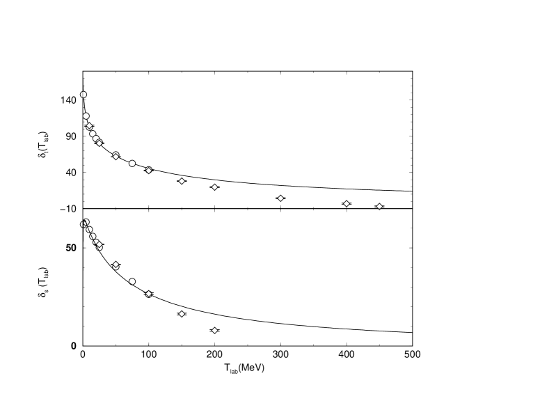
We note in conclusion that the dispersion form of the $T$-matrix for the elastic $NN$ scattering obtained for the separable interaction allows to perform analytical calculations and explicitly connect parameters of the kernel and the observables [51]. It is interesting to note that the rank I separable interaction is able to provide the low energy data even up to $T_{lab}\simeq 100$ MeV and the deuteron properties.

2.8.3 Covariant Graz-II Interaction

In the actual calculations for various electromagnetic observables, we use a more complex separable interaction, namely rank-III covariant Graz-II kernel, where partial waves with only the positive energy are taken into account (${}^{3}S_{1}^{+}$, ${}^{3}D_{1}^{+}$). In this case the functions $g_{i}$ have the following form [48],

$\displaystyle g_{1}^{{}^{3}S_{1}^{+}}(k_{0},|{\mbox{\boldmath$k$}}|)=\frac{1-\gamma_{1}(k_{0}^{2}-{\mbox{\boldmath$k$}}^{2})}{(k_{0}^{2}-{\mbox{\boldmath$k$}}^{2}-\beta_{11}^{2})^{2}},$ (179)
$\displaystyle g_{2}^{{}^{3}S_{1}^{+}}(k_{0},|{\mbox{\boldmath$k$}}|)=-\frac{(k_{0}^{2}-{\mbox{\boldmath$k$}}^{2})}{(k_{0}^{2}-{\mbox{\boldmath$k$}}^{2}-\beta_{12}^{2})^{2}},$
$\displaystyle g_{3}^{{}^{3}D_{1}^{+}}(k_{0},|{\mbox{\boldmath$k$}}|)=\frac{(k_{0}^{2}-{\mbox{\boldmath$k$}}^{2})(1-\gamma_{2}(k_{0}^{2}-{\mbox{\boldmath$k$}}^{2}))}{(k_{0}^{2}-{\mbox{\boldmath$k$}}^{2}-\beta_{21}^{2})(k_{0}^{2}-{\mbox{\boldmath$k$}}^{2}-\beta_{22}^{2})^{2}},$
$\displaystyle g_{1}^{{}^{3}D_{1}^{+}}(k_{0},|{\mbox{\boldmath$k$}}|)=g_{2}^{{}^{3}D_{1}^{+}}(k_{0},|{\mbox{\boldmath$k$}}|)=g_{3}^{{}^{3}S_{1}^{+}}(k_{0},|{\mbox{\boldmath$k$}}|)\equiv 0.$

The parameters of these functions are given in table 3.

The solution of the BS equation for the vertex function can be explicitly written as

$\displaystyle g_{{}^{3}S_{1}^{+}}(k_{0},|{\mbox{\boldmath$k$}}|)$ $\displaystyle=$ $\displaystyle(c_{1}\lambda_{11}+c_{2}\lambda_{12}+c_{3}\lambda_{13})g_{1}^{{}^{3}D_{1}^{+}}(k_{0},|{\mbox{\boldmath$k$}}|)+$
$\displaystyle(c_{1}\lambda_{12}+c_{2}\lambda_{22}+c_{3}\lambda_{23})g_{2}^{{}^{3}S_{1}^{+}}(k_{0},|{\mbox{\boldmath$k$}}|),$
$\displaystyle g_{{}^{3}D_{1}^{+}}(k_{0},|{\mbox{\boldmath$k$}}|)$ $\displaystyle=$ $\displaystyle(c_{1}\lambda_{13}+c_{2}\lambda_{23}+c_{3}\lambda_{33})g_{3}^{{}^{3}D_{1}^{+}}(k_{0},|{\mbox{\boldmath$k$}}|),$

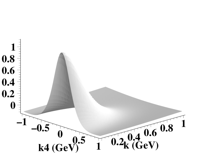
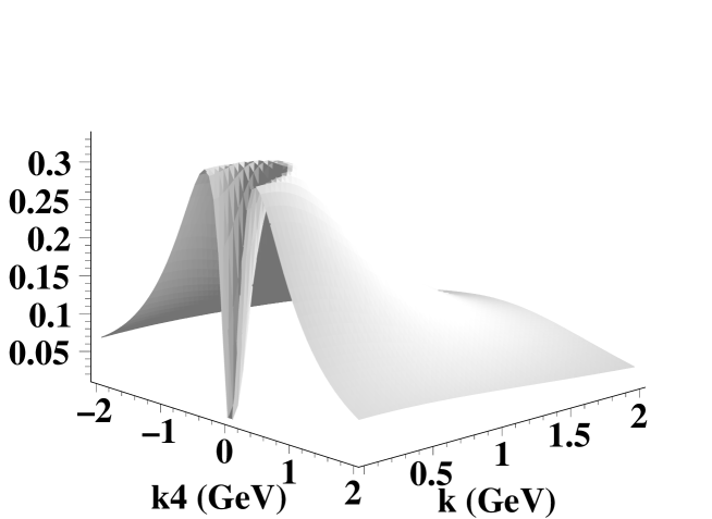
where we take into account that the matrix $\lambda$ is symmetric. Vertex functions $g_{{}^{3}S_{1}^{+}}(k_{4},|{\mbox{\boldmath$k$}}|)$ and $g_{{}^{3}D_{1}^{+}}(k_{4},|{\mbox{\boldmath$k$}}|)$ in Euclidean space ($k_{4}=ik_{0}$) are shown in Fig. 2 and Fig. 3, respectively.

To calculate the phase shifts, we use the following parametrization for on-mass-shell $T$-matrix:

$\displaystyle T(s)=-\frac{8}{\sqrt{s(s-4m^{2})}}\left(\begin{array}[]{ll}\cos{2\epsilon}\ e^{2i\delta_{\rm S}}-1&i\sin{2\epsilon}\ e^{i(\delta_{\rm S}+\delta_{\rm D})}\\ i\sin{2\epsilon}\ e^{i(\delta_{\rm S}+\delta_{\rm D})}&\cos{2\epsilon}\ e^{2i\delta_{\rm D}}-1\end{array}\right),$ (183)

where $\delta_{S}$ ($\delta_{D}$ ) are phase shifts of ${}^{3}S_{1}^{+}$- (${}^{3}D_{1}^{+}$-) waves and $\epsilon$ is the mixing parameter.

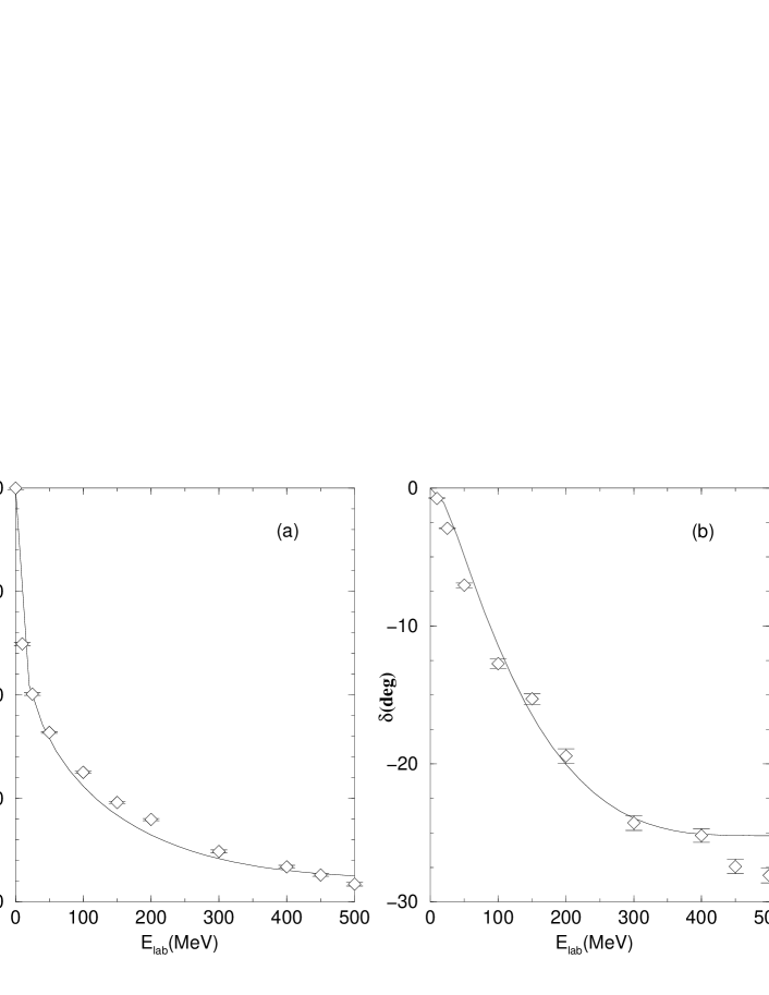
The calculated results are given in table 4 and in Fig. 4. The Bethe-Salpeter approach with the separable interaction provides the deuteron properties and also phase shifts of the nucleon-nucleon scattering in wide energy region 0–400 MeV in the $S$-$D$ chanel.

Refer to caption
Figure 2: Vertex function $g_{{}^{3}S_{1}^{+}}(k_{4},|{\mbox{\boldmath$k$}}|)$.
Refer to caption
Figure 3: Vertex function $g_{{}^{3}D_{1}^{+}}(k_{4},|\mbox{\boldmath$k$}|)$.
Table 3: Parameters of the covariant Graz-II separable interaction
$\gamma_{1}$ 28.69550 GeV-2 $\lambda_{11}$ 2.718930 $\times$ 10-4 GeV6
$\gamma_{2}$ 64.9803 GeV-2 $\lambda_{12}$ -7.16735 $\times$ 10-2 GeV4
$\beta_{11}$ 2.31384 $\times$ 10-1 GeV $\lambda_{13}$ -1.51744 $\times$ $10^{-3}$ GeV6
$\beta_{12}$ 5.21705 $\times$ $10^{-1}$ GeV $\lambda_{22}$ 16.52393 GeV2
$\beta_{21}$ 7.94907 $\times$ $10^{-1}$ GeV $\lambda_{23}$ 0.28606 GeV4
$\beta_{22}$ 1.57512 $\times$ $10^{-1}$ GeV $\lambda_{33}$ 3.48589 $\times$ $10^{-3}$ GeV6
Table 4: Properties of the deuteron and the low energy $NN$-scattering parameters in ${}^{3}S_{1}$ chanel with rank III Graz-II kernel
$p_{\rm D}(\%)$ $\epsilon_{\rm D}$ $Q_{\rm D}$ $\mu_{\rm D}$ $\rho_{\rm D/S}$ $r_{0}$ (Fm) $a$ (Fm)
(MeV) (Fm-2) ($e/2m$)
NR Graz II 4 2.225 0.2484 0.8279 0.02408 1.7861 5.4188
Cov. Graz II 4.82 2.225 0.2812 0.8522 0.0274 1.78 5.42
Exp. 2.2246 0.286 0.8574 0.0263 1.759 5.424
Refer to caption
Figure 4: (a) ${}^{3}S_{1}$- and (b) ${}^{3}D_{1}$-phase shifts calculated by using rank III Graz II kernel. Experimental data are taken from ref. [68]

2.9 Separable and One-Meson Exchange Interaction

In this section, we show the meson exchange interaction (meson-nucleon) in ladder approximation and its connection with the separable kernel with the Yamaguchi-type $g$-functions. To achieve this, we introduce simple approximation for ladder kernel:

$\displaystyle V(k_{0}^{\prime},|{\mbox{\boldmath$k$}}^{\prime}|;k_{0},|{\mbox{\boldmath$k$}}|)\to{\tilde{V}}(k_{0}^{\prime},|{\mbox{\boldmath$k$}}^{\prime}|;k_{0},|{\mbox{\boldmath$k$}}|)=\frac{V(k_{0}^{\prime},|{\mbox{\boldmath$k$}}^{\prime}|;0,0)V(0,0;k_{0},|{\mbox{\boldmath$k$}}|)}{V(0,0;0,0)}.$ (184)

Using the expressions of the kernel for scalar meson exchange ($sc$[54, 69]:

$\displaystyle V_{sc}(k_{0}^{\prime},|{\mbox{\boldmath$k$}}^{\prime}|;k_{0},|{\mbox{\boldmath$k$}}|)=-\frac{g_{sc}^{2}}{4\pi}\frac{1}{\pi^{2}}\frac{1}{4|{\mbox{\boldmath$k$}}^{\prime}||{\mbox{\boldmath$k$}}|E_{{\mbox{\boldmath$k$}}^{\prime}}E_{\mbox{\boldmath$k$}}}\left[(E_{{\mbox{\boldmath$k$}}^{\prime}}E_{\mbox{\boldmath$k$}}+m^{2})Q_{0}(z)-|{\mbox{\boldmath$k$}}^{\prime}||{\mbox{\boldmath$k$}}|Q_{1}(z)\right],$ (185)

where $z=({\mbox{\boldmath$k$}}^{\prime 2}+{\mbox{\boldmath$k$}}^{2}-(k^{\prime}_{0}-k_{0})^{2}+\mu^{2})/(2|{\mbox{\boldmath$k$}}^{\prime}||{\mbox{\boldmath$k$}}|)$, $\mu$ is the meson mass and $Q_{i}(z)$ are the Legendre functions of second kind, $Q_{0}(z)=2^{-1}\ln{(z+1)/(z-1)}$, $Q_{1}(z)=zQ_{0}(z)-1$. It can be shown that

$\displaystyle V_{sc}(k_{0}^{\prime},|{\mbox{\boldmath$k$}}^{\prime}|;0,0)=\lim_{k_{0}\to 0,|{\mbox{\boldmath$k$}}|\to 0}V_{sc}(k_{0}^{\prime},|{\mbox{\boldmath$k$}}^{\prime}|;k_{0},|{\mbox{\boldmath$k$}}|)=a_{{\mbox{\boldmath$k$}}^{\prime}}\tilde{g}(k_{0}^{\prime},|{\mbox{\boldmath$k$}}^{\prime}|),$ (186)

where

$\displaystyle a_{{\mbox{\boldmath$k$}}^{\prime}}=\frac{g_{sc}^{2}}{4\pi}\frac{1}{\pi^{2}}\frac{E_{{\mbox{\boldmath$k$}}^{\prime}}+m}{2E_{{\mbox{\boldmath$k$}}^{\prime}}},$
$\displaystyle\tilde{g}(k_{0}^{\prime},|{\mbox{\boldmath$k$}}^{\prime}|)=1/(k_{0}^{\prime 2}-{{\mbox{\boldmath$k$}}^{\prime}}^{2}-\mu^{2}).$ (187)

Expressions for $V_{sc}(0,0;k_{0},|{\mbox{\boldmath$k$}}|)$ can be obtained from Eqs. (186-187) by the following substitutions: $k_{0}^{\prime}\to k_{0}$ and $|{\mbox{\boldmath$k$}}^{\prime}|\to|{\mbox{\boldmath$k$}}|$. To make the connection between parameters, we perform $|{\mbox{\boldmath$k$}}^{\prime}|/m$-decomposition in the function $a_{{\mbox{\boldmath$k$}}^{\prime}}$ up to ${\cal O}({{\mbox{\boldmath$k$}}^{\prime}}^{2}/m^{2})$ term:

$\displaystyle a_{{\mbox{\boldmath$k$}}^{\prime}}=a_{\mbox{\boldmath$k$}}=\frac{g_{sc}^{2}}{4\pi}\frac{1}{\pi^{2}},$
$\displaystyle V_{sc}(0,0;0,0)=-\frac{g_{sc}^{2}}{4\pi}\frac{1}{\pi^{2}}\frac{1}{\mu^{2}}.$ (188)

Using the expression (184), we find:

$\displaystyle{\tilde{V}}_{sc}(k_{0}^{\prime},|{\mbox{\boldmath$k$}}^{\prime}|;k_{0},|{\mbox{\boldmath$k$}}|)=-\frac{g_{sc}^{2}}{4\pi}(\frac{\mu}{\pi})^{2}\tilde{g}(k_{0}^{\prime},|{\mbox{\boldmath$k$}}^{\prime}|)\tilde{g}(k_{0},|{\mbox{\boldmath$k$}}|).$ (189)

By comparing this expression with the separable form of kernel introduced as

$\displaystyle v(k_{0}^{\prime},|{\mbox{\boldmath$k$}}^{\prime}|,k_{0},|{\mbox{\boldmath$k$}}|;s)=\lambda g(k_{0}^{\prime},|{\mbox{\boldmath$k$}}^{\prime}|)g(k_{0},|{\mbox{\boldmath$k$}}|).$ (190)

we find the following relation between parameters:

$\displaystyle\beta=\mu,\qquad\qquad\lambda_{sc}=-\frac{g_{sc}^{2}}{4\pi}(\frac{\mu}{\pi})^{2}.$ (191)

Equations (189,191) are valid also for vector-meson-exchange kernel ($vc$) with substitution $g_{sc}\to g_{vc}$ and $\mu$ is the vector-meson mass. The separable form and can be derived from the following expression,

$\displaystyle V_{vc}(k_{0}^{\prime},|{\mbox{\boldmath$k$}}^{\prime}|;k_{0},|{\mbox{\boldmath$k$}}|)=-\frac{g_{vc}^{2}}{4\pi}\frac{1}{\pi^{2}}\frac{1}{4|{\mbox{\boldmath$k$}}^{\prime}||{\mbox{\boldmath$k$}}|E_{{\mbox{\boldmath$k$}}^{\prime}}E_{{\mbox{\boldmath$k$}}}}\left[-2(2E_{{\mbox{\boldmath$k$}}^{\prime}}E_{{\mbox{\boldmath$k$}}}+m^{2})Q_{0}(z)\right].$ (192)

For pseudoscalar-meson-exchange, the kernel of interaction has the form:

$\displaystyle V_{ps}(k_{0}^{\prime},|{\mbox{\boldmath$k$}}^{\prime}|;k_{0},|{\mbox{\boldmath$k$}}|)=-\frac{g_{sc}^{2}}{4\pi}\frac{1}{\pi^{2}}\frac{1}{4|{\mbox{\boldmath$k$}}||{\mbox{\boldmath$k$}}^{\prime}|E_{{\mbox{\boldmath$k$}}^{\prime}}E_{{\mbox{\boldmath$k$}}}}\left[-(E_{{\mbox{\boldmath$k$}}^{\prime}}E_{{\mbox{\boldmath$k$}}}-m^{2})Q_{0}(z)+|{\mbox{\boldmath$k$}}^{\prime}||{\mbox{\boldmath$k$}}|Q_{1}(z)\right],$ (193)

and for $|{\mbox{\boldmath$k$}}^{\prime}|,|{\mbox{\boldmath$k$}}|\to 0$ we can write:

$\displaystyle{\tilde{V}}_{ps}(k_{0}^{\prime},|{\mbox{\boldmath$k$}}^{\prime}|;k_{0},|{\mbox{\boldmath$k$}}|)\sim{{\mbox{\boldmath$k$}}^{\prime}}^{2}{\mbox{\boldmath$k$}}^{2}\tilde{g}(k_{0}^{\prime},|{\mbox{\boldmath$k$}}^{\prime}|)\tilde{g}(k_{0},|{\mbox{\boldmath$k$}}|).$ (194)

In the latter case ${\tilde{V}}_{ps}$ tends to zero for $|{\mbox{\boldmath$k$}}^{\prime}|,|{\mbox{\boldmath$k$}}|\to 0$, and it is impossible to find a relation between parameters similar to Eq. (191).

To illustrate the relations between parameters we used Eq. (191) and calculated values $\lambda_{\mu}$ corresponding to parameters $\mu$ and $g^{2}/4\pi$ for scalar- and vector-exchange-mesons from ref. [69]. Results are given in table 5.

Table 5: Connection between parameters of two kernels.
$J^{P}$ $\mu$ (GeV) $g^{2}/4\pi$ $\lambda$ (GeV2)
$0^{+}$ $NN\delta$ 0.983 0.64 -.06265954891
$0^{+}$ $NN\sigma^{\prime}$ 0.550 7.07 -.2166930823
$1^{-}$ $NN\rho$ 0.769 0.43 -.02576448048
$1^{-}$ $NN\omega$ 0.7826 10.6 -.6577877886

3 Elastic Electron Deuteron Scattering

The previous section was devoted to the analysis of the basic objects and methods of the BS formalism. It was shown how different dynamical processes involving bound states of particles can be included into the field-theoretical consideration. In this section, we consider the application of these methods to elastic electron scattering off the simplest bound system — the deuteron. We will highlight most important consequences which follow from the relativistic nature of the bound state.

Our interest in the electron-deuteron scattering is connected first of all with recent experimental studies of the deuteron electromagnetic forms factors in the region of high transfer momenta (see, for example, [70]-[72]), where the relativistic effects a priori play essential role, and with recent tensor polarization data [73]-[75].

Traditional nonrelativistic methods are based on the impulse approximation with allowance for relativistic corrections such as the meson-exchange currents (MEC) and retardation effects. In a number of investigations (see for example [16],[76]-[78] and references therein) it has been shown that the correct account of these effects is necessary to explain the experimental results. Generally, the deuteron elastic form factors are known to be sensitive to the choice of the strong nucleon form factor and to the MEC models. On the other hand, the recent relativistic investigations [79]-[81] show that some of the meson-exchange currents (in particular, the pair current) are automatically included in the relativistic impulse approximation.

Beside the relativistic effects, it is important to study the contribution of the nucleon form factor to the deuteron elastic form factors and to its polarization properties. There exists a number of theoretical and phenomenological models of the nucleon form factors. One finds largest differences in the results of evaluation of the electric neutron form factor $G_{\rm E}^{\rm n}(q^{2})$ as well as of the ratio $G_{\rm E}/G_{\rm M}$ for the proton at $Q^{2}=-q^{2}>$ 1 (GeV/c)2. A further progress is related with the appropriate choice of the polarization observables, which would allow the consistent analysis of the structure of the bound nucleon. In this section we apply the BS approach to the analysis of elastic electron deuteron scattering including such topics as elastic form factors and polarization tensor of the deuteron.

3.1 Relativistic Kinematics

The differential cross section for unpolarized elastic electron–deuteron scattering in the one-photon-exchange approximation (Fig. 5) is expressed in terms of the Mott cross section and deuteron structure functions $A(q^{2})$ and $B(q^{2})$ (the electron mass is neglected):

$\displaystyle\frac{d\sigma}{d\Omega_{{\rm e}}^{\prime}}=\Bigl{(}\frac{d\sigma}{d\Omega_{{\rm e}}^{\prime}}\Bigr{)}_{\rm Mott}\Bigl{[}A(q^{2})+B(q^{2})\tan^{2}{\frac{\theta_{{\rm e}}}{2}}\Bigr{]},$ (195)
$\displaystyle\Bigl{(}\frac{d\sigma}{d\Omega_{{\rm e}}^{\prime}}\Bigr{)}_{\rm Mott}=\frac{\alpha^{2}\cos^{2}{\theta_{{\rm e}}/2}}{4E_{{\rm e}}^{2}(1+2E_{{\rm e}}/M\sin^{4}{\theta_{{\rm e}}/2})},$ (196)

where $\theta_{{\rm e}}$ is the electron scattering angle, $M$ is the deuteron mass, $E_{e}$ is the incident electron energy, and

$\displaystyle A(q^{2})=F_{{\rm C}}^{2}(q^{2})+\frac{8}{9}\eta^{2}F_{\rm Q}^{2}(q^{2})+\frac{2}{3}\eta F_{\rm M}^{2}(q^{2}),$
$\displaystyle B(q^{2})=\frac{4}{3}\eta(1+\eta)F_{\rm M}^{2}(q^{2}),$ (197)

where $\eta=-{q^{2}}/{4M^{2}}=Q^{2}/4M^{2}$. The electric $F_{\rm C}(q^{2})$, the quadrupole $F_{\rm Q}(q^{2})$ and the magnetic $F_{\rm M}(q^{2})$ form factors are normalized as

$\displaystyle F_{\rm C}(0)=1,\quad F_{\rm Q}(0)=M^{2}\,Q_{\rm D},\quad F_{\rm M}(0)=\mu_{\rm D}\frac{M}{m}$ (198)

where $m$ is the nucleon mass, $Q_{\rm D}$ and $\mu_{\rm D}$ are quadrupole and magnetic moments of the deuteron, respectively. The tensor polarization components of the final deuteron are expressed through the deuteron form factors as follows:

$\displaystyle T_{20}\ \bigl{[}A+B\tan^{2}{\frac{\theta_{{\rm e}}}{2}}\bigr{]}=-\frac{1}{\sqrt{2}}\bigl{[}\frac{8}{3}\eta F_{\rm C}F_{\rm Q}+\frac{8}{9}\eta^{2}F_{\rm Q}^{2}+\frac{1}{3}\eta(1+2(1+\eta)\tan^{2}{\frac{\theta_{{\rm e}}}{2}})F_{\rm M}^{2}\bigr{]},$
$\displaystyle T_{21}\ \bigl{[}A+B\tan^{2}{\frac{\theta_{{\rm e}}}{2}}\bigr{]}=\frac{2}{\sqrt{3}}\eta(\eta+\eta^{2}\sin^{2}{\frac{\theta_{{\rm e}}}{2}})^{1/2}F_{\rm M}F_{\rm Q}\sec{\frac{\theta_{{\rm e}}}{2}},$ (199)
$\displaystyle T_{22}\ \bigl{[}A+B\tan^{2}{\frac{\theta_{{\rm e}}}{2}}\bigr{]}=-\frac{1}{2\sqrt{3}}\eta F_{\rm M}^{2}.$

Equation (195) can be obtained by using the standard technique [42] from the following amplitude of the process

$\displaystyle M_{\rm fi}=ie^{2}{\bar{u}_{m^{\prime}}(l^{\prime})}\gamma^{\mu}u_{m}(l)\;\frac{1}{q^{2}}\;\langle D^{\prime}{\cal M}^{\prime}|J_{\mu}|D{\cal M}\rangle,$ (200)

where $u_{m}(l)$ denotes the free electron spinor with 4-momentum $l$ and spin projection $m$, and $q=l-l^{\prime}=P^{\prime}-P$ is the 4-momentum transfer, $P(P^{\prime})$ is the initial (final) deuteron momentum; $|D{\cal M}\rangle$ is the deuteron state with total angular momenta projection ${\cal M}$, and $J_{\mu}$ is the electromagnetic current operator.

[Uncaptioned image]
Figure 5: Electron-deuteron elastic scattering in the one-photon approximation.

The deuteron current matrix element is usually parameterized in the following way (due to $P$- and $T$-parity conservation and gauge invariance):

$\displaystyle\langle D^{\prime}{\cal M}^{\prime}|J_{\mu}|D{\cal M}\rangle=$ $\displaystyle-$ $\displaystyle e\;\xi^{*}_{\alpha\;{\cal M}^{\prime}}(P^{\prime})\;\xi_{\beta\;{\cal M}}(P)\;\Biggl{[}(P^{\prime}+P)_{\mu}\Bigl{(}g^{\alpha\beta}F_{1}(q^{2})-\frac{q^{\alpha}q^{\beta}}{2M^{2}}F_{2}(q^{2})\Bigr{)}$ (201)
$\displaystyle-$ $\displaystyle(q^{\alpha}g^{\beta}_{\mu}-q^{\beta}g^{\alpha}_{\mu})G_{1}(q^{2})\Biggr{]},$

where $\xi_{\cal M}(P)$ and $\xi^{*}_{{\cal M}^{\prime}}(P^{\prime})$ are the polarization 4-vectors of the initial and final deuteron, respectively. Form factors $F_{1,2}(q^{2})$, $G_{1}(q^{2})$ are related to $F_{\rm C}(q^{2})$, $F_{\rm Q}(q^{2})$ and $F_{\rm M}(q^{2})$ by the equations

$\displaystyle F_{\rm C}=F_{1}+\frac{2}{3}\eta\bigl{[}F_{1}+(1+\eta)F_{2}-G_{1}\bigr{]},\quad F_{\rm Q}=F_{1}+(1+\eta)F_{2}-G_{1},\quad F_{\rm M}=G_{1}.$ (202)

The normalization condition for the deuteron current matrix element has the form (in contrast to (38) $i$ is included into the matrix element):

$\displaystyle\lim_{q^{2}\to 0}\langle D^{\prime}{\cal M}^{\prime}|J_{\mu}|D{\cal M}\rangle=2eP_{\mu}\;\delta_{{\cal M}{\cal M}^{\prime}}~{}.$

To calculate the deuteron form factors one should use the particular system of reference. In the laboratory frame the 4-vectors have the following form (the $Z$–axis is along the photon momentum):

$\displaystyle P=(M,{\bf 0}),\quad P^{\prime}=(M(1+2\eta),0,0,2M\sqrt{\eta}\sqrt{1+\eta}),$
$\displaystyle q=(2M\eta,0,0,2M\sqrt{\eta}\sqrt{1+\eta}),$ (203)
$\displaystyle\xi_{{\cal M}=+1}(P)=\xi_{{\cal M}=+1}(P^{\prime})=-\frac{1}{\sqrt{2}}(0,1,i,0),$
$\displaystyle\xi_{{\cal M}=-1}(P)=\xi_{{\cal M}=-1}(P^{\prime})=\frac{1}{\sqrt{2}}(0,1,-i,0),$
$\displaystyle\xi_{{\cal M}=0}(P)=(0,0,0,1),\quad\xi_{{\cal M}=0}(P^{\prime})=(2\sqrt{\eta}\sqrt{1+\eta},0,0,1+2\eta).$ (204)

Using expressions (203,204) and the parameterization in the form of Eq. (201) one obtains:

$\displaystyle\langle{\cal M}^{\prime}|J_{0}|{\cal M}\rangle=\;2Me\;(1+\eta)\;\Bigl{\{}F_{1}\delta_{{\cal M}{\cal M}^{\prime}}+2\eta\bigl{[}F_{1}+(1+\eta)F_{2}-G_{1}\bigr{]}\delta_{{\cal M}^{\prime}0}\delta_{{\cal M}0}\Bigr{\}},$
$\displaystyle\langle{\cal M}^{\prime}|J_{x}|{\cal M}\rangle=\;\frac{2Me}{\sqrt{2}}\;\sqrt{\eta}\;\sqrt{1+\eta}\;G_{1}\;\Bigl{\{}\delta_{{\cal M}^{\prime}{\cal M}+1}-\delta_{{\cal M}^{\prime}{\cal M}-1}\Bigr{\}}.$ (205)

To calculate the deuteron form factors, one should know three matrix elements with different total angular momentum projections and current components.

3.2 Gauge Invariance and Gauge Independence in the Bethe–Salpeter Approach

It is well known that the principle of gauge invariance imposes stringent constraints on the amplitudes of electromagnetic interactions with bound systems. In the first order of perturbation theory in the charge $e$, this principle leads to the continuity equation for the electromagnetic-current-density operator and to the Ward-Takahashi (WT) identity for the five-point Green’s function. We will consider the WT identity for the five-point Green’s function and its implications for the Mandelstam current, which determines the amplitude of electron scattering on deuterons in the Bethe Salpeter formalism.

The continuity equations for the bare (Noether) current and effective currents (for example, the Mandelstam current or conserved currents in nonrelativistic quantum mechanics) are not sufficient for ensuring the gauge invariance of the amplitudes of electromagnetic transitions  [82]-[86]. Moreover, both initial and final states must correspond to the current used in the analysis.

As a rule, the conserved deuteron electromagnetic current includes two-particle contributions associated with meson-exchange currents or interaction currents. At the same time, it was shown in [48, 85, 86], that the amplitude of elastic $e{\rm D}$ scattering can be gauge invariant in the relativistic impulse approximation, which is based on the concept of the one-particle scattering mechanism. This result was obtained in the BS formalism with one boson exchange (OBE) potentials and with separable interactions. At first glance, it is at odds with the common point of view on the problem of gauge invariance [84].

Our objective here is to study in detail the conditions under which the gauge-invariant description of elastic electron scattering can be achieved in other models for constituent interaction. In addition, we discuss a certain extension of the WT identity [87, 88] for an arbitrary system of charged particles.

For a two-fermion system, the Mandelstam current can be represented as

$\displaystyle J_{\mu}=J^{(1)}_{\mu}+J^{(2)}_{\mu},$ (206)

where $J^{(1)}_{\mu}\equiv J^{RIA}_{\mu}$ and $J^{(2)}_{\mu}$, are, respectively, the one-particle, and two-particle contributions that satisfy the relations [82]

$\displaystyle iq^{\mu}$ $\displaystyle J^{(RIA)}_{\mu}(k^{\prime},k;P^{\prime},P)=e_{1}\delta(k^{\prime}-k-q/2)\left[S^{(1)}(P/2+k)^{-1}-S^{(1)}(P^{\prime}/2+k^{\prime})^{-1}\right]S^{(2)}(P/2-k)^{-1}+$ (207)
$\displaystyle+$ $\displaystyle e_{2}\delta(k^{\prime}-k+q/2)\left[S^{(2)}(P/2-k)^{-1}-S^{(2)}(P^{\prime}/2-k^{\prime})^{-1}\right]S^{(1)}(P/2+k)^{-1},$
$\displaystyle iq^{\mu}$ $\displaystyle J^{(2)}_{\mu}(k^{\prime},k;P^{\prime},P)=e_{1}V(P,k^{\prime}-q/2,k)-V(P^{\prime},k^{\prime},k+q/2;)e_{1}+$ (208)
$\displaystyle+$ $\displaystyle e_{2}V(P,k^{\prime}+q/2,k)-V(P^{\prime},k^{\prime},k-q/2)e_{2}.$

Here, $k$ and $P$ ($k^{\prime}$ and $P^{\prime}$) are the relative and total 4-momenta in the initial (final) states, respectively; $q=(\omega,\vec{q})$ is the 4-momentum transfer; $P^{\prime}=P+q$; $S^{(1,2)}(k)$ is the dressed nucleon propagator; and $V(P,k^{\prime},k)$ is the kernel of the BS equation. This kernel depends on the relative momenta $k$ and $k^{\prime}$ and on the total momentum $P$. In the isospin formalism, we have

$\displaystyle e_{i}=|e|\frac{1+\tau_{z}(i)}{2}$ (209)

where $e$ is an electron charge, and $\tau_{z}(i)$ are the Pauli matrices (i = 1, 2).

It is worth noting that equations (207) and (208) do not define the current completely. They only impose certain constraints on the longitudinal component of the current.

The amplitude of elastic $e{\rm D}$ scattering can be represented in the form (see (200))

$$M^{J}_{M^{\prime}M}=\epsilon^{\mu}\int\frac{d^{4}k}{(2\pi)^{4}}\frac{d^{4}k^{\prime}}{(2\pi)^{4}}\bar{\Phi}^{JM^{\prime}}(P^{\prime},k^{\prime})J_{\mu}(k^{\prime},k,P^{\prime},P)\Phi^{JM}(P,k)\equiv\epsilon^{\mu}({\cal M}^{J}_{M^{\prime}M})_{\mu},$$ (210)

where $\Phi^{JM}(P,k)$ ($\Phi^{JM^{\prime}}(P^{\prime},k^{\prime})$) (66) is the BS amplitude, which describes the initial (final) state, and $\epsilon^{\mu}$ is the virtual-photon polarization vector. The gauge-independence condition

$$q^{\mu}({\cal M}^{J}_{M^{\prime}M})_{\mu}=q^{\mu}[({\cal M}^{J}_{M^{\prime}M})_{\mu}^{RIA}+({\cal M}^{J}_{M^{\prime}M})_{\mu}^{(2)}]=0$$ (211)

is met if the current satisfies identities (207) and (208) and if the amplitudes $\Phi^{JM}(P,k)$ and $\Phi^{JM^{\prime}}(P^{\prime},k^{\prime})$ satisfy the BS equation with the same kernel (51).

In the relativistic impulse approximation illustrated in Fig. 6, the deuteron matrix element ${\cal M}^{RIA}$, defined by the Eq.(211), for on-shell $\gamma NN$ vertex satisfies the gauge-independence condition [91]

$$q^{\mu}({\cal M}^{J}_{M^{\prime}M})_{\mu}^{RIA}=0.$$ (212)

It implies that

$$q^{\mu}({\cal M}^{J}_{M^{\prime}M})_{\mu}^{(2)}=\int\frac{d^{4}k}{(2\pi)^{4}}\frac{d^{4}k^{\prime}}{(2\pi)^{4}}\bar{\Phi}^{JM^{\prime}}(P^{\prime},k^{\prime})J^{(2)}_{\mu}(k^{\prime},k,P^{\prime},P)\Phi^{JM}(P,k)=0.$$ (213)

It turns out that, for certain models of interaction, this relation holds. Let us isolate isospin structure in $V$. We have

$$V(P,k^{\prime},k)=\sum\limits_{T=0,1}\Pi_{T}V_{T}(P,k^{\prime},k),$$ (214)

where $\Pi_{T}$ is the projection operator onto the state with total isospin $T$, and $V_{T}$ is the corresponding component of interaction. In the ladder approximation,

$$V_{T}(P,k^{\prime},k)={\cal V}_{T}(k^{\prime}-k),$$ (215)

we can verify that the condition (213) is satisfied for any function ${\cal V}_{T}(k^{\prime}-k)$. This result is independent of the isospin value in the initial or final state, although only one ${\cal V}_{0}(k^{\prime}-k)$ component contributes to (213) in the case of $eD$-scattering. We note that all OBE interactions can be represented in the form (215) and that the corresponding amplitudes are gauge independent, in accord with the result reported in [85, 86].

As the next example, we consider the interaction described by a separable potential (125). The authors of [48, 90] proved that the amplitude in the impulse approximation is a gauge-independent quantity in this case. Their proof is based on the transformation properties of the quantities in Eq.(213) under boosts.

However, this result can be obtained in a simpler way by calculating the contraction in (211) and by considering that, for interaction of the form (125), the BS amplitude in (213) is independent of the total momentum $P$ (see [91]).

Thus, we can conclude that, in the ladder and separable approximations for the kernel of the BS equation, the amplitude of elastic scattering in the impulse approximation is gauge independent. The common feature of the kernels in this section is that they are independent of the total momentum of the pair.

These conclusions do not mean that other gauge-independent contribution can always be disregarded (for example, the contribution of the exchange currents). Indeed, the results reported in [92, 93], where the $q\bar{q}$ system with separable interaction was studied, revealed that two-particle currents exert a noticeable effect on the pion charge form factor, especially at high momentum transfers. We can state with confidence that, for a certain model of $NN$ interaction, two-particle and more complicated electromagnetic currents must be taken into account in a consistent manner even in calculating the elastic nuclear form factors. However, there is no universal recipe for constructing these currents for a given interaction of particles in a bound system.

3.3 Relativistic Impulse Approximation

In the relativistic impulse approximation illustrated in Fig. 6, the deuteron current matrix element can be written as

$\displaystyle\langle D^{\prime}{\cal M}^{\prime}|J^{RIA}_{\mu}|D{\cal M}\rangle=ie\int\frac{d^{4}k}{(2\pi)^{4}}{\rm Tr}\biggl{\{}{\bar{\chi}^{{}_{1{\cal M}^{\prime}}}}(P^{\prime},k^{\prime})\Gamma^{\rm(S)}_{\mu}(q)\chi^{{}_{1{\cal M}}}(P,k)({P\cdot\gamma}/{2}-{k\cdot\gamma}+m)\biggr{\}},$ (216)

where $\chi^{{}_{1{\cal M}}}(P,k)$ is the BS amplitude of the deuteron, $P^{\prime}=P+q$ and $k^{\prime}=k+q/2$. The vertex of $\gamma NN$ interaction,

$\displaystyle\Gamma_{\mu}^{\rm(S)}(q)=\gamma_{\mu}F_{1}^{\rm(S)}(q^{2})-\frac{\gamma_{\mu}{q\cdot\gamma}-{q\cdot\gamma}\gamma_{\mu}}{4m}F_{2}^{\rm(S)}(q^{2}),$ (217)

is chosen to be the form factor on mass shell. The isoscalar form factors of the nucleon $F_{1,2}^{\rm(S)}(q^{2})=(F_{1,2}^{\rm(p)}(q^{2})+F_{1,2}^{\rm(n)}(q^{2}))/2$, which appeared due to the summation of two nucleons, are normalized as $F_{1}^{\rm(S)}(0)=1/2$ and $F_{2}^{\rm(S)}(0)=(\varkappa_{p}+\varkappa_{n})/2$ with $\varkappa_{p}=\mu_{p}-1$ and $\varkappa_{n}=\mu_{n}$ being anomalous parts of the proton ($\mu_{p}$) and neutron ($\mu_{n}$) magnetic moments, respectively.

[Uncaptioned image]
Figure 6: Relativistic impulse approximation for the elastic electron deuteron scattering.

It should be noted that the choice of the $\gamma NN$ vertex in a form (217) and disregard the current interaction (CI) (two-nucleon currents), in general, breaks the gauge independence of the reaction. Nevertheless, as it was shown in [91], there exist two cases when RIA and CI are gauge independent separately. The first case corresponds to the separable interaction with no dependence on the total momentum in the radial functions, and the second one to the one-meson exchange kernel.

First, the trace was taken in Eq. (216). The covariant form for the BS amplitude (2.6.2) was used. After taking the trace, the scalar products of 4-momenta ($P,k,q$) and the deuteron polarization 4-vectors ($\xi_{\cal M},\xi^{*}_{{\cal M}^{\prime}}$) with definite spin projections were inserted. Then, using Eqs. (2.6.2), functions $h_{i}$ were expressed in terms of functions $\phi_{JLS\varrho}$ (see section 2.6.2). All scalar products were evaluated in the laboratory frame.

The resulting expressions for the deuteron current matrix element can be written as

$\displaystyle\langle D^{\prime}{\cal M}^{\prime}|J^{RIA}_{\mu}|D{\cal M}\rangle={\cal I}_{1\;\mu}^{{\cal M}^{\prime}{\cal M}}(q^{2})\;F_{1}^{\rm(S)}(q^{2})+{\cal I}_{2\;\mu}^{{\cal M}^{\prime}{\cal M}}(q^{2})\;F_{2}^{\rm(S)}(q^{2}),$ (218)
$\displaystyle{\cal I}_{1,2\;\mu}^{{\cal M}^{\prime}{\cal M}}(q^{2})=ie\int dk_{0}\;|{\mbox{\boldmath$k$}}|^{2}\;d|{\mbox{\boldmath$k$}}|\;d(\cos{\theta})\sum_{L^{\prime}S^{\prime}\varrho^{\prime},LS\varrho}\phi_{{}_{1L^{\prime}S^{\prime}\varrho}}(k_{0}^{\prime},|{\mbox{\boldmath$k$}}^{\prime}|)\phi_{{}_{1LS\varrho}}(k_{0},|{\mbox{\boldmath$k$}}|)\;I^{L^{\prime},L}_{1,2\;{\cal M^{\prime}}{\cal M}\;\mu}(k_{0},|{\mbox{\boldmath$k$}}|,\cos{\theta},q^{2}),$

where the function $I^{L^{\prime},L}_{1,2\;{\cal M^{\prime}}{\cal M}\;\mu}(k_{0},|{\mbox{\boldmath$k$}}|,\cos{\theta},q^{2})$ is a result of the trace calculation and the substitution of the scalar products into Eq. (216).

In Eq. (218), the radial part of the BS amplitude for the final deuteron $\phi_{1L^{\prime}S^{\prime}\varrho^{\prime}}(k_{0}^{\prime},|{\mbox{\boldmath$k$}}^{\prime}|)$ depends on the components of the 4-vector $k^{\prime}$ calculated in the rest frame ($rf$). The vectors in the rest frame and in the laboratory frame are related via Lorentz transformation:

$\displaystyle P^{\prime}_{lab}={\cal L}P^{\prime}_{rf}={\cal L}(M,{\bf 0}),\quad k^{\prime}_{lab}={\cal L}k^{\prime}_{rf},$ (219)

where the Lorentz transformation matrix ${\cal L}$ is of the form:

$\displaystyle{\cal L}=\left(\begin{array}[]{cccc}1+2\eta&0&0&2\sqrt{\eta}\sqrt{1+\eta}\\ 0&1&0&0\\ 0&0&1&0\\ 2\sqrt{\eta}\sqrt{1+\eta}&0&0&1+2\eta\end{array}\right)$ (224)

To simplify the notations, the components of the 4-vector $k^{\prime}_{rf}$ are denoted by $k^{\prime}\equiv k^{\prime}_{rf}=(k_{0}^{\prime},k_{x}^{\prime},k_{y}^{\prime},k_{z}^{\prime})$, and $|{{\mbox{\boldmath$k$}}}^{\prime}|=|{{\mbox{\boldmath$k$}}}^{\prime}_{rf}|=\sqrt{k_{x}^{\prime\,2}+k_{y}^{\prime\,2}+k_{z}^{\prime\,2}}$. Using relations (203), (219) and (224) one finds

$\displaystyle k_{0}^{\prime}$ $\displaystyle=$ $\displaystyle(1+2\eta)k_{0}-2\sqrt{\eta}\sqrt{1+\eta}k_{z}-M\eta,$
$\displaystyle k_{x}^{\prime}$ $\displaystyle=$ $\displaystyle k_{x},\quad k_{y}^{\prime}=k_{y},$
$\displaystyle k_{z}^{\prime}$ $\displaystyle=$ $\displaystyle(1+2\eta)k_{z}-2\sqrt{\eta}\sqrt{1+\eta}k_{0}+M\sqrt{\eta}\sqrt{1+\eta},$ (225)

where $k_{0},k_{x},k_{y},k_{z}$ are the components of the 4-vector $k$ in the deuteron rest frame.

3.4 Numerical Results

The calculations were performed with a covariant separable kernel of $NN$-interaction Graz II (for details, see section 2.8.3). Considering only ${}^{3}S_{1}^{+}$ and ${}^{3}D_{1}^{+}$ states one writes (see Eq. (76))

$$\phi_{{}_{1LS+}}(k_{0},|{\mbox{\boldmath$k$}}|)=S_{+}(k_{0},|{\mbox{\boldmath$k$}}|;s)g_{{}_{1LS+}}(k_{0},|{\mbox{\boldmath$k$}}|),$$

where $g_{{}_{1LS+}}$ is the radial part of the vertex function. Thus, the Bethe-Salpeter amplitude involves singularities in the $k_{0}$ plane, which are infinitesimally close to the real axis. Some of the singularities arise from the propagator, while the others come from the radial part of the vertex function — in other words, from the functions $g_{i}^{1LS+}$ defined in Eqs. (179).

For the initial deuteron, the singularities do not depend on $q^{2}$ (or $\eta$) and always remain in the same quadrant:

$\displaystyle\mbox{for the propagator}\qquad\quad k_{0}=\pm M/2\mp\sqrt{{\mbox{\boldmath$k$}}^{2}+m^{2}}\pm i\epsilon,$
$\displaystyle\mbox{for the functions $g_{i}^{1LS+}$}\quad\quad k_{0}=\pm\sqrt{{\mbox{\boldmath$k$}}^{2}+\beta_{i}^{2}}\mp i\epsilon.$

The situation changes for the final deuteron. Due to the boost of the arguments (225) of the amplitude, the singularities depend on $q^{2}$ (or $\eta$) and can go across the imaginary axis and appear in another quadrant (mobile singularities). The positions of the singularities are the following:

for the propagator
$\displaystyle\hskip 14.22636ptk_{0}=-(1+4\eta)M\pm\sqrt{{\mbox{\boldmath$k$}}^{2}+m^{2}+4\sqrt{\eta(1+\eta)}M|{\mbox{\boldmath$k$}}|\cos{\theta}+4\eta^{2}(1+\eta)^{2}M^{2}}\pm i\epsilon,$
for the functions $g_{i}^{(L)}$
$\displaystyle\hskip 14.22636ptk_{0}=-\eta M\pm\sqrt{{\mbox{\boldmath$k$}}^{2}+\beta_{i}^{2}+2\sqrt{\eta(1+\eta)}M|{\mbox{\boldmath$k$}}|\cos{\theta}+\eta^{2}(1+\eta)^{2}M^{2}}\mp i\epsilon.$

The mobility of the singularities does not affect the calculations if the Cauchy theorem is applied. But for the Wick rotation procedure, this means that the additional contributions (the residues at these mobile singularities) should be taken into account. The minimal value of $-q^{2}$ for which the imaginary axis is traversed is: for propagator $-q^{2}=M(2m-M)\approx 4.17\times 10^{-3}$ (GeV/c)2, for $g_{i}^{1LS+}$ functions $-q^{2}=4M\beta_{i}\approx 1.17$ (GeV$/c)^{2}$. The contributions of the residues from the functions $g_{i}^{1LS+}$ are negligible (about $1\%$) in the region $-q^{2}<2$ (GeV/c)2, and are getting larger with growing momentum transfer. But the contribution of the residue from the propagator is very large and can modify the curves significantly even in the region $-q^{2}<2$ (GeV/c)2.

The contribution of the residue from the propagator is shown in Fig. 7 for the functions $A(q^{2})$ and $B(q^{2})$. The contribution is substantially large both for the function $A(q^{2})$ and the function $B(q^{2})$ (for the function $B(q^{2})$, this contribution fills the minimum, which does not exist in the experimental data). This result can be considered as a specific relativistic effect caused by the Lorentz transformation in the arguments of the Bethe-Salpeter amplitude (vertex functions and propagator). The comparison of the relativistic (RIA) and the nonrelativistic (NRIA) calculations with the separable kernel of the $NN$-interaction Graz II is shown in Fig. 9, also. One can see that the difference between the RIA and the NRIA calculations rather small. However we must keep in mind that the RIA calculations does not include the contribution of the $P$-waves to the deuteron (further development of the RIA calculations must take into account this contribution) and the NRIA calculations does not take into account the mesonic exchange currents. Only after that we can draw the conclusion about the full contribution of the relativistic effects to the structure functions of the deuteron.

Yet another interesting result of the investigations is the dependence of the deuteron form factors on the nucleon form factors — in particular, on the neutron electric form factor $G_{\rm E}^{\rm n}(q^{2})$. The electric and the magnetic form factors of nucleons ($G_{\rm E}(q^{2})$ and $G_{\rm M}(q^{2})$, respectively) are related to the Dirac and Pauli form factors ($F_{1}(q^{2})$ and $F_{2}(q^{2})$, respectively) by the equations

$\displaystyle G_{\rm E}(q^{2})$ $\displaystyle=$ $\displaystyle F_{1}(q^{2})+\frac{q^{2}}{4m^{2}}F_{2}(q^{2}),$
$\displaystyle G_{\rm M}(q^{2})$ $\displaystyle=$ $\displaystyle F_{1}(q^{2})+F_{2}(q^{2}).$ (226)

Three sets of the nucleon form factors are used in the calculations. The first set is so-called dipole fit

$\displaystyle G_{\rm M}^{\rm p}(q^{2})=(1+\kappa_{\rm p})G_{\rm E}^{\rm p}(q^{2}),\qquad G_{\rm M}^{\rm n}=\kappa_{\rm n}G_{\rm E}^{\rm p}(q^{2}),\qquad G_{\rm E}^{\rm n}(q^{2})=0,$
$\displaystyle G_{\rm E}^{\rm p}(q^{2})=1/(1-q^{2}/0.71{\mbox{(}{\rm GeV}/c)}^{2})^{2},$ (227)

where $\kappa_{\rm p}=1.7928$, $\kappa_{\rm n}=-1.9130$ are the anomalous magnetic moments of the nucleons. The second set was suggested by the vector meson dominance model (VMDM) [94]

$\displaystyle F_{1}^{(\rm S)}(t)=\left[\frac{m_{\omega}^{2}}{m_{\omega}^{2}-q^{2}}\gamma_{\omega}+(1-\gamma_{\omega})\right]F_{1L},$ (228)
$\displaystyle F_{2}^{(\rm S)}(t)=\left[\frac{m_{\omega}^{2}}{m_{\omega}^{2}-q^{2}}\kappa_{\omega}\gamma_{\omega}+(1+\kappa_{p}+\kappa_{n}-\kappa_{\omega}\gamma_{\omega})\right]F_{2L},$
$\displaystyle F_{1L}=\frac{\lambda_{1}^{2}}{\lambda_{1}^{2}+{\hat{q}}^{2}}\frac{\lambda_{2}^{2}}{\lambda_{2}^{2}+{\hat{q}}^{2}},\qquad F_{2L}=\frac{\lambda_{1}^{2}}{\lambda_{1}^{2}+{\hat{q}}^{2}}\left(\frac{\lambda_{2}^{2}}{\lambda_{2}^{2}+{\hat{q}}^{2}}\right)^{2},$
$\displaystyle{\hat{q}}^{2}\,=\,-q^{2}\,\frac{\ln{(\lambda_{2}^{2}-q^{2})/\lambda_{3}^{2}}}{\ln{\lambda_{2}^{2}/\lambda_{3}^{2}}},$

where $\lambda_{1}=0.795$ (GeV/c), $\lambda_{2}=2.27$ (GeV/c), $\lambda_{3}=0.29$ (GeV/c), $\kappa_{\omega}=0.163$, $\gamma_{\omega}=0.411$, $m_{\omega}=0.784$ (GeV/c). The third set is that from relativistic harmonic oscillator model (RHOM) [95]

$\displaystyle G_{\rm E}^{\rm p}=I^{(3)}(q^{2}),$ (229)
$\displaystyle G_{\rm E}^{\rm n}=-\frac{q^{2}}{2m^{2}}I^{(3)}(q^{2}),$
$\displaystyle\frac{G_{\rm M}^{\rm p}(q^{2})}{1+\kappa_{p}}=\frac{G_{\rm M}^{\rm n}(q^{2})}{\kappa_{n}}=I^{(3)}(q^{2}),$
$\displaystyle I^{(3)}(q^{2})=\frac{1}{(1-q^{2}/2m^{2})^{2}}\,{\rm exp}\left(\frac{1}{2\alpha_{3}}\ \frac{q^{2}}{1-q^{2}/2m^{2}}\right),\qquad\qquad\alpha_{3}=0.42({\rm GeV}/c)^{2}.$

The first model assumes that the neutron electric form factor is equal to zero. Two other models lead to a nonzero $G_{\rm E}^{\rm n}$.

Figure 8 shows the charge and quadrupole form factors ($F_{\rm C}(q^{2})$ and $F_{\rm Q}(q^{2})$, respectively). The zero of the form factor $F_{\rm C}(q^{2})$ is in the range of $-q^{2}=1.2-1.35$ (GeV/$c$)2, but experimental data yield $-q^{2}=0.69-0.83$ (GeV/$c$)2 [73]-[75]. This dip comes from the specific choice of the separable Graz II kernel (in the calculations with non-relativistic Graz II potential, the zero of $F_{\rm C}(q^{2})$ is shifted too). The nucleon form factors do not shift the zero in the form factor $F_{\rm C}(q^{2})$. The nucleon form factors with the nonzero electric from factor for the neutron (VMDM and RHOM) are more suitable for the description of the experimental data on the quadrupole form factor $F_{\rm Q}(q^{2})$. We stress that the contriburion of the $P$-waves (the negative energy states of the BS amplitude) for the deuteron must shift the dip of the $F_{C}(Q^{2})$ and must give better agreement with the experimental data analogously the NRIA calculations with the taking into account of the mesonic exchange currents [16]. The structure functions $A(q^{2})$ and $B(q^{2})$ are shown in Fig. 9. The RIA calculations of the structure functions of the deuteron show the strong dependence on choice the form factors of the nucleon. After taking into account the contribution of the $P$-waves for the deuteron we can make more exact conclusion about the choice of the nucleon form factors. Figures 10 and 11a show the tensor polarization components $T_{20}(q^{2}),T_{21}(q^{2})$ and $T_{22}(q^{2})$ for the final deuteron calculated with $\theta_{e}=70^{\circ}$. It is seen that $T_{20}(q^{2})$ and $T_{22}(q^{2})$ have very weak dependence on the nucleon form factors, but for $T_{21}(q^{2})$ it is more pronounced. The $T_{21}(q^{2})$ calculated with three different electron scattering angles $\theta_{e}=19.8^{\circ},\ 70^{\circ},\ 80.9^{\circ}$ is shown in the Fig. 11b. The change in the electron scattering angle affects sizably the component $T_{21}(q^{2})$. Figure 11c shows the result of calculation of the component $T_{21}(q^{2})$ with different nucleon form factors at electron scattering angles fixed in experiment. This result can be used to choose between the models for the nucleon form factors. Unfortunately, large uncertainties in experimental data prevent from choosing between the sets, and future measurements of the component $T_{21}(q^{2})$ can be very useful for the analysis.

Note that the calculated $T_{20}(q^{2})$ differs from the experimental data in the region $-q^{2}>0.6$ (GeV/c)2. This fact, apparently, could be explained by several reasons. It is necessary to improve the description of the zero of the charge form factor $F_{\rm C}(q^{2})$ by changing the separable kernel of $NN$-interaction and taking into account the negative energy states of the Bethe-Salpeter amplitude for the deuteron. It is also important to investigate the contribution of the two-body electromagnetic current. Information about the effect of these factors provide a powerful tool in the study of the on- and off-shell behavior of the nucleon form factors in elastic electron deuteron scattering.

Figure 7: (a) Structure function $A(q^{2})$. Long dashes represent the calculation without the contribution of mobile singularities (no mobile singularities - NMS). The solid curve shows the full relativistic impulse approximation calculation. Short dashes correspond to the nonrelativistic impulse approximation calculation (nonrelativistic Graz II potential). Experimental data are taken from [96]-[98],[70, 71]. (b) Structure function $B(q^{2})$. Notations for the curves are identical to those of Fig. 7a. Experimental data are taken from [96, 99, 100, 101, 72].
Figure 8: (a) Charge form factor $F_{\rm C}(q^{2})$. Long and short dashes represent calculations with the VMDM and RHOM nucleon form factors, respectively. The solid curve corresponds to the dipole fit. The experimental data are taken from ref. [75]. (b) Quadrupole form factor $F_{\rm Q}(q^{2})$. Notations for the curves are identical to those of Fig. 8a, and the experimental data originate from the same source.
Figure 9: (a) Deuteron structure function $A(q^{2})$. Notations for the curves are identical to those of Fig. 8a. Experimental data originate from the same source as in Fig. 7a. (b) Deuteron structure function $B(q^{2})$. Notations for the curves are identical to those of Fig. 8b. The experimental data originate from the same source as in Fig. 7b.
Figure 10: (a) Tensor polarization component $T_{20}(q^{2})$ calculated at $\theta_{e}=70^{\circ}$. Notations for the curves are identical to those of Fig. 8a. Experimental data are taken from ref. [75] (values from  [73, 74],[102]-[108] were recalculated at $\theta_{e}=70^{\circ}$). (b) Tensor polarization components $T_{22}(q^{2})$ calculated at $\theta_{e}=70^{\circ}$. Notations for the curves are identical to those of Fig. 8a. Experimental data are taken from ref. [73, 74].

Figure 11: (a) Tensor polarization component $T_{21}(q^{2})$ calculated at $\theta_{e}=70^{\circ}$. Notations for the curves are identical to those of Fig. 8a. Experimental data originate from the same source as in Fig. 8b. (b) Tensor polarization component $T_{21}(q^{2})$ calculated at different angles $\theta_{{\rm e}}=19.8^{\circ},70^{\circ},80.9^{\circ}$ (solid curve, long and short dashes, respectively) with dipole nucleon form factor. The data points are from the same source as in Fig. 11b. (c) Tensor polarization component $T_{21}(q^{2})$ calculated with dipole fit ($\nabla$), VMDM ($\circ$) and RHOM ($\diamond$) at experimental electron scattering angle values. The data points originate from the same source as in Fig. 10b.

3.5 Electromagnetic Moments of the Deuteron

In the previous section, the electromagnetic form factors of the deuteron were discussed. The relativistic effects in the form factors were analyzed in detail. The sensitivity of the polarization observables to the models for the nucleon form factors was discussed too.

Now we consider static electromagnetic characteristics of the deuteron — magnetic and quadrupole moments — in details. As it was shown in ref. [109], the relativistic effects in BS approach, such as effects of relativistic kinematics, retardation effects or negative energy states, play essential role in evaluation of static moments. Our main task is to obtain full expressions for the moments in RIA and compare results with nonrelativistic ones.

3.5.1 Definitions

We define the magnetic moment, $\mu_{\rm D}$, and the quadrupole, $Q_{\rm D}$, moment of the deuteron from the normalization condition (198) of the for form factors

$\displaystyle\mu_{\rm D}=\frac{m}{M}\lim_{q\to 0}F_{\rm M}(q^{2}),\quad Q_{\rm D}=\frac{1}{M^{2}}\lim_{q\to 0}F_{\rm Q}(q^{2}).$ (230)

Analytical expressions for the moments can be obtained from the deuteron form factors. We use the Breit system which is defined as

$\displaystyle P_{0}=P_{0}^{\prime}=E_{\rm D}=\sqrt{M^{2}+{\mbox{\boldmath$P$}}^{2}},\quad{\mbox{\boldmath$P$}}=-\frac{{\mbox{\boldmath$q$}}}{2},\quad{{\mbox{\boldmath$P$}}}^{\prime}=\frac{{\mbox{\boldmath$q$}}}{2}.$ (231)

Taking the vector $q$ in the $Z$-direction we can write the 4-vectors as

$\displaystyle P=M(\sqrt{1+\eta},0,0,-\sqrt{\eta}),\quad P^{\prime}=M(\sqrt{1+\eta},0,0,\sqrt{\eta}),$ (232)
$\displaystyle q=(0,0,0,2M\sqrt{\eta}),$
$\displaystyle\xi_{{\cal M}=+1}(P)=\xi_{{\cal M}=+1}(P^{\prime})=-\frac{1}{\sqrt{2}}(0,1,i,0),$ (233)
$\displaystyle\xi_{{\cal M}=-1}(P)=\xi_{{\cal M}=-1}(P^{\prime})=\frac{1}{\sqrt{2}}(0,1,-i,0),$
$\displaystyle\xi_{{\cal M}=0}(P)=(-\sqrt{\eta},0,0,\sqrt{1+\eta}),\quad\xi_{{\cal M}=0}(P^{\prime})=(\sqrt{\eta},0,0,\sqrt{1+\eta}).$

Taking into account the relations between the form factors $F_{1}$, $F_{2}$, $G_{1}$ and $F_{\rm C}$, $F_{\rm M}$, $F_{\rm Q}$ (202) and using the formulas (232-233) and the deuteron current parametrization (201), we obtain

$\displaystyle F_{\rm M}=\frac{e}{M\sqrt{2}}\frac{\langle P^{\prime}{\cal M}^{\prime}=+1|J_{x}|P{\cal M}=0\rangle}{\sqrt{\eta}\sqrt{1+\eta}},$ (234)
$\displaystyle F_{\rm Q}=\frac{e}{2M}\frac{\langle P^{\prime}{\cal M}^{\prime}=0|J_{0}|P{\cal M}=0\rangle-\langle P^{\prime}{\cal M}^{\prime}=+1|J_{0}|P{\cal M}=+1\rangle}{2\eta\sqrt{1+\eta}}.$ (235)

With the help of the definitions (230) and the last two equations, the moments $\mu_{\rm D}$ and $Q_{\rm D}$ can be written as

$\displaystyle\mu_{\rm D}=\frac{m}{M^{2}\sqrt{2}}\lim_{\eta\to 0}\frac{\langle P^{\prime}{\cal M}^{\prime}=+1|J_{x}|P{\cal M}=0\rangle}{\sqrt{\eta}\sqrt{1+\eta}},$ (236)
$\displaystyle Q_{\rm D}=\frac{1}{2M^{3}}\lim_{\eta\to 0}\frac{\langle{P^{\prime}\cal M}^{\prime}=0|J_{0}|P{\cal M}=0\rangle-\langle P^{\prime}{\cal M}^{\prime}=+1|J_{0}|P{\cal M}=+1\rangle}{2\eta\sqrt{1+\eta}}.$ (237)

These formulas are essential in the calculation of the deuteron moments. To find the analytical expressions we refer to the RIA deuteron current matrix element (216). It should be noted that in contrast to the BS amplitude in the rest frame ($rf$), the moments are calculated in the Breit system. Therefore, the BS amplitudes and the propagators should be transformed (boosted) from the rest frame to the Breit frame. These quantities have the form ($a\cdot\gamma\equiv a_{\mu}\gamma^{\mu}$)

$\displaystyle\chi^{J{\cal M}}(P,k)=\Lambda({\cal L})\chi^{J{\cal M}}(P_{rf},{\cal L}^{-1}k)\Lambda^{-1}({\cal L}),$ (238)
$\displaystyle\bar{\chi}^{J{\cal M^{\prime}}}(P^{\prime},k^{\prime})=\Lambda^{-1}({\cal L})\bar{\chi}^{J{\cal M}^{\prime}}(P_{rf},{\cal L}k^{\prime})\Lambda({\cal L}),$ (239)
$\displaystyle\Lambda^{-1}({\cal L})(P\cdot\gamma/2-k\cdot\gamma+m)\Lambda({\cal L})=(P_{rf}\cdot\gamma/2-{\cal L}^{-1}k\cdot\gamma+m),\hskip 28.45274pt$ (240)

where $\Lambda$ is the Lorenz transformation of the BS amplitude,

$\displaystyle\Lambda({\cal L})=\frac{M+P\cdot\gamma\gamma_{0}}{\sqrt{2M(E_{\rm D}+M)}},$ (241)

and $P={\cal L}P_{rf}$, $P^{\prime}={\cal L}^{-1}P_{rf}$, $p={\cal L}p_{rf}$, $p^{\prime}={\cal L}^{-1}p^{\prime}_{rf}$. The matrix of the Lorenz transformation is written as (compare with Eq. (224))

$\displaystyle{\cal L}=\left(\begin{array}[]{cccc}\sqrt{1+\eta}&0&0&-\sqrt{\eta}\\ 0&1&0&0\\ 0&0&1&0\\ -\sqrt{\eta}&0&0&\sqrt{1+\eta}\end{array}\right).$ (246)

Applying expressions (238-240) to Eq. (216) one finds

$\displaystyle\langle P^{\prime}{\cal M}^{\prime}|J^{RIA}_{\mu}|P{\cal M}\rangle=i\,e\int\frac{d{}^{4}k}{(2\pi)^{4}}\,{\mbox{T}r}\left\{\bar{\chi}^{J{\cal M}^{\prime}}(P_{rf},k^{\prime})\tilde{\Gamma}_{\mu}(q)\chi^{J{\cal M}}(P_{rf},k)\right.$
$\displaystyle\left.\times(P_{rf}\cdot\gamma/2-k\cdot\gamma+m)[\Lambda^{-1}({\cal L})]^{2}\right\},$ (247)

where $k^{\prime}$ $\equiv k^{\prime}_{rf}$ is connected with $k$ $\equiv k_{rf}$ and $q$ as (components are given by (225))

$\displaystyle k^{\prime}={\cal L}^{2}k+\frac{1}{2}{\cal L}q.$ (248)

The boosted $\gamma NN$ vertex has the form:

$\displaystyle\tilde{\Gamma}_{\mu}(q)=\Lambda({\cal L})\Gamma_{\mu}(q)\Lambda^{-1}({\cal L}).$ (249)

To find the expressions for the moments we should expand Eq. (247) in $\eta$ up to the order $\sqrt{\eta}$ for the magnetic moment and the order $\eta$ for the quadrupole moment, and then take the limit $\eta\to 0$ following Eqs. (236,237). As it follows from Eq. (247), there are objects which give term of order $\eta$ ($\sqrt{\eta}$), namely: (i) the BS amplitude of the final deuteron, including vertex function itself and propagator $\bar{\chi}^{J{\cal M}^{\prime}}(P_{rf},k^{\prime})$; (ii) boosted $\gamma NN$-vertex $\tilde{\Gamma}_{\mu}(q)$ ; (iii) transformation operator of the BS amplitudes $[\Lambda^{-1}({\cal L})]^{2}$.

Analyzing these factors we could note the following peculiarities of the current matrix element, which come from the covariant and the relativistic nature of the formalism: (i) effects connected with the dependence of the BS amplitude on $k_{0}\neq\sqrt{{\mbox{\boldmath$k$}}^{2}+m^{2}}$; (ii) effects connected with Lorenz transformations of the BS amplitude arguments (246); (iii) effects connected with Lorenz transformations of the BS amplitude itself (241); (iv) effects connected with negative energy states and transitions between ${}^{3}S_{1}^{+}$-, ${}^{3}D_{1}^{+}$- and ${}^{1}P_{1}^{(e),(o)}$-, ${}^{3}P_{1}^{(o),(e)}$-waves.

We note here that $\Lambda({\cal L})$ is written in the limiting case, $\eta\to 0$ as

$\displaystyle\Lambda({\cal L})=1-\frac{\sqrt{\eta}}{2}\gamma_{3}\gamma_{0}+\frac{\eta}{8}+{\cal O}(\eta^{3/2}).$ (250)

3.5.2 Magnetic Moment of the Deuteron

From Eqs. (236), (247) and (250) we obtain the following result for the deuteron magnetic moment:

$\displaystyle\mu_{D}=\mu_{+}+\mu_{1-}+\mu_{2-}+\mu_{3-},$ (251)

where the matrix elements corresponding to the transitions between states with positive energies are denoted by subscript $+$, while the subscript $-$ means that at least one negative energy state is included in the matrix element. These terms $\mu$‘s have the form

$\displaystyle\mu_{+}=(\mu_{p}+\mu_{n})(P_{{}^{3}S_{1}^{+}}+P_{{}^{3}D_{1}^{+}})-\frac{3}{2}(\mu_{p}+\mu_{n}-\frac{1}{2})P_{{}^{3}D_{1}^{+}}+R_{+},$ (252)
$\displaystyle\mu_{1-}=\frac{1}{2}(\mu_{p}+\mu_{n})(P_{{}^{3}P_{1}^{e}}+P_{{}^{3}P_{1}^{o}})+\frac{1}{4}(P_{{}^{3}P_{1}^{e}}+P_{{}^{3}P_{1}^{o}})+\frac{1}{2}(P_{{}^{1}P_{1}^{e}}+P_{{}^{1}P_{1}^{o}})+R_{1-},$ (253)
$\displaystyle\mu_{2-}=-(\mu_{p}+\mu_{n})P_{{}^{3}S_{1}^{-}}+P_{{}^{3}S_{1}^{-}}+\frac{1}{2}(\mu_{p}+\mu_{n})P_{{}^{3}D_{1}^{-}}-\frac{5}{4}P_{{}^{3}D_{1}^{-}}+R_{2-},$ (254)
$\displaystyle\mu_{3-}=\sum_{LS\varrho,L^{\prime}S^{\prime}\varrho^{\prime}}C^{1LS\varrho,1L^{\prime}S^{\prime}\varrho^{\prime}},$ (255)

where $P_{1LS\varrho}$ are the pseudo-probabilities of the corresponding states defined as

$\displaystyle\sum_{LS\varrho}{P_{1LS\varrho}}=1,$
$\displaystyle P_{1LS\varrho}=i\int\frac{d{}k_{0}{\mbox{\boldmath$k$}}^{2}d{}|{\mbox{\boldmath$k$}}|}{4M(2\pi)^{4}}\,\omega_{\varrho}\,|S_{\varrho}(k_{0},|{\mbox{\boldmath$k$}}|)\,g_{1LS\varrho}(k_{0},|{\mbox{\boldmath$k$}}|)|^{2},$ (256)
$\displaystyle\omega_{+}=2E_{{\mbox{\boldmath$k$}}}-M,\quad\omega_{-}=-2E_{\mbox{\boldmath$k$}}-M,\quad\omega_{e}=\omega_{o}=-M,\quad E_{\mbox{\boldmath$k$}}=\sqrt{{\mbox{\boldmath$k$}}^{2}+m^{2}}.$ (257)

In Eqs. (252-255), the diagonal terms are given explicitly while nondiagonal ones are included into $\mu_{3-}$ and $R$’s, which are defined as

$\displaystyle R_{+}$ $\displaystyle=$ $\displaystyle-\frac{1}{3}(\mu_{p}+\mu_{n}-1+\frac{2m}{M})H_{1}^{{}^{3}S_{1}^{+}}-\frac{m}{M}H_{2}^{{}^{3}S_{1}^{+}}-\frac{m}{M}H_{3}^{{}^{3}S_{1}^{+}}-(1-\frac{2m}{M})P_{{}^{3}S_{1}^{+}}$
$\displaystyle-\frac{1}{6}(\mu_{p}+\mu_{n}-1-\frac{4m}{M})H_{1}^{{}^{3}D_{1}^{+}}-\frac{m}{M}H_{2}^{{}^{3}D_{1}^{+}}-\frac{m}{M}H_{3}^{{}^{3}D_{1}^{+}}-\frac{1}{4}(1-\frac{2m}{M})P_{{}^{3}D_{1}^{+}}$
$\displaystyle+\frac{\sqrt{2}}{3}(\mu_{p}+\mu_{n}-1-\frac{m}{M})H_{1}^{{}^{3}S_{1}^{+},^{3}D_{1}^{+}},$
$\displaystyle R_{1-}$ $\displaystyle=$ $\displaystyle-\frac{1}{2}(1-\frac{2m}{M})(\mu_{p}+\mu_{n}+\frac{1}{2})(P_{{}^{3}P_{1}^{e}}+P_{{}^{3}P_{1}^{o}})-\frac{1}{2}(1-\frac{2m}{M})(P_{{}^{3}P_{0}^{e}}+P_{{}^{3}P_{0}^{o}})$
$\displaystyle+\frac{2}{5}(2H_{4}^{{}^{3}P_{1}^{o},^{3}P_{1}^{e}}-H_{8}^{{}^{3}P_{1}^{o},^{3}P_{1}^{e}})+\frac{1}{5}H_{9}^{{}^{3}P_{1}^{o},^{3}P_{1}^{e}}-\frac{2}{5}H_{10}^{{}^{3}P_{1}^{o},^{3}P_{1}^{e}}+\frac{2}{5}(H_{4}^{{}^{1}P_{1}^{e},^{1}P_{1}^{o}}+2H_{8}^{{}^{1}P_{1}^{e},^{1}P_{1}^{o}})$
$\displaystyle-\frac{2}{5}H_{9}^{{}^{1}P_{1}^{e},^{1}P_{1}^{o}}+\frac{4}{5}H_{10}^{{}^{1}P_{1}^{e},^{1}P_{1}^{o}}+\sqrt{2}(\mu_{p}+\mu_{n}-1+\frac{4m^{2}}{M^{2}})H_{5}^{{}^{3}P_{1}^{e},^{1}P_{1}^{o}}++\sqrt{2}(\mu_{p}+\mu_{n}-1)H_{5}^{{}^{3}P_{1}^{o},^{1}P_{1}^{e}}$
$\displaystyle-\frac{\sqrt{2}}{2}H_{6}^{{}^{3}P_{1}^{o},^{1}P_{1}^{e}}-2\sqrt{2}H_{7}^{{}^{3}P_{1}^{o},^{1}P_{1}^{e}},$
$\displaystyle R_{2-}$ $\displaystyle=$ $\displaystyle-\frac{1}{3}(\mu_{p}+\mu_{n}-1-\frac{2m}{M})H_{1}^{{}^{3}S_{1}^{-}}-\frac{m}{M}H_{2}^{{}^{3}S_{1}^{-}}+\frac{m}{M}H_{3}^{{}^{3}S_{1}^{-}}-\frac{1}{6}(\mu_{p}+\mu_{n}-1+\frac{4m}{M})H_{1}^{{}^{3}D_{1}^{-}}$
$\displaystyle-\frac{m}{M}H_{2}^{{}^{3}D_{1}^{-}}+\frac{m}{M}H_{3}^{{}^{3}D_{1}^{-}}+\frac{3}{4}(1-\frac{2m}{M})P_{{}^{3}D_{1}^{-}}+\frac{\sqrt{2}}{3}(\mu_{p}+\mu_{n}-1+\frac{m}{M})H_{1}^{{}^{3}S_{1}^{-},^{3}D_{1}^{-}}.$

Functions $C^{1LS\varrho,1L^{\prime}S^{\prime}\varrho^{\prime}}$ and $H_{i}^{1L^{\prime}S^{\prime}\varrho^{\prime},1LS\varrho}$ are given in ref. [110]. Rewriting equation for $\mu_{+}$ we find

$\displaystyle\mu_{+}=\mu_{NR}+\Delta\mu_{+},$ (261)

where the equation

$\displaystyle\mu_{NR}=(\mu_{p}+\mu_{n})-\frac{3}{2}(\mu_{p}+\mu_{n}-\frac{1}{2})P_{{}^{3}D_{1}^{+}}~{},$

gives the nonrelativistic formula for the deuteron magnetic moment, while the expression

$\displaystyle\Delta\mu_{+}=R_{+}-(\mu_{p}+\mu_{n})(P_{{}^{3}S_{1}^{-}}+P_{{}^{3}D_{1}^{-}}+P_{{}^{1}P_{1}^{e}}+P_{{}^{1}P_{1}^{o}}+P_{{}^{3}P_{1}^{e}}+P_{{}^{3}P_{1}^{o}})$ (262)

represents the relativistic correction. The final expression for the deuteron magnetic moment is

$\displaystyle\mu_{D}=\mu_{NR}+\Delta\mu~{},$ (263)
$\displaystyle\Delta\mu=R_{+}+\Delta\mu_{-}+\mu_{3-}~{},$
$\displaystyle\Delta\mu_{-}=-(\mu_{p}+\mu_{n})\left[\frac{1}{2}(P_{{}^{3}P_{1}^{e}}+P_{{}^{3}P_{1}^{o}})+(P_{{}^{1}P_{1}^{e}}+P_{{}^{1}P_{1}^{o}})+2P_{{}^{3}S_{1}^{-}}+\frac{1}{2}P_{{}^{3}D_{1}^{-}}\right]$
$\displaystyle\hskip 28.45274pt+\frac{1}{4}(P_{{}^{3}P_{1}^{e}}+P_{{}^{3}P_{1}^{o}})+\frac{1}{2}(P_{{}^{1}P_{1}^{e}}+P_{{}^{1}P_{1}^{o}})+P_{{}^{3}S_{1}^{-}}-\frac{5}{4}P_{{}^{3}D_{1}^{-}}+R_{1-}+R_{2-}~{}.$ (264)

We introduce the nonrelativistic value for the magnetic moment of the deuteron $\mu_{NR}$ and group all the relativistic corrections into $\Delta\mu$ term.

3.5.3 Isoscalar Pair Current

We want to understand the physical meaning of the $P$-waves in the BS amplitude. To this end, we consider nonrelativistic reduction of the expressions of the magnetic moment. Starting from Eq. (263) we perform $k_{0}$-integration in functions $H_{i}^{1LS\varrho,1L^{\prime}S^{\prime}\varrho^{\prime}}$, $R_{i}$ and $C^{1LS\varrho,1L^{\prime}S^{\prime}\varrho^{\prime}}$. Using the Cauchy theorem, we take into account only the pole of the positive energy propagator component $S_{+}(k_{0},|{\mbox{\boldmath$k$}}|;s)$ (see Eq. (77)), namely $k_{0}={\bar{k}}_{0}={M}/{2}-E_{\mbox{\boldmath$k$}}+i\epsilon$. We disregard the contributions from the singularities of the other parts of propagator and vertex functions.

We now introduce the nonrelativistic analogs of the Bethe-Salpeter vertex functions for ${}^{3}S_{1}^{+}$- and ${}^{3}D_{1}^{+}$-waves, corresponding to the positive nucleon energy,

$\displaystyle\frac{g_{{}^{3}S_{1}^{+}}({\bar{k}_{0}},|{\mbox{\boldmath$k$}}|)}{M-2E_{\mbox{\boldmath$k$}}}\rightarrow-\alpha_{1}\,u(|{\mbox{\boldmath$k$}}|),\quad\quad\frac{g_{{}^{3}D_{1}^{+}}({\bar{k}_{0}},|{\mbox{\boldmath$k$}}|)}{M-2E_{\mbox{\boldmath$k$}}}\rightarrow-\alpha_{1}\,w(|{\mbox{\boldmath$k$}}|),$ (265)

with $\alpha_{1}=4\pi\sqrt{2M}$, and the normalization condition for the nonrelativistic wave functions

$\displaystyle\int{\mbox{\boldmath$k$}}^{2}d|{\mbox{\boldmath$k$}}|\,(u^{2}(|{\mbox{\boldmath$k$}}|)+w^{2}(|{\mbox{\boldmath$k$}}|))=\frac{\pi}{2}.$ (266)

Performing the integration over $k_{0}$ and introducing nonrelativistic analogs of the functions $g_{{}^{3}S_{1}^{+},^{3}D_{1}^{+}}$, we represent the terms appearing in expression

$\displaystyle\mu_{\rm D}=\mu_{\rm D}^{S^{+},D^{+}}+\mu_{\rm D}^{S^{+},P}+\mu_{\rm D}^{D^{+},P}.$ (267)

The first term ($p_{\rm D}=2/\pi\int{{\mbox{\boldmath$k$}}}^{2}d{}{|{\mbox{\boldmath$k$}}|}w^{2}$ is the probability of $D$-wave)

$\displaystyle\mu_{\rm D}^{S^{+},D^{+}}\,=\,\mu_{\rm D}^{NIA}\,$ $\displaystyle=$ $\displaystyle\frac{\alpha_{1}^{2}}{8M(2\pi)^{3}}\,\int\,{{\mbox{\boldmath$k$}}}^{2}\,d{|{\mbox{\boldmath$k$}}|}\,\Bigl{[}4\,(\mu_{p}+\mu_{n})\,u^{2}({|{\mbox{\boldmath$k$}}|})-(2(\mu_{p}+\mu_{n})-3)\,w^{2}({|{\mbox{\boldmath$k$}}|})\Bigr{]}$ (268)
$\displaystyle=$ $\displaystyle(\mu_{p}+\mu_{n})-\frac{3}{2}\,(\mu_{p}+\mu_{n}-\frac{1}{2})\,p_{\rm D},$

reproduces nonrelativistic value for the magnetic moment in impulse approximation, while terms

$\displaystyle\mu_{\rm D}^{S^{+},P}\,$ $\displaystyle=$ $\displaystyle\,\frac{\alpha_{1}}{8M(2\pi)^{3}}\,\bigl{(}S_{1}+S_{2}+S_{3}\bigr{)},$ (269)
$\displaystyle\mu_{D}^{D^{+},P}\,$ $\displaystyle=$ $\displaystyle\,\frac{\alpha_{1}}{8M(2\pi)^{3}}\,\bigl{(}D_{0}+D_{1}+D_{2}+D_{3}+D_{4}+D_{5}+D_{6}\bigr{)},$ (270)

correspond to matrix elements between ${}^{3}S_{1}^{+}-$, ${}^{3}D_{1}^{+}$- and $P$-states. The functions $S_{i}$ and $D_{i}$ are given as

$\displaystyle S_{1}\,=\,\frac{\sqrt{3}}{6m^{2}}\,\int\,|{\mbox{\boldmath$k$}}|^{3}\,d|{\mbox{\boldmath$k$}}|\,\Bigl{(}g_{{}^{3}P_{1}^{e}}({\bar{k}_{0}},|{\mbox{\boldmath$k$}}|)-g_{{}^{3}P_{1}^{o}}({\bar{k}_{0}},|{\mbox{\boldmath$k$}}|)\Bigr{)}\,u(|{\mbox{\boldmath$k$}}|),$ (271)
$\displaystyle S_{2}\,=\,(\mu_{p}+\mu_{n}-1)\,\frac{\sqrt{3}}{3m^{2}}\,\int\,|{\mbox{\boldmath$k$}}|^{3}\,d|{\mbox{\boldmath$k$}}|\,\Bigl{(}g_{{}^{3}P_{1}^{e}}({\bar{k}_{0}},|{\mbox{\boldmath$k$}}|)-g_{{}^{3}P_{1}^{o}}({\bar{k}_{0}},|{\mbox{\boldmath$k$}}|)\Bigr{)}\,u(|{\mbox{\boldmath$k$}}|),$
$\displaystyle S_{3}\,=\,-\frac{\sqrt{6}}{3}\,\int\,{\mbox{\boldmath$k$}}^{2}\,d|{\mbox{\boldmath$k$}}|\,\Bigl{(}g_{{}^{1}P_{1}^{e}}({\bar{k}_{0}},|{\mbox{\boldmath$k$}}|)-g_{{}^{1}P_{1}^{o}}({\bar{k}_{0}},|{\mbox{\boldmath$k$}}|)\Bigr{)}\,u^{\prime}(|{\mbox{\boldmath$k$}}|),$
$\displaystyle D_{0}\,=\,-(\mu_{p}+\mu_{n}-1)\frac{\sqrt{6}}{6m^{2}}\,\int\,|{\mbox{\boldmath$k$}}|^{3}\,d|{\mbox{\boldmath$k$}}|\,\Bigl{(}g_{{}^{3}P_{1}^{e}}({\bar{k}_{0}},|{\mbox{\boldmath$k$}}|)-g_{{}^{3}P_{1}^{o}}({\bar{k}_{0}},|{\mbox{\boldmath$k$}}|)\Bigr{)}\,w(|{\mbox{\boldmath$k$}}|),$ (272)
$\displaystyle D_{1}\,=\,\frac{3\sqrt{6}}{10}\,\int\,|{\mbox{\boldmath$k$}}|\,d|{\mbox{\boldmath$k$}}|\,\Bigl{(}g_{{}^{3}P_{1}^{e}}({\bar{k}_{0}},|{\mbox{\boldmath$k$}}|)-g_{{}^{3}P_{1}^{o}}({\bar{k}_{0}},|{\mbox{\boldmath$k$}}|)\Bigr{)}\,w(|{\mbox{\boldmath$k$}}|),$
$\displaystyle D_{2}\,=\,\frac{\sqrt{6}}{15m^{2}}\,\int\,|{\mbox{\boldmath$k$}}|^{3}\,d|{\mbox{\boldmath$k$}}|\,\Bigl{(}g_{{}^{3}P_{1}^{e}}({\bar{k}_{0}},|{\mbox{\boldmath$k$}}|)-g_{{}^{3}P_{1}^{o}}({\bar{k}_{0}},|{\mbox{\boldmath$k$}}|)\Bigr{)}\,w(|{\mbox{\boldmath$k$}}|),$
$\displaystyle D_{3}\,=\,\frac{\sqrt{6}}{10}\,\int\,{\mbox{\boldmath$k$}}^{2}\,d|{\mbox{\boldmath$k$}}|\,\Bigl{(}g_{{}^{3}P_{1}^{e}}({\bar{k}_{0}},|{\mbox{\boldmath$k$}}|)-g_{{}^{3}P_{1}^{o}}({\bar{k}_{0}},|{\mbox{\boldmath$k$}}|)\Bigr{)}\,w^{\prime}(|{\mbox{\boldmath$k$}}|),$
$\displaystyle D_{4}\,=\,\frac{2\sqrt{3}}{5}\,\int\,|{\mbox{\boldmath$k$}}|\,d|{\mbox{\boldmath$k$}}|\,\Bigl{(}g_{{}^{1}P_{1}^{e}}({\bar{k}_{0}},|{\mbox{\boldmath$k$}}|)-g_{{}^{1}P_{1}^{o}}({\bar{k}_{0}},|{\mbox{\boldmath$k$}}|)\Bigr{)}\,w(|{\mbox{\boldmath$k$}}|),$
$\displaystyle D_{5}\,=\,\frac{\sqrt{3}}{5m^{2}}\,\int\,|{\mbox{\boldmath$k$}}|^{3}\,d|{\mbox{\boldmath$k$}}|\,\Bigl{(}g_{{}^{1}P_{1}^{e}}({\bar{k}_{0}},|{\mbox{\boldmath$k$}}|)-g_{{}^{1}P_{1}^{o}}({\bar{k}_{0}},|{\mbox{\boldmath$k$}}|)\Bigr{)}\,w(|{\mbox{\boldmath$k$}}|),$
$\displaystyle D_{6}\,=\,\frac{2\sqrt{3}}{15}\,\int\,|{\mbox{\boldmath$k$}}|^{2}\,d|{\mbox{\boldmath$k$}}|\,\Bigl{(}g_{{}^{1}P_{1}^{e}}({\bar{k}_{0}},|{\mbox{\boldmath$k$}}|)-g_{{}^{1}P_{1}^{o}}({\bar{k}_{0}},|{\mbox{\boldmath$k$}}|)\Bigr{)}\,w^{\prime}(|{\mbox{\boldmath$k$}}|),$

where $u^{\prime}(|{\mbox{\boldmath$k$}}|)\equiv\partial u(|{\mbox{\boldmath$k$}}|)/\partial|{\mbox{\boldmath$k$}}|$, $w^{\prime}(|{\mbox{\boldmath$k$}}|)\equiv\partial w(|{\mbox{\boldmath$k$}}|)/\partial|{\mbox{\boldmath$k$}}|$. In the formulas shown above, we perform the expansion in $k/m$ to terms of order $(|{\mbox{\boldmath$k$}}|/m)^{2}$. It should be noted that the matrix elements in (263) which correspond to transitions between ${}^{3}S_{1}^{-}$- and ${}^{3}D_{1}^{-}$-states, ${}^{3}S_{1}^{-}$-, ${}^{3}D_{1}^{-}$- and $P$-states vanish as the result of integration with respect to $k_{0}$ upon performing the expansion in $|{\mbox{\boldmath$k$}}|/m$.

The term $\mu_{D}^{S^{+},D^{+}}$ coincides with the contribution of nonrelativistic impulse approximation. To connect terms $\mu_{D}^{S^{+},P}$ and $\mu_{D}^{D^{+},P}$ with the nonrelativistic ones we introduce an one-iteration approximation.

One-Iteration Approximation.

The Bethe–Salpeter equation for the deuteron is commonly solved iteratively. After a partial-wave decomposition, the BS equation reduces to the set of integral equations for the vertex functions $g_{JLS\varrho}(k_{0},|{\mbox{\boldmath$k$}}|)$. They are related to the partial amplitudes $\phi_{JLS\varrho}(k_{0},|{\mbox{\boldmath$k$}}|)$ which are used here for simplicity on the right-hand side of the following equation

$\displaystyle g_{{}_{JLS\varrho}}(k_{0},|{\mbox{\boldmath$k$}}|)\!\!=\!\!\sum_{\mu}\frac{g_{\mu NN}^{2}}{4\pi}\frac{-i}{\pi^{2}}\!\!\int\limits_{-\infty}^{+\infty}\!\!\!dk^{\prime}_{0}\!\!\!\int\limits_{0}^{+\infty}\!\!\!\frac{1}{4E_{{\mbox{\boldmath$k$}}^{\prime}}E_{{\mbox{\boldmath$k$}}}}\frac{|{\mbox{\boldmath$k$}}^{\prime}|}{|{\mbox{\boldmath$k$}}|}d|{\mbox{\boldmath$k$}}^{\prime}|\!\!\sum_{L^{\prime}S^{\prime}\varrho^{\prime}}V^{(\mu)}_{{}_{JLS\varrho,JL^{\prime}S^{\prime}\varrho^{\prime}}}(k_{0},|{\mbox{\boldmath$k$}}|;k^{\prime}_{0},|{\mbox{\boldmath$k$}}^{\prime}|)\phi_{{}_{JL^{\prime}S^{\prime}\varrho^{\prime}}}(k^{\prime}_{0},|{\mbox{\boldmath$k$}}^{\prime}|),$ (273)

where the index $\mu$ labels the type of exchanged meson, $g_{\mu NN}$ is the coupling constant and $V^{(\mu)}_{JLS\varrho,JL^{\prime}S^{\prime}\varrho^{\prime}}$ is the matrix element for the interaction kernel between the states $JLS\varrho$ and $JL^{\prime}S^{\prime}\varrho^{\prime}$. To get fast convergence to the solution of this equation one needs a good educated guess for the initial vertex function $g_{JLS\varrho}(k_{0},|{\mbox{\boldmath$k$}}|)$ and respectively $\phi_{JL^{\prime}S^{\prime}\varrho^{\prime}}(k^{\prime}_{0},|{\mbox{\boldmath$k$}}^{\prime}|)$. The solution of the equivalent nonrelativistic problem may be helpful for this task. After several iterations one usually gets correct solution.

For a zero-order approximation, it is convenient to relate the vertex functions for the ${}^{3}S_{1}^{+}$- and ${}^{3}D_{1}^{+}$-states to the corresponding $S$- and $D$-wave components ($u(|{\mbox{\boldmath$k$}}|)$ and $w(|{\mbox{\boldmath$k$}}|)$, respectively) of the nonrelativistic deuteron wave function as

$\displaystyle g^{(0)}_{{}^{3}S_{1}^{+}}(k_{0},|{\mbox{\boldmath$k$}}|)=-\alpha_{1}\,(M-2E_{\mbox{\boldmath$k$}})\,u(|{\mbox{\boldmath$k$}}|),$ (274)
$\displaystyle g^{(0)}_{{}^{3}D_{1}^{+}}(k_{0},|{\mbox{\boldmath$k$}}|)=-\alpha_{1}\,(M-2E_{\mbox{\boldmath$k$}})\,w(|{\mbox{\boldmath$k$}}|),$ (275)

and to set the vertex functions for all the remaining states to zero:

$\displaystyle g^{(0)}_{JLS\varrho}(k_{0},|{\mbox{\boldmath$k$}}|)=0,\qquad JLS\varrho\neq^{3}S_{1}^{+},^{3}D_{1}^{+}.$ (276)

Note that we need the vertex functions at a fixed value of the relative energy $k_{0}={\bar{k}}_{0}=M/2-E_{\mbox{\boldmath$k$}}$ (see Eqs. (271,272)). We substitute relations (274-276) into the right-hand side of Eq. (273) and perform integration with respect to $k_{0}$. As before, we do this with the aid of Cauchy theorem, taking into account only pole of the propagator, which corresponds to positive nucleon energy. This yields

$\displaystyle g_{{}_{JLS\varrho}}({\bar{k}_{0}},|{\mbox{\boldmath$k$}}|)\!\!=\!\!\frac{\alpha_{1}}{2\pi m^{2}}\sum_{\mu}\frac{g_{\mu NN}^{2}}{4\pi}\!\!\int\limits_{0}^{+\infty}\frac{{\mbox{\boldmath$k$}}^{\prime}}{{\mbox{\boldmath$k$}}}d|{\mbox{\boldmath$k$}}^{\prime}|\left(\tilde{V}^{(\mu)}_{{}_{JLS\varrho,^{3}S_{1}^{+}}}(|{\mbox{\boldmath$k$}}|,|{\mbox{\boldmath$k$}}^{\prime}|)u(|{\mbox{\boldmath$k$}}^{\prime}|)\!\!+\!\!\tilde{V}^{(\mu)}_{{}_{JLS\varrho,^{3}D_{1}^{+}}}(|{\mbox{\boldmath$k$}}|,|{\mbox{\boldmath$k$}}^{\prime}|)w(|{\mbox{\boldmath$k$}}^{\prime}|)\right),$
$\displaystyle JLS\varrho=^{3}P_{1}^{e}..^{1}P_{1}^{o},$ (277)

where we introduced the functions $\tilde{V}^{(\mu)}_{JLS\varrho,(^{3}S_{1}^{+},^{3}D_{1}^{+})}(|{\mbox{\boldmath$k$}}|,|{\mbox{\boldmath$k$}}^{\prime}|)$ that can be obtained from the functions
$V^{(\mu)}_{JLS\varrho,(^{3}S_{1}^{+},^{3}D_{1}^{+})}(k_{0},|{\mbox{\boldmath$k$}}|;k^{\prime}_{0},|{\mbox{\boldmath$k$}}^{\prime}|)$ by setting $k_{0}=\bar{k}_{0}$ and $k^{\prime}_{0}=\bar{k}^{\prime}_{0}$ and by expanding $E_{\mbox{\boldmath$k$}}$ and $E_{{\mbox{\boldmath$k$}}^{\prime}}$ in powers of $|{\mbox{\boldmath$k$}}|/m$ to second-order terms.

We consider now the $\pi$-meson exchange kernel in the ladder approximation and calculate in this case the functions $g_{{}^{3}P_{1}^{e}..^{1}P_{1}^{o}}$ in first iteration. The matrix elements of the interaction kernel in this case are given by (index superscript $(\mu)$ is omitted),

$\displaystyle V_{{}^{3}P_{1}^{e}\,{{}^{3}S_{1}^{+}}}(k_{0},|{\mbox{\boldmath$k$}}|;k^{\prime}_{0},|{\mbox{\boldmath$k$}}^{\prime}|)=V_{{}^{3}P_{1}^{e}\,{{}^{3}D_{1}^{+}}}(k_{0},{|{\mbox{\boldmath$k$}}|};k^{\prime}_{0},{|{\mbox{\boldmath$k$}}^{\prime}|})=0,$ (278)
$\displaystyle V_{{}^{3}P_{1}^{o}\,{{}^{3}S_{1}^{+}}}(k_{0},{|{\mbox{\boldmath$k$}}|};k^{\prime}_{0},{|{\mbox{\boldmath$k$}}^{\prime}})=\frac{2}{\sqrt{3}}\left(\frac{1}{3}\,{|{\mbox{\boldmath$k$}}|}\,(E_{{\mbox{\boldmath$k$}}^{\prime}}-m)\,Q_{2}(z)+m\,{|{\mbox{\boldmath$k$}}^{\prime}|}\,Q_{1}(z)-\frac{1}{3}\,{|{\mbox{\boldmath$k$}}|}\,(E_{{\mbox{\boldmath$k$}}}+2m)Q_{0}(z)\right),$
$\displaystyle V_{{}^{3}P_{1}^{o}\,{{}^{3}D_{1}^{+}}}(k_{0},{|{\mbox{\boldmath$k$}}|};k^{\prime}_{0},{|{\mbox{\boldmath$k$}}^{\prime}|})=\frac{\sqrt{2}}{\sqrt{3}}\left(\frac{1}{3}\,{|{\mbox{\boldmath$k$}}|}\,(2E_{{\mbox{\boldmath$k$}}^{\prime}}+m)\,Q_{2}(z)-m\,{|{\mbox{\boldmath$k$}}^{\prime}|}\,Q_{1}(z)-\frac{2}{3}\,{|{\mbox{\boldmath$k$}}|}\,(E_{{\mbox{\boldmath$k$}}^{\prime}}-m)Q_{0}(z)\right),$
$\displaystyle V_{{}^{1}P_{1}^{e}\,{{}^{3}S_{1}^{+}}}(k_{0},{|{\mbox{\boldmath$k$}}|};k^{\prime}_{0},{|{\mbox{\boldmath$k$}}^{\prime}|})=-\frac{\sqrt{2}}{\sqrt{3}}\left(\frac{2}{3}\,{|{\mbox{\boldmath$k$}}|}\,(E_{{\mbox{\boldmath$k$}}^{\prime}}-m)Q_{2}(z)+m\,{|{\mbox{\boldmath$k$}}^{\prime}|}\,Q_{1}(z)-\frac{1}{3}\,{|{\mbox{\boldmath$k$}}|}\,(2E_{{\mbox{\boldmath$k$}}^{\prime}}+m)Q_{0}(z)\right),$
$\displaystyle V_{{}^{1}P_{1}^{e}\,{{}^{3}D_{1}^{+}}}(k_{0},{|{\mbox{\boldmath$k$}}|};k^{\prime}_{0},{|{\mbox{\boldmath$k$}}^{\prime}|})=\frac{2}{\sqrt{3}}\left(\frac{1}{3}\,{|{\mbox{\boldmath$k$}}|}\,(E_{{\mbox{\boldmath$k$}}^{\prime}}+2m)Q_{2}(z)-m\,{|{\mbox{\boldmath$k$}}|}\,Q_{1}(z)-\frac{1}{3}\,{|{\mbox{\boldmath$k$}}|}\,(E_{{\mbox{\boldmath$k$}}^{\prime}}-m)Q_{0}(z)\right),$
$\displaystyle V_{{}^{1}P_{1}^{o}\,{{}^{3}S_{1}^{+}}}(k_{0},{|{\mbox{\boldmath$k$}}|};k^{\prime}_{0},{|{\mbox{\boldmath$k$}}^{\prime}|})=V_{{}^{1}P_{1}^{o}\,{{}^{3}D_{1}^{+}}}(k_{0},{|{\mbox{\boldmath$k$}}|};k^{\prime}_{0},{|{\mbox{\boldmath$k$}}^{\prime}|})=0,$

where $Q_{\ell}(z)$ are the Legendre functions of the second kind and $z=({\mbox{\boldmath$k$}}^{2}+{\mbox{\boldmath$k$}}^{\prime 2}+\mu_{\pi}^{2}$ - $(k^{\prime}_{0}-k_{0})^{2})/2|{\mbox{\boldmath$k$}}||{\mbox{\boldmath$k$}}^{\prime}|$ with $\mu_{\pi}$ being the $\pi$-meson mass. In the above expressions we have omitted the isospin factor which is $-3$ for the deuteron. The functions $\tilde{V}_{11S\varrho,1LS+}(|{\mbox{\boldmath$k$}}|,|{\mbox{\boldmath$k$}}^{\prime}|)$ then become

$\displaystyle{\tilde{V}}_{{}^{3}P_{1}^{e}\,{}^{3}S_{1}^{+}}({|{\mbox{\boldmath$k$}}|},{|{\mbox{\boldmath$k$}}^{\prime}|})={\tilde{V}}_{{}^{3}P_{1}^{e}\,{}^{3}D_{1}^{+}}({|{\mbox{\boldmath$k$}}|},{{\mbox{\boldmath$k$}}^{\prime}|})=0,$ (279)
$\displaystyle{\tilde{V}}_{{}^{3}P_{1}^{o}\,{}^{3}S_{1}^{+}}({|{\mbox{\boldmath$k$}}|},{|{\mbox{\boldmath$k$}}^{\prime}|})=\frac{2m}{\sqrt{3}}({|{\mbox{\boldmath$k$}}^{\prime}|}\,Q_{1}(\tilde{z})-{|{\mbox{\boldmath$k$}}|}\,Q_{0}(\tilde{z})),$ (280)
$\displaystyle{\tilde{V}}_{{}^{3}P_{1}^{o}\,{}^{3}D_{1}^{+}}({|{\mbox{\boldmath$k$}}|},{|{\mbox{\boldmath$k$}}^{\prime}|})=\frac{\sqrt{2}m}{\sqrt{3}}({|{\mbox{\boldmath$k$}}|}\,Q_{2}(\tilde{z})-{|{\mbox{\boldmath$k$}}^{\prime}|}\,Q_{1}(\tilde{z})),$ (281)
$\displaystyle{\tilde{V}}_{{}^{1}P_{1}^{e}\,{}^{3}S_{1}^{+}}({|{\mbox{\boldmath$k$}}|},{|{\mbox{\boldmath$k$}}^{\prime}|})=-\frac{1}{\sqrt{2}}\,{\tilde{V}}_{{}^{3}P_{1}^{o}S}({|{\mbox{\boldmath$k$}}|},{|{\mbox{\boldmath$k$}}^{\prime}|}),$ (282)
$\displaystyle{\tilde{V}}_{{}^{1}P_{1}^{e}\,{}^{3}D_{1}^{+}}({|{\mbox{\boldmath$k$}}|},{|{\mbox{\boldmath$k$}}^{\prime}|})=\sqrt{2}{\tilde{V}}_{{}^{3}P_{1}^{o},^{3}D_{1}^{+}}({|{\mbox{\boldmath$k$}}|},{|{\mbox{\boldmath$k$}}^{\prime}|}),$ (283)
$\displaystyle{\tilde{V}}_{{}^{1}P_{1}^{o},^{3}S_{1}^{+}}({|{\mbox{\boldmath$k$}}|},{|{\mbox{\boldmath$k$}}^{\prime}|})={\tilde{V}}_{{}^{1}P_{1}^{o},^{3}D_{1}^{+}}({|{\mbox{\boldmath$k$}}|},{|{\mbox{\boldmath$k$}}^{\prime}|})=0,$ (284)

with $\tilde{z}={({\mbox{\boldmath$k$}}^{2}+{\mbox{\boldmath$k$}}^{\prime 2}+\mu_{\pi}^{2})/2|{\mbox{\boldmath$k$}}||{\mbox{\boldmath$k$}}^{\prime}|}$.

To perform the integration over ${|{\mbox{\boldmath$k$}}|}$ in Eq. (277), we introduce functions $u(r)$ and $w(r)$ in the configuration space, which are analogs of functions $u({|{\mbox{\boldmath$k$}}|})$ and $w({|{\mbox{\boldmath$k$}}|})$ ($w_{0}\equiv u$, $w_{2}\equiv w$, $\ell=0,2$),

$$w_{\ell}({|{\mbox{\boldmath$k$}}|})=\int\limits_{0}^{+\infty}\,r\,dr\,w_{\ell}(r)\,j_{\ell}({|{\mbox{\boldmath$k$}}|}r),\quad\quad\frac{w_{\ell}(r)}{r}=\frac{2}{\pi}\int\limits_{0}^{+\infty}\,{{\mbox{\boldmath$k$}}}^{2}\,d{|{\mbox{\boldmath$k$}}|}\,w_{\ell}({|{\mbox{\boldmath$k$}}|})\,j_{\ell}({|{\mbox{\boldmath$k$}}|}r),$$ (285)

where $j_{\ell}(x)$ are the spherical Bessel functions. Using formulas (277), (279)-(284) and Eq. (285), and recalling that the Legendre functions admit the integral representation,

$$Q_{\ell}(\tilde{z})=\,2{|{\mbox{\boldmath$k$}}|}{|{\mbox{\boldmath$k$}}^{\prime}|}\,\int\limits_{0}^{+\infty}\,e^{-\mu_{\pi}r}\,r\,dr\,j_{\ell}({|{\mbox{\boldmath$k$}}^{\prime}|}r)\,j_{l}({|{\mbox{\boldmath$k$}}|}r),$$

we obtain

$\displaystyle g_{{}^{3}P_{1}^{e}}({\bar{k}_{0}},{|{\mbox{\boldmath$k$}}|})=0,$ (286)
$\displaystyle g_{{}^{3}P_{1}^{o}}({\bar{k}_{0}},{|{\mbox{\boldmath$k$}}|})=-(-3)\,\frac{\alpha_{1}}{\sqrt{3}m}\,\frac{g_{\pi NN}^{2}}{4\pi}\,\int\limits_{0}^{+\infty}\,dr\,\frac{e^{-\mu_{\pi}r}}{r}\,(1+\mu_{\pi}r)\bigl{(}u(r)+\frac{1}{\sqrt{2}}w(r)\bigr{)}\,j_{1}({|{\mbox{\boldmath$k$}}|}r),$ (287)
$\displaystyle g_{{}^{1}P_{1}^{e}}({\bar{k}_{0}},{|{\mbox{\boldmath$k$}}|})=-(-3)\,\frac{\alpha_{1}}{\sqrt{3}m}\,\frac{g_{\pi NN}^{2}}{4\pi}\,\int\limits_{0}^{+\infty}\,dr\,\frac{e^{-\mu_{\pi}r}}{r}\,(1+\mu_{\pi}r)\bigl{(}-\frac{1}{\sqrt{2}}u(r)+w(r)\bigr{)}\,j_{1}({|{\mbox{\boldmath$k$}}|}r),$ (288)
$\displaystyle g_{{}^{1}P_{1}^{o}}({\bar{k}_{0}},{|{\mbox{\boldmath$k$}}|})=0,$ (289)

where the isospin factor ($-3$) has been taken into account explicitly.

Summarizing the above analysis, we can say that, by using the one-iteration approximation and by specifying the zeroth-order approximation for the vertex functions with the aid of the relations (274-276), we related the $P$-wave components of the Bethe-Salpeter vertex function to the nonrelativistic deuteron wave function. Note that the resulting relations are proportional to ${g_{\pi NN}^{2}}/{4\pi}$.

Pair Current

We should note how to relate the $P$-wave components with the magnetic moments of the deuteron. Let us now make use of the expressions obtained above. Substituting relations (286-289) into Eqs. (271-272), we perform an expansion in terms of $g^{2}_{\pi NN}/4\pi$. As a result we find:

$\displaystyle\mu_{\rm D}^{S^{+},P}\,=\,N_{\alpha_{1}}\,\Biggl{(}-(\mu_{p}+\mu_{n})\,\frac{\sqrt{3}}{3m^{2}}\,S_{A}+\frac{\sqrt{3}}{6m^{2}}\,S_{A}+\frac{\sqrt{6}}{3}\,S_{B}\Biggr{)},$ (290)
$\displaystyle\mu_{\rm D}^{D^{+},P}\,=N_{\alpha_{1}}\,\Biggl{(}(\mu_{p}+\mu_{n})\,\frac{\sqrt{6}}{6m^{2}}\,D_{A}-\frac{7\sqrt{6}}{30m^{2}}\,D_{A}-\frac{\sqrt{6}}{10}\,D_{B}+\frac{2\sqrt{3}}{15}\,D_{C}+\frac{\sqrt{3}}{5m^{2}}\,D_{D}\Biggr{)},$

where $N_{\alpha_{1}}={\alpha_{1}}/{8M(2\pi)^{3}}$. We have also introduced the integrals

$\displaystyle S_{A}\,=\,\frac{\pi}{2}\,\int\,\frac{dr}{r^{2}}\,g_{{}^{3}P_{1}^{o}}(r)\,[u(r)-ru^{\prime}(r)],$ (291)
$\displaystyle S_{B}\,=\,\frac{\pi}{2}\,\int\,dr\,g_{{}^{1}P_{1}^{e}}(r)\,[u(r)],$
$\displaystyle D_{A}\,=\,\frac{\pi}{2}\,\int\,\frac{dr}{r^{2}}\,g_{{}^{3}P_{1}^{o}}(r)\,[2w(r)+rw^{\prime}(r)],$ (292)
$\displaystyle D_{B}\,=\,\frac{\pi}{2}\,\int\,dr\,g_{{}^{3}P_{1}^{o}}(r)\,[w(r)],$
$\displaystyle D_{C}\,=\,\,\frac{\pi}{2}\,\int\,dr\,g_{{}^{1}P_{1}^{e}}(r)\,[w(r)],$
$\displaystyle D_{D}\,=\,\frac{\pi}{2}\,\int\,\frac{dr}{r^{2}}\,g_{{}^{1}P_{1}^{e}}(r)\,[2w(r)+rw^{\prime}(r)]$

and functions

$\displaystyle g_{{}^{3}P_{1}^{o}}(r)\,=\,\sqrt{3}\,\frac{\alpha_{1}}{m}\,\frac{g_{\pi NN}^{2}}{4\pi}\,\frac{e^{-\mu_{\pi}r}}{r}\,(1+\mu_{\pi}r)\,\bigl{(}u(r)+\frac{1}{\sqrt{2}}w(r)\bigr{)},$ (293)
$\displaystyle g_{{}^{1}P_{1}^{e}}(r)\,=\,\sqrt{3}\,\frac{\alpha_{1}}{m}\,\frac{g_{\pi NN}^{2}}{4\pi}\,\frac{e^{-\mu_{\pi}r}}{r}\,(1+\mu_{\pi}r)\,\bigl{(}-\frac{1}{\sqrt{2}}u(r)+w(r)\bigr{)}.$ (294)

It is convenient to rearrange the above expressions in such a way as to isolate explicitly the component corresponding to the $\pi$-meson pair current. For this purpose we single out three terms:

$\displaystyle\mu_{\rm D}^{(1)}$ $\displaystyle=$ $\displaystyle\frac{\alpha_{1}}{8M(2\pi)^{3}}\,\Bigl{(}-(\mu_{p}+\mu_{n})\,\frac{\sqrt{3}}{3m^{2}}\,S_{A}+(\mu_{p}+\mu_{n})\,\frac{\sqrt{6}}{6m^{2}}\,D_{A}\Bigr{)}\,=$
$\displaystyle(\mu_{p}+\mu_{n})\,\frac{g_{\pi NN}^{2}}{4\pi}\,\frac{1}{4m^{3}}\int\,dr\,\frac{e^{-\mu_{\pi}r}}{r^{2}}\,(1+\mu_{\pi}r)\,\Bigl{[}uu^{\prime}-\frac{u^{2}}{r}+\frac{1}{\sqrt{2}}((uw)^{\prime}+\frac{uw}{r})+\frac{1}{2}(ww^{\prime}+\frac{2w^{2}}{r})\Bigr{]},$
$\displaystyle\mu_{\rm D}^{(2)}$ $\displaystyle=$ $\displaystyle\frac{\alpha_{1}}{8M(2\pi)^{3}}\,\Bigl{(}\frac{\sqrt{3}}{6m^{2}}\,S_{A}-\frac{7\sqrt{6}}{30m^{2}}\,D_{A}+\frac{\sqrt{3}}{5m^{2}}\,D_{D}\Bigr{)}\,=$
$\displaystyle\frac{g_{\pi NN}^{2}}{4\pi}\,\frac{1}{8m^{3}}\,\int\,dr\,\frac{e^{-\mu_{\pi}r}}{r^{2}}\,(1+\mu_{\pi}r)\Bigl{[}-uu^{\prime}+\frac{u^{2}}{r}-\frac{1}{\sqrt{2}}(u^{\prime}w+4uw^{\prime}+\frac{7uw}{r})-\frac{1}{5}(ww^{\prime}+\frac{2w^{2}}{r})\Bigr{]},$
$\displaystyle\mu_{\rm D}^{(3)}$ $\displaystyle=$ $\displaystyle\frac{\alpha_{1}}{8M(2\pi)^{3}}\,\Bigl{(}\frac{\sqrt{6}}{3}\,S_{B}-\frac{\sqrt{6}}{10}\,D_{B}+\frac{2\sqrt{3}}{15}\,D_{C}\Bigr{)}\,=$
$\displaystyle-\frac{g^{2}_{\pi NN}}{4\pi}\,\frac{1}{4m}\,\int\,dr\,\frac{e^{-\mu_{\pi}r}}{r}\,(1+\mu_{\pi}r)\,\Bigl{[}u^{2}-\frac{1}{\sqrt{2}}uw-\frac{1}{10}w^{2}\Bigr{]}.$

The first term is proportional to $(\mu_{p}+\mu_{n})$ and coincides with the $\pi$-meson pair current of the deuteron magnetic moment. The second and third terms have no analogs in the nonrelativistic expressions.

The final expression for the deuteron magnetic moment has the form,

$\displaystyle\mu_{D}=\mu_{D}^{NIA}+\mu_{D}^{PC}+\Delta\mu_{D},\quad\quad\mu_{D}^{PC}=\mu_{D}^{(1)},\quad\quad\Delta\mu_{D}=\mu_{D}^{(2)}+\mu_{D}^{(3)},$ (298)

where $\mu_{D}^{NIA}$ is the result obtained in the nonrelativistic impulse approximation (see Eq. (268)). $\mu_{D}^{PC}$ is the contribution of the $\pi$-meson pair current, and $\Delta\mu_{D}$ is the additional relativistic contribution to the magnetic moment.

3.5.4 Quadrupole Moment of the Deuteron

We derive now the expression for the quadrupole moment of the deuteron. Using Eqs. (237), (247) and (250) we get

$\displaystyle Q_{\rm D}=\sum\limits_{a,a^{\prime}}\sum\limits_{\rho,\rho^{\prime}}\langle{a^{\prime}}^{\rho^{\prime}}|\hat{Q}|a^{\rho}\rangle=\sum\limits_{a,a^{\prime}}\sum\limits_{\rho,\rho^{\prime}}\left[\langle{a^{\prime}}^{\rho^{\prime}}|\hat{Q}_{C}|a^{\rho}\rangle+\langle{a^{\prime}}^{\rho^{\prime}}|\hat{Q}_{C}^{LB}|a^{\rho}\rangle\right.\left.+\langle{a^{\prime}}^{\rho^{\prime}}|\hat{Q}_{M}|a^{\rho}\rangle+\langle{a^{\prime}}^{\rho^{\prime}}|\hat{Q}_{M}^{LB}|a^{\rho}\rangle\right].$

Here we label partial-waves of the deuteron BS amplitude by $a,a^{\prime}$ with $\rho$-spin $\rho,\rho^{\prime}$. The subscripts $C$ and $M$ mean the corresponding contributions of charge and magnetic parts of the $\gamma NN$ vertex (217). The terms with the index $LB$ indicate the contributions due to the factor $([\Lambda({\cal L})^{-1}]^{2}-1)$ in the matrix element (247), which come from the Lorentz boost.

The matrix elements of the operator $\hat{Q}$ in Eq.(3.5.4) schematically represent the combinations, defined by Eq.(237), of the following matrix elements ($P\equiv P_{rf}=P^{\prime}_{rf}$, $k\equiv k_{rf}$, $k^{\prime}\equiv k^{\prime}_{rf}$, ${\cal M}=0,1$):

$\displaystyle\langle P{\cal M}|J_{0}^{RIA}|P{\cal M}\rangle_{C}=\frac{e}{2M}\int\frac{d{}^{4}k}{i(2\pi)^{4}}\,{\mbox{T}r}\left\{\bar{\chi}_{{\cal M}}(P,k^{\prime})\gamma_{0}\chi_{\cal M}(P,k)(P\cdot\gamma/2-k\cdot\gamma+m)\right\},$ (299)
$\displaystyle\langle P{\cal M}|J_{0}^{RIA}|P{\cal M}\rangle_{C}^{LB}=$ (300)
$\displaystyle\hskip 113.81102pt\sqrt{\eta}\frac{e}{2M}\int\frac{d^{4}k}{i(2\pi)^{4}}\,{\mbox{T}r}\left\{\bar{\chi}_{{\cal M}}(P,k^{\prime})\gamma_{0}\chi_{\cal M}(P,k)(P\cdot\gamma/2-k\cdot\gamma+m)\gamma_{0}\gamma_{3}\right\},$
$\displaystyle\langle P{\cal M}|J_{0}^{RIA}|P{\cal M}\rangle_{M}=$ (301)
$\displaystyle\hskip 28.45274pt-\frac{e}{2M}\frac{\varkappa}{4m}\int\frac{d^{4}k}{i(2\pi)^{4}}\,{\mbox{T}r}\left\{\bar{\chi}_{{\cal M}}(P,k^{\prime})\Lambda({\cal L})(\gamma_{0}{q\cdot\gamma}-{q\cdot\gamma}\gamma_{0})\Lambda({\cal L})\chi_{\cal M}(P,k)(P\cdot\gamma/2-k\cdot\gamma+m)\right\},$
$\displaystyle\langle P{\cal M}|J_{0}^{RIA}|P{\cal M}\rangle_{M}^{LB}=$ (302)
$\displaystyle\hskip 34.1433pt-\frac{e}{2M}\frac{\varkappa\sqrt{\eta}}{4m}\int\frac{d^{4}k}{i(2\pi)^{4}}\,{\mbox{T}r}\left\{\bar{\chi}_{{\cal M}}(P,k^{\prime})(\gamma_{0}{q\cdot\gamma}-{q\cdot\gamma}\gamma_{0})\chi_{\cal M}(P,k)(P\cdot\gamma/2-k\cdot\gamma+m)\gamma_{0}\gamma_{3}\right\},$

with $\varkappa=\varkappa_{p}+\varkappa_{n}$.

We manipulate the above expressions to find the quadrupole moment, where the main contribution to the quadrupole moment comes from the transition between the positive energy components ${}^{3}S_{1}^{+}$ and ${}^{3}D_{1}^{+}$ of the BS amplitude,

$\displaystyle Q_{\rm D}^{C}=\sum\limits_{a,a^{\prime}=S,D}\langle{a^{\prime}}^{+}|\hat{Q}_{C}|a^{+}\rangle=Q^{(+,+)}_{{\mbox{\boldmath$k$}}}+Q^{(+,+)}_{k_{0}},$ (303)

The explicit expressions for $Q^{(+,+)}_{{\mbox{\boldmath$k$}}}$ and $Q^{(+,+)}_{k_{0}}$ are given in Appendix A. Performing integration in Eq. (A.1) with respect to $k_{0}$ and taking into account only the positive energy nucleon pole in the propagators we obtain the following expressions,

$\displaystyle Q_{\rm D}=-\frac{1}{20}\int\!\frac{d^{3}{\mbox{\boldmath$k$}}}{(2\pi)^{3}}\left\{\sqrt{8}\left[{\mbox{\boldmath$k$}}^{2}\frac{du(|{\mbox{\boldmath$k$}}|)}{d|{\mbox{\boldmath$k$}}|}\frac{dw(|{\mbox{\boldmath$k$}}|)}{d|{\mbox{\boldmath$k$}}|}+3|{\mbox{\boldmath$k$}}|w(|{\mbox{\boldmath$k$}}|)\frac{du(|{\mbox{\boldmath$k$}}|)}{d|{\mbox{\boldmath$k$}}|}\right]+{\mbox{\boldmath$k$}}^{2}\left(\frac{dw(|{\mbox{\boldmath$k$}}|)}{d|{\mbox{\boldmath$k$}}|}\right)^{2}+6\left(w(|{\mbox{\boldmath$k$}}|)\right)^{2}\right\}.$ (304)

In the last equation we have introduced the expansion over $|{\mbox{\boldmath$k$}}|/m$ up to terms of the second order and used substitutions by following Eq. (265). We then find that Eq. (304) coincides with the nonrelativistic expression.

Second term $Q_{k_{0}}^{(+,+)}$ in Eq. (303) and matrix element from Lorentz transformation (see (300)) have purely relativistic nature and are responsible for relativistic contributions to the quadrupole moment of the deuteron. For instance, for positive energy states after integration of the Eq. (Appendix A) in parts we get

$\displaystyle Q^{(++)}_{LB}=\frac{e}{2M}\int\!\frac{dk_{0}{\mbox{\boldmath$k$}}^{2}d|{\mbox{\boldmath$k$}}|}{i(2\pi)^{4}}(E_{{\mbox{\boldmath$k$}}}-\frac{M}{2}+k_{0})(1-\frac{2k_{0}}{M})\frac{2}{5M}\frac{1}{E_{{\mbox{\boldmath$k$}}}}\left\{\frac{2E_{{\mbox{\boldmath$k$}}}^{2}-mE_{{\mbox{\boldmath$k$}}}-m^{2}}{E^{2}_{{\mbox{\boldmath$k$}}}}\left[\sqrt{2}\Big{[}\phi_{{}^{3}S_{1}^{+}}\Big{]}\Big{[}\phi_{{}^{3}D_{1}^{+}}\Big{]}\right.\right.$
$\displaystyle\left.\left.+\frac{1}{2}\Big{[}\phi_{{}^{3}D_{1}^{+}}\Big{]}^{2}\right]\right\}+\frac{e}{2M}\int\!\frac{dk_{0}{\mbox{\boldmath$k$}}^{2}d|{\mbox{\boldmath$k$}}|}{i(2\pi)^{4}}\frac{1}{5}\frac{{\mbox{\boldmath$k$}}^{2}}{M^{2}E_{{\mbox{\boldmath$k$}}}}\left(1-\frac{M}{E_{{\mbox{\boldmath$k$}}}}\right)\left\{\sqrt{2}\Big{[}\phi_{{}^{3}S_{1}^{+}}\Big{]}\Big{[}\phi_{{}^{3}D_{1}^{+}}\Big{]}+\frac{1}{2}\Big{[}\phi_{{}^{3}D_{1}^{+}}\Big{]}^{2}\right\}.$

The terms are of the order $Q^{(++)}_{LB}\approx\langle\frac{{\mbox{\boldmath$k$}}^{2}}{M^{2}}\rangle Q_{{\mbox{\boldmath$k$}}}^{(+,+)}$, and they vanish in the nonrelativistic limit.

3.5.5 Numerical Estimates

In this section we presented analytical calculations of the magnetic and the quadrupole moments of the deuteron. We showed that both moments in one-iteration approximation have three terms. The first is pure the NRIA contribution, the second is related to pair-mesonic current and the third is pure relativistic which has no analogy with the NRIA calculations. To perform numerical the RIA calculations of the both moments of the deuteron first of all we must take into account the contribution of the $P$-waves in the deuteron. It will be done in future. Now we estimate the contribution of the RIA calculations [85, 86, 116] into the magnetic moment of the deuteron.

There are eight states in the deuteron channel (instead of two in the non-relativistic case), viz. ${}^{3}S_{1}^{+}$, ${}^{3}D_{1}^{+}$, ${}^{3}S_{1}^{-}$, ${}^{3}D_{1}^{-}$, ${}^{3}P_{1}^{e}$, ${}^{3}P_{1}^{o}$, ${}^{3}P_{0}^{e}$, ${}^{3}P_{0}^{o}$ (see section 2.6.2). The normalization condition for this functions can be written as:

$\displaystyle P_{+}+P_{-}=1,\qquad\qquad P_{+}$ $\displaystyle=$ $\displaystyle P_{{}^{3}S_{1}^{++}}+P_{{}^{3}D_{1}^{++}},$
$\displaystyle P_{-}$ $\displaystyle=$ $\displaystyle P_{{}^{3}S_{1}^{--}}+P_{{}^{3}D_{1}^{--}}+P_{{}^{3}P_{1}^{e}}+P_{{}^{1}P_{1}^{o}}+P_{{}^{3}P_{1}^{e}}+P_{{}^{1}P_{1}^{e}},$ (305)

introducing pseudo-probabilities $P_{\alpha}$ that are negative for the states ${}^{3}S_{1}^{-}$, ${}^{3}D_{1}^{-}$, ${}^{3}P_{1}^{e}$, ${}^{3}P_{1}^{o}$, ${}^{3}P_{0}^{e}$, ${}^{3}P_{0}^{o}$, and positive for ${}^{3}S_{1}^{+}$, ${}^{3}D_{1}^{+}$ [85, 86]. The calculation with realistic vertex functions give the following values:

${}^{2S+1}L_{J}^{\rho}$ ${}^{3}D_{1}^{+}$ ${}^{3}D_{1}^{-}$ ${}^{3}P_{1}^{e}+^{3}P_{1}^{o}$ ${}^{3}P_{0}^{e}+^{3}P_{0}^{o}$
[P%] $4.8$ $-6\cdot 10^{-4}$ $-0.88\cdot 10^{-2}$ $-2.5\cdot 10^{-2}$ [85]

It is obvious that the main contribution to the normalization is due to the states with positive energies, and the contribution of the $P$–states is larger than that of the negative energies states by at least one order of magnitude.

Now we calculate the relativistic corrections $\mu^{PC}_{D}$ and $\Delta\mu_{D}$ to $\mu_{D}$ (298). Thus [116, 117],

$\displaystyle\mu_{p}=2.792847337;\quad\mu_{n}=-1.9130427;\quad\quad\mu^{exp}_{D}=0.857406;\quad\mu^{NRIA}_{D}$ $\displaystyle=$ $\displaystyle 0.852458703;$
$\displaystyle\mu^{PC}_{D}/\mu^{NRIA}_{D}=0.0022;\quad\quad\quad\Delta\mu_{D}/\mu^{NRIA}_{D}=-0.00058;\quad\quad\quad\mu_{D}$ $\displaystyle=$ $\displaystyle 0.8538396861.$ (306)

We have shown that the expression for the magnetic moment in the Bethe–Salpeter approach can be written in a form closer to non-relativistic calculations. The additional terms in equation (298) can be considered as relativistic corrections to the non-relativistic formula.

The non-relativistic value reflects only the $D$-state probability. Whereas in the relativistic corrections $P$-states play the dominant role and improve the agreement with the experimental data.

The magnitude of the corrections can be compared with the contributions of mesonic exchange currents to the magnetic moment as extracted from ref. [16]. The main contribution is due to the pair term, which leads to $\Delta\mu/\mu_{NR}=0.21-0.22\%$ for different forms of the Bonn potential. The same size of this correction as compared to (3.5.5) may be considered as an indication that both corrections are of the same physical origin.

4 Deuteron Electrodisintegration

We examine here in particular the nonrelativistic reduction of the Bethe–Salpeter approach. We do not attempt to solve this problem in a general way, but merely consider a particular process, namely the electro-disintegration of the deuteron, in order to investigate some relativistic corrections. We consider the threshold region only, where a single transition amplitude to the ${}^{1}S_{0}$ final state dominates (see, e.g., ref. [113]), which offers some technical simplifications. The extension to other partial waves is straightforward but tedious and beyond the scope of the present discussion.

In fact, the deuteron disintegration reaction near threshold energy region [114] invariably attracts attention from both the theoretical and the experimental sides. It has been an excellent process to examine non-nucleonic degrees of freedom and relativistic effects. It is well known that IA alone, which considers nucleons as non-relativistic objects, fails to describe the double differential cross section at momentum transfer squared $-q^{2}>9$ fm-2. The experimental data do not show the deep minimum present in the results of calculations [115]. The minimum can be filled if meson-exchange currents are calculated. The contributions of $\pi$-, $\rho$-currents, and $\Delta\Delta$-configurations further provide a satisfactory agreement with data [118, 119]. The question of a consistent inclusion of all relativistic corrections (at least for the pion sector) has recently been addressed in ref. [120] and supports the above statement. Nevertheless, some conceptional problems of the theory still remain open questions. Among them is the problem of gauge invariance and the choice of the nucleon form factor to be used in the exchange-current contributions [121]-[124].

By now it became apparent that, some relativistic methods reproduce such corrections as meson-exchange currents in the impulse approximation. It has been shown that in the framework of the light-cone approach, the so-called extra components $f_{5}$ of the deuteron wave function, and $g_{2}$ of the ${}^{1}S_{0}$-wave function introduced in ref. [79] give an expression in the nonrelativistic limit, that equals to the contribution of the pair current [79]. In this context, the first iteration assumption that will be explained below for solving the dynamical equation is substantial. Another important result is the calculation of the static electromagnetic properties within the Bethe–Salpeter approach. We find, that the contribution of the $P$-states to the magnetic moment of the deuteron is numerically close to the contribution of mesonic currents and agrees in sign [16, 110]. It has already been noticed earlier, by considering covariant reductions of the BS equation to the three dimensional equation, that negative energy components in the wave function are responsible for pair-current-type contributions, see, e.g., ref. [125].

4.1 Relativistic Kinematics

The amplitude of the electrodisintegration of the deuteron, $M_{fi}$, in the one-photon-exchange approximation has the form (Fig. 12),

$\displaystyle M_{fi}\;=\;ie^{2}\;{\bar{u}(l^{\prime},s_{e}^{\prime})}\;\gamma^{\mu}u(l,s_{e})\;\frac{1}{q^{2}}\;\langle np|J_{\mu}|D{\cal M}\rangle,$ (307)

where $u(l,s_{e})$ is a spinor of the electron with 4-momentum $l$ and electron spin 4-vector $s_{e}$, $q=l-l^{\prime}$ is 4-momentum transfer. the matrix element of hadronic current $\langle np|J_{\mu}|D{\cal M}\rangle$ represents a transition from the deuteron state $|D{\cal M}\rangle$ with 4-momentum $P$ and total spin projection $\cal M$ to the final state of a $np$-pair with 4-momentum $P^{\prime}=P+q$, and $J_{\mu}$ is the electromagnetic current operator.

[Uncaptioned image]
Figure 12: Deuteron electro-disintegration reaction, $eD\to e^{\prime}(np)$, in the one–photon approximation.

Considering the final $np$-pair being near the threshold, we can assume ${}^{1}S_{0}$-state for the $np$-pair as a basic state, and because of the Lorentz covariance, transformation properties under parity and time reversal as well as current conservation, the general structure of the transition matrix element for the $1^{+}\rightarrow 0^{+}$ transition current can be written as

$\displaystyle\langle np(^{1}S_{0})|J_{\mu}|D{\cal M}\rangle=i\epsilon_{\mu\alpha\beta\gamma}\,\xi^{\alpha}_{\cal M}\,q^{\beta}\,P^{\gamma}\,V(s,q^{2}),$ (308)

where $\xi^{\alpha}_{\cal M}$ is the deuteron polarization 4-vector, $V(s,q^{2})$ is a Lorentz invariant function. Due to the asymmetric tensor, $\epsilon_{\mu\alpha\beta\gamma}$, the matrix element is gauge invariant,

$$q^{\mu}\langle np(^{1}S_{0})|J_{\mu}|D{\cal M}\rangle=0.$$

Using Eq. (307) we obtain the differential cross-section in terms of the leptonic and hadronic tensors, $L_{\mu\nu}$ and $W^{\mu\nu}$, respectively.

$\displaystyle\frac{d^{2}\sigma}{dE_{e}^{\prime}d\Omega_{e}^{\prime}}\;=\;\frac{\alpha^{2}}{q^{4}}\;\frac{|{\mbox{\boldmath$l$}}^{\prime}|}{|{\mbox{\boldmath$l$}}|}\;L_{\mu\nu}\;W^{\mu\nu},$ (309)

with $\alpha=e^{2}/4\pi$. The leptonic tensor, $L_{\mu\nu}$, is

$$L_{\mu\nu}=2(l_{\mu}l^{\prime}_{\nu}+l^{\prime}_{\mu}l_{\nu})+q^{2}g_{\mu\nu}+2im_{e}{\epsilon}_{\mu\nu\alpha\beta}q^{\alpha}s_{e}^{\beta},$$ (310)

where $s_{e}$ is the electron spin 4-vector. The hadronic tensor, $W_{\mu\nu}$, has the form

$\displaystyle W^{\mu\nu}=\langle np(^{1}S_{0})|J^{\mu}|D{\cal M}\rangle\langle D{\cal M}|J^{\dagger\nu}|np(^{1}S_{0})\rangle\frac{(2\pi)^{3}}{2M}\,\int\delta(P+q-p_{p}-p_{n})\,\frac{d^{3}{{\mbox{\boldmath$p$}}}_{p}}{2E_{{\mbox{\boldmath$p$}}_{p}}(2\pi)^{3}}\,\frac{d^{3}{{\mbox{\boldmath$p$}}}_{n}}{2E_{{\mbox{\boldmath$p$}}_{n}}(2\pi)^{3}},$ (311)

where ${{\mbox{\boldmath$p$}}}_{p}$ (${{\mbox{\boldmath$p$}}}_{n}$) is the 3-momentum of the proton (neutron), and $E_{{\mbox{\boldmath$p$}}_{p}}=\sqrt{{{\mbox{\boldmath$p$}}}_{p}^{2}+m^{2}}$ ($E_{{\mbox{\boldmath$p$}}_{n}}=\sqrt{{{\mbox{\boldmath$p$}}}_{n}^{2}+m^{2}}$) is the energy of the proton (neutron). With the help of Eq. (308) the hadronic tensor can be written as

$$W^{\mu\nu}=R\;G^{\mu\alpha}\;\rho_{\alpha\beta}\;G^{*\nu\beta}\;\Bigl{|}V(s,q^{2})\Bigr{|}^{2},$$ (312)

where $R$ is a kinematic factor ($s=(P+q)^{2}$),

$$R=\frac{1}{8\pi^{2}}\frac{1}{2M}\frac{|{\mbox{\boldmath$k$}}^{*}|}{\sqrt{s}},\qquad|{\mbox{\boldmath$k$}}^{*}|=\sqrt{\frac{s}{4}-m^{2}},$$ (313)

and $\rho_{\alpha\beta}$ is the density matrix of the deuteron

$\displaystyle\rho_{\alpha\beta}=\frac{1}{3}(-g_{\alpha\beta}+\frac{P_{\alpha}P_{\beta}}{M^{2}})+\frac{1}{2M}i{\epsilon}_{\alpha\beta\gamma\delta}P^{\gamma}s_{D}^{\delta}$ $\displaystyle-$ $\displaystyle\bigl{[}\frac{1}{2}\bigl{(}{(W_{\lambda_{1}})}_{\alpha\rho}{(W_{\lambda_{2}})}^{\rho}_{~{}\beta}+{(W_{\lambda_{2}})}_{\alpha\rho}{(W_{\lambda_{1}})}^{\rho}_{~{}\beta}\bigr{)}$
$\displaystyle+$ $\displaystyle\frac{2}{3}(-g_{\lambda_{1}\lambda_{2}}+\frac{P_{\lambda_{1}}P_{\lambda_{2}}}{M^{2}})(-g_{\alpha\beta}+\frac{P_{\alpha}P_{\beta}}{M^{2}})\bigr{]}p_{D}^{\lambda_{1}\lambda_{2}},$

where ${(W_{\lambda})}_{\alpha\beta}=i\epsilon_{\alpha\beta\gamma\lambda}P^{\gamma}/M$, $s_{D}$ is the spin 4-vector and $p_{D}$ is the alignment tensor of the deuteron. Using the explicit form of the deuteron density matrix (4.1), the hadronic tensor becomes (the electron mass is neglected)

$\displaystyle W^{(u)}_{\mu\nu}$ $\displaystyle=$ $\displaystyle\frac{1}{3}\;R\;\bigl{[}g_{\mu\nu}(q^{2}M^{2}-(Pq)^{2})+(P_{\mu}q_{\nu}+q_{\mu}P_{\nu})(Pq)-P_{\mu}P_{\nu}q^{2}-q_{\mu}q_{\nu}M^{2}\bigr{]}\;\Bigl{|}V(s,q^{2})\Bigr{|}^{2},$ (315)
$\displaystyle W^{(v)}_{\mu\nu}$ $\displaystyle=$ $\displaystyle\frac{1}{2}\;R\;M\;(s_{D}q)\;i{\epsilon}_{\mu\nu\alpha\beta}\;q^{\alpha}\;P^{\beta}\;\Bigl{|}V(s,q^{2})\Bigr{|}^{2},$ (316)
$\displaystyle W^{(t)}_{\mu\nu}$ $\displaystyle=$ $\displaystyle R\;\Bigl{[}\frac{1}{2}[\epsilon_{\mu\lambda_{2}\alpha\beta}\epsilon_{\lambda_{2}\nu\gamma\delta}+\epsilon_{\mu\lambda_{2}\alpha\beta}\epsilon_{\lambda_{1}\nu\gamma\delta}]P^{\alpha}P^{\gamma}q^{\beta}q^{\delta}+\frac{1}{3}\bigl{(}-g_{\lambda_{1}\lambda_{2}}+\frac{P_{\lambda_{1}}P_{\lambda_{2}}}{M^{2}}\bigr{)}$
$\displaystyle\times\bigl{[}g_{\mu\nu}(q^{2}M^{2}-(Pq)^{2})+(P_{\mu}q_{\nu}+q_{\mu}P_{\nu})(Pq)-P_{\mu}P_{\nu}q^{2}-q_{\mu}q_{\nu}M^{2}\bigr{]}\;p_{D}^{\lambda_{1}\lambda_{2}}\Bigr{]}\;\Bigl{|}V(s,q^{2})\Bigr{|}^{2}.$

The superscripts ${(u,v,t)}$ denote unpolarized, vector-polarized and tensor-polarized parts, respectively.

For the case of unpolarized electrons and deuterons the differential cross section can be written as

$\displaystyle\left(\frac{d^{2}\sigma}{dE^{\prime}_{e}d\Omega^{\prime}_{e}}\right)_{unpol}=\Bigl{(}\frac{d\sigma}{d\Omega}\Bigr{)}_{M}\frac{M\,|{\mbox{\boldmath$k$}}^{*}|\,m}{12\pi^{2}}\;[(E_{e}+E_{e}^{\prime})^{2}-2E_{e}E_{e}^{\prime}\cos^{2}{\frac{\theta_{e}}{2}}]\;\tan^{2}{\frac{\theta_{e}}{2}}\;\Bigl{|}V(s,q^{2})\Bigr{|}^{2},$ (318)

where

$$\Bigl{(}\frac{d\sigma}{d\Omega}\Bigr{)}_{M}=\frac{\alpha^{2}\,\cos^{2}{\frac{\theta_{e}}{2}}}{4\,E^{2}\,\sin^{4}{\frac{\theta_{e}}{2}}}$$ (319)

is the Mott cross-section. We use the following normalization conditions,

$$<D{\mbox{\boldmath$P$}^{\prime}}{\cal M}^{\prime}|D{\mbox{\boldmath$P$}}{\cal M}>=2E_{D}\,(2\pi)^{3}\,\delta_{{\cal M}{\cal M}^{\prime}}\delta({\mbox{\boldmath$P$}^{\prime}}-{\mbox{\boldmath$P$}})$$
$$<N{\mbox{\boldmath$p$}}^{\prime},\mu^{\prime}|N{\mbox{\boldmath$p$}},\mu>=2E_{{\mbox{\boldmath$p$}}}\,(2\pi)^{3}\,\delta_{\mu\mu^{\prime}}\delta({\mbox{\boldmath$p$}}^{\prime}-{\mbox{\boldmath$p$}}).$$

4.2 Asymmetries for the Polarized Deuteron

With the general form of the hadronic tensor $W^{\mu\nu}$ in Eqs. (315)-(4.1) we can calculate various polarized deuteron asymmetries,

$\displaystyle A=\frac{d\sigma(\uparrow,D)-d\sigma(\downarrow,D)}{d\sigma(\uparrow,D)+d\sigma(\downarrow,D)},$ (320)

where $d\sigma$ is the differential cross section, $\uparrow(\downarrow)$ is the helicity $\lambda_{e}=+1(-1)$ of the incident electron and $D$ the polarization state of the vector-polarized deuteron. We take the momentum of the incident electron directed along the $Z$-axis. The 4-vectors $l$ and $l^{\prime}$ then take the form,

$\displaystyle l=(E_{e},0,0,E_{e}),\quad\quad l^{\prime}=(E_{e}^{\prime}-E_{e}^{\prime}\sin{\theta_{e}},0,E_{e}^{\prime}\cos{\theta_{e}}),$ (321)

where $\theta_{e}$ is the electron scattering angle, and $\mbox{\boldmath${l}$}^{\prime}$ is in the $XZ$-plane defined by the incident and the outgoing electrons.

We consider, first the case of the vector polarized deuterons. If the deuteron is polarized parallel to the $Z$-axis, then vector polarization asymmetry is

$\displaystyle A_{\parallel}$ $\displaystyle=$ $\displaystyle\frac{3}{2}\ \kappa\frac{(E_{e}+E_{e}^{\prime})(E_{e}-E_{e}^{\prime}\cos{\theta_{e}})}{(E_{e}+E_{e}^{\prime})^{2}-2E_{e}E_{e}^{\prime}\cos^{2}{\theta_{e}/2}}~{},$ (322)

where $\kappa$ is the degree of the polarization of the deuteron. For the asymmetry, the dependence on $V(s,q^{2})$ disappears. For the case of the backward scattering ($\theta_{e}=180^{\circ}$) Eq. (322) gives

$$A_{\parallel}=\frac{3}{2}\ \kappa.$$ (323)

If the deuteron is polarized parallel to $X$-axis, the vector asymmetry is

$\displaystyle A_{\perp}=\frac{3}{2}\ \kappa\ \frac{(E_{e}+E_{e}^{\prime})E_{e}^{\prime}\sin{\theta_{e}}}{(E_{e}+E_{e}^{\prime})^{2}-2E_{e}E_{e}^{\prime}\cos^{2}{\theta_{e}/2}}.$ (324)

Generalizing formulas for the asymmetries to the arbitrary direction of the polarization $(\vartheta,\varphi)$, we write

$\displaystyle A(\vartheta,\varphi)=\frac{3}{2}\ \kappa\frac{(E_{e}+E_{e}^{\prime})(E_{e}^{\prime}\sin{\theta_{e}}\sin{\vartheta}\cos{\varphi}+(E_{e}-E_{e}^{\prime}\cos{\theta_{e}})\cos{\vartheta})}{(E_{e}+E_{e}^{\prime})^{2}-2E_{e}E_{e}^{\prime}\cos^{2}{\theta_{e}/2}}.$ (325)

We consider then the case of the tensor polarization of the initial deuteron. If the initial deuteron is only aligned due to the $p_{D\,zz}$ component, then

$\displaystyle d\sigma(p_{D\,zz})=d\sigma[1+A_{zz}p_{D\,zz}],$ (326)
$\displaystyle A_{zz}=\frac{4E_{e}^{2}+E_{e}^{\prime\;2}+4E_{e}E_{e}^{\prime}-4E_{e}E_{e}^{\prime}\cos{\theta_{e}}+3E_{e}^{\prime\;2}\cos{2\theta_{e}}}{4((E_{e}+E_{e}^{\prime})^{2}-2E_{e}E_{e}^{\prime}\cos^{2}{\theta_{e}/2})},$

where $A_{zz}$ is the tensor analyzing power. For the backward scattering ($\theta_{e}=180^{\circ}$ the analyzing power is $A_{zz}=1$.

4.3 Relativistic Impulse Approximation

We evaluate the electromagnetic current matrix element $\langle np(^{1}S_{0})|J_{\mu}|D{\cal M}\rangle$ in the relativistic impulse approximation (see diagram in Fig. 13). Within the framework of the BS approach, using the Mandelstam procedure of constructing of the electromagnetic current operator [23, 83], it can be written as (compare with Eq. (216))

$\displaystyle\langle np(^{1}S_{0})|J^{RIA}_{\mu}|D{\cal M}\rangle=i\int d{}^{4}k\,{\rm Tr}\biggl{\{}{\bar{\chi}^{00}}(P^{\prime},k^{\prime})\Gamma^{\rm(V)}_{\mu}(q)\chi_{{}_{\cal M}}(P,k)({P\cdot\gamma}/{2}-{k\cdot\gamma}+m)\biggr{\}},$ (327)

where $\chi^{00}(P^{\prime},k^{\prime})$ is the BS amplitude of the ${}^{1}S_{0}$ state of the $np$-system, $\chi_{{}_{J{\cal M}}}(P,k)$ is the BS amplitude of the deuteron, and $k^{\prime}=k+q/2$. The vertex of the $\gamma NN$ interaction is chosen to be on mass shell,

$\displaystyle\Gamma_{\mu}^{\rm(V)}(q)=\gamma_{\mu}F_{1}^{\rm(V)}(q^{2})-\frac{\gamma_{\mu}{q\cdot\gamma}-{q\cdot\gamma}\gamma_{\mu}}{4m}F_{2}^{\rm(V)}(q^{2}).$

The isovector form factors of the nucleon $F_{1,2}^{\rm(V)}(q^{2})=(F_{1,2}^{\rm(p)}(q^{2})-F_{1,2}^{\rm(n)}(q^{2}))/2$, appear due to summation of the two nucleons. They are normalized as $F_{1}^{\rm(V)}(0)=1/2$ and $F_{2}^{\rm(V)}(0)=(\varkappa_{p}-\varkappa_{n})/2$.

[Uncaptioned image]
Figure 13: Deuteron electro-disintegration in the relativistic impulse approximation.

In order to extract $V(s,q^{2})$ from the general expansion (308) for the $1^{+}\rightarrow 0^{+}$ transition, we first take the trace. According to the Lorentz structure of Eq. (327), seven integrals have to be evaluated, which are expressed through Lorentz scalar quantities abbreviated by $(\dots)$ (the index ${\cal M}$ for the polarization vector $\xi$ is suppressed for simplicity).

$\displaystyle{\cal I}_{1}$ $\displaystyle=$ $\displaystyle i{\epsilon_{\mu\alpha\beta\gamma}}\;\xi^{\alpha}q^{\beta}P^{\gamma}\ \int\ d^{4}k\ (...),$
$\displaystyle{\cal I}_{2}$ $\displaystyle=$ $\displaystyle i{\epsilon_{\mu\alpha\beta\gamma}}\;\xi^{\alpha}P^{\beta}\ \int\ d^{4}k\ (...)\ k^{\gamma},$
$\displaystyle{\cal I}_{3}$ $\displaystyle=$ $\displaystyle i{\epsilon_{\mu\alpha\beta\gamma}}\;\xi^{\alpha}q^{\beta}\ \int\ d^{4}k\ (...)\ k^{\gamma},$
$\displaystyle{\cal I}_{4}$ $\displaystyle=$ $\displaystyle i{\epsilon_{\mu\alpha\beta\gamma}}\;\xi^{\delta}q^{\beta}P^{\gamma}\ \int\ d^{4}k\ (...)\ k^{\alpha}k_{\delta},$
$\displaystyle{\cal I}_{5}$ $\displaystyle=$ $\displaystyle i{\epsilon_{\alpha\beta\gamma\delta}}\;\xi^{\alpha}q^{\beta}P^{\gamma}\ \int\ d^{4}k\ (...)\ k^{\delta}k_{\mu},$
$\displaystyle{\cal I}_{6}$ $\displaystyle=$ $\displaystyle i{\epsilon_{\alpha\beta\gamma\delta}}\;\xi^{\alpha}q^{\beta}P^{\gamma}P_{\mu}\ \int\ d^{4}k\ (...)\ k^{\delta},$
$\displaystyle{\cal I}_{7}$ $\displaystyle=$ $\displaystyle i{\epsilon_{\alpha\beta\gamma\delta}}\;\xi^{\alpha}q^{\beta}P^{\gamma}q_{\mu}\int\ d^{4}k\ (...)\ k^{\delta}.$ (328)

From inspection of Eq. (328) it becomes clear that beside ${\cal I}_{1}$, which needs no further consideration, two generic types of integrals have to be evaluated, namely,

$\displaystyle\int\ d^{4}k\ (...)\ k_{\alpha}=C_{1}q_{\alpha}+C_{2}P_{\alpha}~{},$ (329)
$\displaystyle\int\ d^{4}k\ (...)\ k_{\alpha}k_{\beta}=D_{1}M^{2}g_{\alpha\beta}+D_{2}q_{\alpha}q_{\beta}+D_{3}(q_{\alpha}P_{\beta}+P_{\alpha}q_{\beta})+D_{4}P_{\alpha}P_{\beta}~{},$

where we have already indicated that after integration the expressions should depend on the external 4-momenta only, i.e. the transferred momentum $q$ and the total deuteron momentum $P$. Due to the antisymmetric tensor, the number of terms is reduced substantially, and all the terms with $D_{i}$, $i>1$ vanish. So, beside ${\cal I}_{1}$, it is necessary to evaluate the following integrals:

$\displaystyle{\cal I}_{2}$ $\displaystyle=$ $\displaystyle i{\epsilon_{\mu\alpha\beta\gamma}}\;\xi^{\alpha}P^{\beta}q^{\gamma}\ \int\ d^{4}k\ (...)\ c_{1}(k,q,P),$
$\displaystyle{\cal I}_{3}$ $\displaystyle=$ $\displaystyle i{\epsilon_{\mu\alpha\beta\gamma}}\;\xi^{\alpha}q^{\beta}P^{\gamma}\ \int\ d^{4}k\ (...)\ c_{2}(k,q,P),$
$\displaystyle{\cal I}_{4}$ $\displaystyle=$ $\displaystyle i{\epsilon_{\mu\alpha\beta\gamma}}\;\xi^{\alpha}q^{\beta}P^{\gamma}\ M^{2}\int\ d^{4}k\ (...)\ d(k,q,P),$
$\displaystyle{\cal I}_{5}$ $\displaystyle=$ $\displaystyle i{\epsilon_{\alpha\beta\gamma\mu}}\;\xi^{\alpha}q^{\beta}P^{\gamma}\ M^{2}\int\ d^{4}k\ (...)\ d(k,q,P),$ (330)

where the functions $c_{i}=c_{i}(k,q,P)$ and $d=d(k,q,P)$ are given by

$\displaystyle c_{1}(k,q,P)$ $\displaystyle=$ $\displaystyle\frac{M^{2}(kq)-(Pk)(Pq)}{M^{2}q^{2}-(Pq)^{2}},$
$\displaystyle c_{2}(k,q,P)$ $\displaystyle=$ $\displaystyle\frac{(Pk)q^{2}-(Pq)(kq)}{M^{2}q^{2}-(Pq)^{2}},$ (331)
$\displaystyle d(k,q,P)$ $\displaystyle=$ $\displaystyle\frac{(Pk)^{2}q^{2}+M^{2}(kq)^{2}+(Pq)^{2}k^{2}-M^{2}q^{2}k^{2}-2(Pq)(Pk)(kq)}{2M^{2}(M^{2}q^{2}-(Pq)^{2})}.$ (332)

The integration and the comparison with the structure of the transition matrix element given in Eq.(308) finally leads to the expression for $V(s,q^{2})$,

$$V(s,q^{2})=V_{1}(s,q^{2})F_{1}^{\rm(V)}(q^{2})+V_{2}(s,q^{2})F_{2}^{\rm(V)}(q^{2}).$$ (333)

The expressions for $V_{1,2}(s,q^{2})$ are

$\displaystyle V_{1}(s,q^{2})$ $\displaystyle=$ $\displaystyle\int d^{4}k\left(V_{1}^{(1)}(s,q^{2},k)+V_{2}^{(1)}(s,q^{2},k)+V_{3}^{(1)}(s,q^{2},k)+V_{4}^{(1)}(s,q^{2},k)\right),$ (334)
$\displaystyle V_{2}(s,q^{2})$ $\displaystyle=$ $\displaystyle\int d^{4}k\left(V_{1}^{(2)}(s,q^{2},k)+V_{2}^{(2)}(s,q^{2},k)+V_{3}^{(2)}(s,q^{2},k)+V_{4}^{(2)}(s,q^{2},k)\right).$

The explicit expressions for the functions $V^{(1,2)}_{i}$ are given in Appendix B.

4.4 Isovector Pair Current

We calculate now the function $V_{1,2}(s,q^{2})$ (Eq. (334)) from the underlying dynamics in the Bethe–Salpeter approach. We have two representations of the BS amplitude for the concrete calculations: 1) the covariant representation and 2) the partial-wave representation. Implementation of the covariant representation for the initial and the final states allow us to get rid of the functions $V_{1,2}(s,q^{2})$ from the proper current matrix elements. However, in order to study the relation to the nonrelativistic expressions, it is more suitable to work out the formulas for $V_{1,2}(s,q^{2})$ in terms of a partial-wave representation of the vertex functions. Hence, the expressions for $V_{1,2}(s,q^{2})$ can be written as

$$V_{1,2}(s,q^{2})=i\int d^{4}k\sum_{JLS\varrho,J^{\prime}L^{\prime}S^{\prime}\varrho^{\prime}}\ g_{JLS\varrho}(k^{\prime}_{0},|{\mbox{\boldmath$k$}}^{\prime}|)\ {\cal O}_{JLS\varrho,J^{\prime}L^{\prime}S^{\prime}\varrho^{\prime}}\ g_{J^{\prime}L^{\prime}S^{\prime}\varrho^{\prime}}(k_{0},|{\mbox{\boldmath$k$}}|),$$ (335)

where the partial vertex functions $g_{JSL\varrho}(k^{\prime}_{0},|{\mbox{\boldmath$k$}}^{\prime}|)$ are connected to the partial amplitudes $\phi_{{}_{LS\varrho}}(k_{0},|{\mbox{\boldmath$k$}}|)$ via simple relations (76). These vertex functions represent the states ${}^{1}S_{0}^{+}$ ${}^{3}P_{0}^{o}$ of the $np$-pair, and the states ${}^{3}S_{1}^{+}$ ${}^{1}P_{1}^{o}$ of the deuteron (see paragraph 2.6.2). In general, the lengthy functions ${\cal O}_{JSL\varrho,J^{\prime}L^{\prime}S^{\prime}\varrho^{\prime}}$ depend on the Lorentz scalars and the explicit expressions are omitted here. We will specify them below after having introduced appropriate approximations. The expressions for $k^{\prime}_{0}$ and $|{\mbox{\boldmath$k$}}^{\prime}|$ are given in a formally covariant way (compare with Eq. (100))

$$k^{\prime}_{0}=\frac{(P+q,k+q/2)}{\sqrt{s}},\ |{\mbox{\boldmath$k$}}^{\prime}|=\left(\frac{(P+q,k+q/2)^{2}}{s}-(k+q/2)^{2}\right)^{1/2}.$$ (336)

We note that through the use of the Bethe–Salpeter vertex functions the denominators of ${\cal O}$ appearing in Eq. (335) contain products of $(M/2\pm k_{0}\pm E_{\mbox{\boldmath$k$}}\pm i\epsilon)$, $(M/2\pm k_{0}\mp E_{\mbox{\boldmath$k$}}\mp i\epsilon)$, $(\sqrt{s}/2\pm k^{\prime}_{0}\pm E_{{\mbox{\boldmath$k$}}^{\prime}}\pm i\epsilon)$ and $(\sqrt{s}/2\pm k^{\prime}_{0}\mp E_{{\mbox{\boldmath$k$}}^{\prime}}\mp i\epsilon)$, that stem from the nucleon propagators (see Eq. (77)). We evaluate the integrals in the laboratory frame (deuteron at rest). At the threshold, because of the small deuteron binding energy, it is possible to utilize the static approximation that preserves the analytic structure of Eq. (335) through the following equations,

$$k^{\prime}_{0}=k_{0},\quad|{\mbox{\boldmath$k$}}^{\prime}|=|{\mbox{\boldmath$k$}}+\frac{{\mbox{\boldmath$q$}}}{2}|=\left({\mbox{\boldmath$k$}}^{2}+\frac{{\mbox{\boldmath$q$}}^{2}}{4}+|{\mbox{\boldmath$k$}}||{\mbox{\boldmath$q$}}|{x}\right)^{1/2}.$$ (337)

Here and in the following we use $\hat{\bf a}={\bf a}/|{\bf a}|$,

$\displaystyle|{\mbox{\boldmath$q$}}|$ $\displaystyle=$ $\displaystyle((M^{2}+s-q^{2})^{2}-4M^{2}s)^{1/2}/(2M),\ {x}=\hat{\mbox{\boldmath$k$}}\cdot\hat{\mbox{\boldmath$q$}},$
$\displaystyle q$ $\displaystyle=$ $\displaystyle(\omega,{\mbox{\boldmath$q$}}),\ \omega=(s-M^{2}-q^{2})/(2M).$ (338)

We illustrate the approximation by looking closer at the expressions involving the nucleon positive energy states. The full denominator of the integrand in Eq. (335) leads to a complicated pole structure and reads explicitly

$\displaystyle\left(\frac{s}{4}-(k_{0}+\frac{\omega}{2})^{2}+{\mbox{\boldmath$k$}}^{\prime 2}-\sqrt{s}\left(\frac{|{\mbox{\boldmath$q$}}|^{2}}{s}(k_{0}+\frac{\omega}{2})^{2}+E_{{\mbox{\boldmath$k$}}^{\prime}}^{2}\right)^{1/2}-i\epsilon\right)\left(\frac{M}{2}+k_{0}-E_{{\mbox{\boldmath$k$}}}+i\epsilon\right).$

It can be simplified by using Eq. (337):

$\displaystyle\left(\frac{\sqrt{s}}{2}+k_{0}-E_{{\mbox{\boldmath$k$}}}+i\epsilon\right)\left(\frac{\sqrt{s}}{2}-k_{0}-E_{{\mbox{\boldmath$k$}}}+i\epsilon\right)\left(\frac{M}{2}+k_{0}-E_{{\mbox{\boldmath$k$}}}+i\epsilon\right).$ (339)

Thus, the static approximation means in particular that $\omega=0$ (no retardation) and the Lorentz boost transformation of the $np$-pair vertex function is neglected. We can go beyond the static approximation by expanding the full expression in terms of $\omega/M$ and $|{\mbox{\boldmath$q$}}|^{2}/s$ that leads to additive corrections.

The integration over $k_{0}$ can now be performed using the Cauchy theorem, namely by choosing a proper integration contour and specifying the corresponding poles, e.g., closing the upper half plane leads to poles for $k_{0}$ at $\bar{k}^{\prime}_{0}=\sqrt{s}/2-E_{{\mbox{\boldmath$k$}}^{\prime}}$. The vertex functions are then evaluated at $(\bar{k}^{\prime}_{0},k)$. Since in the reaction under the consideration $s\approx 4m^{2}\approx M^{2}$, we expand the vertex functions near $\bar{k}_{0}=M/2-E_{{\mbox{\boldmath$k$}}}$ for $g_{1}$ and $G_{1}$, respectively, that allows us to derive analytical expressions in the one-iteration approximation. The analogous procedure holds for other partial wave vertex functions. With this choice, one of the nucleons in the deuteron is taken on shell.

We now perform the $k_{0}$ integration for the interaction in Eq. (335). The angular integration is simplified by taking $q$ along the $Z$-axis, and by replacing $x$ in Eq. (338) as follows:

$$x=\frac{{{\mbox{\boldmath$k$}}^{\prime}}^{2}-{\mbox{\boldmath$k$}}^{2}-|{\mbox{\boldmath$q$}}|^{2}/4}{|{\mbox{\boldmath$k$}}||{\mbox{\boldmath$q$}}|},\quad d{}x=\frac{2|{\mbox{\boldmath$k$}}|^{\prime}}{|{\mbox{\boldmath$k$}}||{\mbox{\boldmath$q$}}|}\,d{}|{\mbox{\boldmath$k$}}|^{\prime},$$ (340)

Finally, to go to the nonrelativistic limit we introduce a $|{\mbox{\boldmath$k$}}|/m$-expansion excluding terms of the order ${\cal O}({\mbox{\boldmath$k$}}^{2}/m^{2})$ (i.e. $E_{\mbox{\boldmath$k$}}=m+{\cal O}({\mbox{\boldmath$k$}}^{2}/m^{2})=E_{{\mbox{\boldmath$k$}}^{\prime}}$). The resulting structure functions ${\tilde{V}}_{1,2}(s,q^{2})$ are then given by

$\displaystyle\tilde{V}_{1}(s,q^{2})=\frac{\pi}{mM}\frac{1}{|{\mbox{\boldmath$q$}}|}\int\limits_{0}^{+\infty}|{\mbox{\boldmath$k$}}|d{}|{\mbox{\boldmath$k$}}|\int\limits_{\big{|}|{\mbox{\boldmath$k$}}|-|{\mbox{\boldmath$q$}}|/2\big{|}}^{|{\mbox{\boldmath$k$}}|+|{\mbox{\boldmath$q$}}|/2}|{\mbox{\boldmath$k$}}^{\prime}|d{}|{\mbox{\boldmath$k$}}^{\prime}|\,\Biggl{\{}\frac{g_{{}^{1}S_{0}^{+}}({\bar{k}_{0}^{\prime}},|{\mbox{\boldmath$k$}}^{\prime}|)}{\sqrt{s}-2E_{{\mbox{\boldmath$k$}}^{\prime}}+i\epsilon}\biggl{(}\frac{g_{{}^{3}S_{1}^{+}}({\bar{k}_{0}},|{\mbox{\boldmath$k$}}|)}{M-2E_{\mbox{\boldmath$k$}}}-\frac{1}{\sqrt{2}}\frac{g_{{}^{3}D_{1}^{+}}({\bar{k}_{0}},|{\mbox{\boldmath$k$}}|)}{M-2E_{\mbox{\boldmath$k$}}}P_{2}(x)\biggr{)}$
$\displaystyle-\frac{\sqrt{3}}{2}\,\frac{g_{{}^{1}S_{0}^{+}}({\bar{k}_{0}^{\prime}},|{\mbox{\boldmath$k$}}^{\prime}|)}{\sqrt{s}-2E_{{\mbox{\boldmath$k$}}^{\prime}}+i\epsilon}\,\biggl{(}g_{{}^{3}P_{1}^{e}}({\bar{k}_{0}},|{\mbox{\boldmath$k$}}|)-g_{{}^{3}P_{1}^{o}}({\bar{k}_{0}},|{\mbox{\boldmath$k$}}|)\biggr{)}\,\frac{x}{|{\mbox{\boldmath$q$}}|}-\frac{\sqrt{2}}{4}\biggl{(}-g_{{}^{3}P_{0}^{e}}({\bar{k}_{0}^{\prime}},|{\mbox{\boldmath$k$}}^{\prime}|)+g_{{}^{3}P_{0}^{o}}({\bar{k}_{0}^{\prime}},|{\mbox{\boldmath$k$}}^{\prime}|)\biggr{)}$
$\displaystyle\times\biggl{(}\frac{g_{{}^{3}S_{1}^{+}}({\bar{k}_{0}},|{\mbox{\boldmath$k$}}|)}{M-2E_{\mbox{\boldmath$k$}}}\,\frac{|{\mbox{\boldmath$q$}}|+2|{\mbox{\boldmath$k$}}|x}{|{\mbox{\boldmath$q$}}||{\mbox{\boldmath$k$}}^{\prime}|}-\frac{1}{\sqrt{2}}\,\frac{g_{{}^{3}D_{1}^{+}}({\bar{k}_{0}},|{\mbox{\boldmath$k$}}|)}{M-2E_{\mbox{\boldmath$k$}}}\,\frac{|{\mbox{\boldmath$q$}}|P_{2}(x)+2|{\mbox{\boldmath$k$}}|x}{|{\mbox{\boldmath$q$}}||{\mbox{\boldmath$k$}}^{\prime}|}\biggr{)}\Biggr{\}},$ (341)
$\displaystyle\tilde{V}_{2}(s,q^{2})=\frac{\pi}{mM}\frac{1}{|{\mbox{\boldmath$q$}}|}\int\limits_{0}^{+\infty}|{\mbox{\boldmath$k$}}|d{}|{\mbox{\boldmath$k$}}|\int\limits_{\big{|}|{\mbox{\boldmath$k$}}|-|{\mbox{\boldmath$q$}}|/2\big{|}}^{|{\mbox{\boldmath$k$}}|+|{\mbox{\boldmath$q$}}|/2}|{\mbox{\boldmath$k$}}|^{\prime}d{}|{\mbox{\boldmath$k$}}|^{\prime}\Biggl{\{}\frac{g_{{}^{1}S_{0}^{+}}({\bar{k}_{0}^{\prime}},|{\mbox{\boldmath$k$}}^{\prime}|)}{\sqrt{s}-2E_{{\mbox{\boldmath$k$}}^{\prime}}+i\epsilon}\biggl{(}\frac{g_{{}^{3}S_{1}^{+}}({\bar{k}_{0}},|{\mbox{\boldmath$k$}}|)}{M-2E_{\mbox{\boldmath$k$}}}-\frac{1}{\sqrt{2}}\frac{g_{{}^{3}D_{1}^{+}}({\bar{k}_{0}},|{\mbox{\boldmath$k$}}|)}{M-2E_{\mbox{\boldmath$k$}}}P_{2}(x)\biggr{)}$
$\displaystyle+\frac{\sqrt{3}}{4}\,\frac{|{\mbox{\boldmath$q$}}|^{2}}{4m^{2}}\,\frac{g_{{}^{3}S_{1}^{+}}({\bar{k}_{0}^{\prime}},|{\mbox{\boldmath$k$}}^{\prime}|)}{\sqrt{s}-2E_{{\mbox{\boldmath$k$}}^{\prime}}+i\epsilon}\,\biggl{(}g_{{}^{3}P_{1}^{e}}({\bar{k}_{0}},|{\mbox{\boldmath$k$}}|)-g_{{}^{3}P_{1}^{o}}({\bar{k}_{0}},|{\mbox{\boldmath$k$}}|)\biggr{)}\,\frac{x}{|{\mbox{\boldmath$q$}}|}$
$\displaystyle+\frac{3\sqrt{2}}{16}\;\frac{|{\mbox{\boldmath$q$}}|^{2}}{4m^{2}}\,\biggl{(}-g_{{}^{3}P_{0}^{e}}({\bar{k}_{0}^{\prime}},|{\mbox{\boldmath$k$}}^{\prime}|)+g_{{}^{3}P_{0}^{o}}({\bar{k}_{0}^{\prime}},|{\mbox{\boldmath$k$}}^{\prime}|)\biggr{)}$
$\displaystyle\times\biggl{(}\frac{g_{{}^{3}S_{1}^{+}}({\bar{k}_{0}},|{\mbox{\boldmath$k$}}|)}{M-2E_{\mbox{\boldmath$k$}}}\,\frac{|{\mbox{\boldmath$q$}}|+2|{\mbox{\boldmath$k$}}|x}{|{\mbox{\boldmath$q$}}||{\mbox{\boldmath$k$}}^{\prime}|}-\frac{1}{\sqrt{2}}\,\frac{g_{{}^{3}D_{1}^{+}}({\bar{k}_{0}},|{\mbox{\boldmath$k$}}|)}{M-2E_{\mbox{\boldmath$k$}}}\,\frac{|{\mbox{\boldmath$q$}}|\,P_{2}(x)+2|{\mbox{\boldmath$k$}}|x}{|{\mbox{\boldmath$q$}}||{\mbox{\boldmath$k$}}^{\prime}|}\biggr{)}\Biggr{\}},$ (342)

where ${\bar{k}_{0}^{\prime}}\equiv{\bar{p}}_{0}=\sqrt{s}/2-E_{{\mbox{\boldmath$k$}}^{\prime}}$, and ${\bar{k}_{0}}=M/2-E_{\mbox{\boldmath$k$}}$, and $P_{2}(x)=(3x^{2}-1)/2$ is the Legendre polynomial. The functions $g_{{}^{3}S_{1}^{-}}$, $g_{{}^{3}D_{1}^{-}}$, $g_{{}^{1}P_{1}^{e}}$, $g_{{}^{1}P_{1}^{o}}$, $g_{{}^{1}S_{0}^{-}}$ disappear in the above expressions after $k_{0}$ integration and because of the $|{\mbox{\boldmath$k$}}|/m$ expansion. Within this approximation, we are left with $(+)$ to $(+)$ and $(+)$ to $(e,o)$ transitions only. All other matrix elements, such as $(-)$ to all and $(e,o)$ to $(e,o)$ vanish. We now examine the expressions for ${\tilde{V}}_{1,2}(s,q^{2})$ more closely. To recover the nonrelativistic result, we neglect the vertex functions $g_{{}^{3}P_{1}^{e}}$, $g_{{}^{3}P_{1}^{o}}$, $g_{{}^{3}P_{0}^{e}}$, $g_{{}^{3}P_{0}^{o}}$ that correspond to the negative $\rho$-spin components (i.e. do not exist in the nonrelativistic scheme). If we replace the functions $g_{{}^{3}S_{1}^{+}}$ and $g_{{}^{3}D_{1}^{+}}$ by the nonrelativistic $S$ and $D$ wave functions of the deuteron using Eqs. (265) and $g_{{}^{1}S_{0}^{+}}$ by the ${}^{1}S_{0}$ continuum wave function of the $np$-pair in the following way

$\displaystyle\frac{g_{{}^{1}S_{0}^{+}}({\bar{k}_{0}^{\prime}},|{\mbox{\boldmath$k$}}|^{\prime})}{\sqrt{s}-2E_{{\mbox{\boldmath$k$}}^{\prime}}+i\varepsilon}$ $\displaystyle\rightarrow$ $\displaystyle-\alpha_{2}\,u_{0}(|{\mbox{\boldmath$k$}}^{\prime}|),\quad\quad\alpha_{2}=\frac{1}{\sqrt{4\pi}}\frac{1}{2\pi},$ (343)

and insert them for the respective vertex functions in Eqs. (341,342) we obtain

$$V^{(0)}(s,q^{2})=\frac{\alpha_{1}\alpha_{2}\pi}{mM}\frac{1}{|{\mbox{\boldmath$q$}}|}\,G_{M}^{(V)}(q^{2})\,\int\limits_{0}^{+\infty}\,|{\mbox{\boldmath$k$}}|\,d|{\mbox{\boldmath$k$}}|\,\int\limits_{\big{|}|{\mbox{\boldmath$k$}}|-|{\mbox{\boldmath$q$}}|/2\big{|}}^{|{\mbox{\boldmath$k$}}|+|{\mbox{\boldmath$q$}}|/2}\,|{\mbox{\boldmath$k$}}^{\prime}|\,d|{\mbox{\boldmath$k$}}^{\prime}|\,u_{0}(|{\mbox{\boldmath$k$}}^{\prime}|)\biggl{(}u(|{\mbox{\boldmath$k$}}|)-\frac{1}{\sqrt{2}}\,w(|{\mbox{\boldmath$k$}}|)\,P_{2}(x)\biggr{)}~{},$$ (344)

where we have introduced the magnetic isovector form factor $G_{\rm M}^{\rm(V)}=F_{1}^{\rm(V)}+F_{2}^{\rm(V)}$. In configuration space, the respective integral is found using the following transformations for the scattering state (for the deuteron states see Eq. (285))

$\displaystyle u_{0}(|{\mbox{\boldmath$k$}}|)=\frac{2}{\pi}\,\int\limits_{0}^{+\infty}\,r\,dr\,u_{0}(r)\,j_{0}(|{\mbox{\boldmath$k$}}|r),\quad\quad\frac{u_{0}(r)}{r}=\int\limits_{0}^{+\infty}\,{\mbox{\boldmath$k$}}^{2}\,d|{\mbox{\boldmath$k$}}|\,u_{0}(|{\mbox{\boldmath$k$}}|)\,j_{0}(|{\mbox{\boldmath$k$}}|r).$

The resulting expression is

$$V^{(0)}(s,q^{2})=\frac{\alpha_{1}\alpha_{2}\pi}{mM}\,G_{M}^{(V)}(q^{2})\,\int\limits_{0}^{+\infty}\,dr\,u_{0}(r)\biggl{(}u(r)\,j_{0}(|{\mbox{\boldmath$q$}}|r/2)-\frac{1}{\sqrt{2}}\,w(r)\,j_{2}(|{\mbox{\boldmath$q$}}|r/2)\biggr{)}.$$ (345)

This result reflects the so-called nonrelativistic impulse approximation and represents the lowest order nonrelativistic expansion of the transition form factors given in Eqs. (341,342).

One-Iteration Approximation.

Since the one-iteration procedure for the deuteron channel was discussed in detail in section 3.5.3, we consider here the ${}^{1}S_{0}$-channel of the $np$ pair.

The inhomogeneous Bethe–Salpeter equation for the amplitudes in the ${}^{1}S_{0}$-channel reads

$\displaystyle\phi_{JLS\varrho}(k_{0},|{\mbox{\boldmath$k$}}|)=\phi_{JLS\varrho}^{(0)}(k_{0},|{\mbox{\boldmath$k$}}|)$ $\displaystyle+$ $\displaystyle\sum_{\mu}\frac{g_{\mu NN}^{2}}{4\pi}\,\frac{-i}{\pi^{2}}\int\limits_{-\infty}^{+\infty}\,dk_{0}\,\int\limits_{0}^{+\infty}\,\frac{1}{4E_{{\mbox{\boldmath$k$}}^{\prime}}E_{\mbox{\boldmath$k$}}}\,\frac{|{\mbox{\boldmath$k$}}^{\prime}|}{|{\mbox{\boldmath$k$}}|}\,d|{\mbox{\boldmath$k$}}^{\prime}|\,$ (346)
$\displaystyle\!\!\!\!\!\!\!\!\!\!\!\!\!\!\!\times S_{\varrho}(k_{0},|{\mbox{\boldmath$k$}}|;s)\sum_{L^{\prime}S^{\prime}\varrho^{\prime}}V^{(\mu)}_{JLS\varrho,JL^{\prime}S^{\prime}\varrho^{\prime}}(k_{0},|{\mbox{\boldmath$k$}}|;k^{\prime}_{0},|{\mbox{\boldmath$k$}}^{\prime}|)\phi_{JL^{\prime}S^{\prime}\varrho^{\prime}}(k^{\prime}_{0},|{\mbox{\boldmath$k$}}^{\prime}|),$

where $\mu$ is the exchange meson and $\phi_{JLS\varrho}^{(0)}$ denotes the plane-wave function,

$\displaystyle\phi_{JLS\varrho}^{(0)}(k_{0},|{\mbox{\boldmath$k$}}|)=\frac{1}{\sqrt{4\pi}}\;\delta_{JLS\varrho,^{1}S_{0}^{+}}\;\delta(k_{0})\;\frac{1}{{\mbox{\boldmath$k$}}^{2}}\;\delta(|{\mbox{\boldmath$k$}}|-|{\mbox{\boldmath$k$}}^{*}|),$ (347)

and $k^{*}$ is the on-energy-shell momentum given by $|{{\mbox{\boldmath$k$}}}^{*}|=\sqrt{s/4-m^{2}}$.

For the subsequent discussion it is more convenient to split the system of equations as follows:

$\displaystyle\phi_{{}^{1}S_{0}^{+}}(k_{0},|{\mbox{\boldmath$k$}}|)=\phi_{{}^{1}S_{0}^{+}}^{(0)}(k_{0},|{\mbox{\boldmath$k$}}|)+\sum_{\mu}\frac{g_{\mu NN}^{2}}{4\pi}\,\frac{-i}{\pi^{2}}\int\limits_{-\infty}^{+\infty}\,dk^{\prime}_{0}\,\int\limits_{0}^{+\infty}\,\frac{1}{4E_{{\mbox{\boldmath$k$}}^{\prime}}E_{{\mbox{\boldmath$k$}}}}\,\frac{|{\mbox{\boldmath$k$}}^{\prime}|}{|{\mbox{\boldmath$k$}}|}\,d|{\mbox{\boldmath$k$}}^{\prime}|\,$
$\displaystyle\times\sum_{L^{\prime}S^{\prime}\varrho^{\prime}}V^{(\mu)}_{{}^{1}S_{0}^{+},JL^{\prime}S^{\prime}\varrho^{\prime}}(k_{0},|{\mbox{\boldmath$k$}}|;k^{\prime}_{0},|{\mbox{\boldmath$k$}}^{\prime}|)\frac{\phi_{{}_{JL^{\prime}S^{\prime}\varrho^{\prime}}}(k^{\prime}_{0},|{\mbox{\boldmath$k$}}^{\prime}|)}{(\sqrt{s}/2+k_{0}-E_{\mbox{\boldmath$k$}}+i\epsilon)(\sqrt{s}/2-k_{0}-E_{\mbox{\boldmath$k$}}+i\epsilon)},$ (348)
$\displaystyle g_{\tilde{J}\tilde{L}\tilde{S}\tilde{\varrho}}(k_{0},|{\mbox{\boldmath$k$}}|)=\sum_{\mu}\frac{g_{\mu NN}^{2}}{4\pi}\,\frac{-i}{\pi^{2}}\int\limits_{-\infty}^{+\infty}dk^{\prime}_{0}\int\limits_{0}^{+\infty}\frac{1}{4E_{{\mbox{\boldmath$k$}}^{\prime}}E_{{\mbox{\boldmath$k$}}}}\frac{|{\mbox{\boldmath$k$}}^{\prime}|}{|{\mbox{\boldmath$k$}}|}d|{\mbox{\boldmath$k$}}|$
$\displaystyle\hskip 113.81102pt\times\sum_{L^{\prime}S^{\prime}\varrho^{\prime}}V^{(\mu)}_{\tilde{J}\tilde{L}\tilde{S}\tilde{\varrho},\tilde{J}L^{\prime}S^{\prime}\varrho^{\prime}}(k_{0},|{\mbox{\boldmath$k$}}|;k^{\prime}_{0},|{\mbox{\boldmath$k$}}^{\prime}|)\phi_{{}_{\tilde{J}L^{\prime}S^{\prime}\varrho^{\prime}}}(k^{\prime}_{0},|{\mbox{\boldmath$k$}}^{\prime}|),$ (349)
$\displaystyle\hskip 341.43306pt\tilde{J}\tilde{L}\tilde{S}\tilde{\varrho}\neq^{1}S_{0}^{+}.$

As in the case of the deuteron channel, we consider the one-iteration approximation. To this end, we chose a similar expression for the zero approximation which is helpful in finding relation with the nonrelativistic solution (compare with (274-276)),

$\displaystyle\phi_{{}^{1}S_{0}^{+}}(k_{0},|{\mbox{\boldmath$k$}}|)=\frac{-\alpha_{2}\,(\sqrt{s}-2E_{{\mbox{\boldmath$k$}}})\,u_{0}(|{\mbox{\boldmath$k$}}|)}{(\sqrt{s}/2+k_{0}-E_{{\mbox{\boldmath$k$}}}+i\epsilon)(\sqrt{s}/2-k_{0}-E_{{\mbox{\boldmath$k$}}}+i\epsilon)},$ (350)
$\displaystyle\phi_{LS\varrho}(k_{0},|{\mbox{\boldmath$k$}}|)=0,\qquad LS\varrho\neq^{1}S_{0}^{+}~{}.$ (351)

Here $u_{0}(|{\mbox{\boldmath$k$}}|)$ is the nonrelativistic continuum wave function in ${}^{1}S_{0}$ channel given by

$\displaystyle u_{0}(|{\mbox{\boldmath$k$}}|)=\frac{1}{{\mbox{\boldmath$k$}}^{2}}\;\delta(|{\mbox{\boldmath$k$}}|-|{\mbox{\boldmath$k$}}^{*}|)+\frac{m\;t(|{\mbox{\boldmath$k$}}|,|{\mbox{\boldmath$k$}}^{*}|;E_{{\mbox{\boldmath$k$}}^{*}})}{{{\mbox{\boldmath$k$}}^{*}}^{2}-{\mbox{\boldmath$k$}}^{2}+i\epsilon},$ (352)

and $t(|{\mbox{\boldmath$k$}}|,|{\mbox{\boldmath$k$}}^{*}|;E_{{\mbox{\boldmath$k$}}^{*}})$ is the nonrelativistic half-off-shell $t$-matrix for the ${}^{1}S_{0}$ channel normalized through the condition

$\displaystyle t(E_{{\mbox{\boldmath$k$}}^{*}})\equiv t(|{\mbox{\boldmath$k$}}^{*}|,|{\mbox{\boldmath$k$}}^{*}|;E_{{\mbox{\boldmath$k$}}^{*}})=-\frac{2}{\pi}\;\frac{1}{m\;|{\mbox{\boldmath$k$}}^{*}|}\;\sin{\delta_{0}}\;e^{i\delta_{0}},$ (353)

where $\delta_{0}$ is the phase shift, and $E_{{\mbox{\boldmath$k$}}^{*}}={{\mbox{\boldmath$k$}}^{*}}^{2}/m$.

Analogously to the deuteron case, we finally arrive at the one-iteration solution for the amplitudes in the ${}^{1}S_{0}$ channel,

$\displaystyle g_{{}^{3}P_{0}^{e}}({\bar{k}_{0}},|{\mbox{\boldmath$k$}}^{\prime}|)$ $\displaystyle=$ $\displaystyle-(+1)\,\frac{\alpha_{2}\sqrt{2}}{\pi m}\,\frac{g_{\pi NN}^{2}}{4\pi}\,\int\limits_{0}^{+\infty}\,dr\,\frac{e^{-\mu_{\pi}r}}{r}\,(1+\mu_{\pi}r)u_{0}(r)\,j_{1}(|{\mbox{\boldmath$k$}}^{\prime}|r),$ (354)
$\displaystyle g_{{}^{3}P_{0}^{o}}({\bar{k}_{0}},|{\mbox{\boldmath$k$}}^{\prime}|)$ $\displaystyle=$ $\displaystyle 0,$ (355)

where $(+1)$ is the isospin factor.

We have shown in this section that proper choice of zero approximation wave function (i.e. the nonrelativistic one) allows one to obtain additional partial amplitudes through the Bethe–Salpeter equation after one iteration only. They are connected to the interaction kernel and in electromagnetic processes give rise to the so-called pair-current correction as is shown below.

Pair Current.

We are now in the position to turn to the first order corrections to $V^{(0)}(s,q^{2})$ given in Eq. (345). To this end, we expand the expressions given in Eqs. (341,342) into a power series of $g_{\pi NN}^{2}/4\pi$ to extract the pionic contribution only. Also we consider the $P$-states contribution only, i.e. components with one negative $\rho$-spin. The resulting expression for the transition form factor $V(s,q^{2})$ will be denoted by $V^{(\pi)}(s,q^{2})$. Substituting Eqs. (286,287) as well as Eqs. (354,355) into Eqs. (341) and (342), and using the replacements of Eq. (265) and Eq. (343) we obtain

$\displaystyle V^{(\pi)}(s,q^{2})$ $\displaystyle=$ $\displaystyle\frac{\alpha_{1}\alpha_{2}\pi}{2m^{2}M|{\mbox{\boldmath$q$}}|}\;\frac{g_{\pi NN}^{2}}{4\pi}\int\limits_{0}^{+\infty}\,d{}r\,\frac{e^{-\mu_{\pi}r}}{r}\,(1+\mu_{\pi}r)\,\int\limits_{0}^{+\infty}\,|{\mbox{\boldmath$k$}}|\,d|{\mbox{\boldmath$k$}}|\,\int\limits_{\big{|}|{\mbox{\boldmath$k$}}|-|{\mbox{\boldmath$q$}}|/2\big{|}}^{|{\mbox{\boldmath$k$}}|+|{\mbox{\boldmath$q$}}|/2}\,|{\mbox{\boldmath$k$}}^{\prime}|\,d{}|{\mbox{\boldmath$k$}}^{\prime}|$
$\displaystyle\times\Biggl{\{}(-3)\,\left(F_{1}^{(V)}(q^{2})-\frac{1}{2}\frac{|{\mbox{\boldmath$q$}}|^{2}}{4m^{2}}\,F_{2}^{(V)}(q^{2})\right)\,u_{0}(|{\mbox{\boldmath$k$}}^{\prime}|)\biggl{(}u(r)+\frac{1}{\sqrt{2}}w(r)\biggr{)}\,j_{1}(|{\mbox{\boldmath$k$}}|r)\,\frac{x}{|{\mbox{\boldmath$q$}}|}$
$\displaystyle+(+1)\,\left(F_{1}^{(V)}(q^{2})-\frac{3}{4}\frac{|{\mbox{\boldmath$q$}}|^{2}}{4m^{2}}\,F_{2}^{(V)}(q^{2})\right)\frac{1}{\pi}u_{0}(r)\,j_{1}(|{\mbox{\boldmath$k$}}^{\prime}|r)\,$
$\displaystyle\times\biggl{(}u(|{\mbox{\boldmath$k$}}|)\,\frac{|{\mbox{\boldmath$q$}}|+2|{\mbox{\boldmath$k$}}|x}{|{\mbox{\boldmath$q$}}||{\mbox{\boldmath$k$}}^{\prime}|}-\frac{1}{\sqrt{2}}\,w(|{\mbox{\boldmath$k$}}|)\,\frac{|{\mbox{\boldmath$q$}}|P_{2}(x)+2|{\mbox{\boldmath$k$}}|x}{|{\mbox{\boldmath$q$}}||{\mbox{\boldmath$k$}}^{\prime}|}\biggr{)}\Biggr{\}}.$

The $k^{\prime}$-integration can be solved analytically which yields

$\displaystyle V^{(\pi)}(s,q^{2})$ $\displaystyle=$ $\displaystyle\frac{\alpha_{1}\alpha_{2}\pi}{2m^{2}M|{\mbox{\boldmath$q$}}|}\;\frac{g_{\pi NN}^{2}}{4\pi}\int\limits_{0}^{+\infty}\,d{}r\,\frac{e^{-\mu_{\pi}r}}{r^{2}}\,(1+\mu_{\pi}r)\,$
$\displaystyle\times\Biggl{\{}3\left(F_{1}^{\rm(V)}(q^{2})-\frac{1}{2}\frac{|{\mbox{\boldmath$q$}}|^{2}}{4m^{2}}\,F_{2}^{(V)}(q^{2})\right)u_{0}(r)\,\biggl{(}u(r)+\frac{1}{\sqrt{2}}w(r)\biggr{)}\,j_{1}(|{\mbox{\boldmath$q$}}|r/2)$
$\displaystyle+\left(F_{1}^{\rm(V)}(q^{2})-\frac{3}{4}\frac{|{\mbox{\boldmath$q$}}|^{2}}{4m^{2}}\,F_{2}^{(V)}(q^{2})\right)u_{0}(r)\,\biggl{(}u(r)+\frac{1}{\sqrt{2}}w(r)\biggr{)}\,j_{1}(|{\mbox{\boldmath$q$}}|r/2)\Biggr{\}}$
$\displaystyle=$ $\displaystyle\frac{2\alpha_{1}\alpha_{2}\pi}{m^{2}M|{\mbox{\boldmath$q$}}|}H(q^{2})\frac{g_{\pi NN}^{2}}{4\pi}\!\!\int\limits_{0}^{+\infty}d{}r\frac{e^{-\mu_{\pi}r}}{r^{2}}(1+\mu_{\pi}r)u_{0}(r)\biggl{(}u(r)+\frac{1}{\sqrt{2}}w(r)\biggr{)}j_{1}(|{\mbox{\boldmath$q$}}|r/2).$

Here we have introduced the function

$\displaystyle H(q^{2})=F_{1}^{\rm(V)}(q^{2})-\frac{9}{16}\frac{|{\mbox{\boldmath$q$}}|^{2}}{4m^{2}}\,F_{2}^{\rm(V)}(q^{2}).$ (358)

This first order contribution in $g_{\pi NN}^{2}$ supplements the lowest order relativistic expansion as given in Eq. (345). We then arrive at the following expression for the transition form factor:

$\displaystyle V(s,q^{2})=\frac{\alpha_{1}\alpha_{2}\pi}{mM}\Biggl{\{}G_{\rm M}^{\rm(V)}(q^{2})\,\int\limits_{0}^{+\infty}\,d{}r\,u_{0}(r)\,\biggl{(}u(r)\,j_{0}(|{\mbox{\boldmath$q$}}|r/2)-\frac{1}{\sqrt{2}}w(r)\,j_{2}(|{\mbox{\boldmath$q$}}|r/2)\biggr{)}$
$\displaystyle+H(q^{2})\frac{2}{m|{\mbox{\boldmath$q$}}|}\frac{g_{\pi NN}^{2}}{4\pi}\!\!\int\limits_{0}^{+\infty}\!\!d{}r\!\frac{e^{-\mu_{\pi}r}}{r^{2}}(1+\mu_{\pi}r)u_{0}(r)\biggl{(}u(r)+\frac{1}{\sqrt{2}}w(r)\biggr{)}j_{1}(|{\mbox{\boldmath$q$}}|r/2)\Biggr{\}}~{}.$

The lowest order in the $\pi NN$ coupling constant $g_{\pi NN}^{2}$ leads to an additional contribution after iterating the $P$-wave channel once. Comparing this result to the one achieved within the nonrelativistic scheme that introduces meson-exchange currents, we find that the first term coincides analytically with the nonrelativistic impulse approximation contribution, and the second one with the $\pi$-pair-current contribution.

Nonrelativistic impulse approximation and pair current contribution.

The differential cross section for the $D\rightarrow{}^{1}S_{0}$ - transition has the form (nonrelativistic case)

$$\frac{d^{2}\sigma}{d\Omega d\omega}=\frac{16}{3}\alpha^{2}\frac{l^{\prime 2}}{{\mbox{\boldmath$q$}}^{2}}\frac{|{\mbox{\boldmath$k$}}^{*}|m}{t^{2}}\,\sin^{2}\frac{\theta}{2}\,((l+l^{\prime})^{2}-2ll^{\prime}\cos^{2}\frac{\theta}{2})\\ |\langle{}^{1}S_{0}\parallel T_{1}^{\rm Mag}\parallel D\rangle|^{2},$$ (359)

where $q=(\omega,{{\mbox{\boldmath$q$}}})$ is the momentum transfer, $t=-q^{2}$. The momentum ${\mbox{\boldmath$k$}}^{*}$ is related to the relative energy $E_{{\mbox{\boldmath$k$}}^{*}}$ of the $np$ system as given before $E_{{\mbox{\boldmath$k$}}^{*}}={\mbox{\boldmath$k$}}^{*\,2}/m$, and the relation between kinematical quantities is given by $|{\mbox{\boldmath$q$}}|=\sqrt{((2m+E_{{\mbox{\boldmath$k$}}^{*}})^{2}-M^{2}+t)^{2}/4M^{2}+t}$ and $l^{\prime}=(-\omega+\sqrt{\omega^{2}+t/\sin^{2}\theta/2})/2$, $\omega=E_{e}-E^{\prime}_{e}$.

In the general case, the current matrix element is a sum of the nonrelativistic impulse approximation contribution and the contributions from the meson-exchange current and the retardation-currents. Our concern is only with $\pi$-meson pair-current part, and hence we find for $\langle{}^{1}S_{0}\parallel T_{1}^{\rm Mag}\parallel D\rangle$ the following expression:

$\displaystyle\langle{}^{1}S_{0}\parallel T_{1}^{\rm Mag}\parallel D\rangle$ $\displaystyle=$ $\displaystyle\langle{}^{1}S_{0}\parallel T_{1,ia}^{\rm Mag}\parallel D\rangle+\langle{}^{1}S_{0}\parallel T_{1,\pi c}^{\rm Mag}\parallel D\rangle~{},$ (360)

where we introduced $T_{1,ia}^{\rm Mag}$, which reflects the impulse approximation operator and $T_{1,\pi c}^{\rm Mag}$, which is the $\pi$-meson pair (contact) operator.

Results.

We have shown that the nonrelativistic reduction of the Bethe–Salpeter approach utilizing the one-iteration approximation leads to the results that exhibit the same analytical structure as the nonrelativistic result plus pair-current corrections. Some details differ as will be discussed below. One may now use the “exact” nonrelativistic wave functions to calculate the different contributions to the cross sections. This is done here for an illustration.

The formula for the cross section is given in Eq. (359). The dominant M1 transition matrix element (i.e. $D\rightarrow np(^{1}S_{0})$) of the multipole decomposition given there directly corresponds to the nonrelativistic reduction of Eq. (308) given above. The contribution of the nonrelativistic impulse approximation given, e.g. in ref. [118] coincides with the formula given in Eq. (345) if $\alpha_{1}$ and $\alpha_{2}$ are chosen as in Eq. (265) and (343). The analytical structure of the nonrelativistic pair-current contribution equals to that of the $P$-state contribution derived from the Bethe–Salpeter approach given in Eq. (4.4). We note that the nonrelativistic pionic pair-current contribution given in ref. [118] depends on the nucleon form factor $F_{1}^{\rm(V)}(q^{2})$. Sometimes, the electric nucleon Sachs form factor $G^{(\rm V)}_{\rm E}(q^{2})=F^{\rm(V)}_{1}(q^{2})+\frac{q^{2}}{4m^{2}}F^{\rm(V)}_{2}(q^{2})$ is used (see ref. [119]). The Bethe–Salpeter approach yields a different dependence on the nucleon form factor that is also consistent with current conservation and is given by the function $H(q^{2})$ defined in Eq. (358). As an illustration of the different behavior we display the form factors $F_{1}^{\rm(V)}(q^{2})$ (solid line), $G_{\rm E}^{\rm(V)}(q^{2})$ (short-dashed line), and the function $H(q^{2})$ (long-dashed line) in Fig. 14.

[Uncaptioned image]
Figure 14: Nucleon electromagnetic form factors which enter the calculations for the nonrelativistic pair current contribution as discussed in the text. Solid line displays $F_{1}^{\rm(V)}(q^{2})$, dotted line — $G_{\rm E}^{\rm(V)}(q^{2})$, and dashed line — $H(q^{2})$.

As a parametrization for the nucleon form factors we use the one given in ref. [127]. The form factor $F_{1}(q^{2})$ is larger than the form factor $G_{\rm E}(q^{2})$ and the function $H(q^{2})$ and, therefore, the respective pionic pair current is expected to be larger than the one using the other two form factors. The function $H(q^{2})$ being in between the two others, the respective contribution of the $P$-states in Bethe–Salpeter approach is different from the nonrelativistic calculations which normally use either $F_{1}^{\rm(V)}(q^{2})$ or $G_{\rm E}^{\rm(V)}(q^{2})$.

To investigate the influence of the nucleon form factors more closely we calculate the impulse approximation and pionic pair-current contributions to the differential cross section. The calculation is performed with the Paris $NN$ potential [128] at $E_{np}=1.5$ MeV and $\theta=155^{\circ}$.

It is well known that some uncertainty is related to the strong nucleon form factors. Without dwelling too much on that point we would like to compare three different form factors to see how this uncertainty propagates. The introduction of the strong nucleon form factors changes the expressions for the pair-current contribution [77]. Three sets of strong nucleon form factors (for $\pi NN$-vertex) have been employed in calculations. The results are displayed in Figs. 15 a-c, respectively, a monopole vertex [69] with a cut-off mass of $\Lambda=1.25$ GeV (set a) and $\Lambda=0.85$ GeV (set b). In addition, a vertex inspired by a QCD analysis has been used with two parameters chosen to be $\Lambda_{1}=0.99$ GeV and $\Lambda_{2}=2.58$ GeV  [129] (set c).

[Uncaptioned image]
Figure 15: Impulse approximation (ia, solid lines) and $\pi$-meson pair-current contributions (pc) to the differential cross section: (a)-(c) correspond to different sets of strong nucleon form factors as explained in the text. Dashed line: ia+pc with $F_{1}^{\rm(V)}(q^{2})$, dash-dotted line: ia+pc with $H(q^{2})$, long-dashed line: ia+pc with $G_{\rm E}^{\rm(V)}(q^{2})$. (d) Calculations using $F_{1}^{\rm(V)}(q^{2})$ only but different strong nucleon form factor sets as given in the text. Dashed line: ia+pc with set a, dash-dotted line: ia+pc with set b, and long-dashed line: ia+pc with set c.

It is seen from Fig. 15 that there is a strong dependence of the differential cross section on the nucleon electromagnetic form factors. It is also seen that the minimum at $t=12$ fm-2 in the impulse approximation contribution is shifted by pionic pair current to the region $t>16$ fm-2 using $G_{\rm E}(q^{2})$, to $t>18$ fm-2 using the function $H(q^{2})$ and to $t>22$ fm-2 using $F_{1}^{\rm(V)}(q^{2})$ as a form factor. The largest shift in the cross section is obtained where $F_{1}^{\rm(V)}(q^{2})$ is used in the calculations. Both the size of the shift and the behavior of the cross section considerably depend on the set of parameters as well as the type of the $\pi NN$-vertex used. This is illustrated in Fig. 15d for calculations using $F_{1}^{\rm(V)}(q^{2})$ alone, but for different parameterizations of the strong vertex. Thus we conclude that to compare the RIA calculations with the experimental data one must take into account the contribution of the $P$ waves for the deuteron and include the contribution of the final state interaction within the BS approach. It should be done in future, in the meantime we shoewd here the important points of this calculations.

5 Deep Inelastic Scattering

Studies of the electromagnetic processes with finite momentum transfer to a bound state within the BS formalism allowed to extract important features of the relativistic bound states. It has provided the general relations between the relativistic structure of the bound state and its dynamical properties. However, such a study triggers many questions. At present, numerical calculations are restricted to the region of small relative momenta of nucleons which excludes from the analysis of the BS formalism a very important range of high relative momenta in Minkowski space. The role of the non-nucleon degrees of freedom should be studied and the BSA should be reformulated in order to take into account these states. In this section, we discuss a process which is free from such uncertainties. This is deep inelastic scattering in Bjorken limit. Due to the unitarity condition, the amplitude of this process is defined by the forward amplitude of the Compton scattering, where momentum transfer to the bound state is zero. In analysis of this process we can concentrate on a specific feature of the bound state — relative time of the constituents.

The problem of the relative time of the constituents was widely discussed for a long time, and it was accepted that this feature is an unphysical property of the relativistic theory and the problem can be solved by fixing the relative time in a consistent way. This solution produced large number of similar quasipotential approaches. However, the analysis of different methods of fixing the relative time performed in recent papers [38] has shown that these different methods are not equivalent. The analysis of the DIS off the deuteron and light nuclei has shown that this is a property of a bound state, and it allows to solve the long-standing problem of the EMC effect. In this section we will consider it in detail.

5.1 Basic Definitions

In the process of the deep inelastic scattering (DIS) of leptons from nuclei

$$l+A\to l^{\prime}+X~{},$$ (361)

a lepton $l$ with momentum $k$ is scattered off a nucleus $A$ with initial four-momentum $P$ transferring momentum, $q=l-l^{\prime}$. Inclusive experiments on DIS record only the final lepton with momentum $l^{\prime}$, while the state $X$ is unobserved final hadronic states of the reaction. In the lowest order of the electromagnetic constant $\alpha=e^{2}/4\pi$ this process can be depicted schematically by the one-photon exchange graph, as shown in Fig. 16.

[Uncaptioned image]                  
Figure 16: Deep inelastic scattering off a nucleus $A$ in the one-photon-exchange approximation.

In this approximation, the cross section for the reaction (361) can be written as a contraction of hadronic and leptonic tensors:

$\displaystyle d\bar{\sigma}\propto\frac{\alpha^{2}}{q^{4}}L^{\mu\nu}(k,k^{\prime})W_{\mu\nu}(P,q).$ (362)

The leptonic tensor describes the hard photon emission by a lepton. Since the lepton is assumed to be a point particle, the expression for $L^{\mu\nu}$ takes the simple form

$$L_{\mu\nu}(l,l^{\prime})=\frac{1}{2}\sum\limits_{s^{\prime}}\bar{u}^{s^{\prime}}(l^{\prime})\gamma_{\nu}u^{s}(l)\bar{u}^{s}(l)\gamma_{\mu}u^{s^{\prime}}(l^{\prime}).$$ (363)

All the information about the target and its structure is contained in the hadronic tensor, which has the form:

$$W_{\mu\nu}(P,q)=\frac{1}{2}\sum\limits_{n}\langle P|J_{\mu}^{+}|n\rangle\langle n|J_{\nu}|P\rangle(2\pi)^{4}\delta^{4}(P+q-p_{n}).$$ (364)

This definition allows the hadronic tensor of the nucleus to be related to the amplitude for forward Compton scattering by means of the unitarity condition:

$$W_{\mu\nu}(P,q)=\frac{1}{2\pi}{\rm Im}T_{\mu\nu}(P,q).$$ (365)

In the case of electron (muon) scattering on an unpolarized target, the tensor $W_{\mu\nu}$ can be written most generally as

$$W^{\mu\nu}(P,q)=\\ W_{1}(\nu,q^{2})g^{\mu\nu}+\frac{W_{2}(\nu,q^{2})}{M^{2}}P^{\mu}P^{\nu}+\frac{W_{4}(\nu,q^{2})}{M^{2}}q^{\mu}q^{\nu}+\frac{W_{5}(\nu,q^{2})}{M^{2}}(P^{\mu}q^{\nu}+q^{\mu}P^{\nu}),$$ (366)

where $\nu=q_{0}$ is the photon energy, $W_{i}$ are the target structure functions. Due to the gauge invariance condition,

$$q_{\mu}W^{\mu\nu}(P,q)=0,$$ (367)

the hadronic tensor depends only on two structure functions,

$\displaystyle W_{\mu\nu}(P,q)=W_{1}(\nu,q^{2})\left(-g_{\mu\nu}+\frac{q_{\mu}q_{\nu}}{q^{2}}\right)+\frac{W_{2}(\nu,q^{2})}{M^{2}}\left(P_{\mu}-\frac{P\cdot q}{q^{2}}q_{\mu}\right)\left(P_{\nu}-\frac{P\cdot q}{q^{2}}q_{\nu}\right).$

In the Bjorken limit ($-q^{2}=Q^{2}\rightarrow\infty$, $\nu\rightarrow\infty$) the condition for the scale invariance is realized, and it is possible to change over to the structure functions independent of $q^{2}$,

$\displaystyle MW_{1}(\nu,q^{2})\rightarrow F_{1}(x)$
$\displaystyle\nu W_{2}(\nu,q^{2})\rightarrow F_{2}(x),$ (368)

where $F_{1}$ and $F_{2}$ are the scale-invariant structure functions (SF), and $x=-q^{2}/(P\cdot q)$ is a new scale-invariant variable, called $x$-Bjorken variable. Using (368), $W_{\mu\nu}$ can be written as

$$W_{\mu\nu}(P,q)=\left(-g_{\mu\nu}+\frac{q_{\mu}q_{\nu}}{q^{2}}\right)F_{1}(x)+\frac{1}{P\cdot q}\left(P_{\mu}-\frac{P\cdot q}{q^{2}}q_{\mu}\right)\left(P_{\nu}-\frac{P\cdot q}{q^{2}}q_{\nu}\right)F_{2}(x).$$ (369)

The experimental study of the deep-inelastic scattering of muons on the deuteron and the iron nucleus has led to the discovery of the EMC effect, which is the manifestation of the nontrivial nucleon structure changes in a bound state. Strictly speaking, the EMC effect, which is interpreted by most authors as a decrease of the value of the SF of the free nucleon in the iron nucleus in the range $0.3<x<0.7$, most likely reflects the difference in the structure of the deuteron and the helium nucleus. In fact, if we restrict ourselves to the range $10^{-3}<x<0.7$, it is easy to verify that the form of the ratio $r(x)=F_{2}^{\rm He^{4}}/F_{2}^{\rm D}$ is mimicked in heavier nuclei. The universality of the $x$ dependence of the modification of the nucleon structure in nuclei with mass $A\leq 4$ was established in Refs. [130, 131], where the world data on DIS of electrons and muons on nuclei were analyzed. These results obviously indicate that the saturation of the modification of the structure function $F_{2}(x)$ already occurs in the helium nucleus. The evolution of the modifications from $A=4$ to $A\sim 200$ is manifested as an increase of the oscillation amplitude $a_{{}_{\rm EMC}}=1-r^{A}_{min}$ by a factor of $\sim 3$ and is well described as the effect of evolution of the nuclear density as a function of $A$.

The cessation of the modifications of $F_{2}(x)$ for $A\geq 4$ is demonstrated most clearly by the unchanging form of $r^{A}(x)$, fixed by the location of the three points $x_{1}=0.0615$, $x_{2}=0.287$, and $x_{3}=0.84$ at which $r^{A}(x)=1$ independently of $A$ [132]. Thus, the detailed study of the structure function of the light nuclei helps to resolve not only the problem of the EMC effect but to understand the nature of the short range interactions as well.

5.2 Basic Approximations

Lets us consider the standard assumptions used in the analysis of DIS:

  • the one-boson approximation in the bound state equation;

  • treatment of the DIS amplitude for a nucleus as an incoherent sum of amplitudes for individual constituents;

  • representation of the hadronic tensor of the bound nucleon in terms of scalar functions in the same form as the free nucleon.

The first assumption allows us to solve the corresponding equation for a bound state wave function. In case of the Bethe–Salpeter formalism within the meson-nucleon field theory this assumption leads to the kernel of the BS equation in the form of one-meson exchange. As it was discussed in the previous sections, it results in a certain success in describing the low-energy properties of the deuteron and its elastic form factors. However, for a successful description of high energy behavior of bound state we need nonperturbative methods for deriving the kernel of the BS equation. As one of the methods, the separable form of the kernel can be used, which is beyond this approximation. As we noted above, the DIS in the Bjorken limit does not depend on high energy behavior of the BSA, so we may rely on this approximation. Below we will use Graz II potential for numerical calculations which also successfully describes low-energy properties of the deuteron.

The second assumption allows to treat the squared amplitude $W^{A}_{\mu\nu}$ of DIS on the nucleus as the sum of the squared amplitudes for scattering on individual constituents, while the interference terms are neglected. As it will be shown below, the justification for this is the suppression of the interference terms in $W^{A}_{\mu\nu}$ as inverse powers of $Q^{2}$. Therefore, these terms are important at small $Q^{2}$ where they can affect the $Q^{2}$ dependence of $W^{A}_{\mu\nu}$, while in the Bjorken limit they can be neglected.

The available experimental data for DIS on nuclei is mainly in the region $x>10^{-3}$ and $Q^{2}>1~{}GeV^{2}$, and shows that the ratio $F^{\rm A}_{2}/F^{\rm D}_{2}$ is independent of $Q^{2}$. In the calculations we shall restrict ourselves to the Bjorken limit, where the first and second approximations are well justified.

The third assumption allows the hadronic tensor of a virtual nucleon to be represented in the form  (369). But this representation is valid when the nontrivial differences between scattering on free and bound nucleon are small. There are three such differences which result in the so-called off-shell effects:

  • the impossibility of using the condition of gauge invariance for the bound nucleon in the form (367);

  • the contribution of antinucleon degrees of freedom;

  • the relative time separating the bound nucleons.

Since it is impossible to use the condition (367), which has been formulated systematically only for physical particles, the expression for $W^{N}_{\mu\nu}$ for a bound nucleon turns out to be more complicated than (369). In general, as analysis in the quark-parton model has shown [133], the amplitude for DIS on a bound nucleon can be constructed in terms of $14$ structure functions, of which only three are important in the high $Q^{2}$ limit. From this point of view, the choice of the actual number of the SFs parameterizing the Lorentz structure of the hadronic tensor depends strongly on the model assumptions. The model independent solution of the problem has been found within the Bethe-Salpeter formalism, which gives in the Bjorken limit a rigorous relation between nuclear structure functions and on-shell nuclear constituent structure functions $F_{1}(x)$, $F_{2}(x)$ and their derivatives [7, 53].

The role of the contribution of the antinucleon degrees of freedom in the structure of relativistic nucleus is not yet completely clear. Recent studies in the framework of the Bethe-Salpeter formalism discussed in the previous sections have shown that in the electron elastic scattering and electro-disintegration of the deuteron the effects of the antinucleon degrees of freedom can be connected with mesonic-pair currents. They are also important for describing deuteron static properties (see section 3.5). However, as it will be shown below, their contribution to $W^{N}_{\mu\nu}$ in the Bjorken limit is negligible.

The third off-shell effect was dropped out from all semi-relativistic approaches. The different ways of doing it consistently leads to different quasi-potential approaches. The disregard of the effect was justified by the assumption that the relative time of the bound nucleons is an unphysical feature of the relativistic bound state. Thus all observables should not depend on this property and different quasi-potential approaches should produce physically equivalent results. However, simple analysis of the analytic properties of the off-shell nucleon hadronic tensor has shown that the relative time can affect observables in the DIS. Another indirect note on such possible effects was made by the analysis [38], where it was shown that different quasi-potential approaches are not equivalent in sense of relativistic covariance. Further analysis of the amplitude of the DIS has shown that the relative time effect is responsible for the deviations of nuclear to deuteron SF’s ratio and can provide universal understanding of the EMC effect for all nuclei. In the succeeding sections we will consider in details these results.

5.3 DIS on the Deuteron

5.3.1 BSA for Compton Scattering on the Deuteron

Due to the unitarity relation (365), the calculation of the hadronic part of the amplitude reduces to the calculation of the amplitude for forward Compton scattering on the deuteron, which by the definition is the expectation value of the $\rm T$-product of nucleon electromagnetic currents in deuteron states:

$\displaystyle T^{\rm D}_{\mu\nu}(P,q)=i\int d^{4}xe^{iqx}\langle{\rm D}|{\rm T}\left(J_{\mu}\left(x\right)J_{\nu}\left(0\right)\right)|{\rm D}\rangle.$ (370)

Using (19), this definition can be rewritten in terms of the solutions of the BS equation for the deuteron $\Gamma^{\rm D}(P,k)$ and two-nucleon Green’s functions ${\overline{G}_{6}}_{\mu\nu}$:

$$T^{\rm D}_{\mu\nu}(P,q)=\int\frac{d^{4}k_{1}}{(2\pi)^{4}}\frac{d^{4}k_{2}}{(2\pi)^{4}}\overline{\Gamma}^{\rm D}(P,k_{1})S_{(2)}(P,k_{1}){\overline{G}_{6}}_{\mu\nu}(q,P,k_{1},k_{2})S_{(2)}(P,k_{2})\Gamma^{\rm D}(P,k_{2}).$$ (371)

According to (17), the function ${\overline{G}_{6}}_{\mu\nu}$ is related to the exact two-nucleon Green’s function with an insertion describing the Compton scattering of virtual photons on a system of two interacting nucleons:

$\displaystyle{\overline{G}_{6}}_{\mu\nu}(q,P,k,k^{\prime})=\int\frac{d^{4}k_{1}}{(2\pi)^{4}}\frac{d^{4}k_{2}}{(2\pi)^{4}}G^{-1}_{4}(P,k,k_{1}){G_{6}}_{\mu\nu}(q,P,k_{1},k_{2})G^{-1}_{4}(P,k_{2},k^{\prime}),$ (372)

where

$\displaystyle{G_{6}}_{\mu\nu}(q,P,k^{\prime},k)=i\int d^{4}xd^{4}yd^{4}y^{\prime}d^{4}Yd^{4}Y^{\prime}e^{-iky+ik^{\prime}y^{\prime}}e^{-iqx}e^{-iP(Y-Y^{\prime})}$ (373)
$\displaystyle\times<0|{\rm T}({\bar{\psi}}(Y+\frac{y}{2}){\bar{\psi}}(Y-\frac{y}{2})J_{\mu}(x)J_{\nu}(0)\psi(Y^{\prime}+\frac{y^{\prime}}{2})\psi(Y^{\prime}-\frac{y^{\prime}}{2}))|0>.$

If a specific form for $\overline{G}_{4}$ is assumed, the function ${\overline{G}_{6}}_{\mu\nu}$ can be obtained explicitly. To find the amplitude for Compton scattering on the deuteron in general, it is sufficient to determine the relation between ${\overline{G}_{6}}_{\mu\nu}$ and the expansion of ${G_{6}}_{\mu\nu}$ in terms of the functions $\overline{G}_{4}$.

Expressing the functions $G_{4}$ using (33), we obtain the following expansion of $G_{4}$ in terms of $\overline{G}_{4}$:

$\displaystyle G_{4}(P;k,k^{\prime})=S_{(2)}(P,k)\left((2\pi)^{4}\delta(k-k^{\prime})+\phantom{\frac{dx}{(2\pi)^{4}}}\right.$ (374)
$\displaystyle\left.+\sum\limits_{n\geq 1}\frac{1}{n!}\int\frac{d^{4}k_{1}}{(2\pi)^{4}}...\frac{d^{4}k_{n}}{(2\pi)^{4}}\overline{G}_{4}(P;k,k_{1})S_{(2)}(P,k_{1})...\overline{G}_{4}(P;k_{n},k^{\prime})S_{(2)}(P,k^{\prime})\right).$

Furthermore, expanding ${G_{6}}_{\mu\nu}$ and substituting this expression into (372), we obtain a series whose $n$-th term has the form

$\displaystyle{G_{6}}_{\mu\nu}^{(n)}(q,P,k,k^{\prime})=$ (375)
$\displaystyle\sum\limits_{n_{1}+n_{2}+n_{3}=n}\int\frac{d^{4}k_{2}}{(2\pi)^{4}}\frac{d^{4}k_{1}}{(2\pi)^{4}}G_{4}^{(n_{1})}(P,k,k_{1}){\overline{G}_{6}}^{(n_{2})}_{\mu\nu}(q,P,k_{1},k_{2})G_{4}^{(n_{3})}(P,k_{2},k^{\prime}).$

Choosing the term of zeroth order in $\overline{G}_{4}$, we immediately obtain the corresponding contribution to ${\overline{G}_{6}}_{\mu\nu}$:

$\displaystyle{\overline{G}_{6}}^{(0)}_{\mu\nu}(q,P,k,k^{\prime})=$ (376)
$\displaystyle={S_{(2)}}^{-1}(P,k)\left[{G^{(0)}_{6}}^{\bf a}_{\mu\nu}(q,P,k)(2\pi)^{4}\delta^{4}(k-k^{\prime})+{G^{(0)}_{6}}^{\bf b}_{\mu\nu}(q,P,k)(2\pi)^{4}\delta^{4}(k-k^{\prime}-q)\right]{S_{(2)}}^{-1}\left(P,k^{\prime}\right).$

Thus, in the zeroth order in $\overline{G}_{4}$ the function ${\overline{G}_{6}}_{\mu\nu}$ contains both the one-nucleon contribution ${\small\bf a})$

$${G^{(0)}_{6}}^{\bf a}_{\mu\nu}(q,P,k)={G_{4}}_{\mu\nu}\left(q,\frac{P}{2}+k\right)\otimes S\left(\frac{P}{2}-k\right)+{G_{4}}_{\mu\nu}\left(q,\frac{P}{2}-k\right)\otimes S\left(\frac{P}{2}+k\right),$$ (377)

and the contribution corresponding to scattering on various nucleons ${\small\bf b})$:

$${G^{(0)}_{6}}^{\bf b}_{\mu\nu}(q,P,k)={G_{3}}_{\mu}\left(q,\frac{P}{2}+k\right)\otimes{G_{3}}_{\nu}\left(q,\frac{P}{2}-k\right)+{G_{3}}_{\mu}\left(q,\frac{P}{2}-k\right)\otimes{G_{3}}_{\nu}\left(q,\frac{P}{2}+k\right).$$ (378)

The Green’s functions ${G_{4}}_{\mu\nu}$ and ${G_{3}}_{\mu}$ respectively describe the Compton and elastic scattering of a virtual photon on a virtual nucleon.

The first order contribution to ${G_{6}}_{\mu\nu}$ depends on ${\overline{G}_{6}}^{(0)}_{\mu\nu}$ and ${\overline{G}_{6}}^{(1)}_{\mu\nu}$, and this leads to the expression

$\displaystyle{\overline{G}_{6}}^{(1)}_{\mu\nu}(q,P,k,k^{\prime})={S_{(2)}}^{-1}(P,k){G^{(1)}_{6}}_{\mu\nu}(q,P,k,k^{\prime}){S_{(2)}}^{-1}(P,k^{\prime})-$ (379)
$\displaystyle\!\!\!\!\!\!\!\!\!\!\!\!-\int\frac{d^{4}k^{\prime\prime}}{(2\pi)^{4}}\left\{{S_{(2)}}^{-1}(P,k){G_{4}^{(1)}}(P,k,k^{\prime\prime}){\overline{G}_{6}}^{(0)}_{\mu\nu}(q,P,k^{\prime\prime},k^{\prime})+{\overline{G}_{6}}^{(0)}_{\mu\nu}(q,P,k,k^{\prime\prime})+{G_{4}^{(1)}}(P,k^{\prime\prime},k^{\prime}){S_{(2)}}^{-1}(P,k^{\prime})\right\},$

where the function ${G^{(1)}_{6}}_{\mu\nu}$ is expressed in terms of the Green’s functions ${\overline{G}_{5}}_{\mu}$ and the zero-order term of the function ${G_{6}}_{\mu\nu}$:

$\displaystyle{G_{6}}^{(1)}_{\mu\nu}(q,P,k,k^{\prime})=$
$\displaystyle\int\frac{d^{4}k^{\prime\prime}}{(2\pi)^{4}}\frac{d^{4}k^{\prime\prime\prime}}{(2\vec{p}i)^{4}}S_{(2)}(P,k)\overline{{G_{5}}_{\mu}}\left(q,k,k^{\prime\prime}+q\right)\overline{G}_{4}(P,k^{\prime\prime}+q,k^{\prime\prime\prime}+q)\overline{{G_{5}}_{\nu}}\left(q,k^{\prime\prime\prime}+q,k^{\prime}\right)S_{(2)}(P,k^{\prime})+$ (380)
$\displaystyle+\int\frac{d^{4}k^{\prime\prime}}{(2\pi)^{4}}\left\{{G_{4}^{(1)}}(P,k,k^{\prime\prime}){\overline{G}_{6}}^{(0)}_{\mu\nu}(q,P,k^{\prime\prime},k^{\prime})S_{(2)}(P,k^{\prime})+S_{(2)}(P,k){\overline{G}_{6}}^{(0)}_{\mu\nu}(q,P,k,k^{\prime\prime}){G_{4}^{(1)}}(P,k^{\prime\prime},k^{\prime})\right\}.$

According to Eq. (17), the function ${\overline{G}_{5}}_{\mu}$ is determined by the Green’s function ${G_{5}}_{\mu}$ describing the absorption of a virtual photon by a system of two virtual nucleons.

Following this procedure, we can obtain ${\overline{G}_{6}}_{\mu\nu}$ in any order in $\overline{G}_{4}$. However, the general structure of Eq. (371) is such that all the higher contributions reduce to the leading term already studied. This can be easily checked by using (37) to go to higher order of $\overline{G}_{4}$ in (371).

Substituting the expressions obtained for ${\overline{G}_{6}}_{\mu\nu}$ into (371) and taking into account the definition (372), we obtain the amplitude for Compton scattering on the deuteron in general form:

$\displaystyle T_{\mu\nu}^{\rm D}(P,q)=\int\frac{d^{4}k}{(2\pi)^{4}}\overline{\Gamma^{\rm D}}(P,k){G_{6}}^{(0)}_{\mu\nu}(q,P,k)\Gamma^{\rm D}(P,k)+$
$\displaystyle+\int\frac{d^{4}k}{(2\pi)^{4}}\frac{d^{4}k^{\prime}}{(2\pi)^{4}}\frac{d^{4}k^{\prime\prime}}{(2\pi)^{4}}\frac{d^{4}k^{\prime\prime\prime}}{(2\pi)^{4}}\overline{\Gamma^{\rm D}}(P,k)S^{(2)}(P,k){\overline{G}_{5}}_{\mu}(q,P,k,k^{\prime})G_{4}(P,k^{\prime},k^{\prime\prime})\times$
$\displaystyle\times{\overline{G}_{5}}_{\nu}(q,P,k^{\prime\prime},k^{\prime\prime\prime})S^{(2)}(P,k^{\prime\prime\prime})\Gamma^{\rm D}(P,k^{\prime\prime\prime}).$

In Fig. 17 we show schematically the various contributions to the amplitude of forward Compton scattering on the deuteron. Transpositions of virtual nucleon lines are implied for all diagrams. The explicit form of the expressions represented by these graphs is given by the terms (a) and (b) in (376). Here the heavy and light lines denote the nucleon propagators with high and low momenta, respectively. The graph a) represents the relativistic impulse approximation in which only scattering off single nucleon is taken into account. It corresponds to contribution of the first term in Eq. (376). The diagram b) represents contribution of interference terms in the impulse approximation (the second term in Eq. (376). The contribution of the terms contain the BS vertex functions with high momenta to imaginary part of the Compton amplitude is suppressed as $(1/Q^{2})^{l}$, $l\geq 2$. The diagrams c) and d) represent contribution of interaction corrections to ${\overline{G}_{6}}_{\mu\nu}$ (see Eq. (379). These terms contain the contributions of two or more nucleon propagators with high momenta and, therefore, are suppressed as $(1/Q^{2})^{l}$.

Thus the only $Q^{2}$ independent term comes from the relativistic impulse approximation, while irreducible interaction corrections to the imaginary part of $T_{\mu\nu}^{\rm D}$ are suppressed by powers of $1/Q^{2}$ [135]. This justifies consideration of the zeroth order term of ${{G}_{6}}_{\mu\nu}$ presented by the first term in (376).

Figure 17: Diagrams of forward Compton scattering on the deuteron

5.3.2 Hadronic Tensor of the Deuteron

Let us consider now approximation for the hadronic tensor of the deuteron which neglects terms of the order $1/Q^{2}$. Substituting  (376) into  (371) and discarding the $1/Q^{2}$ terms, we can write the amplitude for unpolarised scattering on the deuteron as:

$\displaystyle T_{\mu\nu}^{\mathrm{D}}(P,q)=$
$\displaystyle=$ $\displaystyle\int\frac{d^{4}k}{(2\pi)^{4}}\overline{\Gamma}^{D}(P,k)S\left(\frac{P}{2}-k\right)\left(S\left(\frac{P}{2}+k\right){\overline{G}_{4}}_{\mu\nu}\left(q,\frac{P}{2}+k\right)S\left(\frac{P}{2}+k\right)\right)\Gamma^{D}(P,k).$

The nucleon propagator $S$ can be expanded in terms of Dirac spinors:

$\displaystyle S^{ss^{\prime}}(p)=\frac{m}{\widetilde{E}}\frac{u^{s}({\bf p}){\bar{u}}^{s^{\prime}}({\bf p})}{(p_{0}-\widetilde{E}+\mathrm{i}\delta)}-\frac{m}{\widetilde{E}}\frac{v^{s}({\bf p}){\bar{v}}^{s^{\prime}}({\bf p})}{(p_{0}+\widetilde{E}-\mathrm{i}\delta)}.$ (382)

Here $\widetilde{E}=\sqrt{{\bf p}^{2}+m^{2}+(\hat{p}+m)\overline{G}_{2}(p)}$ is the nucleon energy, which becomes the nucleon energy on the mass shell ($E=\sqrt{{\bf p}^{2}+m^{2}}$) for $p^{2}=m^{2}$.

The Green’s function ${\overline{G}_{4}}_{\mu\nu}$ is directly related to the amplitude of Compton scattering on the nucleon:

$\displaystyle T_{\mu\nu}^{\rm\tilde{N}}\left(\frac{P}{2}+k,q\right)=2m\sum_{s}{\bar{u}}^{s}\left({\frac{{\mbox{\boldmath$P$}}}{2}+{\mbox{\boldmath$k$}}}\right){\overline{G}_{4}}_{\mu\nu}\left(q,\frac{P}{2}+k\right)u^{s}\left({\frac{{\mbox{\boldmath$P$}}}{2}+{\mbox{\boldmath$k$}}}\right)$
$\displaystyle T_{\mu\nu}^{\overline{\rm\tilde{N}}}\left(\frac{P}{2}+k,q\right)=2m\sum_{s}{\bar{v}}^{s}\left({\frac{{\mbox{\boldmath$P$}}}{2}+{\mbox{\boldmath$k$}}}\right){\overline{G}_{4}}_{\mu\nu}\left(q,\frac{P}{2}+k\right)v^{s}\left({\frac{{\mbox{\boldmath$P$}}}{2}+{\mbox{\boldmath$k$}}}\right),$ (383)

where ${\rm\tilde{N}}(\overline{\rm\tilde{N}})$ denotes a bound nucleon (antinucleon). Using the representation (382) and Eq. (383) and taking into account the azimuthal symmetry of the Bethe–Salpeter vertex function, we rewrite the Compton scattering amplitude in terms of the nucleon and antinucleon amplitudes:

$\displaystyle\frac{1}{6}\sum\limits_{s,s^{\prime}}\widetilde{T}_{\mu\nu}^{{\rm\tilde{N}}^{s,s^{\prime}}}(\frac{P}{2}+k,q)f^{s,s^{\prime};S}(P,k)$ $\displaystyle=$ $\displaystyle T_{\mu\nu}^{\rm\tilde{N}}(\frac{P}{2}+k,q)f(P,k),$ (384)
$\displaystyle f(P,k)$ $\displaystyle=$ $\displaystyle\frac{1}{3}\sum\limits_{s,S}f^{ss;S}(P,k).$

This leads to the analog of the convolution formula for the Compton amplitude:

$\displaystyle\!\!\!T_{\mu\nu}^{\mathrm{D}}(P,q)=\int\frac{d^{4}k}{(2\pi)^{4}}T_{\mu\nu}^{\rm\tilde{N}}\left(\frac{P}{2}+k,q\right)f^{\rm\tilde{N}}(P,k)+\int\frac{d^{4}k}{(2\pi)^{4}}T_{\mu\nu}^{\overline{\rm\tilde{N}}}\left(\frac{P}{2}+k,q\right)f^{\overline{\rm\tilde{N}}}(P,k).$

The total averaged nucleon Compton scattering amplitude ${\overline{G}_{4}}_{\mu\nu}\left(q,\frac{P}{2}+k\right)$ has singularity associated with the continuum in the intermediate state. Therefore, at large $Q^{2}$, $T_{\mu\nu}^{{\rm\tilde{N}}({\rm\overline{\tilde{N}}})}\left(\frac{P}{2}+k,q\right)$ can be related to the hadronic tensor of the nucleon by the unitarity condition:

$\displaystyle W_{\mu\nu}^{\rm D}(P,q)=\int\frac{d^{4}k}{(2\pi)^{4}}W_{\mu\nu}^{\rm\tilde{N}}\left(\frac{P}{2}+k,q\right)f^{\rm\tilde{N}}(P,k)+\int\frac{d^{4}k}{(2\pi)^{4}}W_{\mu\nu}^{\rm\overline{\tilde{N}}}\left(\frac{P}{2}+k,q\right)f^{\rm\overline{\tilde{N}}}(P,k),$ (385)

where distribution functions have the form:

$\displaystyle\!\!\!\!\!f^{\rm\tilde{N}}(P,k)=\frac{{\mathrm{i}}m^{2}}{2E^{3}}\frac{1}{\left(\frac{M_{\mathrm{D}}}{2}+k_{0}-E+\mathrm{i}\delta\right)^{2}}\left[\frac{\Phi^{2}_{++}(P,k)}{-k_{0}-(E-\frac{M_{\mathrm{D}}}{2})+\mathrm{i}\delta}+\frac{\Phi^{2}_{+-}(P,k)}{-k_{0}+(E+\frac{M_{\mathrm{D}}}{2})-\mathrm{i}\delta}\right],$
$\displaystyle\!\!\!\!\!f^{\overline{\rm\tilde{N}}}(P,k)=\frac{{\mathrm{i}}m^{2}}{2E^{3}}\frac{1}{\left(\frac{M_{\mathrm{D}}}{2}+k_{0}+E-\mathrm{i}\delta\right)^{2}}\left[\frac{\Phi^{2}_{--}(P,k)}{-k_{0}+(E+\frac{M_{\mathrm{D}}}{2})-\mathrm{i}\delta}+\frac{\Phi^{2}_{-+}(P,k)}{-k_{0}-(E-\frac{M_{\mathrm{D}}}{2})+\mathrm{i}\delta}\right].$

The functions $\Phi$ are related to the BS vertex functions as follows:

$\displaystyle\Phi^{2}_{++}(M_{D},k)$ $\displaystyle=$ $\displaystyle\overline{\Gamma}^{\rm D}_{\alpha\beta}(M_{D},k)\sum_{s}u^{s}_{\alpha}({\bf k})\overline{u}^{s}_{\delta}({\bf k})\sum_{s}u^{s}_{\beta}(-{\bf k})\overline{u}^{s}_{\gamma}(-{\bf k})\Gamma^{\rm D}_{\delta\gamma}(M_{D},k),$
$\displaystyle\Phi^{2}_{+-}(M_{D},k)$ $\displaystyle=$ $\displaystyle-\overline{\Gamma}^{\rm D}_{\alpha\beta}(M_{D},k)\sum_{s}u^{s}_{\alpha}({\bf k})\overline{u}^{s}_{\delta}({\bf k})\sum_{s}v^{s}_{\beta}({\bf k})\overline{v}^{s}_{\gamma}({\bf k})\Gamma^{\rm D}_{\delta\gamma}(M_{D},k),$
$\displaystyle\Phi^{2}_{-+}(M_{D},k)$ $\displaystyle=$ $\displaystyle-\overline{\Gamma}^{\rm D}_{\alpha\beta}(M_{D},k)\sum_{s}v^{s}_{\alpha}(-{\bf k})\overline{v}^{s}_{\delta}(-{\bf k})\sum_{s}u^{s}_{\beta}(-{\bf k})\overline{u}^{s}_{\gamma}(-{\bf k})\Gamma^{\rm D}_{\delta\gamma}(M_{D},k),$
$\displaystyle\Phi^{2}_{--}(M_{D},k)$ $\displaystyle=$ $\displaystyle\overline{\Gamma}^{\rm D}_{\alpha\beta}(M_{D},k)\sum_{s}v^{s}_{\alpha}(-{\bf k})\overline{v}^{s}_{\delta}(-{\bf k})\sum_{s}v^{s}_{\beta}({\bf k})\overline{v}^{s}_{\gamma}({\bf k})\Gamma^{\rm D}_{\delta\gamma}(M_{D},k).$ (386)

Thus, we have obtained an expression relating the hadronic tensor of the relativistic deuteron to the hadronic tensors of the off-shell nucleon and antinucleon bound in the nucleus.

Structure Function of the Deuteron $F_{2}^{\rm D}$

In order to calculate the deuteron structure function $F_{2}^{\rm D}(x)$, it is necessary to express the corresponding hadronic tensor in terms of the scalar structure function. This procedure can be performed by using the representation (369), which is valid only for free particles. This makes it inapplicable for a nucleon bound in the deuteron.

The problem can be overcome by integrating (385) with respect to $k_{0}$, taking into account the analytic properties of the integrand. The integrand contains singularities of the propagator, and the BS vertex functions. The nucleon propagators contain nucleon and antinucleon poles and cuts connected with the self energy $\overline{G}_{2}(p)$. The latter contributes only at large nucleon energy and can be neglected in our basic approximation. The singularities of the Bethe–Salpeter vertex functions can be fixed by means of the relation between these vertices and the two-nucleon Green’s function:

$$\Gamma^{\rm D}_{\alpha\beta}(P,k)\overline{\Gamma}^{\rm D}_{\delta\gamma}(P,k^{\prime})=\lim_{P^{2}\rightarrow M_{\mathrm{D}}^{2}}(P^{2}-M_{\mathrm{D}}^{2})S^{-1}_{(2)}(P,k){G_{4}}_{\alpha\beta\delta\gamma}(P,k,k^{\prime})S^{-1}_{(2)}(P,k^{\prime}).$$

Thus the BS vertex functions for the deuteron has the same singularities in the relative momentum as the two-nucleon Green’s function. Since the singularities in this function closest in energy are determined by the cut beginning at $k^{2}=m_{\pi}^{2}$, they can be neglected in integrating (385) with respect to $k_{0}$, following our assumptions. This makes it possible to approximate the integral with respect to $k_{0}$ by the residues at the nucleon and antinucleon poles of the corresponding propagators. As a result, we obtain the following expression for the hadronic tensor:

$\displaystyle W_{\mu\nu}^{D}(M_{D},q)=\int\frac{d^{3}k}{(2\pi)^{3}}\frac{m^{2}}{2E^{3}(M_{D}-2E)^{2}}\left\{\phantom{\frac{a^{2}}{b^{2}}}\Phi^{2}_{++}(M_{D},k)W_{\mu\nu}^{N}({{\mbox{\boldmath$k$}}},q)+\right.$
$\displaystyle+\left.(M_{D}-2E)\frac{\partial}{\partial k_{0}}\left(W_{\mu\nu}^{N}(k,q)\Phi^{2}_{++}(M_{D},k)\right)_{k_{0}=k^{N}_{0}}+\right.$ (387)
$\displaystyle\left.+\frac{(M_{D}-2E)^{2}}{M_{D}^{2}}\left[\phantom{\frac{a^{2}}{b^{2}}}+\Phi^{2}_{+-}(M_{D},k)W_{\mu\nu}^{N}({{\mbox{\boldmath$k$}}},q)+\Phi^{2}_{-+}(M_{D},k)W_{\mu\nu}^{\overline{N}}({{\mbox{\boldmath$k$}}},q)+\right.\right.$
$\displaystyle\left.\left.+M_{D}\frac{\partial}{\partial k_{0}}\left(W_{\mu\nu}^{N}(k,q)\Phi^{2}_{+-}(M_{D},k)\right)_{k_{0}=k^{N}_{0}}+M_{D}\frac{\partial}{\partial k_{0}}\left(W_{\mu\nu}^{\overline{N}}(k,q)\Phi^{2}_{-+}(M_{D},k)\right)_{k_{0}=k^{N}_{0}}+\right.\right.$
$\displaystyle\left.\left.+\frac{M_{D}^{2}}{(M_{D}+2E)}\frac{\partial}{\partial k_{0}}\left(W_{\mu\nu}^{\overline{N}}(k,q)\Phi^{2}_{--}(M_{D},k)\right)_{k_{0}=k^{N}_{0}}+\frac{M_{D}^{2}}{(M_{D}+2E)^{2}}\Phi^{2}_{--}(M_{D},k)W_{\mu\nu}^{\overline{N}}({{\mbox{\boldmath$k$}}},q)\right]\right\}.$

Thus we have expression relating the hadronic tensor of the deuteron to the hadronic tensor of the on-shell nucleons and their derivatives near the mass shell. Now we can use Eq. (369) and obtain $F_{2}^{\rm D}$ by means of a projection operator:

$$W_{j}^{\rm\widetilde{N}}(q,k_{i})=P_{j}^{\mu\nu}W_{\mu\nu}^{\rm\widetilde{N}}(k_{i}\cdot q,q^{2},k_{i}^{2}).$$

In the Bjorken limit we can use the metric tensor $g_{\mu\nu}$ as this operator:

$$\lim_{Q^{2}\rightarrow\infty}g^{\mu\nu}W^{\rm N(A)}_{\mu\nu}(P,q)=-\frac{1}{x}F^{\rm N(A)}_{2}(x)~{}.$$

This operator is independent of the relative momentum, and so the derivative of the hadronic tensor has the following form:

$\displaystyle g^{\mu\nu}\frac{d}{d{k_{i}}_{0}}W_{\mu\nu}^{\rm\widetilde{N}}(k_{i},q)=\frac{d}{d(k_{i}\cdot q)}W^{\rm\widetilde{N}}(k_{i}\cdot q,q^{2},k_{i}^{2})\frac{d(k_{i}\cdot q)}{d{k_{i}}_{0}}+2{k_{i}}_{0}\frac{d}{dk_{i}^{2}}W^{\rm\widetilde{N}}(k_{i}\cdot q,q^{2},k_{i}^{2}),$
$\displaystyle W^{\rm\widetilde{N}}(k_{i}\cdot q,q^{2},k_{i}^{2})=g^{\mu\nu}W_{\mu\nu}^{\rm\widetilde{N}}(k_{i},q).$ (388)

Here the first term reflects the modification of the structure of the bound nucleon. The second term reflects the variations of the nucleon hadronic tensor with nucleon energy and its value is proportional to $(M_{\rm D}-2E)/M_{\rm D}$. This allows us to neglect the dependence of $W_{\mu\nu}^{\widetilde{N}}$ on $k^{2}_{i}$:

$$\frac{d}{dk_{0}}\lim_{Q^{2}\rightarrow\infty}g^{\mu\nu}W^{\rm\widetilde{N}}_{\mu\nu}(P,q)|_{k_{0}=k^{\mathrm{N}}_{0}}=\left[\frac{1}{x^{2}}F_{2}(x)-\frac{1}{x}\frac{d}{dx}F_{2}(x)\right]\left(\frac{dx}{dk_{0}}\right)_{k_{0}=k^{\mathrm{N}}_{0}}.$$ (389)

Neglecting terms of order $(M_{D}-2E)^{2}$ we can write the deuteron structure function in the following form:

$\displaystyle F_{2}^{\rm D}(x_{\rm D})=\int\frac{d^{3}k}{(2\pi)^{3}}\frac{m^{2}}{4E^{3}(M_{\rm D}-2E)^{2}}\left\{F_{2}^{N}(x_{N})\left(\frac{E-k_{3}}{M_{\rm D}}+\frac{M_{\rm D}-2E}{M_{\rm D}}\right)\Phi^{2}(M_{\rm D},k)-\right.$
(390)
$\displaystyle\left.-\frac{M_{\rm D}-2E}{M_{rmD}}x_{\rm N}\frac{dF_{2}^{\rm N}(x_{\rm N})}{dx_{\rm N}}\Phi^{2}(M_{\rm D},k)+F_{2}^{\rm N}(x_{\rm N})\frac{E-k_{3}}{M_{\rm D}}(M_{\rm D}-2E)\frac{\partial}{\partial k_{0}}\Phi^{2}(M_{\rm D},k)\right\}_{k_{0}=E-{\rm M_{\rm D}}/2}.$

The normalization condition for the Bethe-Salpeter vertex function (41) gives two normalization conditions for the distribution function in this expression. They are the momentum sum rule:

$\displaystyle\!\!\!\!\!\!\int\frac{d^{3}k}{(2\pi)^{3}}\frac{m^{2}(2E)}{2E^{3}(M_{\mathrm{D}}-2E)^{2}}\left\{\left(\frac{M_{\mathrm{D}}-E}{M_{\mathrm{D}}}\right)\Phi^{2}(M_{\mathrm{D}},k)+\right.$ (391)
$\displaystyle\left.+\frac{M_{\mathrm{D}}-2E}{M_{\mathrm{D}}}\frac{\partial}{\partial k_{0}}\Phi^{2}(M_{\mathrm{D}},k)\right\}_{k_{0}=k^{\mathrm{N}}_{0}}=M_{\mathrm{D}}$

and the baryon sum rule

$\displaystyle\!\!\!\!\!\!\!\int\frac{d^{3}k}{(2\pi)^{3}}\frac{m^{2}}{2E^{3}(M_{\mathrm{D}}-2E)^{2}}\left\{\frac{M_{\mathrm{D}}-E}{M_{\mathrm{D}}}\Phi^{2}(M_{\mathrm{D}},k)+(M_{\mathrm{D}}-2E)\frac{\partial}{\partial k_{0}}\Phi^{2}(M_{\mathrm{D}},k)\right\}_{k_{0}=k^{\mathrm{N}}_{0}}=2.$

That means that in frame of the Bethe-Salpeter formalism the baryon and momentum sum rules are different form of the same normalization condition (41). What gives solution of the longstanding problem of the simultaneous satisfaction of these sum rules in the framework of the phenomenological models of the EMC-effect.

The Nonrelativistic Limit.

Let us expand the energy of the bound nucleon in (390) in powers of ${{\bf k}^{2}}/{m^{2}}$. This leads to

$\displaystyle F_{2}^{\rm D}(x_{\rm D})=\int\frac{d^{3}k}{(2\pi)^{3}}\left\{F_{2}^{\rm N}(x_{\rm N})\left(1-\frac{k_{3}}{m}\right)\Psi^{2}({\bf k})-\frac{-T+\varepsilon}{m}x_{\rm N}\frac{dF_{2}^{\rm N}(x_{\rm N})}{dx_{\rm N}}\Psi^{2}({\bf k})\right\},$ (392)

where $T=2E-2m$ is the nucleon kinetic energy and $\varepsilon=M_{\rm D}-2m$ is the binding energy.

We introduce the analog of the nonrelativistic wave function $\Psi^{2}({\bf k})$ (see also Eq.(274)), related to $\Phi^{2}(M_{\mathrm{D}},k)$ as

$$\Psi^{2}({\bf k})=\frac{m^{2}(M_{\rm D}-E)}{4E^{3}M_{D}(M_{D}-2E)^{2}}\left\{\Phi^{2}(M_{D},k)\right\}_{k_{0}=E-{\rm M_{D}}/2}.$$

The normalization condition for $\Psi^{2}({\bf k})$ has the form:

$$\int\frac{d^{3}k}{(2\pi)^{3}}\Psi^{2}({\bf k})=1.$$

We compare (392) with the calculations in the nonrelativistic limit of the meson-nucleon field theory with synchronous nucleons:

$\displaystyle F_{2}^{\rm D}(x_{\rm D})=\int\frac{d^{3}k}{(2\pi)^{3}}F_{2}^{\rm N}(x_{\rm N})\left(1-\frac{k_{3}}{m}\right)\Psi^{2}({\bf k})-\frac{-<T>+\varepsilon}{m}x_{\rm D}\frac{dF_{2}^{N}(x_{\rm D})}{dx_{\rm D}}.$ (393)

Here $\Psi^{2}({\bf k})$ is the solution of the Shrödinger equation [136].

Equations (392) and (393) obviously have the same structure. In the nonrelativistic calculation the term containing the derivative of the nucleon structure function arose as a result of the inclusion of the meson corrections associated with the nucleon potential, while the analogous term in (392) is ensured by the relative time of a bound nucleon. It is this contribution which makes the deuteron to nucleon structure functions ratio to differ from unity in the range $0.3<x<0.6$.

From the obtained results the $x$-rescailing model can be derived. Introducing the following variables,

$$\epsilon=<T>-\varepsilon=2E-M_{\rm D}\hskip 14.22636pt{\rm and}\hskip 14.22636pty=\frac{x_{\rm D}}{x_{\rm N}}\frac{M_{\rm D}}{m}=\frac{(E-k_{3})}{m},$$

we rewrite the expression (392) in the form:

$\displaystyle F_{2}^{\rm D}(x_{\rm D})=\int\limits^{\infty}_{-\varepsilon}d\epsilon$ $\displaystyle\int\limits^{M_{\rm D}/m}_{0}dy\left[F_{2}^{\rm N}\left(\frac{x_{\rm D}}{y}\frac{M_{\rm D}}{m}\right)+\frac{\epsilon}{m}\frac{x_{\rm D}}{y^{2}}\frac{dF_{2}^{\rm N}\left(\frac{x_{\rm D}}{y}\frac{M_{\rm D}}{m}\right)}{d(x_{\rm D}/y)}\right]\times$
$\displaystyle\int\frac{d^{3}{\bf k}}{(2\pi)^{3}}y\frac{m}{E}\Psi^{2}({\bf k})\delta\left(y-\frac{E-k_{3}}{m}\right)\delta(\epsilon-(M_{\rm D}-2E))$

The variable $y$ has the meaning of the fraction of the deuteron 4-momentum projection onto direction of the photon momentum transfer carried by the struck nucleon. It is normalized on the nucleon mass in our notation. The variable $\epsilon$ characterizes nucleon separation energy. If we assume that the mean value of this variable is small, then the expression in the square brackets can be considered as an expansion with respect to the parameter $\epsilon$. Thus we can convert it to the following expression

$$F_{2}^{\rm N}\left(\frac{x_{\rm D}}{y}\frac{M_{\rm D}}{m}\right)+\frac{\epsilon}{m}\frac{x_{\rm D}}{y^{2}}\frac{dF_{2}^{\rm N}\left(\frac{x_{\rm D}}{y}\frac{M_{\rm D}}{m}\right)}{d(x_{\rm D}/y)}\simeq F_{2}^{\rm N}\left(\frac{x_{\rm D}}{y-\frac{\epsilon}{m}}\frac{M_{\rm D}}{m}\right).$$

To put this another way, the assumption is correct only when the states with high separation energy $\epsilon$ give negligibly small contribution to the integral in Eq.(5.3.2). Then the expression (392) takes the following form:

$$F_{2}^{\rm D}\left(\frac{m}{M_{\rm D}}x\right)=\int\limits^{\infty}_{-\varepsilon}d\epsilon\int\limits_{0}^{M_{\rm D}/m}\left\{F_{2}^{\rm N}\left(\frac{x}{y-\epsilon/m}\right)f^{\rm N/{D}}(y,\epsilon)\right\}~{}.$$ (395)

Here $x=x_{\rm D}M_{\rm D}/m$ is the Bjorken $x$ normalized to the nucleon mass, $f^{\rm N/D}(y,\epsilon)$ is the deuteron spectral functions for a bound proton:

$\displaystyle f^{\rm N/D}(y,\epsilon)=\int\frac{d^{3}k}{(2\pi)^{3}}\Psi^{2}({\bf k})\frac{m}{E_{\rm N}}y\delta\left(y-\frac{E_{\rm N}-k_{3}}{m}\right)\delta\left(\epsilon-(2E_{\rm N}-M_{\rm D})\right).$

These formulas precisely reproduce expressions obtained in the $x$-rescailing model [139]. It is clear that this expression is incorrect if the nucleon separation energy becomes large, which seriously constrains this model to small values of the parameter $\epsilon$. This fact can be important in calculations of the structure functions of heavy nuclei at large values of $x$ and can explain why the $x$-rescailing model fails to reproduce experimental data at large $x$. In next section we will consider extension of our formalism for nuclei heavier then deuterium.

Thus, the Bethe-Salpeter formalism allows the deuteron structure function to be expressed in terms of the structure functions of the bound proton and neutron. The antinucleon contributions are suppressed as the square of the mass defect. The inclusion of the dependence on the relative time in the amplitudes for DIS on bound nucleons leads to a modification of the nucleon structure reminiscent of the EMC effect in heavy nuclei. This allows us to conjecture that the nature of the effect can be attributed to the evolution of the bound nucleons relative time effect from nuclei with $A=2$ to the nuclei with values of $A$ at which the saturation of binding effects sets in. In the next section we will consider in detail the application of the Bethe-Salpeter formalism for light nuclei and provide an analysis of the relativistic effects in the evolution with $A$.

5.4 Structure Functions of Light Nuclei and the EMC effect

Here we shall study the derivation of the relative changes of the structure function, $F_{2}^{A}$, in relation to the structure function of the isoscalar nucleon, $F_{2}^{\rm N}=\frac{1}{2}[F_{2}^{p}(x)+F_{2}^{n}(x)]$, where $p$ and $n$ denote the free proton and free neutron obtained from the recent world data fit. On the other hand, comparison with the experimental data can be made only for ratios of the structure functions of a nucleus $A$ and the deuteron — $A/$D. This is why we also calculate the ratios $A/{\rm D}$ using the results of the section 5.3. In this way we will analyze also the evolution of the effect of the relative time in the bound nucleons, discussed in section 5.3, from the deuteron to light nuclei and its manifestation in the EMC effect.

5.4.1 Amplitude of the DIS for light nuclei

We consider the generalization of the formalism developed in the preceding section for the analysis of DIS off $n$-nucleon bound system, $n=$ 2$\div$4. According to Eq. (19) the nuclear Compton amplitude can be written in the form:

$\displaystyle T_{\mu\nu}^{A}(P,q)=\int d{\cal K}d{\cal K}^{\prime}\overline{\Gamma}^{A}(P,{\cal K}){S_{(n)}}(P,{\cal K}){\overline{G}_{2(n+1)}}_{\mu\nu}(q;P,{\cal K},{\cal K}^{\prime}){S_{(n)}}(P,{\cal K}^{\prime})\Gamma^{A}(P,{\cal K}^{\prime}),$ (396)

where ${\cal K}$ denotes a set of momenta which describes the relative motion of nucleons, ${\cal K}=k_{1},\dots,k_{n-1}$, $d{\cal K}={d^{4}k_{1}}/(2\pi)^{4}\dots{d^{4}k_{n-1}}/(2\pi)^{4}$, and $P$ is the total momentum of the nucleus. The function $\Gamma^{A}(P,{\cal K})$ is the BS vertex function in momentum space:

$\displaystyle S_{(n)}(P,{\cal K})\Gamma^{A}_{\alpha}(P,{\cal K})=\int d^{4}x_{1}\dots d^{4}x_{n}e^{-i\sum\limits_{j=1}^{n}k_{j}x_{j}}{\Phi}_{\alpha,P}(x_{1}\dots x_{n}).$ (397)

Here the Green’s function ${\overline{G}_{2(n+1)}}_{\mu\nu}$ represents Compton scattering of a virtual photon on a system of $n$-virtual nucleons. As in the case of the deuteron (see section 5.3), the only $Q^{2}$ independent term comes from the relativistic impulse approximation, while irreducible interaction corrections to the imaginary part of $T_{\mu\nu}^{A}$ are suppressed by powers of $1/Q^{2}$ [135]. This justifies the consideration of the zeroth order term of ${\overline{G}_{2(n+1)}}_{\mu\nu}$:

$${\overline{G}_{2(n+1)}}_{\mu\nu}(q;P,{\cal K})=\sum\limits_{i}{\overline{G}_{4}}_{\mu\nu}(q;P,k_{i})\otimes S^{-1}_{2n-1}(k_{1},\dots k_{i-1},k_{i+1},\dots k_{n-1})\delta({\cal K}-{\cal K}^{\prime})+O(1/Q^{2}).$$ (398)

Then $T_{\mu\nu}^{A}$ can be rewritten in terms of the off-mass-shell nucleon Compton amplitude $T^{\rm\widetilde{N}}_{\mu\nu}(k_{i},q)$:

$\displaystyle T_{\mu\nu}^{A}(P,q)=\int d{\cal K}\sum\limits_{i}T^{\rm\widetilde{N}}_{\mu\nu}(k_{i},q)\overline{u}({\bf k}_{i})S_{(n)}(P,k_{i})u({\bf k}_{i})\overline{\Gamma}^{A}(P,{\cal K})S_{(n)}(P,{\cal K})\Gamma^{A}(P,{\cal K})$ (399)
$\displaystyle T^{\rm\widetilde{N}}_{\mu\nu}(k_{i},q)=\overline{u}({\bf k}_{i}){\overline{G}_{4}}_{\mu\nu}(q;P,k_{i})u({\bf k}_{i})$ (400)

Following the procedure described in the previous section, we can make integration over ${k_{i}}_{0}$ in this expression, relating $T^{A}_{\mu\nu}$ with on-shell nucleon Compton amplitude,

$$T^{\rm N}_{\mu\nu}(p,q)=i\int d^{4}xe^{iqx}\langle{\rm N}|{\rm T}\left(J_{\mu}\left(x\right)J_{\nu}\left(0\right)\right)|{\rm N}\rangle.$$

However, this can be realized only after the singularities in nucleon propagators and the BS vertex functions are taken into account [135]. Unlike the deuteron case, where singularities in the BS vertex function can be neglected, in case of $A>2$ there are additional singularities in $\Gamma^{A}$ related with nucleon-nucleon bound states. These are poles in the range of low relative momenta, and we have to take them into account in the integration over ${k_{i}}_{0}$. To this end, the “bare” BS vertex function ${\cal G}^{A}$ can be introduced, which is regular with respect to the relative nucleon momenta [53]:

$\displaystyle\Gamma^{A}(P,{\cal K})=-\int d{\cal K}g_{2n}(P,{\cal K},{\cal K}^{\prime}){S_{(n)}}(P,{\cal K}^{\prime}){\cal G}(P,{\cal K}^{\prime}),$ (401)

where $g_{2n}$ denotes the regular part of $n$-nucleon Green’s function at $P^{2}\rightarrow$ $M_{A}^{2}$:

$\displaystyle g_{2n}(P,{\cal K},{\cal K}^{\prime})=\sum\limits_{m=1,\{1\dots n\}}^{n-1}G_{2m}(P,k_{1}\dots k_{m};k^{\prime}_{1}\dots k^{\prime}_{m})\otimes G_{2(n-m)}(P,k_{m+1}\dots k_{n};k^{\prime}_{m+1}\dots k^{\prime}_{n}).$ (402)

The sum implies all the possible transpositions of bound particles. The function $g_{2n}$, however, contains singularities of $m$-nucleon Green’s functions ($m<n$). For example, in the case of ${}^{3}{\rm He}$ the function $g_{6}$ depends on the exact two-nucleon propagator $G_{4}$, which contains the deuteron pole and the nucleon-nucleon continuous spectrum $\tilde{g}_{4}$:

$$G_{4}\left(\frac{2P}{3}+k,k_{1},k^{\prime}_{1}\right)=\frac{\Gamma^{\rm D}(2P/3+k,k_{1})\overline{\Gamma}^{\rm D}(2P/3+k,k^{\prime}_{1})}{\left(2P/3+k\right)^{2}-M_{D}^{2}}+\tilde{g}_{4}\left(\frac{2P}{3}+k,k_{1},k^{\prime}_{1}\right)~{}.$$ (403)

For ${\rm{}^{4}He}$ one has, additionally, the ${\rm{}^{3}He}$ and ${\rm{}^{3}H}$ poles. Thus, unlike the deuteron case, the nuclear amplitude of DIS is determined not by the nucleon amplitude alone but also by amplitudes of all possible bound fragments of the nucleus.

This can be demonstrated by the example of the ${\rm He^{3}}$ nucleus. Substituting expression (401) into Eq. (399) and using the relation (365) we obtain the hadronic tensor of ${\rm{}^{3}He}$ in the form:

$\displaystyle W_{\mu\nu}^{\rm{}^{3}He}(P,q)=\int\frac{d^{4}k}{(2\pi)^{4}}\frac{d^{4}k^{\prime}}{(2\pi)^{4}}\frac{d^{4}K}{(2\pi)^{4}}W^{\rm D}_{\mu\nu}\left(2P/3+K,q\right)\overline{\cal G}^{\rm{}^{3}He}(P,K,k)$
$\displaystyle\frac{\Gamma^{\rm D}(2P/3+K,k)\overline{\Gamma}{\rm D}(2P/3+K,k^{\prime})}{\left((2P/3+K)^{2}-M_{\rm D}^{2}\right)^{2}}\otimes S(P/3-K){\cal G}^{\rm{}^{3}He}(P,K,k)+$
$\displaystyle\overline{\cal G}^{\rm{}^{3}He}(P,K,k)\left[\int\frac{d^{4}k_{1}}{(2\pi)^{4}}G_{4}(2P/3+K,k,k_{1})S(P/3+K/2+k_{1})\otimes S(P/3+K/2-k_{1})\right.$
$\displaystyle\left.G_{4}(2P/3+K,k,k_{1})\right]\otimes S(P/3-K){\cal G}^{\rm{}^{3}He}(P,K,k)\frac{W^{\rm N}_{\mu\nu}(P/3-K)}{(P/3-K)^{2}-m^{2}}.$ (404)

Integrating over the zeroth component of the relative momentum of the fragments we obtain the hadronic tensor for $\rm{}^{3}He$ expressed in terms of physical amplitudes of the fragments and its derivatives over $k_{0}$ at the mass-shell.

The scalar structure functions can be extracted from the hadronic tensors with the help of the projection operators (389). Introducing now Bjorken variables for a nucleus $x_{\mbox{\tiny\em A}}=Q^{2}/(2P_{A}\cdot q)$ and for a nucleon $x_{\mbox{\tiny N}}=Q^{2}/(2P_{\rm N}\cdot q)$, where N is either p or n, we find $F^{A}_{2}$ for ${\rm{}^{3}He}$ and ${\rm{}^{3}H}$ in the form:

$\displaystyle F_{2}^{{\rm{}^{3}He}}(x_{{\rm{}^{3}He}})=$
$\displaystyle\int\frac{d^{3}k}{(2\pi)^{3}}\left[\frac{E_{\rm p}-{k_{3}}}{E_{\rm p}}F_{2}^{\rm p}(x_{\rm p})+\frac{E_{\rm D}-{k_{3}}}{E_{\rm D}}F_{2}^{\rm D}(x_{\mbox{\tiny D}})+\frac{\Delta^{{\rm{}^{3}He}}_{\rm p}}{E_{\rm p}}x_{\rm p}\frac{dF_{2}^{\rm p}(x_{\rm p})}{dx_{\rm p}}+\frac{\Delta^{{\rm{}^{3}He}}_{\rm p}}{E_{\rm D}}x_{\mbox{\tiny D}}\frac{dF_{2}^{\rm D}(x_{\mbox{\tiny D}})}{dx_{\mbox{\tiny D}}}\right]{\Phi^{2}_{{\rm{}^{3}He}}}({\bf k}),$
$\displaystyle F_{2}^{{\rm{}^{3}H}}(x_{{\rm{}^{3}H}})=F_{2}^{{\rm{}^{3}He}}(x_{{\rm{}^{3}He}})|_{p\leftrightarrow n}$ (405)

and for ${\rm{}^{4}He}$ in the form:

$\displaystyle F_{2}^{{\rm{}^{4}He}}(x_{{\rm{}^{4}He}})=$ (406)
$\displaystyle\int\frac{d^{3}k}{(2\pi)^{3}}\left[\frac{E_{\rm p}-{k_{3}}}{E_{\rm p}}F_{2}^{\rm p}(x_{\rm p})+\frac{E_{\rm{}^{3}H}-{k_{3}}}{E_{\rm{}^{3}H}}F_{2}^{\rm{}^{3}H}(x_{\rm{}^{3}H})+\frac{\Delta^{{\rm{}^{4}He}}_{\rm p}}{E_{\rm p}}x_{\rm p}\frac{dF_{2}^{\rm p}(x_{\rm p})}{dx_{\rm p}}+\frac{\Delta^{{\rm{}^{4}He}}_{\rm{}^{p}}}{E_{\rm{}^{3}H}}x_{\rm{}^{3}H}\frac{dF_{2}^{\rm{}^{3}H}(x_{\rm{}^{3}H})}{dx_{\rm{}^{3}H}}\right.$
$\displaystyle+\left.\frac{E_{\rm n}-{k_{3}}}{E_{\rm n}}F_{2}^{\rm n}(x_{\rm n})+\frac{E_{\rm{}^{3}He}-{k_{3}}}{E_{\rm{}^{3}He}}F_{2}^{\rm{}^{3}He}(x_{\rm{}^{3}He})+\frac{\Delta^{{\rm{}^{4}He}}_{\rm n}}{E_{\rm n}}x_{\rm n}\frac{dF_{2}^{\rm n}(x_{\rm n})}{dx_{\rm n}}+\frac{\Delta^{{\rm{}^{4}He}}_{\rm{}^{n}}}{E_{\rm{}^{3}He}}x_{\rm{}^{3}He}\frac{dF_{2}^{\rm{}^{3}He}(x_{\rm{}^{3}He})}{dx_{\rm{}^{3}He}}\right]{\Phi^{2}_{{\rm{}^{4}He}}}({\bf k}),$

where $\Delta^{A}_{\rm N}=-M_{A}+E_{\rm N}+E_{A-1}$ can be interpreted as the removal energy of the corresponding nuclear fragment. The three-dimensional momentum distributions $\Phi^{2}_{A}({\bf k})$ are defined via the bare Bethe–Salpeter vertex functions. For example for ${}^{3}{\rm He}$ one has:

$\displaystyle\Phi^{2}_{{}^{3}{\rm He}}({\bf k})=\frac{mM_{\rm D}}{4E_{\rm p}E_{\rm D}M_{{\rm{}^{3}He}}(M_{{\rm D}}-E_{\rm p}-E_{\rm D})^{2}}\left\{\int\frac{d^{4}k_{1}}{(2\pi)^{4}}\frac{d^{4}k^{\prime}_{1}}{(2\pi)^{4}}\overline{{\cal G}}^{{}^{3}{\rm He}}(P,k,k_{1})S_{2}\left(\frac{2P}{3}+k,k_{1}\right)\right.$ (407)
$\displaystyle\times\left.\Gamma^{\rm D}\left(\frac{2P}{3}+k,k_{1}\right)\overline{\Gamma}^{\rm D}\left(\frac{2P}{3}+k,k^{\prime}_{1}\right)S_{2}\left(\frac{2P}{3}+k,k^{\prime}_{1}\right)\otimes\left(\sum_{s}u^{s}_{\alpha}({\bf k})\overline{u}^{s}_{\delta}({\bf k})\right){\cal G}^{{}^{3}{\rm He}}(P,k,k^{\prime}_{1})\right\}_{k_{0}={k_{0}}_{{\rm p}}}~{},$

where ${k_{0}}_{{\rm p}}=M_{\rm{}^{3}H}/3-E_{{\rm p}}$. Since at present there are no realistic solutions of the BS equation for a bound system of three or more nucleons, we have to use the phenomenological momentum distributions for numerical evaluations.

The momentum distribution (407) describes the motion of a nuclear constituent (N, D, …) in the field of the off-mass-shell spectator system. It is directly related with the nuclear momentum distribution measured in the $e$ $A$ scattering when only a struck nuclear constituent is detected. It is reasonable, thus, to assume that the momentum distributions in Eqs. (405) and (406) can be related with those extracted from the experimental data. In the calculations we make use of the distributions available from [137] and [138]. The contribution arising from the continuous spectra ($ppn$ for $\rm{}^{3}He$ and $ppnn$ for $\rm{}^{4}He$) is small in the considered kinematic range and does not change comparison of the final result with the data. This justifies some simplifications which results in a rather transparent form of Eqs. (405) and (406). The contributions neglected in the derivations have been consistently taken into account in the normalization of the momentum distributions $\Phi^{2}_{\rm{}^{3}He}$ and $\Phi^{2}_{\rm{}^{4}He}$.

It should be stressed that both the modification of $F_{2}^{\rm N}$ and its evolution from $A=1$ to $4$ found in the approach [52, 53, 135] are the consequences of the relativistic nature of the nuclear structure. In the analytical calculations, it is essential to use the fact that the nucleons in the nucleus are separated by the relative time $\tau_{i}$. It is this feature which is the cause of the nuclear effect in $F_{2}^{A}$, which appears as a result of the dependence of the hadronic tensor of the bound nucleon on $\tau_{i}$.

5.5 Results

We emphasize that both the modification of the $F_{2}^{\rm N}$ and its evolution from $A$ = 1 to 4 obtained in the framework of our method result from the relativistic consideration of the nuclear structure. In the derivations we essentially exploited the fact that the nucleons behave in a nucleus as asynchronous objects. This particular feature is responsible for the binding effects in $F_{2}^{A}(x)$ which arise from the dependence of the bound nucleon hadronic tensor on $\tau_{i}$. The developed approach has a twofold merit. First, we can naturally reproduce the results of nonrelativistic models (e.g. [139]) which offer the parametrization of the relativistic binding effects. Second, the outcome of the present study is particularly easy to understand when compared with the results of the $x$-rescaling model [139].

As an example let us consider the structure function of ${\rm{}^{3}He}$. If we regard the integrand in Eq. (405) as the terms of the expansion in the binding energy and take into account the fact that terms above the first order in this quantity are negligible, we can add higher-order terms in such a way that the resulting series can be represented by the expression,

$$F_{2}^{\rm{}^{3}He}\left(\frac{m}{M_{\rm{}^{3}He}}x\right)=\int dyd\epsilon\left\{F_{2}^{\rm p}\left(\frac{x}{y-\epsilon/m}\right)f^{\rm p/{{}^{3}He}}(y,\epsilon)+F_{2}^{\rm D}\left(\frac{x}{y-\epsilon/M_{\rm D}}\right)f^{\rm D/{{}^{3}He}}(y,\epsilon)\right\}~{}.$$ (408)

Here $\epsilon=\Delta^{{\rm{}^{3}He}}_{\rm p}$ has the meaning of a nucleon (deuteron) separation energy, $x=x_{\rm{}^{3}He}M_{\rm{}^{3}He}/m$ is the Bjorken $x$ normalized to the nucleon mass, and $f^{\rm p(D)/^{3}He}(y,\epsilon)$ are the $\rm{}^{3}He$ spectral functions for a bound proton (deuteron):

$\displaystyle f^{\rm p(D)/^{3}He}(y,\epsilon)=\int\frac{d^{3}k}{(2\pi)^{3}}\Phi^{2}_{{}^{3}{\rm He}}({\bf k})\frac{m}{E_{\rm p(D)}}y\delta\left(y-\frac{E_{\rm p(D)}-k_{3}}{M_{\rm p(D)}}\right)\delta\left(\epsilon-(E_{\rm p}+E_{\rm D}-M_{{}^{3}He})\right).$

Indeed, from the comparison of Eqs. (389) and (405) with Eq. (408), we find that the relative time dependence in the off-shell nucleon Compton amplitude results in the rescaling of the nucleon Bjorken $x$. We notice also that due to the relation between the nucleon mass and the four-dimensional radius of its localization region, $r^{2}\sim 1/m^{2}$, the dependence on $\tau_{i}$ has to lead to the increase of the localization region of the nucleon. In a way this result resembles the model considerations of the effect of the increase of the deconfinement radius or nucleon swelling [140].

The binding effects are expressed in Eq. (405) and Eq. (406) as the first-order derivatives of the structure functions of nuclear fragments. Thus the input structure functions, $F_{2}^{\rm p(n)}(x)$, are responsible here not only for the internal nucleon structure but also for the dynamics of the two-nucleon interactions as well. Similarly, $F_{2}^{\rm D}$ is responsible for the structure of the two-nucleon bound state and for the dynamics of three-nucleon interactions. The derivative of $F_{2}^{\rm D}$ is expressed in terms of the first- and second-order derivatives of $F_{2}^{\rm N}$ with the corresponding coefficients as shown in Eq. (392). Since the off-shell deformation of the bound deuteron structure is determined by the second derivative of $F_{2}^{\rm N}$, this very term accounts for the three-nucleon dynamics. However, the second derivative of $F_{2}^{\rm N}$ contributes to $F_{2}^{\rm{}^{3}He}$ with a very small coefficient, $\Delta^{{\rm{}^{3}He}}_{\rm D}\Delta^{{\rm D}}_{\rm p}$, and the three-nucleon dynamics can thus be neglected in the consideration of the binding effects in DIS.

The nucleon structure functions are introduced by parameterizations based on the measurements of the proton and the deuteron structure functions in DIS experiments. We have used the most recent parametrization of $F_{2}^{\rm p}(x,Q^{2})$ found in [141] and fixed the value of $Q^{2}$ to 10 GeV2. The structure function $F_{2}^{\rm n}(x)$ is evaluated from $F_{2}^{\rm p}(x)$ and from the ratio $F_{2}^{\rm n}(x)/F_{2}^{\rm p}(x)$ determined in [142]. We have verified that the uncertainties in $F_{2}^{\rm p(n)}(x)$ are suppressed in the obtained ratio $r^{A}(x)$ and, thus, can be neglected in the considered kinematic range. On the other hand we have checked that an unrealistic input $F_{2}^{\rm N}(x)$ would have completely destroyed the evolution of the modifications we find in the lightest nuclei.

The results of the numerical calculations are presented in Fig. 18(a). Here, we show how the free nucleon structure function $F_{2}^{\rm N}(x)$ ($A$ = 1) evolves to the deuteron ($A$ = 2) and helium ($A$ = 3 and 4) structure functions. The evolution, which starts from $F_{2}^{\rm D}(x)$, is shown in Fig. 18(b). In contrast to the modifications observed for nuclei with masses $A>$ 4, the pattern of the oscillation of $r^{A}(x)$ changes in the range of $A\leq$ 4, causing the coordinate of the cross-over point, $x_{3}$, to move toward a larger value of $x$.

Figure 18: (a) The ratio of structure functions $F_{2}^{A}/F_{2}^{\rm N}$. (b) The ratio of the structure functions $F_{2}^{A}/F_{2}^{\rm D}$. The dashed curve in the left panel shows the result of the calculation for the deuteron ($A=2$) made in section 5.3. The results for $A=3,4$ are shown by the solid lines. For $A=3$ the isoscalar combination $[F_{2}^{\rm{}^{3}He}+F_{2}^{\rm{}^{3}H}]/2$ is used.

The modifications with respect to $F_{2}^{\rm N}(x)$ (Fig. 18(a)) are not only of academic interest. We use them to demonstrate that the change of the nucleon structure function in the deuteron cannot be regarded as negligible, and, therefore, the relation $F_{2}^{A}(x)/F_{2}^{\rm D}(x)$ $\approx F_{2}^{A}(x)/F_{2}^{\rm N}(x)$ cannot be justified. The position of $x_{3}$ is displaced by 0.08 when $F_{2}^{\rm N}(x)$ is replaced by $F_{2}^{\rm D}(x)$ for the case $A$ = 3 (Fig. 18(b)). The displacement is eight times larger than the experimental error for $\overline{x_{3}}$ found from the analysis of the measurements of the ratios $F_{2}^{A}(x)/F_{2}^{\rm D}(x)$ [132]. According to [132], $\overline{x_{3}}$ = 0.84 $\pm$ 0.01 independently of $A$ if $A>$ 4. This accuracy allows one to reliably discriminate the effect of modification of the deuteron structure from that of the structure of the free nucleon.

It is remarkable that the value of $(1-x_{3})$, which is found for $F_{2}^{\rm D}(x)/F_{2}^{\rm N}(x)$ to be $\sim 0.32$, decreases for the ratios $F_{2}^{A=3}(x)/F_{2}^{\rm D}(x)$ and $F_{2}^{\rm{}^{4}He}(x)/F_{2}^{\rm D}(x)$ to $\sim 0.16$ and $\sim 0.08$ respectively. Further evolution of the modifications of $F_{2}^{\rm N}(x)$ beyond $A$ = 4 is forbidden by Pauli exclusion principle. As it follows from the pattern displayed in Fig. 18(a) and from the relation between the cross-over points $x_{3}$, the modifications of the nucleon structure resemble a saturation-like process which is fully consistent with the rapid saturation of the nuclear binding forces. This phenomenon allows us to introduce a class of $x$-dependent modifications caused by the binding effects. Within this class there are no mechanisms which could lead to further changes in the pattern of $r^{A}(x)$ formed at the first stage of the evolution, $A\leq 4$. The evolution of the modifications to heavier nuclei, where the EMC effect was discovered, has to proceed independently of $x$ and should be viewed as the second stage [131]. The two-stage concept of the evolution of the free nucleon structure in nuclear environment is crucial for understanding of the long-standing problem of the EMC effect.

As long as the experimental data for $A$ = 2 and 3 are not available, our predictions can be only confronted with the results on $F_{2}^{\rm{}^{4}He}(x)/F_{2}^{\rm D}(x)$ reported in Refs. [143, 144]. This comparison is shown in Fig. 19. The position of the cross-over point, obtained from our calculations is $x_{3}$ = 0.913, which is in good agreement with the extrapolated data. It is of course of high importance to improve the accuracy of the data.

Figure 19: Results of the calculations of $F_{2}^{\rm{}^{4}He}(x)/F_{2}^{\rm D}(x)$ performed in Refs [7, 53] (solid line). The experimental values are shown by the dark [143] and light [144] circles.

On the other hand, we note particularly a good agreement between the corresponding point for $A$ = 3, $x_{3}$ = 0.845, and the average $x_{3}$-value for nuclei in the range $A=9\div 197$ found in ref. [132]. Such an agreement naturally follows from the two-stage concept of the $F_{2}^{\rm N}(x)$ evolution which is $x$ and $A$ dependent for $A\leq$ 4 and $A$ dependent only for higher masses. The remarkable feature of our result is that the $x$ dependent pattern of the EMC effect found experimentally in Fe develops already at $A$ = 3 and therefore can be viewed as a particular case of the class of the modifications. This is demonstrated by comparison of our calculation with data for $A=197$ presented in Fig. 20. Thus the EMC effect in heavy nuclei can be considered as the reflection of the relative time effect of bound nucleons scaled by the effect of the mean nuclear density.

Figure 20: Evolution of the nucleon structure in nuclei from $A=3$ to $A=197$, obtained by multiplying of $F_{2}^{A=3}(x)/F_{2}^{\rm D}(x)$ by a scale parameter. The $A$ dependence of the parameter is determined by the Wood-Saxon potential and is shown by different degrees of shading. The results of measurement on a gold target were obtained in ref. [143].

A fundamental relation follows from the obtained results. Since binding corrections for $\rm{}^{3}He$ and $\rm{}^{3}H$ have the same form (see Eq. (405)) we can write

$\displaystyle I~{}=~{}\int\limits_{0}^{1}\frac{{d{}}x}{x}\left(F_{2}^{{\rm{}^{3}He}}(x)-F_{2}^{{\rm{}^{3}H}}(x)\right)~{}=\int\limits_{0}^{1}\frac{{d{}}x}{x}\left(F_{2}^{\rm p}(x)-F_{2}^{{\rm n}}(x)\right).$ (409)

The result represents the Gottfried sum $I$, which has often been studied experimentally from the combination of $F_{2}^{{\rm p}}(x)$ and $F_{2}^{{\rm D}}(x)$ (cf. Ref. [145]). Such a combination is equal to $I$ to within a correction proportional to $F_{2}^{\rm N}(x=0)$. Indeed, as follows from Eq. (392),

$$I_{\rm D}=\int\limits_{0}^{1}\frac{{d{}}x}{x}\left(2F_{2}^{{\rm p}}(x)-2F_{2}^{{\rm D}}(x)\right)=~{}I~{}-2\frac{\langle M_{\rm D}-2E_{\rm N}\rangle_{\rm D}}{m}F_{2}^{\rm N}(x=0)~{}.$$

Apparently, such tests cannot be performed rigorously because $F_{2}^{\rm N}(x)$ is unknown at $x=0$. On the other hand, if the difference of the 3He and 3H binding energy is considered negligibly small, an experiment, which used these targets, would be able to measure the nucleon isospin asymmetry independently of the model uncertainties in the binding corrections.

5.6 Conclusions

We have shown in this section that the BS formalism can be applied to solve the topical problems of DIS of leptons off the lightest nuclei. In particular, the method for calculations of the evolution of the nucleon structure function as a function of $A$ has been developed. The method allows us to express the structure functions $F_{2}^{A}(x)$ of the bound nucleon in terms of the structure functions of nuclear fragments and three-dimensional momentum distributions.

The pattern of the evolution of the modification of the nucleon structure function in the lightest nuclei, D, ${\rm{}^{3}H}$, ${\rm{}^{3}He}$ and ${\rm{}^{4}He}$, is consistent with the saturation property of the short range nuclear binding forces. The evolution is totally different from that observed previously for heavy nuclei, in which only the amplitude of deviations of $F_{2}^{A}$/$F_{2}^{\rm D}$ from unity increased with $A$. The quantitative predictions for ${\rm{}^{3}He}$ and ${\rm{}^{4}He}$ nuclei, which have to be verified in future experiments at HERA or TJNAF, imply that the EMC effect in heavy nuclei can be naturally understood as distortions of the parton distributions in 3He or 3H which are modified by the nuclear density effects.

6 Summary

In the present review we have considered the formulation of the Bethe-Salpeter equation. It is realized for the two-nucleon system by using the multipole expansion with the spinor structure of the two nucleons. The separable ansatz for the interaction kernel for each partial wave has provided a manageable system of the linear homogeneous equations for the BS amplitude. We have demonstrated then the construction of the separable interaction by taking only one term in the Yamaguchi form. Even with the two parameters for the ${}^{1}S_{0}$ and ${}^{3}S_{1}$ channels, we have found good reproduction of the phase shifts up to about 100 MeV in addition to the deuteron binding energy. This part has demonstrated the details of the formulation of the BS equation with the separable interaction.

We have switched then to the case with the use of the covariant revision of the Graz II separable potential with the summation of several separable functions. The calculated results have been compared, first, to the static deuteron properties. The comparison shows very good agreement. We have applied then the BS amplitude for the calculation of the nucleon form factors that determine $e{\rm D}$ elastic scattering cross sections. Comparison of the obtained results with the experimental data is good in general. But there exist definitely some defects in the comparison with the data as the charge form factor and the tensor polarizations, which indicate the necessity of improvement.

The comparison with the elastic scattering has brought us to discuss the ingredient of the BS formalism by taking the simple cases as the deuteron magnetic moment, deuteron quadruple moment and further the electro-disintegration of the deuteron. In this discussion, we have taken all the possible channels in the BS amplitude. We have found that the relativistic covariant description automatically include the meson exchange currents, in particular, the pair current through $P$-wave (negative energy state) component in the BS amplitude. We find it necessary to extend the partial waves to include the $P$-wave in order to construct the relativistic deuteron state. The $P$-wave components were not included in considered separable interaction kernels.

Reactions of the elastic lepton scattering off the deuteron and the deuteron electro-disintegration served as a testing ground for the method under investigation and helped to outline both strong and weak points of the approach. The analysis has proved the technique to be very promising, even if we find a few evident discrepancies with data at this stage of development. Several items can be suggested for the program of further theoretical studies. 1) Construction of the separable potential of higher rank in order to reach better understanding of the properties of the deuteron, phases of $NN$- scattering, and to study hadron-deuteron processes (for example, the reaction $p+D\to p+X$); 2) Research into the relativistic two-body currents; 3) Studies of the off-shell effects in lepton-deuteron scattering.

One specific feature of the BS formalism deserves a special comment. The BS amplitude depends on the zeroth component of the relative coordinate (relative time) of the bound nucleons, which is reflected in the dynamical observables of the $n$-nucleon bound state. In momentum space, this leads to the dependence on the zeroth component of the nucleon relative momentum (relative energy). The dependence is manifested as observable effects in DIS of leptons off the lightest nuclei.

The extension of the approach to the process of deep inelastic lepton scattering off the deuteron has been realized in a model-independent way. This quality is of particular importance for the consideration of the relatively small effects of the modification of the nucleon structure function $F_{2}^{\rm N}(x)$ by the $NN$ binding forces. Based on the the model-free technique, the method for calculations of the evolution of the nucleon structure in the lightest nuclei as a function of $A$ has been developed.

We have found that the effects from asynchronous nucleons which naturally follow from the relativistic treatment of the two-nucleon bound state are decisive in obtaining differences between the structure functions of bound and free nucleons. The characteristic modification of the nucleon structure functions found for $A$ = 2 serves as a priming for the modifications in the three- and four-nucleon systems and plays, therefore, a fundamental role in the evolution of the bound nucleon structure. The EMC effect, which was essentially the observation that partonic structures of $A$ = 2 and $A$ = 56 nuclei were different, can be now regarded as a particular case of the whole class of modifications of the free nucleon structure in nuclear environment.

When translated to a nonrelativistic language, the event of asynchronous nucleons can be associated with the increase of the localization region for the bound nucleon and is observed as the modification of $F_{2}^{\rm N}(x)$. The developed approach does not require consideration of the three-nucleon forces to describe correctly the data available for the ratio $F_{2}^{\rm{}^{4}He}$/$F_{2}^{\rm D}$. The two-nucleon interactions can be, therefore, considered as the dominant mechanism for the evaluation of the nuclear binding effects in the kinematic range 0.3 $<x<$ 0.9.

The results obtained for the lightest nuclei, D, ${\rm{}^{3}H}$, ${\rm{}^{3}He}$ and ${\rm{}^{4}He}$, demonstrate that the BS formalism can have interesting practical applications for a certain class of electromagnetic reactions, namely DIS of leptons in asymptotic regime. We see future prospects of the covariant BS formalism in the confrontation of forthcoming high precision data with quantitative theoretical predictions.

We have reviewed the covariant description of few-nucleon systems in the framework of the Bethe-Salpeter approach. This trial is still at primitive stage as compared to the widely used quasi-potential description of the BS equation. We thought it important though to write up the present status of this new development in the review form. Hence, the purpose of this article is not to tell all the consequences of the present approach but to show what is included in the covariant description of the BS approach and what has to be done further in this framework. In this sense, we would like to mention also the connection of the covariant BS formalism to the one of the light front formalism discussed in the article. Even at this simple stage it is clear that covariant four-dimensional approach give qualitatively new point of view on the present problems in the nuclear physics.

Acknowledgment

We are indebted to the late academician A.M. Baldin for his continuous interest in the covariant description of a composite system, which has stimulated strongly our research project.

We wish to thank our collaborators M. Beyer, A.A. Goy, S.M. Dorkin, K.Yu. Kazakov, A.V. Shebeko and S.Eh. Shirmovsky for their contribution to the present subject. We would like to thank Professor Y. Yamaguchi and Professor Y. Nambu for interest in the present work and fruitful discussions. V.V.B. and A.V.M. expresses their deep gratitude to the Director of the Research Center for Nuclear Physics of Osaka University (Japan) for warm hospitality and support in preparing the manuscript. S.G.B., V.V.B., A.V.M. thank Professor G. Roepke, Professor D. Blaschke for the hospitality and interest in the work and acknowledge the support of the Rostock University (Germany). A.V.M thank to the INFN section Roma II for the warm hospitality. G.I.S. gratefully acknowledges the support of the University of Gent (Belgium), of the University Blaise Pascal (Clermont-Ferrand) and Laboratoire de Physique Corpusculaire IN2P3–CNRS (France).

The work was supported in part by RFBR grant No. 00-15-96737.

Appendix A

In this appendix we give the matrix elements used for calculation of the deuteron quadrupole moment.

$\displaystyle Q_{{\mbox{\boldmath$k$}}}^{(+,+)}=-\frac{e}{2M}\int\!\frac{dk_{0}{\mbox{\boldmath$k$}}^{2}d|{\mbox{\boldmath$k$}}|}{i(2\pi)^{4}}(E_{{\mbox{\boldmath$k$}}}-{M\over 2}+k_{0})\left\{(1-{2k_{0}\over M})^{2}\left[-{1\over 12}\frac{(E_{{\mbox{\boldmath$k$}}}-m)^{2}}{{\mbox{\boldmath$k$}}^{2}E_{{\mbox{\boldmath$k$}}}^{2}}\Big{[}\phi_{{}^{3}S_{1}^{+}}\Big{]}^{2}\right.\right.$ (A.1)
$\displaystyle-{1\over 120}\frac{14E_{{\mbox{\boldmath$k$}}}^{4}+5E_{{\mbox{\boldmath$k$}}}^{2}m^{2}-3m^{4}+20E_{{\mbox{\boldmath$k$}}}^{3}m}{{\mbox{\boldmath$k$}}^{2}E_{{\mbox{\boldmath$k$}}}^{4}}\Big{[}\phi_{{}^{3}D_{1}^{+}}\Big{]}^{2}+{1\over 10}\Big{[}\phi_{{}^{3}D_{1}^{+}}\Big{]}\frac{1}{|{\mbox{\boldmath$k$}}|}\frac{\partial}{\partial|{\mbox{\boldmath$k$}}|}{\Big{[}\phi_{{}^{3}D_{1}^{+}}\Big{]}}+{1\over 20}\Big{[}\phi_{{}^{3}D_{1}^{+}}\Big{]}\frac{\partial^{2}}{\partial{\mbox{\boldmath$k$}}^{2}}{\Big{[}\phi_{{}^{3}D_{1}^{+}}\Big{]}}$
$\displaystyle+{\sqrt{2}\over 60}\frac{3m^{4}-4E_{{\mbox{\boldmath$k$}}}^{4}+5E_{{\mbox{\boldmath$k$}}}^{2}m^{2}+5E_{{\mbox{\boldmath$k$}}}^{3}m}{{\mbox{\boldmath$k$}}^{2}E^{4}_{{\mbox{\boldmath$k$}}}}\Big{[}\phi_{{}^{3}S_{1}^{+}}\Big{]}\Big{[}\phi_{{}^{3}D_{1}^{+}}\Big{]}+{\sqrt{2}\over 20}\frac{2E_{{\mbox{\boldmath$k$}}}+3m}{E_{{\mbox{\boldmath$k$}}}}\Big{[}\phi_{{}^{3}S_{1}^{+}}\Big{]}\frac{1}{|{\mbox{\boldmath$k$}}|}\frac{\partial}{\partial|{\mbox{\boldmath$k$}}|}{\Big{[}\phi_{{}^{3}D_{1}^{+}}\Big{]}}$
$\displaystyle+{\sqrt{2}\over 20}\frac{2E_{{\mbox{\boldmath$k$}}}-3m}{E_{{\mbox{\boldmath$k$}}}}\Big{[}\phi_{{}^{3}D_{1}^{+}}\Big{]}\frac{1}{|{\mbox{\boldmath$k$}}|}\frac{\partial}{\partial|{\mbox{\boldmath$k$}}|}{\Big{[}\phi_{{}^{3}S_{1}^{+}}\Big{]}}\left.+{\sqrt{2}\over 20}\Big{[}\phi_{{}^{3}D_{1}^{+}}\Big{]}\frac{\partial^{2}}{\partial{\mbox{\boldmath$k$}}^{2}}{\Big{[}\phi_{{}^{3}S_{1}^{+}}\Big{]}}+{\sqrt{2}\over 20}\Big{[}\phi_{{}^{3}S_{1}^{+}}\Big{]}\frac{\partial^{2}}{\partial{\mbox{\boldmath$k$}}^{2}}{\Big{[}\phi_{{}^{3}D_{1}^{+}}\Big{]}}\right]$
$\displaystyle+{1\over 5}\frac{{\mbox{\boldmath$k$}}^{2}}{M^{2}}\left[{3\over 2}\frac{1}{{\mbox{\boldmath$k$}}^{2}}\Big{[}\phi_{{}^{3}D_{1}^{+}}\Big{]}^{2}+\Big{[}\phi_{{}^{3}D_{1}^{+}}\Big{]}\frac{1}{|{\mbox{\boldmath$k$}}|}\frac{\partial}{\partial|{\mbox{\boldmath$k$}}|}{\Big{[}\phi_{{}^{3}D_{1}^{+}}\Big{]}}+\frac{3\sqrt{2}}{{\mbox{\boldmath$k$}}^{2}}\Big{[}\phi_{{}^{3}S_{1}^{+}}\Big{]}\Big{[}\phi_{{}^{3}D_{1}^{+}}\Big{]}\right.$
$\displaystyle\left.\left.+\sqrt{2}\Big{[}\phi_{{}^{3}D_{1}^{+}}\Big{]}\frac{1}{|{\mbox{\boldmath$k$}}|}\frac{\partial}{\partial|{\mbox{\boldmath$k$}}|}{\Big{[}\phi_{{}^{3}S_{1}^{+}}\Big{]}}+\sqrt{2}\Big{[}\phi_{{}^{3}S_{1}^{+}}\Big{]}\frac{1}{|{\mbox{\boldmath$k$}}|}\frac{\partial}{\partial|{\mbox{\boldmath$k$}}|}{\Big{[}\phi_{{}^{3}D_{1}^{+}}\Big{]}}\right]\right\}$

and

$\displaystyle Q_{k_{0}}^{(+,+)}=\frac{e}{2M}\int\!\frac{dk_{0}{\mbox{\boldmath$k$}}^{2}d|{\mbox{\boldmath$k$}}|}{i(2\pi)^{4}}{1\over 5}\frac{{\mbox{\boldmath$k$}}^{2}}{M^{2}}(E_{{\mbox{\boldmath$k$}}}-{M\over 2}+k_{0})\left\{-\sqrt{2}\left[\Big{[}\phi_{{}^{3}S_{1}^{+}}\Big{]}\frac{\partial^{2}}{\partial k_{0}^{2}}{\Big{[}\phi_{{}^{3}D_{1}^{+}}\Big{]}}\right.\right.$ (A.2)
$\displaystyle\left.\left.+\Big{[}\phi_{{}^{3}D_{1}^{+}}\Big{]}\frac{\partial^{2}}{\partial k_{0}^{2}}{\Big{[}\phi_{{}^{3}S_{1}^{+}}\Big{]}}\right]-\Big{[}\phi_{{}^{3}D_{1}^{+}}\Big{]}\frac{\partial^{2}}{\partial k_{0}^{2}}{\Big{[}\phi_{{}^{3}D_{1}^{+}}\Big{]}}\right\}+\frac{e}{2M}\int\!\frac{dk_{0}{\mbox{\boldmath$k$}}^{2}d|{\mbox{\boldmath$k$}}|}{i(2\pi)^{4}}{3\over 10M}(1-{2k_{0}\over M})^{2}(E_{{\mbox{\boldmath$k$}}}-{M\over 2}+k_{0})$
$\displaystyle\left\{\sqrt{2}\left[\left(1+{m\over E_{{\mbox{\boldmath$k$}}}}\right)\Big{[}\phi_{{}^{3}S_{1}^{+}}\Big{]}\frac{\partial}{\partial k_{0}}{\Big{[}\phi_{{}^{3}D_{1}^{+}}\Big{]}}+\left(1+{m\over E_{{\mbox{\boldmath$k$}}}}\right)\Big{[}\phi_{{}^{3}D_{1}^{+}}\Big{]}\frac{\partial}{\partial k_{0}}{\Big{[}\phi_{{}^{3}S_{1}^{+}}\Big{]}}\right]+\Big{[}\phi_{{}^{3}D_{1}^{+}}\Big{]}\frac{\partial}{\partial k_{0}}{\Big{[}\phi_{{}^{3}D_{1}^{+}}\Big{]}}\right]$
$\displaystyle+\frac{e}{2M}\int\!\frac{dk_{0}{\mbox{\boldmath$k$}}^{2}d|{\mbox{\boldmath$k$}}|}{i(2\pi)^{4}}{|{\mbox{\boldmath$k$}}|\over 5M}(1-{2k_{0}\over M})(E_{{\mbox{\boldmath$k$}}}-{M\over 2}+k_{0})\left\{\sqrt{2}\left[\Big{[}\phi_{{}^{3}S_{1}^{+}}\Big{]}\frac{\partial^{2}}{\partial k_{0}\partial|{\mbox{\boldmath$k$}}|}{\Big{[}\phi_{{}^{3}D_{1}^{+}}\Big{]}}\right.\right.$
$\displaystyle\left.\left.+\Big{[}\phi_{{}^{3}D_{1}^{+}}\Big{]}\frac{\partial^{2}}{\partial k_{0}\partial|{\mbox{\boldmath$k$}}|}{\Big{[}\phi_{{}^{3}S_{1}^{+}}\Big{]}}\right]+\Big{[}\phi_{{}^{3}D_{1}^{+}}\Big{]}\frac{\partial^{2}}{\partial k_{0}\partial|{\mbox{\boldmath$k$}}|}{\Big{[}\phi_{{}^{3}D_{1}^{+}}\Big{]}}\right].$
$\displaystyle Q^{(++)}_{LB}=\frac{e}{2M}\int\!\frac{dk_{0}{\mbox{\boldmath$k$}}^{2}d|{\mbox{\boldmath$k$}}|}{i(2\pi)^{4}}(E_{{\mbox{\boldmath$k$}}}-\frac{M}{2}+k_{0})(1-\frac{2k_{0}}{M})\frac{1}{5M}\frac{1}{E_{{\mbox{\boldmath$k$}}}}\left\{\frac{6E_{{\mbox{\boldmath$k$}}}^{2}-2mE_{{\mbox{\boldmath$k$}}}-m^{2}}{E^{2}_{{\mbox{\boldmath$k$}}}}\left[\frac{1}{2}\Big{[}\phi_{{}^{3}D_{1}^{+}}\Big{]}^{2}\right.\right.$
$\displaystyle\left.\left.+\sqrt{2}\Big{[}\phi_{{}^{3}S_{1}^{+}}\Big{]}\Big{[}\phi_{{}^{3}D_{1}^{+}}\Big{]}\right]+\sqrt{2}|{\mbox{\boldmath$k$}}|\left[\Big{[}\phi_{{}^{3}S_{1}^{+}}\Big{]}\frac{\partial}{\partial|{\mbox{\boldmath$k$}}|}\Big{[}\phi_{{}^{3}D_{1}^{+}}\Big{]}+\Big{[}\phi_{{}^{3}D_{1}^{+}}\Big{]}\frac{\partial}{\partial|{\mbox{\boldmath$k$}}|}\Big{[}\phi_{{}^{3}S_{1}^{+}}\Big{]}\right]\right.$
$\displaystyle+\left.|{\mbox{\boldmath$k$}}|\Big{[}\phi_{{}^{3}D_{1}^{+}}\Big{]}\frac{\partial}{\partial|{\mbox{\boldmath$k$}}|}\Big{[}\phi_{{}^{3}D_{1}^{+}}\Big{]}\right\}-\frac{e}{2M}\int\!\frac{dk_{0}{\mbox{\boldmath$k$}}^{2}d|{\mbox{\boldmath$k$}}|}{i(2\pi)^{4}}(E_{{\mbox{\boldmath$k$}}}-\frac{M}{2}+k_{0})\frac{1}{5}\frac{{\mbox{\boldmath$k$}}^{2}}{M^{2}E_{{\mbox{\boldmath$k$}}}}\left\{\sqrt{2}\left[\Big{[}\phi_{{}^{3}S_{1}^{+}}\Big{]}\frac{\partial}{\partial k_{0}}\Big{[}\phi_{{}^{3}D_{1}^{+}}\Big{]}+\right.\right.$
$\displaystyle+\left.\left.\Big{[}\phi_{{}^{3}D_{1}^{+}}\Big{]}\frac{\partial}{\partial k_{0}}\Big{[}\phi_{{}^{3}S_{1}^{+}}\Big{]}\right]\Big{[}\phi_{{}^{3}D_{1}^{+}}\Big{]}\frac{\partial}{\partial k_{0}}\Big{[}\phi_{{}^{3}D_{1}^{+}}\Big{]}\right\}.$

Here we omit arguments $(k_{0},|{\mbox{\boldmath$k$}}|)$ in the BS amplitudes $\phi_{{}^{3}S_{1}^{+}}$ and $\phi_{{}^{3}D_{1}^{+}}$.

Appendix B

In this appendix we give the functions $V_{i}^{(1,2)}$ which defines the Lorenz invariant part $V(s,q^{2})$ of the matrix element for the deuteron electrodisintegration. This part is defined by the Eqs.(333) and (334). The function used in the Eq.(334) are follows:

$\displaystyle V_{1}^{(1)}=$ $\displaystyle 4\omega_{1}c_{1}b_{1}\Bigl{[}h_{3}+h_{5}+2h_{7}\Bigr{]},$ (B.1)
$\displaystyle V_{2}^{(1)}=$ $\displaystyle\omega_{1}b_{2}\Bigl{[}-2\Bigl{(}2(c_{1}-c_{2})+1\Bigr{)}h_{1}+8c_{2}h_{3}-4\omega_{2}dh_{4}+8\Bigl{(}2c_{1}-c_{2}+1\Bigr{)}h_{5}-4\omega_{2}dh_{6}$ (B.2)
$\displaystyle+\frac{\omega_{3}}{2}\Bigl{(}2(4k^{2}+12m^{2}+M^{2}-4(Pk))c_{1}+2(4k^{2}-4m^{2}-4(Pk)+M^{2})c_{2}$
$\displaystyle+4k^{2}+12m^{2}+M^{2}-4(Pk)\Bigr{)}h_{7}-8\omega_{2}dh_{8}\Bigr{]},$
$\displaystyle V_{3}^{(1)}=$ $\displaystyle\omega_{1}b_{3}\Bigl{[}-2\Bigl{(}2(c_{1}-c_{2})+1\Bigr{)}h_{1}-8\Bigl{(}2c_{1}-c_{2}\Bigr{)}h_{3}-4\omega_{2}dh_{4}+8\Bigl{(}1-c_{2}\Bigr{)}h_{5}-4\omega_{2}dh_{6}$ (B.3)
$\displaystyle-\frac{\omega_{3}}{2}\Bigl{(}2(M^{2}+12m^{2}+4k^{2}-4(Pk))c_{1}+2(4m^{2}-4k^{2}-M^{2}+4(Pk))c_{2}$
$\displaystyle-M^{2}-12m^{2}-4k^{2}+4(Pk)\Bigr{)}h_{7}-8\omega_{2}dh_{8}\Bigr{]},$
$\displaystyle V_{4}^{(1)}=$ $\displaystyle\omega_{1}b_{4}\Bigl{[}-4\Bigl{(}2(c_{1}-c_{2})+1\Bigr{)}h_{1}-\omega_{3}\Bigl{(}(12m^{2}+M^{2}-8(kq)+4k^{2}-4(Pk)+4(Pq))c_{1}$ (B.4)
$\displaystyle+2(M^{2}-4m^{2}-4k^{2})c_{2}-4(Pk)+8k^{2}-16dM^{2})\Bigr{)}h_{3}-8\omega_{2}dh_{4}$
$\displaystyle+\omega_{3}\Bigl{(}(12m^{2}-4(Pq)+M^{2}+4k^{2}+8(kq)-4(Pk))c_{1}+4(2(Pk)-4m^{2}-M^{2})c_{2}$
$\displaystyle+M^{2}+12m^{2}-4k^{2}+16dM^{2}\Bigr{)}h_{5}-8\omega_{2}dh_{6}+4\Bigl{(}2(kq)-(Pq)\Bigr{)}c_{1}$
$\displaystyle+2\omega_{3}\Bigl{(}(4(Pk)-4m^{2}+4k^{2}-3M^{2})c_{2}-4k^{2}+M^{2}+4m^{2}+16dM^{2}\Bigr{)}h_{7}$
$\displaystyle-\omega_{2}\Bigl{(}M^{2}+12m^{2}+4k^{2}-4(Pk)\Bigr{)}dh_{8}\Bigr{]},$
$\displaystyle V_{1}^{(2)}=$ $\displaystyle\omega_{1}b_{1}\Bigl{[}-\Bigl{(}1-2c_{2}\Bigr{)}h_{1}+4c_{2}h_{3}-2\omega_{2}dh_{4}+4\Bigl{(}1-c_{2}\Bigr{)}h_{5}-2\omega_{2}dh_{6}$ (B.5)
$\displaystyle+\frac{\omega_{3}}{4}\Bigl{(}2(4k^{2}-4m^{2}-4(Pk)+M^{2})c_{2}+4k^{2}+12m^{2}+M^{2}-4(Pk)\Bigr{)}h_{7}-4\omega_{2}dh_{8}\Bigr{]},$
$\displaystyle V_{2}^{(2)}=$ $\displaystyle\omega_{1}b_{2}\Bigl{[}4c_{2}h_{1}-2\omega_{2}dh_{2}+2\omega_{3}\Bigl{(}(4(kq)+q^{2})c_{1}+4c_{2}k^{2}-2k^{2}+6dM^{2}\Bigr{)}h_{3}-4\omega_{2}dh_{4}$ (B.6)
$\displaystyle+2\omega_{3}\Bigl{(}(4(kq)+q^{2})c_{1}+(4(Pk)-M^{2}-4m^{2})c_{2}-2k^{2}+6dM^{2}\Bigr{)}h_{5}+4\omega_{2}dh_{6}$
$\displaystyle+\omega_{3}\Bigl{(}16c_{1}(kq)+4c_{1}q^{2}+(12(Pk)-4m^{2}+4k^{2}-3M^{2})c_{2}-8k^{2}+24dM^{2}\Bigr{)}h_{7}$
$\displaystyle-\frac{\omega_{2}}{2}\Bigl{(}M^{2}-4m^{2}+4k^{2}-4(Pk)\Bigr{)}dh_{8}\Bigr{]},$
$\displaystyle V_{3}^{(2)}=$ $\displaystyle\omega_{1}b_{3}\Bigl{[}4\Bigl{(}1-c_{2}\Bigr{)}h_{1}-2\omega_{2}dh_{2}+2\omega_{3}\Bigl{(}(2(Pq)+q^{2})c_{1}+(M^{2}-4m^{2})c_{2}$ (B.7)
$\displaystyle-2(Pk)+2k^{2}-2dM^{2}\Bigr{)}h_{3}+4\omega_{2}dh_{4}+\omega_{3}\Bigl{(}2(2(Pq)+q^{2})c_{1}+2(4m^{2}+M^{2})c_{2}$
$\displaystyle-12m^{2}-M^{2}-4dM^{2}\Bigr{)}h_{5}+12\omega_{2}dh_{6}+\Bigl{(}4(q^{2}+2(Pq))c_{1}$
$\displaystyle+(3M^{2}+4m^{2}-4k^{2}+4(Pk))c_{2}-8m^{2}-2M^{2}-8dM^{2}\Bigr{)}h_{7}$
$\displaystyle+\frac{\omega_{2}}{2}\Bigl{(}28m^{2}+M^{2}+4k^{2}-4(Pk)\Bigr{)}dh_{8}\Bigr{]},$
$\displaystyle V_{4}^{(2)}=$ $\displaystyle\omega_{1}b_{4}\Bigl{[}\frac{\omega_{3}}{4}\Bigl{(}8(2(kq)-(Pq))c_{1}+2(4k^{2}-4m^{2}+4(Pk)-3M^{2})c_{2}$ (B.8)
$\displaystyle-12k^{2}+M^{2}+12m^{2}+4(Pk)+32dM^{2}\Bigr{)}h_{1}-4\omega_{2}dh_{2}+\Bigl{(}4(q^{2}+(Pq)+2(kq))c_{1}$
$\displaystyle+(M^{2}+4k^{2}-4m^{2}+4(Pk))c_{2}-4(Pk)+8dM^{2}\Bigr{)}h_{3}$
$\displaystyle-\frac{\omega_{2}}{2}\Bigl{(}M^{2}-4m^{2}+4k^{2}-4(Pk)\Bigr{)}dh_{4}-\omega_{3}\Bigl{(}4(2(kq)-3(Pq)+4(kq)-q^{2})c_{1}$
$\displaystyle+(4k^{2}+4(Pk)-4m^{2}-7M^{2})c_{2}-8k^{2}+2M^{2}+8m^{2}+4(Pk)+24dM^{2}\Bigr{)}h_{5}$
$\displaystyle+\frac{\omega_{2}}{2}\Bigl{(}28m^{2}+M^{2}+4k^{2}-4(Pk)\Bigr{)}dh_{6}+\frac{\omega_{4}}{2}\Bigl{(}(M^{2}(Pq)+12q^{2}m^{2}+2M^{2}(kq)$
$\displaystyle-8(kq)(Pk)+q^{2}M^{2}-8(kq)m^{2}+28(Pq)m^{2}+4q^{2}k^{2}+4(Pq)k^{2}+8k^{2}(kq)$
$\displaystyle-4(Pq)(Pk)-4q^{2}(Pk))c_{1}+2(16m^{4}+16k^{4}+M^{4}-16(Pk)^{2}-32k^{2}m^{2}$
$\displaystyle+8M^{2}k^{2}+56M^{2}m^{2})c_{2}+96k^{2}m^{2}-8M^{2}k^{2}-64(Pk)m^{2}-40M^{2}m^{2}-M^{4}$
$\displaystyle+16(Pk)^{2}-16k^{4}-80m^{4}+16(4k^{2}+M^{2}-4(Pk)-20m^{2})M^{2}d\Bigr{)}h_{7}$
$\displaystyle+\omega_{5}\Bigl{(}M^{2}-4(Pk)+4k^{2}+12m^{2}\Bigr{)}dh_{8}\Bigr{]},$

with the notations

$$\omega_{1}=1/m,\quad\omega_{2}=M^{2}/m^{2},\quad\omega_{3}=1/m^{2},\quad\omega_{4}=1/m^{4},\quad\omega_{5}=M^{2}/m^{4}.$$

References

  • [1] G.E. Brown, A.D. Jackson, The Nucleon-nucleon interaction (North-Holland Publ. Comp., 1976)
  • [2] J. Carbonell et al., Phys. Rep. 300 (1998) 215
  • [3] R. Machleidt, I. Slaus, J. Phys. G: Nucl. Phys. 27 (2001) R69
  • [4] M. Garçon, J.W. Van Orden, Adv. Nucl. Phys. 26 (2001) 203
  • [5] R. Gilman, F. Gross, preprint nucl-th/0111015
  • [6] G. Piller, W. Wise, Phys. Rep. 330 (2001) 1
  • [7] V.V. Burov, A.V. Molochkov, G.I. Smirnov, Phys. Part. Nucl. 30 (1999) 579
  • [8] A.M. Baldin, Sov. J. Part. Nucl. 8 (1977) 175
  • [9] H. Weber, Phys. Rep. 36 (1978) 277
  • [10] H. Toki, Nucl. Phys. A 294 (1980) 173 ; Nucl. Phys. A 358 (1981) 357c
  • [11] A. Faessler et al., Phys. Lett. B 124 (1983) 145 ; Nucl. Phys. A 402 (1983) 555
  • [12] V.V. Burov, V.K. Lukyanov, A.I. Titov A.I., Sov. J. Part. Nucl. 15 (1984) 558
  • [13] B.L.G. Bakker, P.J. Mulders, Adv. Nucl. Phys. 17 (1986) 1
  • [14] L.L. Frankfurt, M.I. Strikman, Phys. Rep. 160 (1988) 235
  • [15] A. Buchmann, Y. Yamauchi and A. Faessler, Progr. Part. Nucl. Phys. 24 (1990) 333
  • [16] V.V. Burov, V.N. Dostovalov, S.E. Suskov, Sov. J. Part. Nucl. 23 (1992) 317
  • [17] T. Shigetani, K.Suzuki, H. Toki, Nucl. Phys. A 579 (1994) 413
  • [18] H. Toki et al., Phys. Rev. C 58 (1994) 3749
  • [19] B.L.G. Bakker, I.M. Narodetsky, Adv. Nucl. Phys. 21 (1994) 1
  • [20] A.M. Baldin, A.A. Baldin, Phys. Part. Nucl. 29 (1998) 232
  • [21] H. Toki, Prog. Part. Nucl. Phys. 44 (2000) 401
  • [22] E.E. Salpeter, H.A. Bethe, Phys. Rev. C 84 (1951) 1232
  • [23] S. Mandelstam, Proc. Roy. Soc. A 233 (1955) 248
  • [24] A.A. Logunov, A.N. Tavkhelidze, Nuovo Cimento A 29 (1963) 380
  • [25] R. Blancenbeckler, R. Sugar, Phys. Rev. 142 (1966) 1951
  • [26] F. Gross, Phys. Rev. 142 (1966) 1025
  • [27] F. Gross, Phys. Rev. 186 (1969) 1448
  • [28] W.W. Buck, F. Gross, Phys. Rev. D 20 (1979) 2361
  • [29] F. Gross, Nucl. Phys. A 358 (1981) 215
  • [30] F. Gross, Modern Topics in Electron Scattering, World Scientific (1991) 1
  • [31] F. Gross, S. Luiti, Phys. Lett. B 356 (1995) 157
  • [32] F. Gross, J.W. Van Orden, and K. Holinde, Phys. Rev. C 45 (1992) 2094 ;
  • [33] V.G. Kadyshevsky, Nucl. Phys. B 6 (1968) 125
  • [34] R.H. Thompson, Phys. Rev. D 1 (1970) 110
  • [35] K. Holinde, K. Erkelenz, R. Alzetta, Nucl. Phys. A 194 (1972) 161
  • [36] V.G. Kadyshevsky, R.M. Mir-Kasimov, N.B. Skachkov, Sov. J. Part. Nucl. 2 (3) (1972) 40
  • [37] V.A. Karmanov, I.S. Shapiro, Sov. J. Part. Nucl. 9 (1978) 134
  • [38] V. Pascalutsa, J. A. Tjon, Phys. Rev. C 61 (2000) 054003
  • [39] J.Flescher, J. Tjon, Nucl. Phys. B 84 (1975) 375
  • [40] J.Flescher, J. Tjon, Phys. Rev. D 15 (1977) 2537
  • [41] E. van Faassen, J. Tjon, Phys. Rev. C 33 (1986) 2105
  • [42] J.D. Bjorken, S.D. Drell, Relativistic Quantum Mechanics (Mc. Graw-Hill, Inc, 1964)
  • [43] N. Nakanishi, Prog. Theor. Phys. (Kyoto) Suppl. 43 (1969) 1
  • [44] K. Kusaka, A.G. Williams, Phys. Rev. D 51 (95) 7026 ;
  • [45] K. Kusaka, K. Simpson, A.G. Williams, Phys. Rev. D 56 (1997) 5071
  • [46] Y. Yamaguchi, Phys. Rev. 95 (1954) 1628
  • [47] Y. Yamaguchi, Y. Yamaguchi, Phys. Rev. 95 (1954) 1635
  • [48] G. Rupp, J.A. Tjon, Phys. Rev. C 41 (1990) 472
  • [49] G. Rupp, J.A. Tjon, Phys. Rev. C 5 (19902) 2133
  • [50] S.G. Bondarenko, V.V. Burov, S.M. Dorkin, Phys. Atom. Nucl. 63 (2000) 774
  • [51] S.G. Bondarenko et al., preprint nucl-th/0107008
  • [52] V.V. Burov, A.V. Molochkov, G.I. Smirnov, JINR Rapid. Comm. 3[89]-98 (1999) 47
  • [53] V.V. Burov, A.V. Molochkov, G.I. Smirnov, Phys. Lett. B 466 (1999) 1
  • [54] J.J. Kubis, Phys. Rev. 6 (1972) 547
  • [55] C. Itzykson, J.-B. Zuber, Quantum Field Theory (McGraw-Hill, Singapore 1985)
  • [56] P.A.M. Dirac, Phys. Mod. Rev. 21 (1949) 392
  • [57] N.C.J. Schoonderwoerd, B.L.G. Bakker, Phys. Rev. D 57 (1998) 4965
  • [58] J. Carbonell, V.A. Karmanov, Nucl. Phys. A 663 (2000) 361
  • [59] M. Beyer, C. Kuhrts, H.J. Weber, Ann. Phys. (N.Y.) 269 (1998) 129
  • [60] V.A. Karmanov, Nucl. Phys. A 644 (1998) 165
  • [61] S.G. Bondarenko et al., preprint nucl-th/9612047
  • [62] S.G. Bondarenko et al., Few Body Syst. 26 (1999) 185
  • [63] M. Gourdin, J. Tran Thanh Van, Nuovo Cimento XVIII (1960) 443 ; Annales de Physique 9 (1964) 139
  • [64] N. Nakanishi, Graph Theory and Feynman Integrals (Grodon and Breach, New York, 1971)
  • [65] N. Nakanishi, Prog. Theor. Phys. (Kyoto) Suppl. 95 (1988) 1
  • [66] H.A. Bethe, Phys. Rev. 76 (1949) 38
  • [67] O. Dumbrajs et al., Nucl. Phys. B 216 (1983) 277
  • [68] R.A. Arndt et al., Phys. Rev. D 28 (1983) 97
  • [69] R. Machleidt, K. Holinde, Ch. Elster, Phys. Rep. 149 (1987) 1
  • [70] L.C. Alexa et al., Phys. Rev. Lett. 82 (1999) 1374
  • [71] D. Abbott et al., Phys. Rev. Lett. 82 (1999) 1379
  • [72] P.E. Bosted et al., Phys. Rev. C 42 (1990) 38
  • [73] M. Garçon et al., Phys. Rev. C 49 (1994) 2516
  • [74] D. Abbott et al., Phys. Rev. Lett. 84 (2000) 5053
  • [75] D. Abbott et al., Eur. Phys. J. A 7 (2000) 421
  • [76] M. Gari, H. Hyuga, Nucl. Phys. A 262 (1976) 409
  • [77] V.V. Burov, V.N. Dostovalov, S.Eh. Sus’kov, Czech. J. of Phys. 41 (1991) 1139
  • [78] R.F. Wagenbrunn, W. Plessas, Few-Body Systems Suppl. 8 (1995) 181
  • [79] B. Desplanques, V.A. Karmanov, J.-F. Mathiot, Nucl. Phys. A 589 (1995) 697
  • [80] S.G. Bondarenko et al., Phys. Rev. C 58 (1998) 3143
  • [81] S.G. Bondarenko et al. Phys. Atom. Nucl. 62 (1999) 917
  • [82] W. Bentz, Nucl. Phys. A 446 (1985) 678
  • [83] A.Yu. Korchin, A.V. Shebeko, Sov. J. Nucl. Phys. 54 (1991) 214
  • [84] E. Kazes, Ann. Phys. (N.Y.) 142 (1982) 80
  • [85] M.J. Zuilhof, J.A. Tjon, Phys. Rev. C 22 (1980) 80
  • [86] M.J. Zuilhof, J.A. Tjon, Phys. Rev. C 24 (1981) 736
  • [87] H.W.L. Naus, J.W. Bos, J.H. Koch, Int. J. Mod. Phys. A 7 (1992) 1215
  • [88] J.L. Friar, S. Fallieros, Phys. Rev. C 46 (1992) 2393
  • [89] H.W.L. Naus, J.H. Koch, Phys. Rev. C 39 (1989) 1907
  • [90] G. Rupp, J.A. Tjon, Phys. Rev. C 37 (1988) 1729
  • [91] V.V. Burov et al., Sov. J. Nucl. Phys. 59 (1996) 822
  • [92] H. Ito, W.W. Buck, F. Gross, Phys. Rev. C 45 (1992) 1918
  • [93] V. Anikin, et.al., Phys. Atom. Nucl. 57 (1994) 1021
  • [94] F. Iachello, A.D. Jackson, A. Lande, Phys. Lett. B 43 (1973) 191
  • [95] V.V. Burov et al., Europhys. Lett. 24 (1993) 443
  • [96] J.E. Elias et al., Phys. Rev. 177 (1969) 2075
  • [97] S. Platchkov et al., Nucl. Phys. A 510 (1990) 285
  • [98] R.G. Arnold et al., Phys. Rev. Lett. 35 (1975) 776
  • [99] C.D. Buchanan et al., Phys. Rev. Lett. 15 (1965) 303
  • [100] R.G. Arnold et al., Phys. Rev. Lett. 54 (1985) 649
  • [101] R.G. Arnold et al., Phys. Rev. Lett. 58 (1987) 1723
  • [102] V.F. Dmitriev et al., Phys. Lett. B 157 (1985) 143
  • [103] B.B. Voitsekhovskii et al., JETP Lett. 43 (1986) 733
  • [104] M.E. Schultze et al., Phys. Rev. Lett. 52 (1984) 597
  • [105] R. Gilman et al., Phys. Rev. Lett. 65 (1990) 1733
  • [106] B. Boden et al., Z. Phys. C 49 (1991) 175
  • [107] M. Ferro-Lizzi et al., Phys. Rev. Lett. 77 (1996) 2630
  • [108] M. Bouwhuis et al., Phys. Rev. Lett. 82 (1999) 3755
  • [109] N. Honzawa, S. Ishida, Phys. Rev. C 45 (1992) 47
  • [110] L.P. Kaptari et al., Phys. Rev. C 54 (1996) 986
  • [111] O. Gayou et al., Phys. Rev. C 64 (2001) 038202
  • [112] Jefferson Lab Experiment - E93038.
  • [113] H. Arenhövel, Lecture Notes in Physics 426 (1995) 1 (Eds. L. Mathelitsch and W. Plessas)
  • [114] S. Auffret et al., Phys. Rev. Lett. 55 (1985) 1362 ; R.G. Arnold et al., Phys. Rev. C 42 (1990) R1
  • [115] J.A. Lock, L.L. Foldy, Ann. Phys. (N.Y.) 93 (1975) 276
  • [116] S.G. Bondarenko, et.al., E-Preprint: nucl-th/ 9601040 (1996)
  • [117] D.E. Groom, et.el., Eur. Phys. J. C 15 (2000) 1
  • [118] J.-F. Mathiot, Nucl. Phys. A 412 (1984) 201
  • [119] V.V. Burov et al. Sov. J. Nucl. Phys. 59 (1996) 989
  • [120] F. Ritz et al., Phys. Rev. C 55 (1997) 2214
  • [121] S.K. Singh, W. Leidemann, H. Arenhövel, Z. Phys. A 331 (1988) 509
  • [122] W. Leidemann, H. Arenhövel, Z. Phys. A 326 (1987) 333
  • [123] R. Schiavilla, D.O. Riska, Phys. Rev. C 43 (1991) 437
  • [124] A.V. Shebeko, V. Kotlyar, Yu. Mel’nik, Phys. Part. Nucl. 26 (1995) 79
  • [125] J. Adam Jr. et al., Nucl. Phys. A 631 (1998) 570c ; S. Wallace ibid. 137c
  • [126] D. Lurie, Particles and Fields (Interscience Publishers, New York, 1968)
  • [127] G. Höhler et al., Nucl. Phys. B 114 (1976) 29
  • [128] M. Lacombe et al., Phys. Rev. C 21 (1980) 861
  • [129] M. Gari and U. Kaulfuss, Nucl. Phys. A 408 (1983) 507
  • [130] G.I. Smirnov, Phys. Atom. Nucl. 58 (1995) 1613
  • [131] G.I. Smirnov, Phys. Lett. B 364 (1995) 87
  • [132] G.I. Smirnov, preprint JINR E2-99-145 (1999) ; Eur. Phys. J. C 10 (1999) 239
  • [133] W. Melnitchouk, A.W. Schreiber, A.W. Thomas, Phys. Rev. D 49 (1994) 1199
  • [134] EMC-NA2, J. Ashman et al., Phys. Lett. B 206 (1988) 364
  • [135] V.V. Burov, A.V. Molochkov, Nucl. Phys. A 637 (1998) 31
  • [136] A.Yu. Umnikov, et. al., Phys. Lett. B 334 (1994) 163
  • [137] C. Ciofi degli Atti, S. Simula, Phys. Rev. C 53 (1996) 1689
  • [138] R. Schiavilla et al., Nucl. Phys. A 449 (1986) 219
  • [139] S.V. Akulinichev, Phys. Lett. B 357 (1995) 451
  • [140] M. Arneodo, Phys. Rep. 240 (1994) 301
  • [141] SMC, B. Adeva et al., Phys. Lett. B 412 (1997) 414
  • [142] BCDMS, A.C. Benvenuti et al., Phys. Lett. B 237 (1990) 599
  • [143] SLAC, J. Gomez et al., Phys. Rev. D 49 (1994) 4348
  • [144] NMC, P. Amaudruz et al., Nucl. Phys. B 441 (1995) 3
  • [145] NMC, M. Arneodo et al., Nucl. Phys. B 487 (1997) 3